12A.5 GEOMETRIC INTERPRETATION OF DUAL-POLARIZATION RADAR METEOROLOGICAL OBSERVATIONS Paul Krehbiel and Richard Scott Langmuir Laboratory, New Mexico Tech, and National Radio Astronomy Observatory Socorro, New Mexico, 87801 The polarization state of electromagnetic radiation is completely characterized by four quantities related to the signal powers in orthogonal polarizations. Examples are the Stokes parameters Q,U,V and I, or, equivalently, the measured covariances W 1 and W 2 of the signals in two orthogonal polarizations and the magnitude and phase of the complex cross-covariance W between the two signals. Stokes parameters Q,U,V describe the polarized part of the signal and correspond to the Cartesian coordinates of the polarization state on the surface of the Poincar´ e sphere (Figure 1). Each parameter corresponds to lin- ear power differences in the three dimensional Poincar´ e space, with Q = W H - W V , U = W + - W - , and V = W L - W R . The total polarized power is the Pythagorean sum I p = p Q 2 + U 2 + V 2 and corresponds to the radius of the Poincar´ e sphere. The fourth Stokes parameter, I, is the total power of signal, namely the sum of the polarized and unpolarized signal components I = I p + I unpolarized . It accounts for the presence of an unpolarized component. The linear relation between the Stokes parameters and the polarization powers implies that superposition applies in Poincar´ e space, which is important in interpreting dual- polarization radar observations. +45 Q U V L -45 V H R P Figure 1. The Poincar´ e sphere representation of the polarization state. For meteorological radars, the scattered signal from a given volume of particles in range has an average power that is the sum (i.e., superposition) of the powers from each individual scatterer. This is an unusual property of signals - normally power values do not superimpose. It re- sults from the particles being randomly distributed in range and constantly rearranging, so that the scattering is uncor- related from one particle to the next. The important im- plication for dual-polarization radar measurements is that the polarization effects produced by the scatterers are also additive, and superimpose in Poincar´ e space. The overall polarization state of radar signals is therefore the superpo- sition of the polarization effects of different types or classes of particles. An important issue of dual-polarization meteorological observations is that the reflected signal has an unpolar- ized component, in addition to the polarized component. The unpolarized component results from any variations or randomness in the scatterers, such as their size, shape and/or orientation, and is highly useful in remotely sens- ing the presence of randomness such as that associated with graupel and hail. At the same time the effect of the unpolarized component needs to be taken into account in evaluating polarization observations. In terms of the Stokes/Poincar´ e representations, for a given total reflected power I the effect of some of the power being unpolarized is to reduce the radius of the Poincar´ e sphere by the frac- tional degree of polarization, p = I p /I. It is interesting to note that the instantaneous return from a given arrangement of scatterers is completely po- larized, in that the two polarization signals each consist of a sinusoid at the radar frequency f 0 , having some ampli- tude A and phase φ. If the particles were frozen in place relative to one another, the phasor Ae jφ would rotate uni- formly at a rate corresonding to the Doppler velocity of the particle assemblage. The polarization state for a fixed ar- rangement of particles would be incompletely determined and would have no unpolarized component. The fact that the scatterers rearrange from one transmitted pulse to the next causes the A–φ phasor to rotate in a fluctuating man- ner about the mean Doppler rate, thereby enabling the av- erage power to be determined and also giving rise to an unpolarized component. For interpreting dual-polarization observations, it is useful conceptually to categorize the particles into several basic types or classes based on their polarization effects: a) spherical particles, which do not depolarize, b) oriented or aligned particles, which have differential reflectivity, dif- ferential phase, and correlation effects, and c) randomly shaped and/or oriented particles, which primarily introduce an unpolarized component that further reduces the corre- lation. The various effects combine additively power-wise in Poincar´ e space to give polarization ‘trajectories’ along radial beams through a storm, that can be visualized geo- metrically and conceptually in the 3-dimensional Poincar´ e space (e.g., Figs. 7 and 8). The above categorization of particle types results from different symmetries in their polarization effects. For hori- zontally oriented particles such as liquid drops, the polar-
Transcript
12A.5 GEOMETRIC INTERPRETATION OF DUAL-POLARIZATIONRADAR METEOROLOGICAL OBSERVATIONS
Paul Krehbiel and Richard ScottLangmuir Laboratory, New Mexico Tech, and National Radio Astronomy Observatory
Socorro, New Mexico, 87801
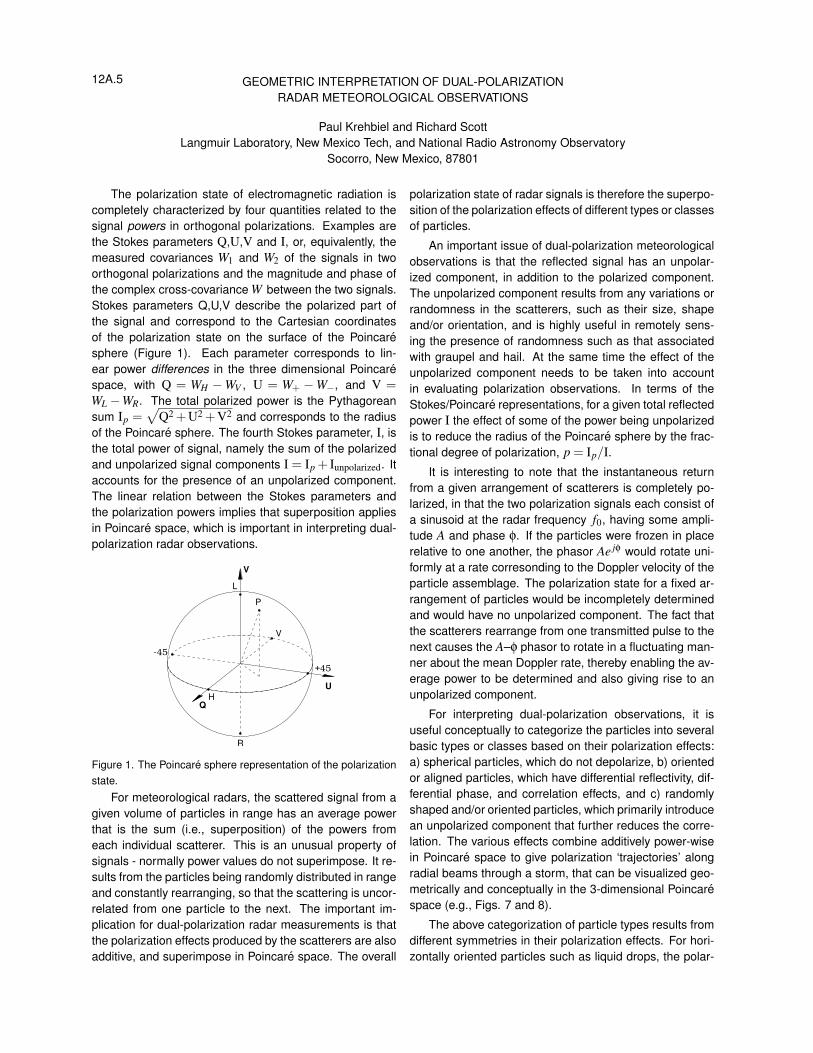
The polarization state of electromagnetic radiation iscompletely characterized by four quantities related to thesignal powers in orthogonal polarizations. Examples arethe Stokes parameters Q,U,V and I, or, equivalently, themeasured covariances W1 and W2 of the signals in twoorthogonal polarizations and the magnitude and phase ofthe complex cross-covariance W between the two signals.Stokes parameters Q,U,V describe the polarized part ofthe signal and correspond to the Cartesian coordinatesof the polarization state on the surface of the Poincaresphere (Figure 1). Each parameter corresponds to lin-ear power differences in the three dimensional Poincarespace, with Q = WH −WV , U = W+ −W−, and V =WL −WR. The total polarized power is the Pythagoreansum Ip =
√Q2 +U2 +V2 and corresponds to the radius
of the Poincare sphere. The fourth Stokes parameter, I, isthe total power of signal, namely the sum of the polarizedand unpolarized signal components I = Ip + Iunpolarized. Itaccounts for the presence of an unpolarized component.The linear relation between the Stokes parameters andthe polarization powers implies that superposition appliesin Poincare space, which is important in interpreting dual-polarization radar observations.
+45
Q
U
V
L
-45
V
H
R
P
Figure 1. The Poincare sphere representation of the polarizationstate.
For meteorological radars, the scattered signal from agiven volume of particles in range has an average powerthat is the sum (i.e., superposition) of the powers fromeach individual scatterer. This is an unusual property ofsignals - normally power values do not superimpose. It re-sults from the particles being randomly distributed in rangeand constantly rearranging, so that the scattering is uncor-related from one particle to the next. The important im-plication for dual-polarization radar measurements is thatthe polarization effects produced by the scatterers are alsoadditive, and superimpose in Poincare space. The overall
polarization state of radar signals is therefore the superpo-sition of the polarization effects of different types or classesof particles.
An important issue of dual-polarization meteorologicalobservations is that the reflected signal has an unpolar-ized component, in addition to the polarized component.The unpolarized component results from any variations orrandomness in the scatterers, such as their size, shapeand/or orientation, and is highly useful in remotely sens-ing the presence of randomness such as that associatedwith graupel and hail. At the same time the effect of theunpolarized component needs to be taken into accountin evaluating polarization observations. In terms of theStokes/Poincare representations, for a given total reflectedpower I the effect of some of the power being unpolarizedis to reduce the radius of the Poincare sphere by the frac-tional degree of polarization, p = Ip/I.
It is interesting to note that the instantaneous returnfrom a given arrangement of scatterers is completely po-larized, in that the two polarization signals each consist ofa sinusoid at the radar frequency f0, having some ampli-tude A and phase φ. If the particles were frozen in placerelative to one another, the phasor Ae jφ would rotate uni-formly at a rate corresonding to the Doppler velocity of theparticle assemblage. The polarization state for a fixed ar-rangement of particles would be incompletely determinedand would have no unpolarized component. The fact thatthe scatterers rearrange from one transmitted pulse to thenext causes the A–φ phasor to rotate in a fluctuating man-ner about the mean Doppler rate, thereby enabling the av-erage power to be determined and also giving rise to anunpolarized component.
For interpreting dual-polarization observations, it isuseful conceptually to categorize the particles into severalbasic types or classes based on their polarization effects:a) spherical particles, which do not depolarize, b) orientedor aligned particles, which have differential reflectivity, dif-ferential phase, and correlation effects, and c) randomlyshaped and/or oriented particles, which primarily introducean unpolarized component that further reduces the corre-lation. The various effects combine additively power-wisein Poincare space to give polarization ‘trajectories’ alongradial beams through a storm, that can be visualized geo-metrically and conceptually in the 3-dimensional Poincarespace (e.g., Figs. 7 and 8).
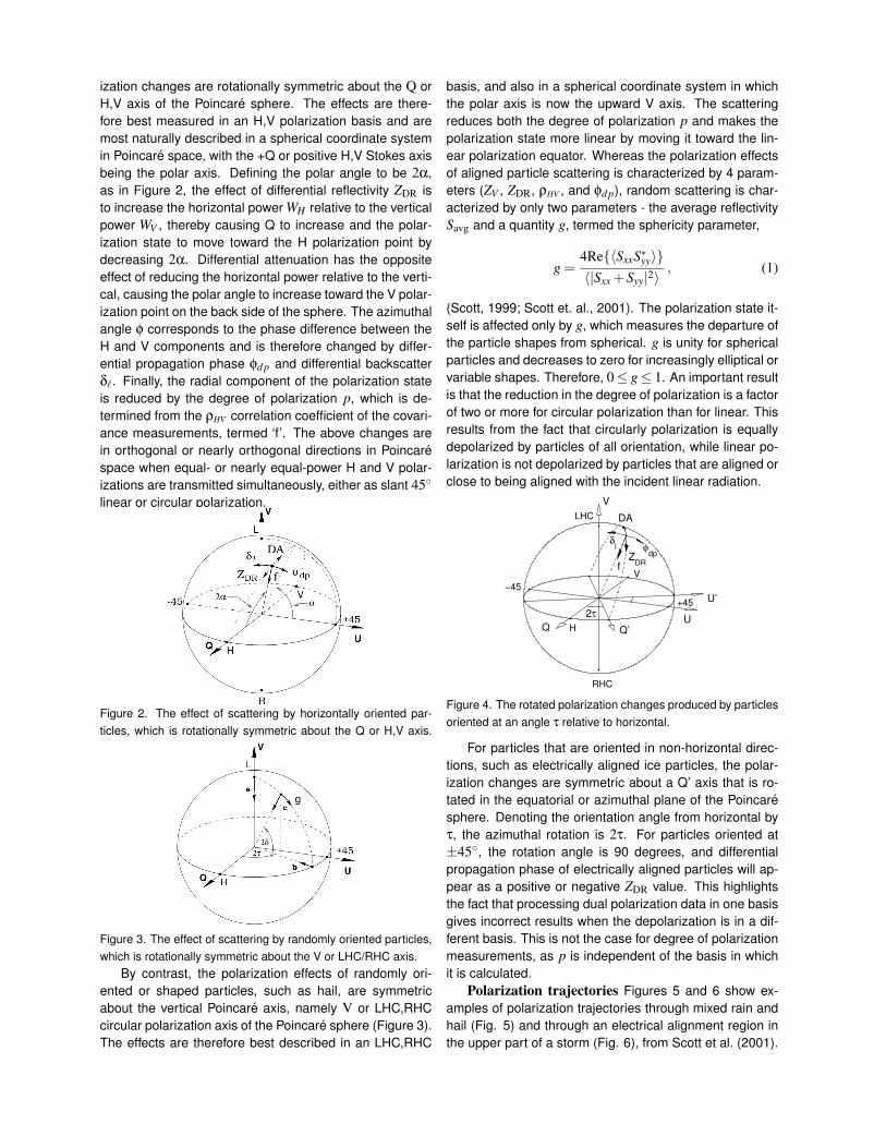
The above categorization of particle types results fromdifferent symmetries in their polarization effects. For hori-zontally oriented particles such as liquid drops, the polar-
ization changes are rotationally symmetric about the Q orH,V axis of the Poincare sphere. The effects are there-fore best measured in an H,V polarization basis and aremost naturally described in a spherical coordinate systemin Poincare space, with the +Q or positive H,V Stokes axisbeing the polar axis. Defining the polar angle to be 2α,as in Figure 2, the effect of differential reflectivity ZDR isto increase the horizontal power WH relative to the verticalpower WV , thereby causing Q to increase and the polar-ization state to move toward the H polarization point bydecreasing 2α. Differential attenuation has the oppositeeffect of reducing the horizontal power relative to the verti-cal, causing the polar angle to increase toward the V polar-ization point on the back side of the sphere. The azimuthalangle φ corresponds to the phase difference between theH and V components and is therefore changed by differ-ential propagation phase φd p and differential backscatterδ`. Finally, the radial component of the polarization stateis reduced by the degree of polarization p, which is de-termined from the ρHV correlation coefficient of the covari-ance measurements, termed ‘f’. The above changes arein orthogonal or nearly orthogonal directions in Poincarespace when equal- or nearly equal-power H and V polar-izations are transmitted simultaneously, either as slant 45◦
linear or circular polarization.
Figure 2. The effect of scattering by horizontally oriented par-ticles, which is rotationally symmetric about the Q or H,V axis.
Figure 3. The effect of scattering by randomly oriented particles,which is rotationally symmetric about the V or LHC/RHC axis.
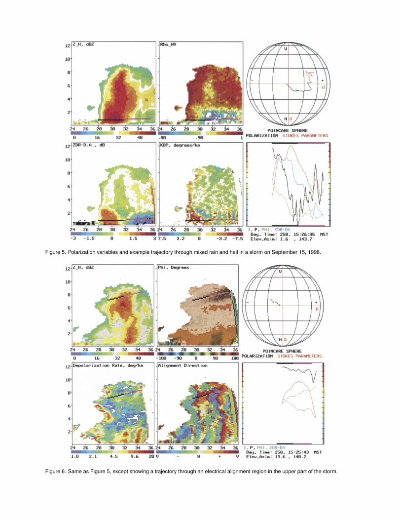
By contrast, the polarization effects of randomly ori-ented or shaped particles, such as hail, are symmetricabout the vertical Poincare axis, namely V or LHC,RHCcircular polarization axis of the Poincare sphere (Figure 3).The effects are therefore best described in an LHC,RHC
basis, and also in a spherical coordinate system in whichthe polar axis is now the upward V axis. The scatteringreduces both the degree of polarization p and makes thepolarization state more linear by moving it toward the lin-ear polarization equator. Whereas the polarization effectsof aligned particle scattering is characterized by 4 param-eters (ZV , ZDR, ρHV , and φd p), random scattering is char-acterized by only two parameters - the average reflectivitySavg and a quantity g, termed the sphericity parameter,
g =4Re{〈SxxS∗yy〉}〈|Sxx +Syy|2〉
, (1)
(Scott, 1999; Scott et. al., 2001). The polarization state it-self is affected only by g, which measures the departure ofthe particle shapes from spherical. g is unity for sphericalparticles and decreases to zero for increasingly elliptical orvariable shapes. Therefore, 0≤ g≤ 1. An important resultis that the reduction in the degree of polarization is a factorof two or more for circular polarization than for linear. Thisresults from the fact that circularly polarization is equallydepolarized by particles of all orientation, while linear po-larization is not depolarized by particles that are aligned orclose to being aligned with the incident linear radiation.
U’
U
+45
φdp
V
ZDR
Q’
DA
f
δl
V
RHC
2τ
LHC
HQ
−45
Figure 4. The rotated polarization changes produced by particlesoriented at an angle τ relative to horizontal.
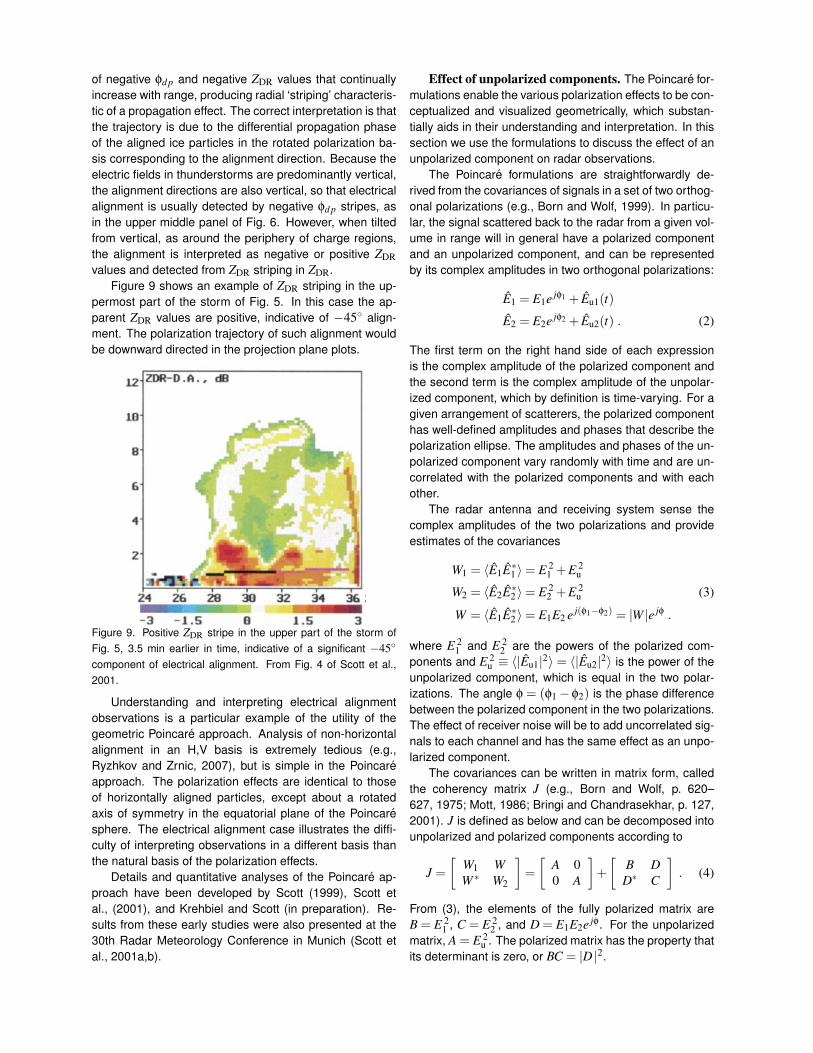
For particles that are oriented in non-horizontal direc-tions, such as electrically aligned ice particles, the polar-ization changes are symmetric about a Q’ axis that is ro-tated in the equatorial or azimuthal plane of the Poincaresphere. Denoting the orientation angle from horizontal byτ, the azimuthal rotation is 2τ. For particles oriented at±45◦, the rotation angle is 90 degrees, and differentialpropagation phase of electrically aligned particles will ap-pear as a positive or negative ZDR value. This highlightsthe fact that processing dual polarization data in one basisgives incorrect results when the depolarization is in a dif-ferent basis. This is not the case for degree of polarizationmeasurements, as p is independent of the basis in whichit is calculated.
Polarization trajectories Figures 5 and 6 show ex-amples of polarization trajectories through mixed rain andhail (Fig. 5) and through an electrical alignment region inthe upper part of a storm (Fig. 6), from Scott et al. (2001).
Figure 5. Polarization variables and example trajectory through mixed rain and hail in a storm on September 15, 1998.
Figure 6. Same as Figure 5, except showing a trajectory through an electrical alignment region in the upper part of the storm.
APRIL 2001 637S C O T T E T A L .
FIG. 5. Same as Fig. 4 but another 3 min later in the storm, at 1526:35. The negative apparent ZDR values below 2-km altitude on theright side of the storm indicate that significant differential attenuation occurred in passing through the main precipitation region. Note thesustained decrease in �HV in the same part of the storm, indicating that the radar signal developed an unpolarized component in propagatingthrough the main precipitation region, which by now undoubtedly consisted of mixed hail and rain.
that the negative ZDR region did not extend down to theground does not mean that the hail had completely melt-ed in the lower altitudes. Rather, any negative ZDR ofthe hail would tend to have been offset by positive ZDRfrom liquid drops. The apparent ZDR values were ap-proximately zero in the lower part of the hailshaft, most-ly as a result of differential attenuation but possibly alsodue to the above cancellation effect. As before, invertedpolarity Kdp values existed on the far side of the meltinghail, indicating that the hail produced positive �� uponbackscatter, consistent with vertical elongation.From the above, the precipitation in the lower part
of the storm was almost certainly mixed phase. Thisundoubtedly contributed to the large observed reductionin the correlation coefficient. Over large regions �HVwasbelow 0.8, and within these regions decreased to as lowas 0.70. Of particular significance is the result that thecorrelation remained low on the far side of the storm.Such ‘‘shadowing’’ is good evidence of a propagationeffect; in this case the radar signal developed a sub-
stantial unpolarized component while propagatingthrough the low-�HV precipitation core, and accumulatedto the level shown. Like � dp, the development of anunpolarized component would be the result of forwardscattering, in this case by mixed-phase precipitationhaving a variety of shapes and orientations, and wouldbe cumulative with range.
d. Signal processing
The above observations were obtained with an in-expensive PC-based digital signal processor (Rison etal. 1993). The processor was originally developed forthe Convection and Precipitation/Electrification pro-gram in 1991 and used to study the electrical alignmentof ice crystals (Chen 1994; Krehbiel et al. 1996). TwoMotorola 56001 digital signal processors averaged thesignals from 32 transmitted pulses (16 ms at a 2-kHzpulse repetition frequency), at each of 250 1-�s rangegates (37.5-km range). One digital signal processor
Zdr
φdp
φdp δl
DA
DA
Q
U
+45−45
H
V
LHC
Figure 7. Top: Expanded view of the polarization trajectory ofFig. 5. Bottom: Conceptual illustration of how the polarizationstate at a given range gate is arrived at from the cumulative prop-agation effects of differential attenuation (DA) and phase (φd p)(red), and the backscatter effects of differential phase (δ`) andreflectivity ZDR (blue).
The trajectories are shown as viewed from above thePoincare sphere and show how the Stokes parameters Qand U change with range. In both figures the trajectoriesbegin near the circular polarization point in the center ofthe projection, corresponding to LHC transmitted polar-ization. An expanded view of the trajectory for the mixedrain/hail observation is shown in Figure 7. The trajectoryinitially developed downward and to the right as a resultof the combined effects of ZDR and φd p upon entering therain region, then to the right as a result of steadly increas-ing φd p. The effects of ZDR and differential attenuationappear to remain constant during the latter range interval.Upon leaving the strong rain region, φd p stops increasingand ZDR gradually decreases, moving the trajectory up-ward toward the V polarization point and revealing the cu-mulative effect of differential attenuation.
The bottom panel of Figure 7 illustrates conceptuallyhow the polarization state at a given range gate is reached.The red vectors show the cumulative propagation effectsof differential attenuation and phase, both before and afterbackscatter, while the blue vector shows the effect of
APRIL 2001 639S C O T T E T A L .
FIG. 7. RHI scan at 1525:43, showing vertical electrical alignment in the upper part of the storm. The alignment is indicated by the darkradial band in the � panel (upper middle) and by the the red-blue region in the alignment direction panel (lower middle).
FIG. 8. Alignment direction vectors at three ranges from the radar, reconstructed from a 3D volume scan of the storm between 1524:07and 1527:18. The observations are on surfaces of constant range from the radar and show the storm as it would be viewed from the radar.Vertical or near-vertical alignment is indicated by the black vectors and shows that strong electrification existed in the upper-left part of thestorm, and in the middle-upper part of the main precipitation shaft (see text). The altitudes are in km MSL.
638 VOLUME 18J O U R N A L O F A T M O S P H E R I C A N D O C E A N I C T E C H N O L O G Y
FIG. 6. The polarization changes produced by nonhorizontallyaligned particles. The dotted lines indicate the polarization changesproduced by horizontally oriented particles; the solid lines show thechanges due to particles oriented at an angle � relative to horizontal.
(DSP) processed the digitized outputs of matched log-arithmic intermediate frequency amplifiers in each re-ceiver channel to obtain WH and WV. The other DSPcorrelated the outputs of coherent, constant-phase am-plitude limiters in the two receiver channels to obtainthe magnitude and phase of . The 32-pulse averaged�HVdata were read into the CPU and stored on disk forpostprocessing. To reduce the size of the data files, suc-cessive pairs of 32-pulse data were averaged before writ-ing to disk. At the same time the data were processedto produce a real-time display. The results shown in thispaper are from postprocessing, but essentially the samesoftware was used to generate the real-time display. Theprocessing further smoothed the data using a running3-gate (450 m) range average and a 3-ray or angularrunning average. Since each data ray consisted of theaverage of (32 � 2) transmitted pulses to begin with,a total of 9 � 64 � 576 samples were averaged. Anadditional 3-gate running range average was used tosmooth the range-differentiated Kdp values.
4. Determining particle alignment directionsNonhorizontal alignment occurs as a result of elec-
trical forces, which orient populations of ice crystals inthe direction of the local electric field (Hendry and Mc-Cormick 1976; Chen 1994; Metcalf 1995, 1997; Kreh-biel et al. 1996). The alignment is detected by the effectthat the aligned crystals have on propagation of the radarsignal. In particular, the crystals cause cumulative dif-ferential propagation phase shift � dp between the com-ponents parallel and perpendicular to the alignment di-rection. Attenuation and differential attenuation can beneglected, even at 3-cm wavelength, because the par-ticles are ice-form. Backscatter effects (ZDR and/or ��)from the aligned particles also appear not to be impor-tant. Rather, the aligned ice crystals appear to be smalland the backscattered signal tends to be dominated bylarger hydrometeors (graupel or hail) that serve as a‘‘detector’’ of the differential phase produced by thealigned crystals (McCormick and Hendry 1979; Hendryand Antar 1982; Krehbiel et al. 1996).5Particles aligned at an angle � relative to the hori-
zontal depolarize the radar signal in the same manneras horizontal particles, except about an axis of symmetrycorresponding to the alignment direction. As discussedin the appendix, the direction of � dp and ZDR changesare rotated by an angle 2� about the vertical axis of thePoincare sphere.6 Figure 6 illustrates the effect of this
5 Metcalf (1997) has disputed the point that backscatter effects arenot important; full resolution of this question would be obtained byalternately transmitting left- and right-circular polarizations, as dis-cussed later.
6 The rotation effect was shown in a series of papers by Barge(1972), McCormick et al. (1972), Humphries (1974), McCormick andHendry (1975), McCormick and Hendry (1979), and McCormick(1979) using a planar representation of the polarization state.
on the Poincare sphere projection view of the earlierfigures. For vertical orientation, � dp and ZDR would bein the opposite direction from that for horizontal ori-entation, causing the measured values of � dp and ZDR(dB) to be negative. For particles oriented at � � �45�,� dp changes would be upward and would be interpretedas negative ZDR values, while positive ZDR would be tothe right and interpreted as a � dp effect.When the depolarization is dominated by differential
propagation phase (� dp), the alignment direction is read-ily determined from the change in the polarization statebetween successive range gates. Graphically, a line con-structed perpendicular to the � dp change in Fig. 6 (i.e.,in the ZDR direction), will be oriented at an angle 2�relative to the H axis. Computationally, the alignmentdirections are determined by transforming the covari-ance measurements into the Stokes parameters and usingthe changes in Q and U to obtain � (Scott 1999).Electrical alignment is often vertical or nearly vertical
and is observed in the upper and middle part of storms.The electrical nature of the alignment is clearly dem-onstrated by sudden decreases in the alignment signatureat the time of lightning. Vertical orientation comes aboutonly as a result of electrical alignment and is a goodindicator of electrification. The result that electric align-ment is predominantly vertical agrees well with in situmeasurements of the electric field inside storms (e.g.,Stolzenburg et al. 1998a,b).
a. ObservationsFigures 7 and 8 show examples of electrical alignment
from the 15 September storm. The Fig. 7 data are from
Figure 8. Top: Expanded view of the polarization trajectoryof Fig. 6. Bottom: Illustration of how non-horizontal alignmentchanges the directions of φd p and ZDR effects. Normal H,V pro-cessing interprets the changes as if they were produced by hori-zontally oriented particles (dotted arrows), and misinterprets thechange as being due to negative ZDR and negative φd p values.
differential phase upon backscatter and differential reflec-tivity. A side view from in front of the Poincare spherewould show how the degree of polarization changes dueto variability in particle shapes and random particle ori-entations. Both views would show the polarization obser-vations in Cartesian coordinates, for which superpositionholds. The trajectory of Fig. 7 is thus the superpositionof those for the horizontally oriented rain and randomlyshaped and oriented hail. Because of this it should bepossible in principle to decompose the two contributionswith appropriate polarization-diverse measurements.
The polarization trajectory for the electrical alignmentobservations (Figure 8) exhibits a different behavior, de-veloping upward and to the left with increasing range, thatis sustained until the radar beam exited the storm. For theexpected case in which the depolarization by aligned icecrystals is due primarily to φd p and not to ZDR effects, theorientation of the trajectory is indicative of the alignmentdirection, as in the bottom part of Fig. 8. However, theH,V processing interprets the trajectory as a combination
of negative φd p and negative ZDR values that continuallyincrease with range, producing radial ‘striping’ characteris-tic of a propagation effect. The correct interpretation is thatthe trajectory is due to the differential propagation phaseof the aligned ice particles in the rotated polarization ba-sis corresponding to the alignment direction. Because theelectric fields in thunderstorms are predominantly vertical,the alignment directions are also vertical, so that electricalalignment is usually detected by negative φd p stripes, asin the upper middle panel of Fig. 6. However, when tiltedfrom vertical, as around the periphery of charge regions,the alignment is interpreted as negative or positive ZDRvalues and detected from ZDR striping in ZDR.
Figure 9 shows an example of ZDR striping in the up-permost part of the storm of Fig. 5. In this case the ap-parent ZDR values are positive, indicative of −45◦ align-ment. The polarization trajectory of such alignment wouldbe downward directed in the projection plane plots.
636 VOLUME 18J O U R N A L O F A T M O S P H E R I C A N D O C E A N I C T E C H N O L O G Y
FIG. 4. Vertical cross section at the same azimuth as Fig. 2 but 3 min later, at 1523:05, and showing the polarization trajectory. Note theincreased positive ZDR values in the inflow region on the left, the lower altitude at which liquid drops start to appear in the hailshaft, andthe enhanced negative ZDR values where the hail would be expected to be melting. The latter region was associated with reductions of �HV
below 0.80.
the storm exhibited features similar to those of Fig. 3.One difference is that, upon entering the storm, the po-larization state changed along a 45� path downward andto the right. This is typical of entering a rain region andreflects the combined effects of increasing ZDR and � dp,whose changes are comparable at 3-cm wavelength onthe Poincare sphere. The upward meandering of the po-larization state during the final part of the trajectory isdue to the decrease in ZDR on the far side of the storm.At the final gate the H and V powers had returned tonearly equal values, indicating that differential attenu-ation was not significant.An additional feature of interest in the Fig. 4 obser-
vations is the faint ray of slightly positive ZDR valuesin the upper part of the storm. This is not an artifact ofantenna sidelobes but indicates the presence of electri-cally aligned ice crystals. Electrical alignment is dis-cussed later; the ZDR artifact occurs because the ice crys-tals were oriented at an intermediate angle between hor-izontal and vertical, which caused the the polarization
state to move downward in the projection view, in thesame direction as ZDR from liquid drops.The radar scan at 1526:35 (Fig. 5) showed continued
descent and intensification of the precipitation at lowlevels, and a further decrease in �HV below 2-km altitude.Positive ZDR values were no longer seen between thehailshaft and ground, but liquid drops continued to bepresent throughout much or all of the main precipitationregion. This is inferred from the fact that the apparentZDR values on the far side of the storm were stronglynegative (�3 dB), indicating that a significant amountof differential attenuation had occurred in passingthrough the precipitation. The effect of the differentialattenuation is seen in the polarization trajectory, whichdeveloped well above the equal-power line along thefinal part of the range cursor, indicating that the powerin H had become substantially less than in V.The lower part of the hailshaft continued to exhibit
negative ZDR values of about �1 dB, by now over alarger, somewhat shallower horizontal region. The fact
Figure 9. Positive ZDR stripe in the upper part of the storm ofFig. 5, 3.5 min earlier in time, indicative of a significant −45◦
component of electrical alignment. From Fig. 4 of Scott et al.,2001.
Understanding and interpreting electrical alignmentobservations is a particular example of the utility of thegeometric Poincare approach. Analysis of non-horizontalalignment in an H,V basis is extremely tedious (e.g.,Ryzhkov and Zrnic, 2007), but is simple in the Poincareapproach. The polarization effects are identical to thoseof horizontally aligned particles, except about a rotatedaxis of symmetry in the equatorial plane of the Poincaresphere. The electrical alignment case illustrates the diffi-culty of interpreting observations in a different basis thanthe natural basis of the polarization effects.
Details and quantitative analyses of the Poincare ap-proach have been developed by Scott (1999), Scott etal., (2001), and Krehbiel and Scott (in preparation). Re-sults from these early studies were also presented at the30th Radar Meteorology Conference in Munich (Scott etal., 2001a,b).
Effect of unpolarized components. The Poincare for-mulations enable the various polarization effects to be con-ceptualized and visualized geometrically, which substan-tially aids in their understanding and interpretation. In thissection we use the formulations to discuss the effect of anunpolarized component on radar observations.
The Poincare formulations are straightforwardly de-rived from the covariances of signals in a set of two orthog-onal polarizations (e.g., Born and Wolf, 1999). In particu-lar, the signal scattered back to the radar from a given vol-ume in range will in general have a polarized componentand an unpolarized component, and can be representedby its complex amplitudes in two orthogonal polarizations:
E1 = E1e jφ1 + Eu1(t)
E2 = E2e jφ2 + Eu2(t) . (2)
The first term on the right hand side of each expressionis the complex amplitude of the polarized component andthe second term is the complex amplitude of the unpolar-ized component, which by definition is time-varying. For agiven arrangement of scatterers, the polarized componenthas well-defined amplitudes and phases that describe thepolarization ellipse. The amplitudes and phases of the un-polarized component vary randomly with time and are un-correlated with the polarized components and with eachother.
The radar antenna and receiving system sense thecomplex amplitudes of the two polarizations and provideestimates of the covariances
W1 = 〈E1E∗1 〉= E 21 +E 2
u
W2 = 〈E2E∗2 〉= E 22 +E 2
u (3)
W = 〈E1E∗2 〉= E1E2 e j(φ1−φ2) = |W |e jφ .
where E 21 and E 2
2 are the powers of the polarized com-ponents and E 2
u ≡ 〈|Eu1|2〉 = 〈|Eu2|2〉 is the power of theunpolarized component, which is equal in the two polar-izations. The angle φ = (φ1−φ2) is the phase differencebetween the polarized component in the two polarizations.The effect of receiver noise will be to add uncorrelated sig-nals to each channel and has the same effect as an unpo-larized component.
The covariances can be written in matrix form, calledthe coherency matrix J (e.g., Born and Wolf, p. 620–627, 1975; Mott, 1986; Bringi and Chandrasekhar, p. 127,2001). J is defined as below and can be decomposed intounpolarized and polarized components according to
J =
[W1 WW ∗ W2
]=
[A 00 A
]+
[B D
D∗ C
]. (4)
From (3), the elements of the fully polarized matrix areB = E 2
1 , C = E 22 , and D = E1E2e jφ. For the unpolarized
matrix, A = E 2u . The polarized matrix has the property that
its determinant is zero, or BC = |D |2.
The covariances determine four quantities: W1, W2,and |W | and 6 W = φ (or, equivalently, Re[W] and Im[W]).The decomposed covariance matrices (4) are describedby five quantities (A, B, C, |D|, and 6 D), whose valuescan be obtained from the covariances and from the polar-ization constraint BC = |D |2. In particular,
2A = (W1 +W2)−√(W1−W2)2 +4|W |2)
2B = (W1−W2)+√(W1−W2)2 +4|W |2)
2C = (W2−W1)+√(W1−W2)2 +4|W |2)
D =W . (5)
The decomposed quantities involve only the sum and dif-ference of W1 and W2 and not W1 or W2 individually. Fur-thermore, the polarized quantities B and C involve only thedifference term, (W1−W2). The result that D =W is seenby inspection of (4) and follows from the fact that the cross-covariance W is unaffected by the presence of an unpolar-ized component (or by receiver noise).
The above quantities have the interpretation that(W1 +W2) is the total signal power I, (B+C) is the to-tal polarized power Ip, and 2A is the total unpolarizedpower, which is equally split between the two polarizations.(W1 −W2) is the difference of the orthogonal powers inthe measurement basis and corresponds to the Stokes pa-rameter in that basis. From (5), the total polarized power(B+C) is given by
B+C =√
(W1−W2)2 +4|W |2 = Ip . (6)
This expresses the polarized power in terms of the powerdifference (W1−W2) and is a fundamental result for deriv-ing the Poincare and Stokes results. In particular, since
W = |W |e jφ = |W |cosφ+ j |W |sinφ (7)
one has that 4|W |2 = (2|W |cosφ)2 +(2|W |sinφ)2. Thus,the expression for the polarized power becomes
B+C =√(W1−W2)2 +(2|W |cosφ)2 +(2|W |sinφ)2
≡ Ip . (8)
The total polarized power is therefore the sum of three or-thogonal quantities: (W1−W2), 2|W |cosφ, and 2|W |sinφ.The Pythagorean nature of this result is readily apparentand can be illustrated graphically. As noted earlier, the(W1−W2) axis corresponds to the Stokes parameter in themeasurement basis. For the case in which the measure-ments are in an H–V basis, W1−W2 = WH −WV , whichis the Stokes parameter Q. Similarly, the cross-covarianceW becomes WHV.
Considering (WH −WV ) to be the ‘z’ axis of a right-handed 3-dimensional coordinate system, it can be shown
that the x and y axes (i.e., 2|WHV |cosφ and 2|WHV |sinφ)correspond to
Returning to the decomposition matrices, and consid-ering the two polarizations to be H and V, (5) become
2A = I− Ip = I(1− p)
2B = Ip +Q2C = Ip−Q (10)
Considering ZDR first, its value is usually determined fromthe ratio WH/WV . However, from (4), this corresponds to
ZDR =WH
WV=
B+AC+A
=I+QI−Q
. (11)
This gives the correct result for ZDR when the unpolarizedpower A is zero or negligibly small, but an increasinglybiased result when an unpolarized component is present.This is because A is the same in both polarizations, whileB and C are different in situations of interest. The correctformulation for differential reflectivity is the ratio of B and Cby themselves, namely the ratio of the polarized powers.From (10), we have that
ZDR =BC
=Ip +QIp−Q
=1+Q/Ip
1−Q/Ip. (12)
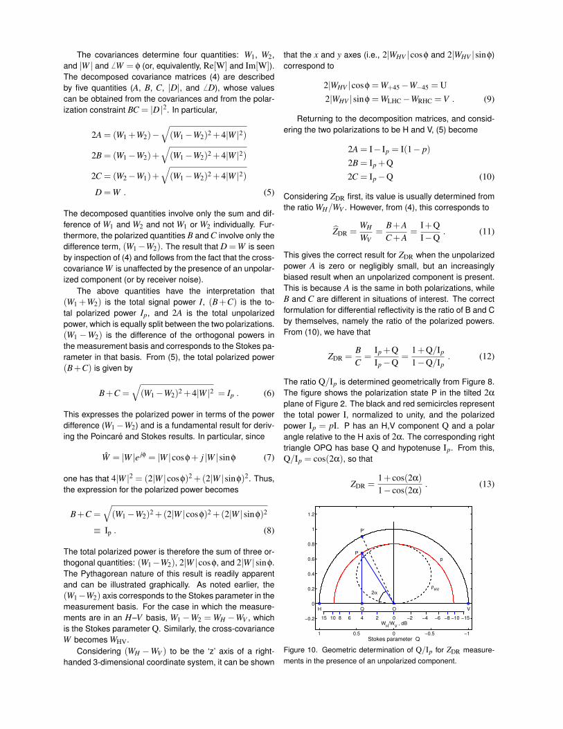
The ratio Q/Ip is determined geometrically from Figure 8.The figure shows the polarization state P in the tilted 2α
plane of Figure 2. The black and red semicircles representthe total power I, normalized to unity, and the polarizedpower Ip = pI. P has an H,V component Q and a polarangle relative to the H axis of 2α. The corresponding righttriangle OPQ has base Q and hypotenuse Ip. From this,Q/Ip = cos(2α), so that
ZDR =1+ cos(2α)
1− cos(2α). (13)
1 0.5 0 −0.5 −1
−0.2
0
0.2
0.4
0.6
0.8
1
1.2
2α
Stokes parameter Q
P
P’
Q O
ρHV
p
H V
024681015 −2 −4 −6 −8 −10 −15W
H/W
V , dB
Figure 10. Geometric determination of Q/Ip for ZDR measure-ments in the presence of an unpolarized component.
−1 −0.5 0 0.5 1−10
−8
−6
−4
−2
0
2
4
6
8
10
Stokes parameter Q
Zdr,
dB
Error in ZDR
Determination, p = 0.8
Correct ZDR
WH
/WV , biased
ρHV
x 10
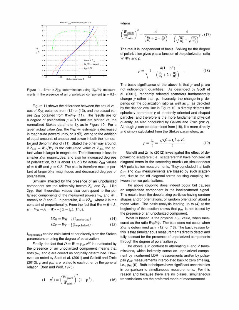
Figure 11. Error in ZDR determination using WH /WV measure-ments in the presence of an unpolarized component (p = 0.8).
Figure 11 shows the difference between the actual val-ues of ZDR obtained from (12) or (13), and the biased val-ues ZDR obtained from WH /WV (11). The results are fora degree of polarization p = 0.8 and are plotted vs. thenormalized Stokes parameter Q, as in Figure 10. For agiven actual value ZDR, the WH /WV estimate is decreasedin magnitude (toward unity, or 0 dB), owing to the additionof equal amounts of unpolarized power in both the numera-tor and denominator of (11). Stated the other way around,if ZDR = WH/WV is the calculated value of ZDR, the ac-tual value is larger in magnitude. The difference is less forsmaller ZDR magnitudes, and also for increased degreesof polarization, but is about 1.5 dB for actual ZDR valuesof ' 6 dB and p = 0.8. The bias is therefore most impor-tant at larger ZDR magnitudes and decreased degrees ofpolarization.
Similarly affected by the presence of an unpolarizedcomponent are the reflectivity factors ZH and ZV . LikeZDR, their theoretical values also correspond to the po-larized components of the measured powers WH and WV ,namely to B and C. In particular, B = kZH , where k is theconstant of proportionality. From the fact that WH = B+A,B =WH −A =WH − 1
2 (I− Ip). Thus,
kZH =WH − 12 (Iunpolarized) (14)
kZV =WV − 12 (Iunpolarized) . (15)
Iunpolarized can be calculated either directly from the Stokesparameters or using the degree of polarization.
Finally, the fact that D = W = ρHV e jφ is unaffected bythe presence of an unpolarized component means thatboth ρHV and φ are correct as originally determined. How-ever, as noted by Scott et al. (2001) and Galletti and Zrnic(2012), p and ρHV are related to each other by the generalrelation (Born and Wolf, 1975)
(1− p2) =
(W geom
W arith
)2
(1−ρ2) , (16)
where(W geom
W arith
)2
=4(
W1W2
+2+ W2W1
) =4(√
W1W2
+√
W2W1
)2 . (17)
The result is independent of basis. Solving for the degreeof polarization gives p as a function of the polarization ratioW1/W2 and ρ:
p =
√√√√1− 4(1−ρ2)(W1W2
+2+ W2W1
) . (18)
The basic significance of the above is that p and ρ arenot independent quantities. As described by Scott etal. (2001), randomly oriented scatterers fundamentallychange p rather than ρ. Inversely, the change in ρ de-pends on the polarization ratio as well as p, as depictedby the dashed oval line in Figure 10. p directly detects thesphericity parameter g of randomly oriented and shapedparticles, and therefore is the more fundamental physicalquantity, as also concluded by Galletti and Zrnic (2012).Although p can be determined from (18), it is more directlyand simply calculated from the Stokes parameters, as
p =Ip
I=
√Q2 +U2 +V2
I. (19)
Galletti and Zrnic (2012) investigated the effect of de-polarizing scatterers (i.e., scatterers that have non-zero offdiagonal terms in the scattering matrix) on simultaneousH,V polarization measurements. They concluded that bothρHV and ZDR measurements are biased by such scatter-ers, due to the off diagonal terms causing coupling be-tween the two polarizations.
The above coupling does indeed occur but causesan unpolarized component in the backscattered signal.This results from the depolarizing particles having randomshapes and/or orientations, or random orientation about amean value. The basic analysis leading up to (4) at thebeginning of this section shows that ρHV is not biased bythe presence of an unpolarized component.
What is biased is the physical ZDR value, when mea-sured as the ratio WH /WV . The bias does not occur whenZDR is determined as in (12) or (13). The basic reason forthis is that simultaneous measurements directly detect andfully account for the presence of unpolarized componentsthrough the degree of polarization p.
The above is in contrast to alternating H and V trans-missions, which indirectly sense an unpolarized compo-nent by incoherent LDR measurements and/or by pulse-pair ρHV measurements interpolated back to zero time lag,i.e., ρHV (0). Both techniques have significant uncertaintiesin comparison to simultaneous measurements. For thisreason and because there are no biases, simultaneoustransmissions are the preferred mode of measurement.
Summary. The correct procedure for analyzing dual-polarization observations in an H,V basis is first to calcu-late the Stokes parameters from the covariance measure-ments, according to
I =WH +WV
Q =WH −WV
U = 2|WHV |cosφHV
V = 2|WHV |sinφHV . (20)
Then calculate the polarized power Ip and degree of po-larization p from
Ip =√
Q2 +U2 +V2 (21)p = Ip/I . (22)
Calculate the H,V precipitation parameters ZH , ZV andZDR from
kZH =WH − 12 (I− Ip) (23)
kZV =WV − 12 (I− Ip) , (24)
ZDR =Ip +QIp−Q
, (25)
and ρHV and φ from
ρHV = |WHV | (26)φ = φHV . (27)
Finally, display the precipitation variables of interest, in-cluding p and Ip, along with top (−Q vs. U), front (V vs.U), and side (V vs. −Q) projection views of the polariza-tion trajectory along the current or selected radial beam ofthe radar (or a 3-D rotatable view of unit Poincare sphereand trajectory).
REFERENCES
V. N. Bringi and V. Chandrasekhar, Polarimetric DopplerWeather Radar. Principles and Applications. Cambridge,U.K.: Cambridge Univ. Press, 2001.
M. Born and E. Wolf, Principles of Optics: Electromag-netic Theory of Propagation, Interference and Diffractionof Light, 7th ed., Cambridge Univ. Press, 1999.
Galletti, M. and D. S. Zrnic, Degree of polarization at si-multaneous transmit: Theoretical aspects, IEEE Geosci.and Remote Sensing Letts., 9, 383-387, May 2012.
Krehbiel, P., and R. Scott, A geometric approach tocharacterizing and interpreting dual-polarization radar me-teorological observations, working document, 1999,2005.
Mott, H., Polarization in Antennas and Radar, J. Wiley,New York, 1986.
Ryzhkov, A., and D. S. Zrnic, Depolarization in ice crys-tals and its effect on radar polarimetric measurements, J.Atmos. Oceanic Technol., 24, 1256-1267, 2007.
Scott, R., Dual-polarization radar meteorology: A ge-ometrical approach, Ph.D. Diss., New Mexico Instituteof Mining and Technology, 129 pp., 1999 (available athttp://lightning.nmt.edu/radar).
Scott, R., P. Krehbiel, and W. Rison, The use of si-multaneous horizontal and vertical transmissions for dual-polarization radar meteorological observations, J. Atmos.and Oceanic Tech., 18, 629-648, 2001.
Scott, R., and P. Krehbiel, A geometric approachto characterizing and interpreting dual-polarizationradar meteorological observations, paper 5B.1, 30thConf./ Radar Meteorol., Munich, 2001 (available athttp://lightning.nmt.edu/radar).
Scott, R., P. Krehbiel, and W. Rison, The use ofsimultaneous horizontal and vertical transmissions fordual-polarization radar meteorological observations, paper5B.2, 30th Conf./ Radar Meteorol., Munich, 2001 (availableat http://lightning.nmt.edu/radar).