13 OCTOBER 2020 The Mathematics of Musical Composition Professor Sarah Hart Introduction Pattern and structure are essential to music. This lecture will explore the mathematics of musical composition, from musical symmetries like transcription or inversion, that have been in use for centuries, to more recent experimentation with the use of mathematical forms such as fractal sequences to produce intriguing effects. Music involves pitch, melody, and rhythm. The earliest music, before instruments were made that could make specific sounds, must have been made largely with rhythm: clapping, stamping, or repetitive vocalisations. Before we are even born, after all, we are surrounded by the iambic pentameters of our own mothers’ heartbeats. Percussion instruments like drums, gongs, bells, exist in various forms in almost every culture. Later, along with our own voices, instruments were invented that could play defined pitches. Melody and harmony were developed. Music started to acquire forms, and to be written down. These forms developed along different lines in different cultures. Today’s lecture focuses on the Western Classical tradition because that has been the basis of my own musical experience. There are fascinating stories to tell about the mathematics connected to other musical traditions, but I am not the person to tell them. I have given some suggestions (references [1] – [5]) for books on music beyond the Western classical canon at the end of these notes, as a starting point for further exploration if you are interested. We begin by gathering together the few pieces of musical notation that we will need. A primer on musical notation In Western tradition, the smallest difference in pitch between two notes is a semitone. Two notes an octave apart have twelve semitones between them. Notes one or more octaves apart are given the same name; we say they are in the same ‘pitch class’. The note names are shown on the diagram of the piano keyboard below. Note names on a piano keyboard The black note between F and G, for example, is a semitone higher, or ‘sharper’ than F, but also a semitone lower, or ‘flatter’ than G. So, we can call it F ♯ or G ♭ . The choice is essentially arbitrary, but there are various conventions which we won’t go into here. The octave can also be divided into scales – the diatonic scale has seven distinct pitches. For instance, the diatonic scale of C major consists of the white notes C, D, E, F, G, A, B and finally C. We can play the same major scale starting in any key, by repeating the exact sequence of gaps between the notes: tone, tone, semitone, tone, tone, tone, semitone. Starting from G, for example, the major scale goes G, A, B, C, D, E, F ♯ , G. A piece in the ‘key of G major’ would tend to end on G, and the notes that make up the music would tend to be drawn mostly, if not entirely, from the notes in the G major scale. (See Lecture 2 in this series for a lot
Transcript
13 OCTOBER 2020
The Mathematics of Musical Composition
Professor Sarah Hart
Introduction Pattern and structure are essential to music. This lecture will explore the mathematics of musical composition, from musical symmetries like transcription or inversion, that have been in use for centuries, to more recent experimentation with the use of mathematical forms such as fractal sequences to produce intriguing effects. Music involves pitch, melody, and rhythm. The earliest music, before instruments were made that could make specific sounds, must have been made largely with rhythm: clapping, stamping, or repetitive vocalisations. Before we are even born, after all, we are surrounded by the iambic pentameters of our own mothers’ heartbeats. Percussion instruments like drums, gongs, bells, exist in various forms in almost every culture. Later, along with our own voices, instruments were invented that could play defined pitches. Melody and harmony were developed. Music started to acquire forms, and to be written down. These forms developed along different lines in different cultures. Today’s lecture focuses on the Western Classical tradition because that has been the basis of my own musical experience. There are fascinating stories to tell about the mathematics connected to other musical traditions, but I am not the person to tell them. I have given some suggestions (references [1] – [5]) for books on music beyond the Western classical canon at the end of these notes, as a starting point for further exploration if you are interested. We begin by gathering together the few pieces of musical notation that we will need.
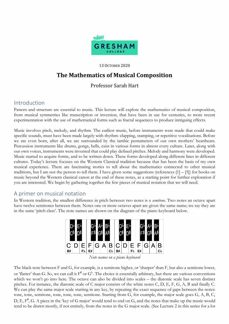
A primer on musical notation In Western tradition, the smallest difference in pitch between two notes is a semitone. Two notes an octave apart have twelve semitones between them. Notes one or more octaves apart are given the same name; we say they are in the same ‘pitch class’. The note names are shown on the diagram of the piano keyboard below.
Note names on a piano keyboard
The black note between F and G, for example, is a semitone higher, or ‘sharper’ than F, but also a semitone lower,
or ‘flatter’ than G. So, we can call it F♯ or G♭. The choice is essentially arbitrary, but there are various conventions which we won’t go into here. The octave can also be divided into scales – the diatonic scale has seven distinct pitches. For instance, the diatonic scale of C major consists of the white notes C, D, E, F, G, A, B and finally C. We can play the same major scale starting in any key, by repeating the exact sequence of gaps between the notes: tone, tone, semitone, tone, tone, tone, semitone. Starting from G, for example, the major scale goes G, A, B, C,
D, E, F♯, G. A piece in the ‘key of G major’ would tend to end on G, and the notes that make up the music would tend to be drawn mostly, if not entirely, from the notes in the G major scale. (See Lecture 2 in this series for a lot
2
more detail on notes, tuning and scales.) There are also minor scales, and pentatonic scales, but we will not concern ourselves with them here. Some of the musical symmetries we will encounter relate to the way music is written as notes on a stave. Music was being routinely written down in the West by the Middle Ages. Guido D’Arezzo, an Italian monk, is usually credited with the invention of the stave notation, in the early eleventh century, to help choristers learn tunes they had never heard before. There had been earlier attempts to write down music, using symbols called neumes. These were written above the words to be sung. An upwards curve meant that your voice should rise in pitch on that syllable, for example. But you were not told by how much, so these were likely only ever meant to be aides-memoires. Guido D’Arezzo put the neumes on staves which indicated particular notes. (His staves only had four lines, not our modern five.) Then, gradually, ‘mensural’ notation developed, where you were told not only what pitch to play or sing, but how long the note should last. It took another couple of centuries before things like bar lines were commonplace, but when we look at music from the 16th and 17th centuries and beyond, it is recognisably
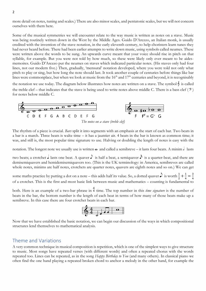
the notation we use today. The diagram below illustrates how notes are written on a stave. The symbol G is called
the treble clef – that indicates that the stave is being used to write notes above middle C. There is a bass clef ( ? ) for notes below middle C.
The notes on a stave (treble clef)
The rhythm of a piece is crucial. Bars split it into segments with an emphasis at the start of each bar. Two beats in a bar is a march. Three beats is waltz time – it has a jauntier air. 4 beats in the bar is known as common time; it was, and still is, the most popular time signature to use. Halving or doubling the length of notes is easy with the
notation. The longest note we usually use is written w and called a semibreve – it lasts four beats. A minim h lasts
two beats; a crotchet qlasts one beat. A quaver e is half a beat, a semiquaver s is a quarter-beat, and there are
demisemiquavers and hemidemisemiquavers too. (This is the UK terminology: in America, semibreves are called whole notes, minims are half notes, crotchets are quarter notes, quavers are eighth notes and so on.) We can get
some maths practice by putting a dot on a note – this adds half its value. So, a dotted quaver i is worth 1
2+
1
4=
3
4
of a crotchet. This is the first and most basic link between music and mathematics – counting is fundamental to
both. Here is an example of a two-bar phrase in $ time. The top number in this time signature is the number of
beats in the bar, the bottom number is the length of each beat in terms of how many of those beats make up a semibreve. In this case there are four crotchet beats in each bar.
'&=4=b=T=Æ!==y=" Now that we have established the basic notation, we can begin our discussion of the ways in which compositional structures lend themselves to mathematical analysis.
Theme and Variations A very common technique in musical composition is repetition, which is one of the simplest ways to give structure to music. Most songs have repeated verses (with different words) and often a repeated chorus with the words repeated too. Lines can be repeated, as in the song Happy Birthday to You (and many others). In classical piano we often find the one hand playing a repeated broken chord to anchor a melody in the other hand, for example the
3
use of the Alberti bass1 in Mozart’s piano sonatas. A famous instance of repeated broken chords is in the first movement of Beethoven’s Moonlight Sonata, the first two bars of which are shown.
The reappearance of a melody can send a signal to the listener, such as with Wagner’s leitmotifs that indicate the presence of particular characters. It can also act as a link or bridge in music. Whole melodies can be repeated by different voices, with a delay, such as when we sing rounds like Frère Jacques. Repetition is an almost defining feature of some of the most popular work of minimalist composers such as Philip Glass and Arvo Pärt. Beyond strict repetition, composers often play with a theme, repeating phrases and then introducing modifications. Some of the possible modifications are the following.
• Translation – where the melody is moved up or down in pitch.
• Inversion – analogous to reflection in a horizontal line.
• Retrogression – analogous to reflection in a vertical line. These are ‘spatial’ transformations. One can also consider temporal ones, such as augmentation and diminution – where the tune halves or doubles in speed. We will restrict our attention to the spatial transformations.
Translation A well-known example of translation of a theme is in the first repeated phrase of Beethoven’s 5th Symphony. The
initial phrase, a minor third descending interval from G to E♭, is repeated, translated one tone lower, as F to D. It appears many other times in the movement, translated and inverted in various ways. Another example is the
progression of chords in the blues, essentially a diminished seventh broken chord R=T=V=W=èX=W=V=T= played on the
tonic, the fourth note and the fifth note in turn.
Inversion Anyone who has ever played scales in contrary motion has experienced inversion – one hand is essentially playing the mirror image of the other.
Retrogression There are many examples of the use of retrogression, although it’s almost impossible to detect by ear – really it is more in the nature of a musical challenge for the composer, or a clever device for the players to appreciate. An early, and ingenious, example, is the palindromic rondeau Ma fin est mon commencement, written in the fourteenth century by Guillaume de Machaut. It is a song for three voices; the tenor part is a palindrome, while the two other voices are retrogrades of each other. Moving on a few hundred years, Haydn gives us a palindromic Minuet al roverso in his Symphony No. 47. The Trio that follows it is also a palindrome. Another use of retrogression appears in Bach’s Musical Offering. There is a two-voice canon (one of the ones ‘on a theme given by the King’) where the lower voice is the exact retrograde of the upper voice. The king in question, incidentally, was Frederick the Great (Frederick II of Prussia).
Rotation? There is a final type of symmetry – rotation through 180 degrees. This is of a different category than the others because it really does depend on a physical transformation, rather than a notional mirror. Perhaps the most
1 In the Alberti bass, you repeatedly play a particular sequence of notes in the scale; commonly notes 1, 5, 3, 5.
4
spectacular instance of this is in the famous violin duet Der Spiegel, attributed to Mozart. In this piece, the same score is played simultaneously by two players, each viewing it from opposite sides. So, the notes played by the first player are the same as those played by the second, except rotated through 180 degrees. This poses many challenges for the composer – what one player is seeing as, say, a C, will be seen by the other as an A. The opening of one part will be the finale of the other, and the parts must sound well together. In the case of Der Spiegel, the manuscript
is physically viewed from two directions at the same time. The piece is in G major, which has F♯ in the key signature
– if we rotate that key signature we do not still get F♯, so that’s the only place where the manuscript betrays the fact that it should also be read the other way up. Naturally Bach was there first, with another canon from his Musical offering, this one entitled Quaerendo invenietis (seek and ye shall find). It is for two voices, or players, each part being the rotated image of the other. Retrogression, with or without inversion, continues to be a common musical device. But the rotational version has always been rare, probably because it is so technically difficult. For a twentieth century example, consider Hindemith’s Ludus Tonalis, which means roughly ‘tonal play’. This is a piano work composed in 1942, intended to be a modern equivalent to Bach’s Well-Tempered Clavier. It moves through all 12 major and minor keys; there are 25 movements, and the whole work abounds with structure and symmetry. In particular, the first and last movements – the praeludium and postludium – are rotations of each other. Hindemith wondered whether any scales survive this process intact – that is, with the same pitches preserved in
some order. For example, the scale of G major, shown on the left below, uses one black note on the piano: F♯. If we take this scale and apply the rotation, we get the following, shown on the right, which is clearly different – it
has E♯ (which is actually just F).
'v=w=x=y=z={=Ü|=}! 's=Ôt=u=v=w=x=y=z! He noticed that actually the only standard scales that survive are C, C♯ and C♭ (these latter two have all their notes
sharps and flats respectively)2. The prelude starts in the key of C and morphs into F♯, the ‘tritone’ note exactly halfway between one C and the next, a transition which of course is reversed in the postlude. There is symmetry on a grander scale in the Ludus Tonalis. Of the twenty-five movements, twelve are fugues, each in a different key. Between them are eleven ‘interludes’, and then we have the prelude and postlude. The central movement, an interlude, is a march – this is interlude 6. The styles of the other interludes have a symmetry around the central march. For example, interludes 5 and 7 are ‘romantic minatures’, one in the style of Chopin, one in the style of Brahms. Interludes 4 and 8 are in the Baroque style, one a prelude, the other a toccata. Within the fugues, there are many instances of symmetries including retrograde, inversion and transposition. For much more on this, see Siglind Bruhn’s excellent article [6]. The piece also plays with breaking symmetry. In fact, the postlude, having exactly repeated the prelude in rotation, suddenly adds unexpectedly, right at the end, a surprise C major chord to finish the piece. As the old proverb says – to break the rules of symmetry you must first understand them.
Musical groups Iannis Xenakis was Gresham Professor of Music from 1975-8. He had this to say in 1987: “Now, music is steeped in the problem of symmetry, and symmetry is made accessible by the theory of groups. [..] What is music, if not very often a set of structures made from the permutations of notes, of sounds? I believe that with this type of scientific approach, we could have another perspective on music, even on that of the past-and that we could create the music of the future.” [7] To introduce the idea of mathematical groups, let us think more carefully about the possible transformations that can be performed. We will focus on the ones that are so-called ‘interval-preserving’. That is, they preserve the size of the gap between consecutive notes in a melody (though not perhaps its direction). Such transformations avoid
2 Even this is a slight cheat because as musicians will know, we almost never think of the scale of C♭ major – we call it B major (the same note), and its key signature has five sharps rather than seven flats. This is because we
can write C♭ as B, and F♭ as E.
5
being dependent on a particular choice of key or of notational convention. For example, the standard stave is biased in favour of C major in the sense that to write down pitches that do not appear in the diatonic scale of C major, namely anything other than A, B, C, D, E, F, G, you need to use accidentals (sharps and flats). This means that the pattern of tones and semitones of C major is implicitly built into the stave, and so our rotation may well change the gap between notes, depending on which stave you are in and which octave your note is in. Another choice is around translations. We will only think about translations through whole numbers of semitones – this includes whole numbers of tones, of course, as a tone is two semitones. It is also possible to translate through whole numbers of notes in whatever diatonic scale you happen to be in, but these kinds of translations are not interval-preserving. A translation of, say, the chord A, C, E two ‘C major scale notes’ upwards, would result in C, E, G. The gap between C and E is 5 semitones (a so-called major third); the gap between their images E and G is only 4 semitones (a minor third). The interval-preserving transformations are as follows. Translation We will denote by 𝑇𝑛 the translation up by 𝑛 semitones, for any integer 𝑛. Thus, for instance, 𝑇2 is translation up two semitones (one whole tone) and 𝑇−3 is translation down three semitones. Note that 𝑇0 is translation up zero semitones – leaving everything identically the same. We call this the ‘identity’ transformation. Since translation through 12 semitones gets you back to the same pitch class (though an octave higher or lower), we will often take the view that there are really only twelve distinct translations, which can be represented by the set of 𝑇𝑛 for which 0 ≤ 𝑛 ≤ 11. We notice that 𝑇𝑛 followed by 𝑇𝑚 is 𝑇𝑚+𝑛, except that if 𝑚 + 𝑛 ≥ 12, then we equate 𝑚 + 𝑛 with 𝑚 + 𝑛 − 12. For example, 𝑇7𝑇7 = 𝑇2. We have 𝑇7(𝑇7(𝐶)) = 𝑇7(𝐺) = 𝐷 = 𝑇2(𝐶), for instance. Inversion 𝐼𝑝 about a particular pitch 𝑝. It is not enough to define inversion as reflection in ‘a’ horizontal line,
because the choice of line will change the outcome. Compare the following two inversions of the same phrase.
We have to be a little careful with the geometric analogy, because what we are really doing is taking a particular starting note or pitch, and reflecting the melody about this pitch – that is, if the melody note was say 5 semitones below the inversion pitch, then in the inverted melody it will be 5 semitones above, and vice versa. However, it turns out that we can save some notation by fixing one ‘favourite’ inversion and expressing all other inversions in terms of that one and appropriate translations. Looking at the piano keyboard, notice the symmetry around the
central of the three black notes. This note is called G♯. For me this is the most natural “basic” inversion, so we will call this one 𝐼. Inversion about a pitch 𝑝 fixes 𝑝. A note at pitch 𝑥, if 𝑥 < 𝑝, is 𝑝 − 𝑥 semitones below 𝑝. Under inversion, it must get sent to the pitch 𝑝 − 𝑥 semitones above 𝑝, which is 𝑝 + (𝑝 − 𝑥). On the other hand, if 𝑥 > 𝑝, then 𝑥 is 𝑥 − 𝑝 semitones above 𝑝. Inversion sends 𝑥 to 𝑝 – (𝑥 − 𝑝). In all cases then, 𝐼𝑝(𝑥) = 𝑝 +
(𝑝 − 𝑥) = 2𝑝 − 𝑥. Let us decree that pitch will be measured in semitones above our favourite G♯ (which then has pitch 𝑝 = 0). Then 𝐼 = 𝐼0. Therefore,
𝑇2𝑝(𝐼(𝑥)) = 𝑇2𝑝(−𝑥) = 2𝑝 − 𝑥 = 𝐼𝑝(𝑥).
Alternatively, we could have performed 𝑇−2𝑝 first, and then 𝐼, because
In our second example above, we must have inverted about G, because that note is fixed by the inversion, so 𝑝 =
−1. Now, −2𝑝 = 2, and we can check that 𝐼−1 gives the same outcome as both 𝐼 followed by 𝑇−2, and 𝑇2
followed by 𝐼. The only inversions we are interested in are ones which send defined pitches to other defined
pitches, so something like 𝐼𝜋 would of course be banned. However, if we want the inversion to interchange notes that are an odd number of semitones apart, such as for example B and C (one semitone apart at 3 and 4 semitones
above G, respectively), then we would need to perform 𝐼3.5. Hence our set of ‘legal’ inversions is the set 𝐼𝑝 where
𝑝 is an integer or half an integer. Happily, as we have shown, 𝐼𝑝 = 𝑇−𝑛𝐼 = 𝐼𝑇𝑛 where 𝑛 = −2𝑝, so 𝑛 is always an
integer. We have shown, in fact, that 𝑇−𝑛𝐼 = 𝐼𝑇𝑛 for all 𝑛. Note, too, that the combination of two inversions is a translation.
Retrogression. This is simply playing the tune backwards – reversing it. Using our ongoing example, we see it shown below first in its original form, then in retrograde. We denote this transformation by 𝑅.
'\=Y=Z=f! 𝑅→ 'f=Z=Y=\!
Unlike with translation and inversion, 𝑅 ‘commutes’ with every other transformation 𝑓. That is, 𝑅𝑓 = 𝑓𝑅. We
can see an example of this below, where we apply 𝐼 then 𝑅; and compare with applying 𝑅 then 𝐼. The outcome is
the same.
'\=Y=Z=f! 𝑅→ 'f=Z=Y=\! 𝐼
→ 'g=S=T=Q!
'\=Y=Z=f! 𝐼→ 'Q=T=S=g! 𝑅
→ 'g=S=T=Q! We have noticed that we can combine our inversions, retrogressions and translations in any way to produce more musical transformations. Recall that:
𝑇−𝑛𝐼 = 𝐼𝑇𝑛, 𝑇𝑛𝑅 = 𝑅𝑇𝑛, 𝐼𝑅 = 𝑅𝐼. Therefore, any sequence of 𝑇, 𝑅 and 𝐼 can be rewritten so that all the 𝑇’s are together, all the 𝐼’s are together, and
all the 𝑅’s are together. Noticing that 𝑅2 = 𝑅𝑅 = 𝑇0 = 𝐼𝐼 = 𝐼2, what we have shown is that every interval-preserving musical transformation is one of 𝑇𝑛, 𝑇𝑛𝐼, 𝑇𝑛𝑅 or 𝑇𝑛𝑅𝐼, for some integer 𝑛 (possibly zero). We refer to
the 𝑇𝑛𝑅𝐼 as ‘retrograde inversions’. With the assumption that we only care about pitch classes, so that translation through whole numbers of octaves is considered as equivalent to not changing any notes, we have exactly twelve different translations, namely the ones through 0 to 11 semitones. This means that there are 48 possible transformations. In particular, there are twelve translations, twelve inversions, twelve (translated) retrogressions, and twelve retrograde inversions. This set, let’s call it 𝑀, of interval-preserving musical transformations, forms what is known mathematically as a group. A group is a non-empty set with the property that any pair of its elements can be combined with some defined operation, to produce another element of the set (this is called the closure property), subject to three rules, or axioms. The group structure pervades mathematics – we will give just a couple of examples. The set of integers, with the operation of addition, is a group. If 𝑎 and 𝑏 are integers, then 𝑎 + 𝑏 is an integer. Addition is associative; that is, (𝑎 + 𝑏) + 𝑐 = 𝑎 + (𝑏 + 𝑐). There is an identity element, 0, with the property that 𝑎 +0 = 0 + 𝑎 = 𝑎. It leaves everything the same. Finally, every element has an inverse in the set that ‘undoes’ its effects. For addition, the inverse of 𝑎 is −𝑎, because if you have added 𝑎 to something, you can undo this by taking 𝑎 away again. More formally, the property we require is that 𝑎 + (−𝑎) = (−𝑎) + 𝑎 = 0 (the identity element). Compare the set of musical transformations. The operation here is composition of functions (just do one followed by the next). This operation is associative. Take functions 𝑓, 𝑔 and ℎ. Then 𝑓𝑔(𝑥) means, by definition, 𝑓(𝑔(𝑥)). So, (𝑓𝑔)ℎ(𝑥) = (𝑓𝑔)(ℎ(𝑥)) = 𝑓(𝑔(ℎ(𝑥)) = 𝑓(𝑔ℎ(𝑥)) = 𝑓(𝑔ℎ)(𝑥). Hence, 𝑓(𝑔ℎ) = (𝑓𝑔)ℎ.
7
For the identity, we can take 𝑇0, as translation through zero leaves everything where it is. And every transformation has an inverse transformation. For example, the inverse of 𝑇𝑛 is 𝑇−𝑛. The inverse of 𝐼 is just 𝐼 again, and 𝑅 also is its own inverse. It’s unfortunate that the word inverse sounds very like the word inversion, but they are nevertheless different things. The musical transformation group 𝑀 has various subsets that themselves form groups – known as subgroups. Many of the subgroups can be found in different guises elsewhere in mathematics. If we look at the set consisting of just the twelve translations 𝑇𝑛, then this subgroup has the same structure as the ‘clock’ group, which is the set {1, 2, 3, 4, 5, 6, 7, 8, 9, 10, 11, 12} of hours on a twelve-hour clock. Here, the operation is addition, but modified so that every time we pass 12 we go not to 13 but to 1. Thus, for instance, 6 hours after 7 o’clock is 1 o’clock. That is, 7 + 6 = 1. (Sometimes we write this as 7 ⊕ 6 = 1, to indicate the clock face.) We can see exactly the same phenomenon with translations, where 𝑇7𝑇6 = 𝑇7⊕6 = 𝑇1. This clock group is sometimes called 𝐶12. The
addition is called addition ‘modulo 12’. We can extend the idea to clocks with 𝑛 hours rather than 12, to get an infinite collection of groups 𝐶𝑛, where 𝑛 can be any positive integer. Another subgroup is the one generated by 𝑇1 and 𝐼, in other words, the set of all transformations that can be produced by repeated combinations of 𝑇1 and 𝐼, in all possible arrangements. This gives us, as we have seen, all twelve translations and all twelve inversions, for a total of 24 elements. It turns out that this subgroup has the same structure as the group of symmetries of a regular dodecagon! (The set of symmetries of any shape forms a group; the operation is just composition of functions, like with the musical transformation group.) Translation 𝑇𝑛 through 𝑛 semitones corresponds to rotation through 30𝑛 degrees clockwise, and for inversion 𝐼 we can take any of the reflections. It’s quick to check that the rule 𝑇−𝑛𝐼 = 𝐼𝑇𝑛 still applies. So, again, we have the same structure. This symmetry group is called 𝐷24 (𝐷2𝑚 is the notation for the symmetry group of a regular 𝑚-gon.) Finally, the set {𝑇0, 𝐼, 𝑅, 𝑅𝐼} forms a subgroup. I like to think of this as the mattress-turning group, because it corresponds to the set of ways you can turn your mattress – you can do nothing (𝑇0), you can flip it top to bottom (𝐼), or side to side (𝑅) or top to bottom and side to side (RI) – the net effect being to rotate it 180 degrees. The proper mathematical name for the group is the Klein 4-group, after the mathematician Felix Klein.
Groups and Tone Rows While it’s fun to find the mathematical structures in music, it is reasonable to ask firstly whether they can give us any new insights, and secondly whether any composers actually make use of them. Naturally my answer to both questions is yes, and to find out how, we need to explore the idea of tone rows. In the early 20th century, composers were exploring the idea of atonality – abandoning the convention of setting music in particular keys (like C major or E minor). But music has to have some structure, or else it is just noise, so the race was on to invent ways to provide a new form of structure that did not emphasise certain pitches over others. One way to achieve this is the twelve-tone method used by Austrian composer Arnold Schoenberg. There is some argument as to who first invented it – one strong candidate is Austrian composer Josef Matthias Hauer, who published a ‘law of the twelve tones’ in 1919. But Schoenberg is certainly the best-known proponent, and his system was the most influential – for example in the work of the Second Viennese School, whose members, along with Schoenberg, were Alban Berg and Anton Webern3. A piece of music written in a particular key is almost guaranteed to emphasise the tonic note of that key, as well as other important notes like the 3rd and 5th notes, the ones that make up the ‘tonic triad’ chord of that key. In other words, in a melody in G major, more than one-twelfth of the notes are liable to be Gs. In order to rule out even the accidental favouring of one pitch class over another, the twelve-tone row technique completely democratises a composition by forcing each pitch class to appear exactly the same number of times. It does this by means of setting up a ‘tone row’ of twelve notes, representing each of the twelve pitch classes exactly once in some defined order. In some sense this particular ordering is replacing the structure of a defined key.
3 The ‘First Viennese School’, incidentally, refers to Vienna-based composers in the Classical era of the 18th and 19th centuries: Mozart, Haydn and Beethoven (with Schubert sometimes thrown in for good measure).
8
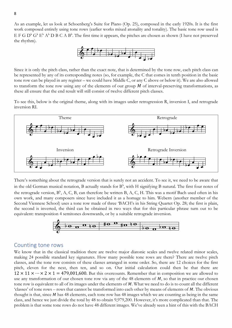
As an example, let us look at Schoenberg’s Suite for Piano (Op. 25), composed in the early 1920s. It is the first work composed entirely using tone rows (earlier works mixed atonality and tonality). The basic tone row used is
E F G D♭ G♭ E♭ A♭ D B C A B♭. The first time it appears, the pitches are chosen as shown (I have not preserved the rhythm).
'&=[-=\V=êZ=!=æV=äT=çW=S!=X=R=P=áQ! Since it is only the pitch class, rather than the exact note, that is determined by the tone row, each pitch class can be represented by any of its corresponding notes (so, for example, the C that comes in tenth position in the basic tone row can be played in any register – we could have Middle C, or any C above or below it). We are also allowed
to transform the tone row using any of the elements of our group 𝑀 of interval-preserving transformations, as these all ensure that the end result will still consist of twelve different pitch classes. To see this, below is the original theme, along with its images under retrogression R, inversion I, and retrograde inversion RI.
There’s something about the retrograde version that is surely not an accident. To see it, we need to be aware that
in the old German musical notation, B actually stands for B♭, with H signifying B natural. The first four notes of
the retrograde version, B♭, A, C, B, can therefore be written B, A, C, H. This was a motif Bach used often in his own work, and many composers since have included it as a homage to him. Webern (another member of the Second Viennese School) uses a tone row made of three ‘BACH’s in his String Quartet Op. 28; the first is plain, the second is inverted, the third can be obtained in two ways that for this particular phrase turn out to be equivalent: transposition 4 semitones downwards, or by a suitable retrograde inversion.
'&==èx=w=y=øx!==Úz={=Ùy=úz!=æv=u=çw=öv!
Counting tone rows We know that in the classical tradition there are twelve major diatonic scales and twelve related minor scales, making 24 possible standard key signatures. How many possible tone rows are there? There are twelve pitch classes, and the tone row consists of these classes arranged in some order. So, there are 12 choices for the first pitch, eleven for the next, then ten, and so on. Our initial calculation could then be that there are
12 × 11 × ⋯ × 2 × 1 = 479,001,600. But this overcounts. Remember that in composition we are allowed to use any transformation of our chosen tone row via any of the 48 elements of 𝑀, so that in practice our chosen tone row is equivalent to all of its images under the elements of 𝑀. What we need to do is to count all the different ‘classes’ of tone rows – rows that cannot be transformed into each other by means of elements of 𝑀. The obvious thought is that, since 𝑀 has 48 elements, each tone row has 48 images which we are counting as being in the same class, and hence we just divide the total by 48 to obtain 9,979,200. However, it’s more complicated than that. The problem is that some tone rows do not have 48 different images. We’ve already seen a hint of this with the BACH
9
motif, though that was only four notes. It turns out that if we denote by 𝑊 the Webern tone row mentioned above, we have 𝑇−1𝑅(𝑊) = 𝐼(𝑊).4
What hope do we have of analysing 479 million tone rows to see which ones are equivalent? Luckily, group theory comes to the rescue in the form of something called Burnside’s Lemma, named after William Burnside, a Victorian mathematician who was Professor of Mathematics at the Royal Naval College in Greenwich. It says the following: suppose you have a group 𝐺 whose elements permute the elements of some set 𝑋 (in our case the group is 𝑀, and its elements permute the set of all possible tone rows). For 𝑔 in 𝐺, write Fix(𝑔) for the set of elements of 𝑋 that are left fixed by 𝑔. (For example, with Webern’s tone row 𝑊, since 𝑇−1𝑅(𝑊) = 𝐼(𝑊), we have 𝐼𝑇−1𝑅(𝑊) = 𝑊.
Thus, 𝑊 ∈ Fix(𝐼𝑇−1𝑅)). Burnside’s Lemma says that the total number of different classes of elements of 𝑋 (where elements are considered to be in the same class if they are permutations of one another via elements of the group G), is given by
1
|𝐺|∑ |Fix
𝑔∈𝐺
(g)|
In other words, instead of working through 479 million tone rows to see which ones are really the same, we can work through just the 48 elements of 𝑀 and work out how many tone rows they fix. Most do not fix any tone
rows. For example, any non-zero transposition results in a different first note, so |𝐹𝑖𝑥(𝑇𝑛)| = 0 unless 𝑛 = 0,
in which case |Fix(𝑇𝑛)| = 479,001,600. The inversion 𝐼𝑝 fixes only the pitch classes 𝑝 and 𝑝 + 6 (and these
will only actually be pitch classes if 𝑝 is an integer, rather than a half-integer). This is because 𝐼𝑝(𝑥) = 2𝑝 − 𝑥, and
𝑥 is in the same pitch class as 2𝑝 − 𝑥 only when these pitches are the same or differ by a multiple of 12 semitones (one octave). That is, if 2𝑝 − 2𝑥 is a multiple of 12. Since the tone row cannot contain any repeats, at most two of its notes are fixed by any inversion, meaning the tone row as a whole certainly cannot be fixed. Thus, |𝐹𝑖𝑥(𝑇𝑛𝐼)| = 0 for all 𝑛. We have seen this interval p to p+6 before – it is known as a tritone; exactly half an
octave, or three whole tones, for example from C to F♯. If 𝑇𝑛𝑅 fixed any tone row, then doing it twice would also fix that tone row. But 𝑇𝑛𝑅𝑇𝑛𝑅 = 𝑇2𝑛. So, the only possibilities are 𝑛 = 0 and 𝑛 = 6. If 𝑛 = 0, we just get plain retrogression, which clearly cannot fix any tone row. If 𝑛 = 6, then we are very constrained. Writing the notes (or strictly speaking the pitch classes) as 𝑝1 to 𝑝12, we have that 𝑝12 = 𝑝1 + 6, 𝑝11 = 𝑝2 + 6, and so on. In other words, determining 𝑝1 to 𝑝6 determines the whole tone row. We have twelve choices for 𝑝1, and then 𝑝12 must be the corresponding tritone. That leaves ten choices for 𝑝2, eight choices for 𝑝3 and so on. Combining, we get 12 × 10 × 8 × 6 × 4 × 2 = 46,080 tone rows that are fixed by 𝑇6𝑅. The remaining elements of 𝑀 are the retrograde inversions 𝐼𝑝𝑅. If 𝐼𝑝 fixes any pitch class, then suppose that the class is note 𝑝𝑚 in the tone row. We
will have 𝐼𝑝𝑅(𝑝12−𝑚) = 𝐼𝑝(𝑝𝑚) = 𝑝𝑚, which implies that 𝑝12−𝑚 = 𝑝𝑚, contradicting the fact that all notes in a
tone row are different. The only remaining cases are where the inversion in question does not fix any pitch class – this occurs when 𝑝 is not an integer. That is, when 2𝑝 is an odd integer. We are left with six cases: 𝑝 = 1, 3, 5, 7, 9 or 11. In this case, we can have fixed rows. The final six notes are determined by our choice of the first six notes, as with the retrograde case. Here, for example, 𝑝12 = 𝐼𝑝𝑅(𝑝12) = 𝐼𝑝(𝑝1) = 2𝑝 − 𝑝1. So again we have 46,080 tone
rows. In summary, then, the identity element 𝑇0 fixes all tone rows, 𝑇6𝑅 and six of the retrograde inversions fix 46,080 tone rows, and no other element of 𝑀 fixes any tone row. In Burnside’s Lemma, then, we get that the number of different classes of tone rows is
1
|𝑀|∑ |Fix
𝑔∈𝑀
(g)| =1
48(479,001,600 + 7 × 46,080) = 9,985,920.
This fact about tone rows was first proved by a mathematician called David Reiner, so we should perhaps call it Reiner’s Theorem. For a more in-depth discussion, including a proof of Burnside’s Lemma, see Chapter 9 of [8]. Once you have chosen your twelve-tone row, there does still remain the task of actually composing a piece of music. The twelve-tone row imposes a challenging constraint, but there is still an infinite variety of paths to follow;
4 If we stick to our earlier arbitrary decision to set the pitch of G♯ as 0, and writing everything modulo 12 as an integer between 1 and 12, then the pitch classes of the original 𝑊 are 2, 1, 4, 3, 7, 8, 5, 6, 10, 9, 12, 11. Both 𝑇−1(𝑅(𝑊)) and 𝐼(𝑊) equal 10, 11, 8, 9, 5, 4, 7, 6, 2, 3, 12, 1.
10
not only with the many inversions, retrogressions and transpositions that are possible, but also in the choice of dynamics, duration of notes, juxtaposition of voices and so on. There were experiments in what is called total serialism, where more or less every aspect of the music is determined by formal structures. The apotheosis, or perhaps nadir, of this idea, was in Pierre Boulez’s 1952 work Structures, for two pianos. The starting point for Boulez was the tone row that his former teacher Olivier Messiaen had used in his 1949 piano work Modes de Valeurs et d’intensités. Messiaen had himself explored the ideas of total serialism in this work but did not take them to anything like the extremes that Boulez did. Boulez took the basic tone row, numbered its pitch classes 1 to 12, in order of appearance, and made two 12 by 12 grids of numbers to represent all 48 images under our group 𝑀 (the tone row used does have 48 different images in this case). The rows of the first grid, the ‘prime’ matrix or P-matrix, read forwards, consist of all the transpositions, from 0 to 11 semitones, and read backwards consist of the retrogrades of these transpositions. The rows of the second grid, (the ‘I-matrix’) read forwards, give you all the inversions, and read backwards give you the retrograde inversions. The order in which the rows are to be used in the music is determined by these grids too. Piano 1, for example, plays the rows of the P-matrix, in the order given by the first row of the I matrix. So those are the notes. The two grids also determined the durations of notes. The row 7, 1, 10, 3, … would give notes of duration 7, 1, 10, 3, … demisemiquavers. That is, the first note would last 7/8 of a crotchet beat, and so on. As if that is not enough, to each number 1 to 12, Boulez assigned both a dynamic instruction (the volume at which to play) and a ‘mode of attack’ to tell you how to play the note – things like staccato or legato. The notes played by Piano 1 had dynamics and mode of attack derived by reading the P-matrix diagonally; for Piano 2 the I-matrix was used. For more detail, see the essay by Jonathan Cross in [9]. Apart from a few things like where to put the rests, everything is pre-determined, leaving very little room for free compositional choice. With a very highly structured system, there is always a risk that the intellectual pleasure of fitting the pieces together outweighs the main goal of making good art. It may be fun completing a Sudoku puzzle, but nobody wants to listen to the completed grid being read out! So why take this system to its logical extent in this way? We must remember the context in which this work was being created. In a 2011 interview [10] a few years before his death, Boulez explained “It was the period. It was immediately after the war - 1945, 1946 - and we wanted a tabula rasa. We were ready to go. People after the war, when they found a good beat or a good jacket, they’d say, “Oh, that was exactly like before the war!” And in music it was exactly the same [..]. We wanted to do something new. So in Structures, Book I (1951–52), where the responsibility of the composer is practically absent, I was extreme on purpose. Had computers existed at that time I would have put the data through them and made the piece that way. But I did it by hand. I was myself a small and very primitive computer. It was a demonstration through the absurd.” He describes the work as a turning point, after which he moved away from strict serialism. When asked if he would rather the piece were not played any more, his response was, “I am not terribly eager to listen to it. But for me it was an experience that was absolutely necessary.”
Conscious use of mathematical forms in music We have not yet addressed the question of whether composers make explicit use of mathematical structures like groups in their composition. The answer is that yes, some do. We will give a handful of examples.
Sets and Groups The American composer Milton Babbitt deserves a mention purely because he is, as far as I know, the only composer who also has a theorem named after him: Babbitt’s Theorem. It states the following: Given any set of tones, the multiplicity of occurrence of a given interval in the set determines the number of tones in common between that set and its transpositions by that interval. In other words, if you have a musical phrase, and you look at the collection of intervals between all possible pairs 𝑝 and 𝑞 of pitches in that phrase, then if an interval of, say, 5 semitones occurs between three pairs of pitches, you can deduce that transposing the phrase by 5 semitones will create a phrase that has exactly three tones in common with the original phrase. This naturally leads to the concept of ‘difference sets’, which are sets in which each possible difference between pairs of numbers (in some suitable range) occurs exactly once. One near-miss example is the set C, D, F, F sharp, or 1, 3, 6, 7. Every possible interval occurs exactly once, except for the tritone interval which occurs twice (once as the interval between 1 and 7 and once as the interval between 7 and 1; if a tritone interval occurs at all, it must occur at least twice because of this symmetry). Therefore, transpositions of this phrase will always intersect the original phrase in at least one tone. Babbitt has written
11
extensively about the use of sets and groups in the writing of music – the interested reader should consult, for example, his article Set Structure as a Compositional Determinant [11].
Magic Squares The British composer Peter Maxwell Davies made extensive use of magic squares in works such as Ave maris stella (1975) and A mirror of whitening light (1976-7). In these compositions, the starting points were Gregorian chants, which were ‘processed’ through magic squares. For example, in A mirror of whitening light, the chant used was called Veni Sancti Spiritus. Maxwell Davies took the first eight different notes from the start of the chant (slightly modifying a couple of repetitions by a semitone to make them different, and missing out some repetitions). The notes of this modified them were numbered 1 to 8 and became the first row of an 8 by 8 square. Row 2 was Row 1 transposed such that it started on note 2 of the theme; the resulting notes were numbered 9 to 16. Row 3 was Row 1 transposed such that it started on note 3 of the theme, and so on. The outcome was that to each number 1 to 64, a specific pitch class had been associated. He then used this correspondence to label the numbers in an 8 by 8 magic square called the Magic Square of Mercury, with their corresponding notes. The idea was that the theme had been purified and refined by means of the alchemical transition through the magic square. The original theme is there somewhere, because the process is in theory reversible. The music is then composed by following paths through the magic square. The work begins with the sequence of notes along the top row of the square,
from left to right (C, A, B♭, F♯, D, D, C♯, G). The paths can be rows, columns, diagonals, even spirals, so there is plenty of choice. The durations of the notes were also obtained from the magic square through a different process. There is a more detailed discussion of this, including the actual magic square used and an excerpt from the score, in Chapter 8 of [9]. Of course, a listener is not going to ‘hear’ a magic square, nor, indeed, to intuit the original plainchant theme. But you do hear a clearly structured piece of music, not just a random noise. The point is that the numbers and the structure were key to the process of composition – they gave the composer the building blocks. It is, of course, how we arrange the building blocks that makes the difference between noise and music.
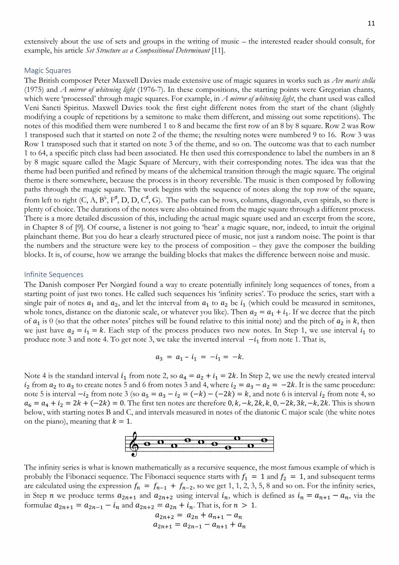
Infinite Sequences The Danish composer Per Nørgård found a way to create potentially infinitely long sequences of tones, from a starting point of just two tones. He called such sequences his ‘infinity series’. To produce the series, start with a single pair of notes 𝑎1 and 𝑎2, and let the interval from 𝑎1 to 𝑎2 be 𝑖1 (which could be measured in semitones, whole tones, distance on the diatonic scale, or whatever you like). Then 𝑎2 = 𝑎1 + 𝑖1. If we decree that the pitch of 𝑎1 is 0 (so that the other notes’ pitches will be found relative to this initial note) and the pitch of 𝑎2 is 𝑘, then we just have 𝑎2 = 𝑖1 = 𝑘. Each step of the process produces two new notes. In Step 1, we use interval 𝑖1 to produce note 3 and note 4. To get note 3, we take the inverted interval −𝑖1 from note 1. That is,
𝑎3 = 𝑎1 – 𝑖1 = −𝑖1 = −𝑘.
Note 4 is the standard interval 𝑖1 from note 2, so 𝑎4 = 𝑎2 + 𝑖1 = 2𝑘. In Step 2, we use the newly created interval 𝑖2 from 𝑎2 to 𝑎3 to create notes 5 and 6 from notes 3 and 4, where 𝑖2 = 𝑎3 − 𝑎2 = −2𝑘. It is the same procedure: note 5 is interval −𝑖2 from note 3 (so 𝑎5 = 𝑎3 − 𝑖2 = (−𝑘) − (−2𝑘) = 𝑘, and note 6 is interval 𝑖2 from note 4, so 𝑎6 = 𝑎4 + 𝑖2 = 2𝑘 + (−2𝑘) = 0. The first ten notes are therefore 0, 𝑘, −𝑘, 2𝑘, 𝑘, 0, −2𝑘, 3𝑘, −𝑘, 2𝑘. This is shown below, with starting notes B and C, and intervals measured in notes of the diatonic C major scale (the white notes on the piano), meaning that 𝑘 = 1.
'&=x=y=w=z=y=x=v{=w=z! The infinity series is what is known mathematically as a recursive sequence, the most famous example of which is probably the Fibonacci sequence. The Fibonacci sequence starts with 𝑓1 = 1 and 𝑓2 = 1, and subsequent terms are calculated using the expression 𝑓𝑛 = 𝑓𝑛−1 + 𝑓𝑛−2, so we get 1, 1, 2, 3, 5, 8 and so on. For the infinity series,
in Step 𝑛 we produce terms 𝑎2𝑛+1 and 𝑎2𝑛+2 using interval 𝑖𝑛, which is defined as 𝑖𝑛 = 𝑎𝑛+1 − 𝑎𝑛, via the
formulae 𝑎2𝑛+1 = 𝑎2𝑛−1 − 𝑖𝑛 and 𝑎2𝑛+2 = 𝑎2𝑛 + 𝑖𝑛. That is, for 𝑛 > 1.
𝑎2𝑛+2 = 𝑎2𝑛 + 𝑎𝑛+1 − 𝑎𝑛 𝑎2𝑛+1 = 𝑎2𝑛−1 − 𝑎𝑛+1 + 𝑎𝑛
12
Per Nørgård has used the infinity series in much of his work since the 1960s. Although the process is entirely deterministic, the effect is of a sequence oscillating in what appears to be a random way. In his compositions, for example the Second Symphony, he uses an infinity series starting at the notes G and A, played at different speeds by different instruments, so that different parts of the orchestra are doing the same things at both large and small scale.
Fractals The idea of the same things being replicated at both large and small scale is reminiscent of the mathematical idea of a fractal. One composer who has used what are called fractal generators in her music is the Finnish composer Kaija Saariaho. Incidentally, she was born on October 14th 1952, so the original date of this lecture, October 13th 2020, is just one day before her birthday. She is a hugely influential innovator in blending electronic music with live performance by instrumentalists. In 2019, BBC Music Magazine surveyed 174 composers, asking them to vote for their top five composers of all time, to create a top 50 list, which makes for a fun conversational starting point. Saariaho was the highest ranking composer still living, coming in at 17th on the list of all-time greats. (The top ten, in order, were J.S. Bach, Stravinsky, Beethoven, Mozart, Debussy, Ligeti, Mahler, Wagner, Ravel and Monteverdi.) Saariaho incorporates computer programs in the creation of her music, such as in the Jardin Secret trilogy, made in the mid 1980s. Nymphéa (Jardin secret III) (1987), a piece for string quartet and electronics, commissioned for the Kronos quartet (in which the musicians also whisper words of a poem during the performance), was partially written with the aid of a fractal generator. In the programme notes for the premiere, Saariaho wrote: ‘In preparing the musical material of the piece, I have used the computer in several ways. The basis of the entire harmonic structure is provided by complex cello sounds that I have analysed with the computer. The basic material for the rhythmic and melodic transformations are computer-calculated in which the musical motifs gradually convert, recurring again and again.’ Fractal music in essence is music that has this self-similarity at different scales. Probably the most famous fractal images come from the Mandelbrot set, which is produced by a process of iterating a given function at each point on a graph; the point is then coloured according to how quickly the value increases; if it does not diverge to infinity the point is coloured black. Fractal sequences also exist, and it is these that are used in fractal generators, to produce infinite sequences of numbers which can be converted into note pitches, durations, or anything else that forms part of the performance. An important example of such a sequence, which is incorporated into many fractal generators, is based on the so-called Thue-Morse sequence (discovered independently by mathematicians Axel Thue and Marston Morse). To create it, you first write down the positive integers 1, 2, 3, 4 and so on, in binary:
The sequence we want is then the sequence of sums of digits of these binary numbers
1, 1, 2, 1, 2, 2, 3, 1, 2, 2, …
What is amazing about this sequence is that if we just pull out the alternate terms starting from the second term, we get
1, 1, 2, 1, 2… In other words, we get exactly the same sequence back again!5 So the sequence contains itself, infinitely many times. That means that a musical composition created using this sequence would contain copies of itself – a true fractal composition. Curiously enough, if you program a computer to draw a path of 𝑛 stages by moving forward one step at stage 𝑛 if 𝑛 is odd, and turning 120 degrees clockwise if 𝑛 is even, then the resulting path, as 𝑛 tends to infinity, converges to the Koch snowflake curve!
5 It’s actually more standard to define the Thue-Morse sequence as this sequence but replacing every even number with 0 and every odd number with 1, but the same fractal property holds in both cases.
13
Probability and Randomness Several composers have used elements of chance in either the composition or the instructions for playing their works. In his work Music of Changes, John Cage introduced randomness by tossing coins, interpreting the results using twenty-six different charts to determine various aspects of the music. Iannis Xenakis was much more mathematically astute, and used a wide variety of mathematical structures and techniques in his composition. Xenakis started out as an engineer, but grew interested in both music and architecture. He studied under Messiaen, who reported telling the young Xenakis, ‘you have the good fortune of being Greek, of being an architect and having studied special mathematics. Take advantage of these things. Do them in your music’. Indeed, Xenakis’s early work Metastasis incorporates, in the form of sweeping glissandi, what look in the score very similar to curves he used in his architectural designs. Writing about this in his book Formalized music: thought and mathematics in composition [12], he wrote: ‘If glissandi are long and sufficiently interlaced, we obtain sonic spaces of continuous evolution. It is possible to produce ruled surfaces by drawing the glissandi as straight lines. I performed this experiment with Metastasis [premiered 1955]. Several years later, when the architect Le Corbusier, whose collaborator I was, asked me to suggest a design for the architecture of the Philips Pavilion in Brussels, my inspiration was pin-pointed by the experiment with Metastasis. Thus I believe that on this occasion music and architecture found an intimate connection’. Xenakis has used game theory, set theory and group theory in his work, among other things. He has described his work using probabilistic or statistical techniques as stochastic music. Brownian motion, for instance, has formed the basis for several of his works, including N'Shirna, meaning ‘breath’ or ‘spirit’ in Hebrew; for two voices, two French Horns, two trombones and a ‘cello. The overarching idea here is that the behaviour of very large collections of objects (such as gas molecules) can behave predictably, or appear to have a designed structure, while individual members of the collection are behaving essentially randomly, a behaviour modelled by so-called ‘random walks’, or Brownian motion. Similarly, the path of a musical theme can be generated by using a random walk model. Another use of statistical techniques was to use a probability distribution to generate the number of times specific notes should appear in the different instruments’ parts. Xenakis chose the Poisson distribution, which is a distribution used to model rare events, for Achorripsis. If we
suppose that the mean average number of events per unit time is 𝜆, then the probability 𝑃𝑘 that the event will
happen 𝑘 times in that unit time is given by 𝑃𝑘 =𝜆𝑘
𝑘!𝑒−𝜆. The events are described by Xenakis as ‘clouds of sound’,
which is more poetic than helpful, it has to be said. He divides the performance into 196 cells, representing 28 units of time for each of seven instruments. The number of these cells in which, say, two events happen, is then 196𝑃2, which, setting as Xenakis does 𝜆 = 0.6, gives 19, to the nearest integer. Therefore, he ensures that in 19 of the cells, two ‘clouds of sound’ occur. To find out more about what constitutes a cloud of sound, you will need to listen to the music! Finally, we turn to that well-known proponent of probabilistic precepts in modern music, Joseph Haydn. In about 1790, a game went on sale, promising to help you, the amateur musician, compose “un infinito numero di minuette trio” – an infinite number of minuet trios (a kind of piano piece). The process is described in Chapter 6 of Harkleroad [13]. Essentially, Haydn (or at least that was the claim of the publishers), composed six sixteen-bar pieces, in such a way that at each bar, any one of the six alternatives for that bar will sound good. So, for bar 1 of your minuet, you roll a die, and if you roll a 3, say, then you play bar 1 of piece 3. Then if you roll a 6, you next play bar 2 of piece 6, and so on. Of course, the claim that there are infinitely many minuets to be composed in this way is false. In fact, assuming all the corresponding bars of each piece are really different, then there will be
sixteen consecutive choices from six options, and so there will be a mere 616 possible minuets. To make matters worse, Haydn (if it was he) used the same final bar in four of the six pieces, and the same eighth bar in three, so
the exact number of possibilities is 614 × 4 × 3 = 940,369,969,152, just short of a trillion. Harkleroad calculates that a complete continuous performance of these minuet trios would take around 900,000 years (or double that if you follow the direction in the music to play the trio through twice).
Summary I see the use of mathematics in musical composition as the continuation of what has always happened in music – the voluntary imposition of structure to act as a creative spur. An early example is the soggato cavato technique, used by Renaissance composer Josquin Des Prez, where you take a phrase, match its vowels with the vowels in the set of note names (at that time not do but ut, re, mi, fa, sol, la), and use this to create a fixed musical phrase, the cantus firmus, around which the composition would be based. It would be almost impossible to derive the original phrase
14
from such a transformation, but it is the underlying cipher behind the music. This feels in spirit rather reminiscent of processing a melody through a magic square. The original information is obscured, but the process has created an architecture for the composition. Constraint can be a spur to creativity. Too much constraint traps you in a rigid edifice from which it is hard to escape. In the most successful works that incorporate mathematical techniques or structures, they serve the composer, rather than the other way around. As Schoenberg famously said, ‘one has to follow the basic set; but, nevertheless, one composes as freely as before’, and, ‘my works are 12-tone compositions, not 12-tone compositions’. We need a structure, or the ‘music’ is just noise. But too much structure can lead either to sterility or something that sounds, because the artist has so little input, almost random. We cannot ‘hear’ a magic square. What we hear is a clearly structured piece of music, not just a random noise. The point is that the numbers and the structure were key to the process of composition – they gave the composer the building blocks. It is, of course, how we arrange the building blocks that makes the difference between noise and music. Mathematical structures are ever-present in music, but the composer should always have the upper hand!
Further Reading
[1] M. Church, The Other Classical Musics: Fifteen Great Traditions, Boydell Press, 2015.
[2] T. Levin, The Hundred Thousand Fools of God: Musical Travels in Central Asia (and Queens, New York), Indiana University Press, 1997.
[3] B. Nettl and T. Rommen, Excursions in World Music, Routledge, 2017.
[4] M. Tenzer, Balinese Gamelan Music, Tuttle Publishing, 2011.
[5] V. Wilmer, As Serious as Your Life: Black Music and the Free Jazz Revolution, 1957-1977, Serpent's Tail Classics, 2018.
[6] S. Bruhn, “Symmetry and dissymmetry in Paul Hindemith's Ludus Tonalis,” Symmetry: Culture and Science, vol. 7, no. 2, p. 116–132, 1996.
[7] I. Xenakis, R. Brown and J. Rahn, “Xenakis on Xenakis,” Perspectives of New Music, vol. 25, no. 1, pp. 16-63, Winter-Summer 1987.
[8] D. Benson, Music: A Mathematical Offering, Cambridge: Cambridge University Press, 2006.
[9] J. Fauvel, R. Flood and R. Wilson, Music and Mathematics, Oxford: Oxford University Press, 2003.
[10] I. Toronyi-Lalic, “theartsdesk Q&A: Composer Pierre Boulez,” 7 January 2020. [Online]. Available: https://www.theartsdesk.com/classical-music/theartsdesk-qa-composer-pierre-boulez. [Accessed 24/7/20].
[11] M. Babbitt, “Set Structure as a Compositional Determinant,” Journal of Music Theory, vol. 5, no. 1, pp. 72-94, 1961.
[12] I. Xenakis, Formalized music: thought and mathematics in composition, Pendragon Press, 1992.
[13] L. Harkleroad, The Math Behind the Music, Cambridge: Cambridge University Press, 2006.
[14] E. Maor, Music by the Numbers: From Pythagoras to Schoenberg, Princeton University Press, 2018.
Further Listening
• The palindromic rondeau by Guillaume de Machaut, Ma fin est mon commencement. https://www.youtube.com/watch?v=dcfPr4IN2MM
• Hadyn’s palindromic Minuet ‘al roverso’ (from his Symphony No. 47) – the Trio is also a palindrome. https://www.youtube.com/watch?v=zF7xXkptLVc
• Mozart’s Der Spiegel played on violin and mandolin https://www.youtube.com/watch?v=lsqPzVrSigw
• Boulez’s Structures Ia for two pianos (if you dare!) https://www.youtube.com/watch?v=-Tx7oSiM42E Try his 1945 work Douze Notations for piano for a more ‘accessible’ experience. https://www.youtube.com/watch?v=CJG38iQ9d7I