36
Economics 250aLecture 14Gender Disparities in the Labor Market
Reading ListAs with the topic of racial disparities, there is a huge literature on gender-
related di�erences in the labor market. Here are some (relatively) recent papersthat strike me as useful.
A. Useful overviews:1) Joseph Altonji and Rebecca Blank. "Race and Gender in the Labor
Market." In O. Ashenfelter and D. Card, Handbook of Labor Economics volume3. Elsevier, 1999.
2) Marianne Bertrand. �New Perspectives on Gender.� In Orley Ashenfelterand David Card (editors) Handbook of Labor Economics, Vol. 4b. Amsterdam:Elsevier. 2011. pp. 1543-1590.
3) O'Neill, June, and Dave O'Neill. 2006 "What Do Wage Di�erentials TellUs about Labor Market Discrimination?" Research in Labor Economics 24: 293-357. This is an example of �old school Chicago� style analysis, pushed to thelimit (and beyond).
4) Fancine Blau and Lawrence Kahn. 2016. �The Gender Wage Gap: Extent,Trends, and Explanations.�NBER Working Paper No. 21913.
B. Human capitalJoseph G. Altonji, Erica Blom and Costas Meghir. 2012. �Heterogeneity
in Human Capital Investments: High School Curriculum, College Major, andCareers" Annual Review of Economics, 4(1): 185-223. Get the NBER Version(WP #17985) for the extra tables and materials.
Casey B. Mulligan and Yona Rubinstein. 2008. �Selection, Investment, andWomen's Relative Wages over Time� Quarterly Journal of Economics, 123 (3):1061-1110. This is an extended analysis of the potential e�ect of �selection bias�induced by the lower participation rate of women than men.
Manning, Alan, and Joanna Swa�eld. 2008. "The gender gap in early-career wage growth." Economic Journal 118: 983-1024. This is a nice, carefulanalysis of the causes of the widening wage gap with experience.
C. Employer DiscriminationOne interesting thing you will notice right away is that very few recent papers
try to measure �discrimination� or model/discuss the ways that discriminationworks, or could work. Economists appear to have either �moved on� or �givenup� on discrimination.
Peter Kuhn. 1987. �Sex Discrimination in Labor Markets: The Role ofStatistical Evidence.� American Economic Review, 77(4): 567-583. This paperuses survey information that asked women whether they felt that they werediscriminated against, and compares responses to this question to estimates ofthe wage gap for the same person.
Michael Ransom and Ronald G. Oaxaca. 2005. �Intra�rm mobility and sexdi�erences in pay.� Industrial & Labor Relations Review. 2005. This is one one
1
of the few papers to carefully document how an employer set up �occupations�to enforce gender segregation and facilitate lower pay for women.
Goldin, Claudia and Cecilia Rouse. 2000. "Orchestrating Impartiality: TheImpact Of 'Blind' Auditions On Female Musicians," American Economic Re-
view, 90(4): 715-741.David Neumark, Roy Bank and Kyle Van Nort. 1996 �Sex Discrimination in
Restaurant Hiring: An Audit Study� Quarterly Journal of Economics 111 (3):915-941. This is an older audit study. By today's standards it has a number ofweaknesses, but there are relatively few recent studies focused on gender.
D. BargainingBabcock, Linda, and Sara Laschever. Women don't ask: Negotiation and the
gender divide. Princeton University Press, 2009.Jenny Säve-Söderbergh. �Are Women Asking for Low Wages? Gender Dif-
ferences in Wage Bargaining Strategies and Ensuing Bargaining Success. Un-published Paper, Stockholm University, Swedish Inst. for Social Research.
David Card, Ana Rute Cardoso, and Patrick Kline. 2016. �Bargaining,Sorting, and the Gender Wage Gap: Quantifying the Impact of Firms on theRelative Pay of Women.� Quarterly Journal of Economics, 131(2): 633-686.
E. Supply-Based ModelsBowlus, Audra J., 1997. A search interpretation of male�female wage di�er-
entials. Journal of Labor Economics 15, 625�657.Barth, Erling, and Harald Dale-Olsen, "Monopsonistic Discrimination, Worker
Turnover, and the Gender Wage Gap," IZA Discussion Paper No. 3930, 2009.David Card, Ana Rute Cardoso, Joerg Heining and Patrick Kline. �Firms
and Labor Market Inequality: Evidence and Some Theory�. NBER WorkingPaper 22850, November 2016.
F. Compensating Di�erences (Broadly construed)a. hours-based stories
Bertrand, Marianne, Claudia Goldin, and Lawrence F. Katz. 2010. "Dy-namics of the Gender Gap for Young Professionals in the Financial and Corpo-rate Sectors." American Economic Journal: Applied Economics, 2(3): 228-55.
Goldin, Claudia. 2014. �A Grand Gender Convergence: Its Last Chapter.�American Economic Review 104(4): 1091-1119.
b. avoiding competition
Muriel Niederle and Lise Vesterlund. 2007. �Do Women Shy Away fromCompetition? Do Men Compete Too Much?� Quarterly Journal of Economics
122(3): 1067-1101.Je�rey A. Flory, Andreas Leibbrandt, and John A. List. 2015 �Do Compet-
itive Workplaces Deter Female Workers? A Large-Scale Natural Field Experi-ment on Job Entry Decisions.� Review of Economic Studies 82 (1): 122-155
G. Other Pyschological Storiesa. Fear of Earning More than One's Spouse
Marianne Bertrand, Emir Kamenica, and Jessica Pan. 2015 �Gender Identityand Relative Income within Households� Quarterly Journal of Economics (2015)
2

130 (2): 571-614. In this paper, it is argued that married women have a strongaversion to earning more than their spouse. They argue that this exerts anegative e�ect on women's earnings!
b. Gender Indentity
Nicole M. Fortin. 2008. �The Gender Wage Gap among Young Adults inthe United States The Importance of Money versus People.� Journal of HumanResources 43(4): 884-918
3
66
Notes: Updated version of Figure 7-2 from Blau, Ferber, and Winkler (2014); for additional information on references, see p. 148. Workers aged 16 and over from 1979 onward, and 14 and over prior to 1979.
55
60
65
70
75
80
85
1955
1960
1965
1970
1975
1980
1985
1990
1995
2000
2005
2010
Earn
ings
Rat
io (P
erce
nt)
Year
Figure 1: Gender Earnings Ratios of Full-Time Workers 1955-2014
Weekly Annual (Full Year)
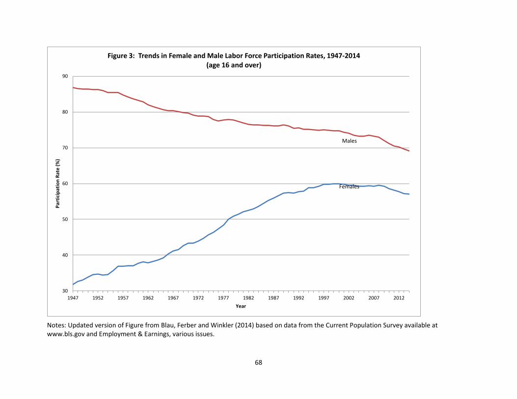
68
Notes: Updated version of Figure from Blau, Ferber and Winkler (2014) based on data from the Current Population Survey available at www.bls.gov and Employment & Earnings, various issues.
30
40
50
60
70
80
90
1947 1952 1957 1962 1967 1972 1977 1982 1987 1992 1997 2002 2007 2012
Part
icip
atio
n Ra
te (%
)
Year
Figure 3: Trends in Female and Male Labor Force Participation Rates, 1947-2014(age 16 and over)
Males
Females
69
Table 1: Unadjusted Female/Male Log Hourly Wage Ratios, Full Time Workers
Year Men Women Mean 10th Percentile 50th Percentile 90th Percentile
1980 2282 1491 62.1% 64.8% 60.1% 62.4%1989 2617 2068 74.0% 76.3% 72.4% 74.6%1998 2391 2146 77.2% 80.3% 79.8% 73.8%2010 2368 2456 79.3% 81.5% 82.4% 73.9%
1980 21428 13484 63.5% 68.7% 61.9% 64.3%1989 21343 16487 72.4% 78.1% 72.2% 71.4%1998 17520 14231 77.1% 81.3% 76.2% 76.1%2010 24229 20718 82.3% 87.6% 82.2% 76.6%
Notes: Sample includes nonfarm wage and salary workers age 25-64 with atleast 26 weeks of employment. Entries are exp(D), where D is the femalemean log wage, 10th, 50th or 90th percentile log wage minus thecorresponding male log wage.
Sample Size
Panel Study of Income Dynamic (PSID)
March Current Populations Survey (CPS)
70
Table 2: Schooling and Actual Full Time Work Experience by Gender, PSID
Year Men Women Men-Women
Years of Schooling1981 13.3 13.2 0.21990 13.8 13.7 0.01999 14.2 14.3 -0.12011 14.3 14.5 -0.2
Bachelor's Degree Only1981 18.1% 15.3% 2.7%1990 20.0% 17.6% 2.3%1999 23.4% 22.2% 1.2%2011 26.2% 24.7% 1.5%
Advanced Degree1981 10.0% 7.4% 2.5%1990 10.3% 8.7% 1.6%1999 11.7% 10.8% 0.9%2011 12.9% 15.7% -2.8%
Years of Full Time Experience1981 20.3 13.5 6.81990 19.2 14.7 4.51999 19.8 15.9 3.82011 17.8 16.4 1.4
Notes: Sample includes full time nonfarm wage and salary workers age 25-64 with at least 26 weeks of employment.
71
Table 3: Incidence of Managerial or Professional Jobs and Collective Bargaining Coverage by Gender, PSID
Year Men Women Men-Women
Managerial Jobs1981 21.5% 9.2% 12.3%1990 21.1% 10.9% 10.2%1999 21.8% 15.3% 6.5%2011 18.3% 16.2% 2.2%
Professional Jobs1981 17.0% 21.8% -4.8%1990 19.4% 26.1% -6.6%1999 20.4% 26.9% -6.4%2011 21.7% 31.1% -9.4%
"Male" Professional Jobs1981 14.6% 10.1% 4.5%1990 17.3% 14.1% 3.2%1999 17.6% 13.2% 4.4%2011 18.6% 17.8% 0.8%
Collective Bargaining Coverage1981 34.5% 21.1% 13.3%1990 25.4% 19.4% 6.1%1999 21.5% 18.2% 3.3%2011 17.4% 18.9% -1.5%
Notes: Sample includes full time nonfarm wage and salary workers age25-64 with at least 26 weeks of employment. "Male" Professional jobsare professional jobs excluding nurses and K-12 and othernon-college teachers.
72
Table 4: Decomposition of Gender Wage Gap, 1980 and 2010 (PSID)
1980 2010Effect of Gender Gap in Explanatory Variables
Effect of Gender Gap in Explanatory Variables
Variables Log Points
Percent of Gender Gap
Explained Log Points
Percent of Gender Gap
Explained
A. Human Capital Specification
Education Variables 0.0129 2.7% -0.0185 -7.9%Experience Variables 0.1141 23.9% 0.0370 15.9%Region Variables 0.0019 0.4% 0.0003 0.1%Race Variables 0.0076 1.6% 0.0153 6.6%Total Explained 0.1365 28.6% 0.0342 14.8%Total Unexplained Gap 0.3405 71.4% 0.1972 85.2%Total Pay Gap 0.4770 100.0% 0.2314 100.0%
B. Full Specification
Education Variables 0.0123 2.6% -0.0137 -5.9%Experience Variables 0.1005 21.1% 0.0325 14.1%Region Variables 0.0001 0.0% 0.0008 0.3%Race Variables 0.0067 1.4% 0.0099 4.3%Unionization 0.0298 6.2% -0.0030 -1.3%Industry Variables 0.0457 9.6% 0.0407 17.6%Occupation Variables 0.0509 10.7% 0.0762 32.9%Total Explained 0.2459 51.5% 0.1434 62.0%Total Unexplained Gap 0.2312 48.5% 0.0880 38.0%Total Pay Gap 0.4770 100.0% 0.2314 100.0%
Notes: Sample includes full time nonfarm wage and salary workers age 25-64 with at least 26weeks of employment. Entries are the male-female differential in the indicated variablesmultiplied by the current year male log wage coefficients for the corresponding variables. The total unexplained gap is the mean female residual from the male log wage equation.
73
Table 5: Effect of Changes in Explanatory Variables and Male Wage Coefficients on the Change in the Gender Wage Gap, 1980-2010
Base: 1980 Male Wage Equation; 2010 Male-Female Gap in
Explanatory Variables
Base: 2010 Male Wage Equation; 1980 Male-Female Gap in
Explanatory Variables
VariablesHuman Capital Specification
Full Specification
Human Capital Specification
Full Specification
Effect of Changing MeansEducation Variables -0.0219 -0.0219 -0.0461 -0.0343Experience Variables -0.0767 -0.0674 -0.0460 -0.0433Region Variables -0.0058 -0.0030 -0.0004 0.0002Race Variables -0.0018 -0.0017 0.0006 0.0003Unionization -- -0.0331 -- -0.0303Industry Variables -- -0.0080 -- 0.0032Occupation Variables -- -0.0253 -- -0.0369
All X's -0.1062 -0.1603 -0.0920 -0.1411
Effect of Changing Coefficients
Education Variables -0.0095 -0.0041 0.0148 0.0083Experience Variables -0.0004 -0.0006 -0.0310 -0.0246Region Variables 0.0042 0.0037 -0.0011 0.0005Race Variables 0.0096 0.0049 0.0071 0.0030Unionization -- 0.0003 -- -0.0025Industry Variables -- 0.0031 -- -0.0082Occupation Variables -- 0.0506 -- 0.0622
All B's 0.0039 0.0579 -0.0103 0.0386
Effect of Changing Unexplained Gaps -0.1433 -0.1432 -0.1433 -0.1432
Change in the Total Wage Gap -0.2456 -0.2456 -0.2456 -0.2456
Notes: Effect of Changing Means is the change over the 1980-2010 period in the male-female difference in the indicated variables multiplied by the indicated male log wage coefficients for thecorresponding variables. Effect of Changing Coefficients is the the change over the 1980-2010 period in the male wage coefficients for the indicated variables, multiplied by the correspondingmale-female difference in the means of the indicated variables.
Table 9
Gender Wage Gap Among the NLSY Cohort, Ages 35-43 in 2000, Controlling for Different Sets of Explanatory Variables: Results for All Men and Women and
Specified Sub-groups
AllBy Schooling Level Never had a
child and never
marriedHS Grad or less
COL Grad or more
Unadjusted log hourly wage gap -0.235 -0.229 -0.287 0.076 ns
Log wage differential controlling for:
1). Age, SMSA, region and race, schooling, AFQT -0.231 -0.230 -0.244 -0.019 ns
2). Variables in 1) plus life time work experience -0.121 -0.074 -0.182 -0.065 ns
3). Variables in 2) plus L.F. withdrawal due to family responsibilities -0.102 -0.058 -0.155 -0.054 ns
4).Variables in 3) plus class of worker -0.095 -0.060 -0.120 -0.042 ns
5).Variables in 4) plus occupational characteristics -0.084 -0.073 -0.078 -0.013 ns
6). Variables in 5) plus percent female in occupation -0.079 -0.054 -0.078 -0.027 ns
* All female coefficients are significant at the 10% level or lower unless indicated with "ns".
Note: The log wage differentials are partial regression coefficients of a dummy (0,1) variable for "female" from a series of OLS log wage regressions containing the explanatory variables noted. Separate regressions were conducted for each population group shown. For further information on the individual variables included see the text and Table 10.Source: National Longitudinal Survey of Youth (NLSY79) merged with measures of occupational characteristics (3-digit level) from the September 2001 CPS, the CPS March, and the Dictionary of Occupational Titles (1991).
Table 10 Means and Partial Regression Coefficients of Explanatory Variables1) from Separate NLSY Log Wage Regressions
for Men and Women Ages 35-43 in 2000Means Female Male
Female MaleM2 M4 M2 M4
Coef. t-stat Coef. t-stat Coef. t-stat Coef. t-statRace
Hispanic (0,1) 0.182 0.193 0.063 2.57 0.060 2.61 -0.025 -1.02 -0.018 -0.75Black (0,1) 0.316 0.282 0.053 2.42 0.066 3.14 -0.022 -0.92 0.005 0.20
Education and skill level<10 yrs. 0.031 0.052 -0.089 -1.76 -0.078 -1.64 -0.028 -0.65 -0.025 -0.6010-12 yrs (no diploma or GED) * 0.103 0.124 --- --- --- --- --- --- --- ---HS grad (diploma) 0.300 0.326 -0.003 -0.10 -0.008 -0.27 -0.018 -0.65 -0.013 -0.50HS grad (GED) 0.045 0.056 -0.015 -0.34 -0.046 -1.12 0.027 0.63 0.015 0.38
Some college 0.308 0.232 0.090 2.99 0.060 2.09 0.166 5.31 0.123 4.08BA or equiv. degree 0.153 0.155 0.276 7.61 0.216 6.19 0.373 10.23 0.260 7.08MA or equiv. degree 0.053 0.041 0.391 8.49 0.348 7.76 0.562 10.84 0.446 8.62Ph.D or prof. Degree 0.007 0.015 0.758 7.47 0.654 6.71 0.806 10.60 0.639 8.53
AFQT percentile score (x.10) 3.981 4.238 0.042 9.92 0.032 7.84 0.042 9.92 0.029 7.04
L.F. withdrawal due to family responsibilities (0,1) 0.549 0.130 -0.081 -4.16 -0.082 -4.46 -0.080 -3.14 -0.066 -2.74Lifetime Work Experience
Weeks worked in civilian job since age 18 ÷ 52 15.565 17.169 0.030 13.85 0.023 11.13 0.038 12.54 0.034 11.39Weeks worked in military since 1978 ÷ 52 0.062 0.573 0.046 3.53 0.040 3.22 0.025 5.15 0.020 4.46Weeks PT ÷ total weeks workd since age 22 0.137 0.050 -0.203 -4.24 -0.084 -1.81 -0.779 -7.90 -0.540 -5.70
Employment typeGov't employer (0,1) 0.215 0.144 -0.030 -1.50 -0.027 -1.13Non-profit employer (0,1) 0.100 0.049 -0.056 -2.13 -0.121 -3.20
OCC. Characteristics of Person's 3-digit OCC.SVP required in occup. (months) (DOT) 26.961 28.773 0.001 2.44 0.003 5.43Hazards (0,1) (DOT) 0.013 0.084 0.327 4.66 0.131 3.97Fumes (0,1) (DOT) 0.004 0.043 -0.293 -2.27 -0.075 -1.72Noise (0,1) (DOT) 0.080 0.307 0.005 0.18 0.019 0.83Strength (0,1) (DOT) 0.092 0.215 0.011 0.37 -0.049 -1.99Weather extreme (0,1) (DOT) 0.033 0.188 0.120 2.56 0.000 -0.01Prop. using computers (CPS) 0.557 0.415 0.157 2.19 0.045 0.49Prop. using computer for analysis (CPS) 0.143 0.139 0.497 4.62 0.258 2.22Prop. using computer for word proc. (CPS) 0.345 0.236 -0.255 -3.19 -0.007 -0.06Relative rate of transition to unemployment 0.772 1.092 -0.022 -1.11 -0.023 -1.91Relative rate of transition to OLF 1.046 0.789 -0.144 -7.30 -0.073 -3.57% female in OCC. X 0.1. (CPS ORG) 6.348 2.695 0.005 1.08 -0.019 -3.55
Adj. R-Square 0.392 0.464 0.403 0.467Dependent mean (Log Hourly Wage) 2.529 2.764Sample size 2704 26941) Model also controls for age, central city, MSA, region, and occupation missing.* Reference group.Source: National Longitudinal Survey of Youth (NLSY79) merged with measures of occupational characteristics (3-digit level) from the September 2001 CPS, the March CPS, the CPS ORG, and the Dictionary of Occupational Titles (1991).
Table 11
Gender Wage Gap: Decomposition Results (NLSY, 2000)
Using male coefficients Using female coefficients
M1 M2 M3 M4 M1 M2 M3 M4
Log Wage Gap (Male-Female) Attributable to:Age, race, region, central city, MSA 0.0044 0.0112 0.0089 0.0089 0.0040 0.0089 0.0064 0.0064AFQT 0.0132 0.0107 0.0073 0.0074 0.0143 0.0107 0.0081 0.0081Education level -0.0138 -0.0128 -0.0094 -0.0096 -0.0147 -0.0068 -0.0054 -0.0052L.F. withdrawal due to family responsibilities 0.0335 0.0272 0.0277 0.0340 0.0344 0.0343Lifetime work experience 0.1425 0.1135 0.1116 0.0901 0.0649 0.0655Nonprofit, government 0.0088 0.0081 0.0048 0.0050
Occupational characteristics: Investment related
SVP (Specific Vocational Preparation) 0.0062 0.0053 0.0020 0.0021Computer usage 0.0122 -0.0040 -0.0054 -0.0024
Compensating differencesDisamenities (physical) 0.0167 0.0040 0.0252 0.0267Unemployment risk; labor force turnover 0.0116 0.0028 0.0226 0.0259
TYP: % female in occupation 0.0721 -0.0137
Unadjusted log wage gap 0.2351 0.2351 0.2351 0.2351 0.2351 0.2351 0.2351 0.2351Total explained by model 0.0037 0.1851 0.2030 0.2342 0.0036 0.1370 0.1578 0.1526Unexplained log wage gap 0.2314 0.0500 0.0321 0.0009 0.2315 0.0981 0.0773 0.0825
Unadjusted hourly wage ratio (Female/Male) : 79.0 79.0 79.0 79.0 79.0 79.0 79.0 79.0Adjusted hourly wage ratio (Female/Male) : 79.3 95.1 96.8 99.9 79.3 90.7 92.6 92.1
Note: Decomposition results shown are derived from results of separate regressions for men and women. See Table 10 for variable means and coefficients using Model 2 and 4. Wage ratios are based on the exponentiated log hourly wage.Source: National Longitudinal Survey of Youth (NLSY79) merged with measures of occupational characteristics (3-digit level) from the September 2001 CPS, the March CPS, the CPS ORG, and the Dictionary of Occupational Titles (1991).
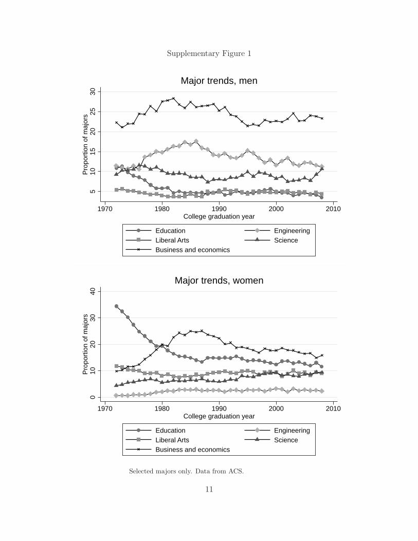
Supplementary Figure 1
510
1520
2530
Pro
porti
on o
f maj
ors
1970 1980 1990 2000 2010College graduation year
Education EngineeringLiberal Arts ScienceBusiness and economics
Major trends, men0
1020
3040
Pro
porti
on o
f maj
ors
1970 1980 1990 2000 2010College graduation year
Education EngineeringLiberal Arts ScienceBusiness and economics
Major trends, women
Selected majors only. Data from ACS.
11
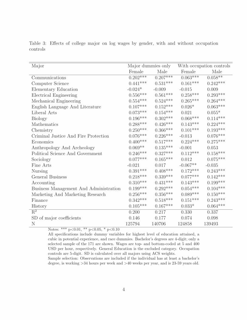
Table 3: Effects of college major on log wages by gender, with and without occupationcontrols
Major Major dummies only With occupation controlsFemale Male Female Male
Communications 0.202*** 0.207*** 0.063*** 0.058**Computer Science 0.441*** 0.531*** 0.161*** 0.242***Elementary Education -0.024* -0.009 -0.015 0.009Electrical Engineering 0.556*** 0.561*** 0.258*** 0.293***Mechanical Engineering 0.554*** 0.524*** 0.265*** 0.264***English Language And Literature 0.107*** 0.152*** 0.026* 0.063***Liberal Arts 0.073*** 0.154*** 0.021 0.055*Biology 0.196*** 0.302*** 0.068*** 0.114***Mathematics 0.288*** 0.426*** 0.143*** 0.224***Chemistry 0.250*** 0.366*** 0.101*** 0.193***Criminal Justice And Fire Protection 0.076*** 0.226*** -0.013 0.076***Economics 0.400*** 0.517*** 0.224*** 0.275***Anthropology And Archeology 0.069** 0.135*** -0.001 0.053Political Science And Government 0.246*** 0.327*** 0.112*** 0.158***Sociology 0.077*** 0.165*** 0.012 0.075***Fine Arts -0.021 0.017 -0.067** -0.035Nursing 0.391*** 0.408*** 0.172*** 0.243***General Business 0.218*** 0.339*** 0.077*** 0.142***Accounting 0.310*** 0.431*** 0.143*** 0.199***Business Management And Administration 0.199*** 0.292*** 0.054*** 0.104***Marketing And Marketing Research 0.256*** 0.356*** 0.089*** 0.150***Finance 0.342*** 0.518*** 0.151*** 0.243***History 0.105*** 0.167*** 0.033* 0.064***R2 0.200 0.217 0.330 0.337SD of major coefficients 0.146 0.177 0.074 0.098N 125794 140706 124858 139493
Notes: *** p<0.01, ** p<0.05, * p<0.10All specifications include dummy variables for highest level of education attained, acubic in potential experience, and race dummies. Bachelor’s degrees are 4-digit; only aselected sample of the 171 are shown. Wages are top- and bottom-coded at 5 and 400USD per hour, respectively. General Education is the excluded category. Occupationcontrols are 5-digit. SD is calculated over all majors using ACS weights.Sample selection: Observations are included if the individual has at least a bachelor’sdegree, is working >34 hours per week and >40 weeks per year, and is 23-59 years old.
4
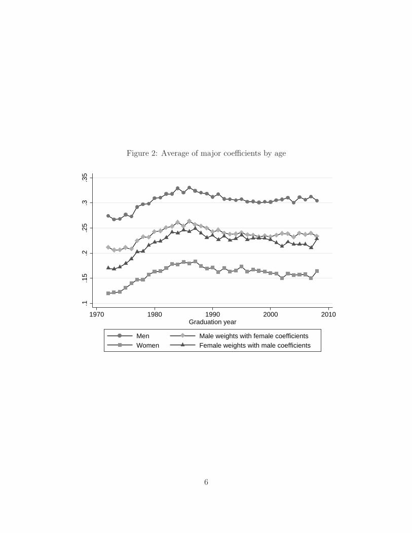
Figure 2: Average of major coefficients by age
.1.1
5.2
.25
.3.3
5
1970 1980 1990 2000 2010Graduation year
Men Male weights with female coefficientsWomen Female weights with male coefficients
6
This content downloaded from 128.32.105.184 on Fri, 18 Nov 2016 06:21:13 UTCAll use subject to http://about.jstor.org/terms
the right-hand side of which is simply two one-period sets of wage growth. One canreadily extend this formula to any value of g in which case it will be given by:
E Dwitð Þ ¼Xg�1
j¼0/ðeit þ jÞ: ð3Þ
Using the specific functional form in (1), this can be written as:
E Dwitð Þ ¼ b0g þ b1Xg�1
j¼0ðeit þ jÞ þ b2
Xg�1
j¼0ðeit þ jÞ2: ð4Þ
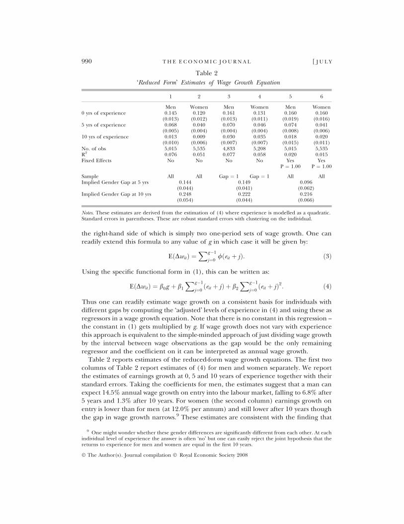
Thus one can readily estimate wage growth on a consistent basis for individuals withdifferent gaps by computing the �adjusted� levels of experience in (4) and using these asregressors in a wage growth equation. Note that there is no constant in this regression –the constant in (1) gets multiplied by g. If wage growth does not vary with experiencethis approach is equivalent to the simple-minded approach of just dividing wage growthby the interval between wage observations as the gap would be the only remainingregressor and the coefficient on it can be interpreted as annual wage growth.
Table 2 reports estimates of the reduced-form wage growth equations. The first twocolumns of Table 2 report estimates of (4) for men and women separately. We reportthe estimates of earnings growth at 0, 5 and 10 years of experience together with theirstandard errors. Taking the coefficients for men, the estimates suggest that a man canexpect 14.5% annual wage growth on entry into the labour market, falling to 6.8% after5 years and 1.3% after 10 years. For women (the second column) earnings growth onentry is lower than for men (at 12.0% per annum) and still lower after 10 years thoughthe gap in wage growth narrows.9 These estimates are consistent with the finding that
Table 2
�Reduced Form� Estimates of Wage Growth Equation
1 2 3 4 5 6
Men Women Men Women Men Women0 yrs of experience 0.145 0.120 0.161 0.131 0.160 0.160
(0.013) (0.012) (0.013) (0.011) (0.019) (0.016)5 yrs of experience 0.068 0.040 0.070 0.046 0.074 0.041
(0.005) (0.004) (0.004) (0.004) (0.008) (0.006)10 yrs of experience 0.013 0.009 0.030 0.035 0.018 0.020
(0.010) (0.006) (0.007) (0.007) (0.015) (0.011)No. of obs 5,015 5,535 4,833 5,208 5,015 5,535R2 0.076 0.051 0.077 0.058 0.020 0.015Fixed Effects No No No No Yes Yes
P ¼ 1.00 P ¼ 1.00
Sample All All Gap ¼ 1 Gap ¼ 1 All AllImplied Gender Gap at 5 yrs 0.144 0.149 0.096
(0.044) (0.041) (0.062)Implied Gender Gap at 10 yrs 0.248 0.222 0.216
(0.054) (0.044) (0.066)
Notes. These estimates are derived from the estimation of (4) where experience is modelled as a quadratic.Standard errors in parentheses. These are robust standard errors with clustering on the individual.
9 One might wonder whether these gender differences are significantly different from each other. At eachindividual level of experience the answer is often �no� but one can easily reject the joint hypothesis that thereturns to experience for men and women are equal in the first 10 years.
990 [ J U L YT H E E CONOM I C J O U RN A L
� The Author(s). Journal compilation � Royal Economic Society 2008
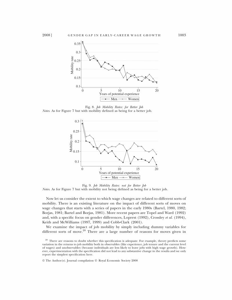
Now let us consider the extent to which wage changes are related to different sorts ofmobility. There is an existing literature on the impact of different sorts of moves onwage changes that starts with a series of papers in the early 1980s (Bartel, 1980, 1982;Borjas, 1981; Bartel and Borjas, 1981). More recent papers are Topel and Ward (1992)and, with a specific focus on gender differences, Loprest (1992), Crossley et al. (1994),Keith and McWilliams (1997, 1999) and Cobb-Clark (2001).We examine the impact of job mobility by simply including dummy variables for
different sorts of move.20 There are a large number of reasons for moves given in
0.1
0.15
0.2
0.25
0.3
0.35
Mob
ility
rat
e
0 5 10 15 20Years of potential experience
Men Women
Fig. 8. Job Mobility Rates: for Better JobNotes. As for Figure 7 but with mobility defined as being for a better job.
0.1
0.15
0.2
0.25
0.3
Mob
ility
rat
e
0 5 10 15 20Years of potential experience
Men Women
Fig. 9. Job Mobility Rates: not for Better JobNotes. As for Figure 7 but with mobility not being defined as being for a better job.
20 There are reasons to doubt whether this specification is adequate. For example, theory predicts somevariation in the returns to job mobility both in observables (like experience, job tenure and the current levelof wages) and unobservables (because individuals are less likely to leave jobs with high wage growth). How-ever, experimentation with the specification did not lead to any substantive change in the results and we onlyreport the simplest specification here.
2008] 1003G E ND E R G A P I N E A R L Y - C A R E E R W AG E G ROWTH
� The Author(s). Journal compilation � Royal Economic Society 2008
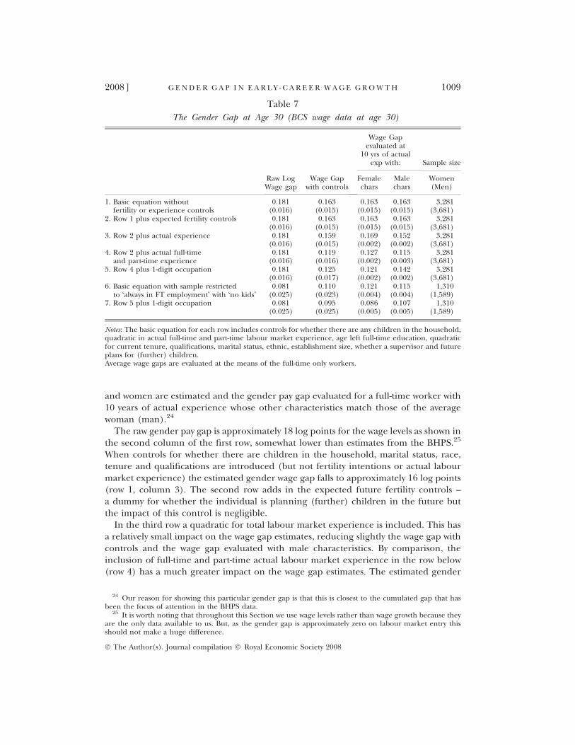
and women are estimated and the gender pay gap evaluated for a full-time worker with10 years of actual experience whose other characteristics match those of the averagewoman (man).24
The raw gender pay gap is approximately 18 log points for the wage levels as shown inthe second column of the first row, somewhat lower than estimates from the BHPS.25
When controls for whether there are children in the household, marital status, race,tenure and qualifications are introduced (but not fertility intentions or actual labourmarket experience) the estimated gender wage gap falls to approximately 16 log points(row 1, column 3). The second row adds in the expected future fertility controls –a dummy for whether the individual is planning (further) children in the future butthe impact of this control is negligible.In the third row a quadratic for total labour market experience is included. This has
a relatively small impact on the wage gap estimates, reducing slightly the wage gap withcontrols and the wage gap evaluated with male characteristics. By comparison, theinclusion of full-time and part-time actual labour market experience in the row below(row 4) has a much greater impact on the wage gap estimates. The estimated gender
Table 7
The Gender Gap at Age 30 (BCS wage data at age 30)
Raw LogWage gap
Wage Gapwith controls
Wage Gapevaluated at
10 yrs of actualexp with: Sample size
Femalechars
Malechars
Women(Men)
1. Basic equation withoutfertility or experience controls
0.181 0.163 0.163 0.163 3,281(0.016) (0.015) (0.015) (0.015) (3,681)
2. Row 1 plus expected fertility controls 0.181 0.163 0.163 0.163 3,281(0.016) (0.015) (0.015) (0.015) (3,681)
3. Row 2 plus actual experience 0.181 0.159 0.169 0.152 3,281(0.016) (0.015) (0.002) (0.002) (3,681)
4. Row 2 plus actual full-timeand part-time experience
0.181 0.119 0.127 0.115 3,281(0.016) (0.016) (0.002) (0.003) (3,681)
5. Row 4 plus 1-digit occupation 0.181 0.125 0.121 0.142 3,281(0.016) (0.017) (0.002) (0.002) (3,681)
6. Basic equation with sample restrictedto �always in FT employment� with �no kids�
0.081 0.110 0.121 0.115 1,310(0.025) (0.023) (0.004) (0.004) (1,589)
7. Row 5 plus 1-digit occupation 0.081 0.095 0.086 0.107 1,310(0.025) (0.025) (0.005) (0.005) (1,589)
Notes: The basic equation for each row includes controls for whether there are any children in the household,quadratic in actual full-time and part-time labour market experience, age left full-time education, quadraticfor current tenure, qualifications, marital status, ethnic, establishment size, whether a supervisor and futureplans for (further) children.Average wage gaps are evaluated at the means of the full-time only workers.
24 Our reason for showing this particular gender gap is that this is closest to the cumulated gap that hasbeen the focus of attention in the BHPS data.
25 It is worth noting that throughout this Section we use wage levels rather than wage growth because theyare the only data available to us. But, as the gender gap is approximately zero on labour market entry thisshould not make a huge difference.
2008] 1009G E ND E R G A P I N E A R L Y - C A R E E R W AG E G ROWTH
� The Author(s). Journal compilation � Royal Economic Society 2008
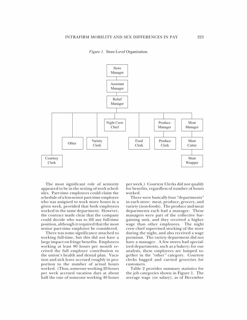
INTRAFIRM MOBILITY AND SEX DIFFERENCES IN PAY 223
The most significant role of seniorityappeared to be in the setting of work sched-ules. Part-time employees could claim theschedule of a less-senior part-time employeewho was assigned to work more hours in agiven week, provided that both employeesworked in the same department. However,the contract made clear that the companycould decide who was to fill any full-timeposition, although it required that the mostsenior part-time employee be considered.
There was some significance attached toworking full-time, but this did not have alarge impact on fringe benefits. Employeesworking at least 80 hours per month re-ceived the full employer contribution tothe union’s health and dental plan. Vaca-tion and sick leave accrued roughly in pro-portion to the number of actual hoursworked. (Thus, someone working 20 hoursper week accrued vacation days at abouthalf the rate of someone working 40 hours
per week.) Courtesy Clerks did not qualifyfor benefits, regardless of number of hoursworked.
There were basically four “departments”in each store: meat, produce, grocery, andvariety (non-foods). The produce and meatdepartments each had a manager. Thesemanagers were part of the collective bar-gaining unit, and they received a higherwage than other employees. The nightcrew chief supervised stocking of the storeduring the night, and also received a wagepremium. The variety department did nothave a manager. A few stores had special-ized departments, such as a bakery; for ouranalysis, these employees are lumped to-gether in the “other” category. Courtesyclerks bagged and carried groceries forcustomers.
Table 2 provides summary statistics forthe job categories shown in Figure 1. Theaverage wage (or salary), as of December
Figure 1. Store-Level Organization.
Store
Manager
Assistant
Manager
Relief
Manager
Meat
Manager
Produce
Manager
Night Crew
Chief
OtherVariety
Clerk
Food
Clerk
Produce
Clerk
Courtesy
Clerk
Meat
Cutter
Meat
Wrapper
226 INDUSTRIAL AND LABOR RELATIONS REVIEW
wage scale as food clerks, but the varietyclerks’ scale was much lower. The averagewage of variety clerks was $1.75 per hourless than that of produce clerks and foodclerks. Courtesy clerks worked for near theminimum wage. There was heavy turnoveramong courtesy clerks, with average senior-ity of only about one year. Courtesy clerkswere about 10 years younger, on average,than food clerks and produce clerks.
Segregation and Wage Differentials
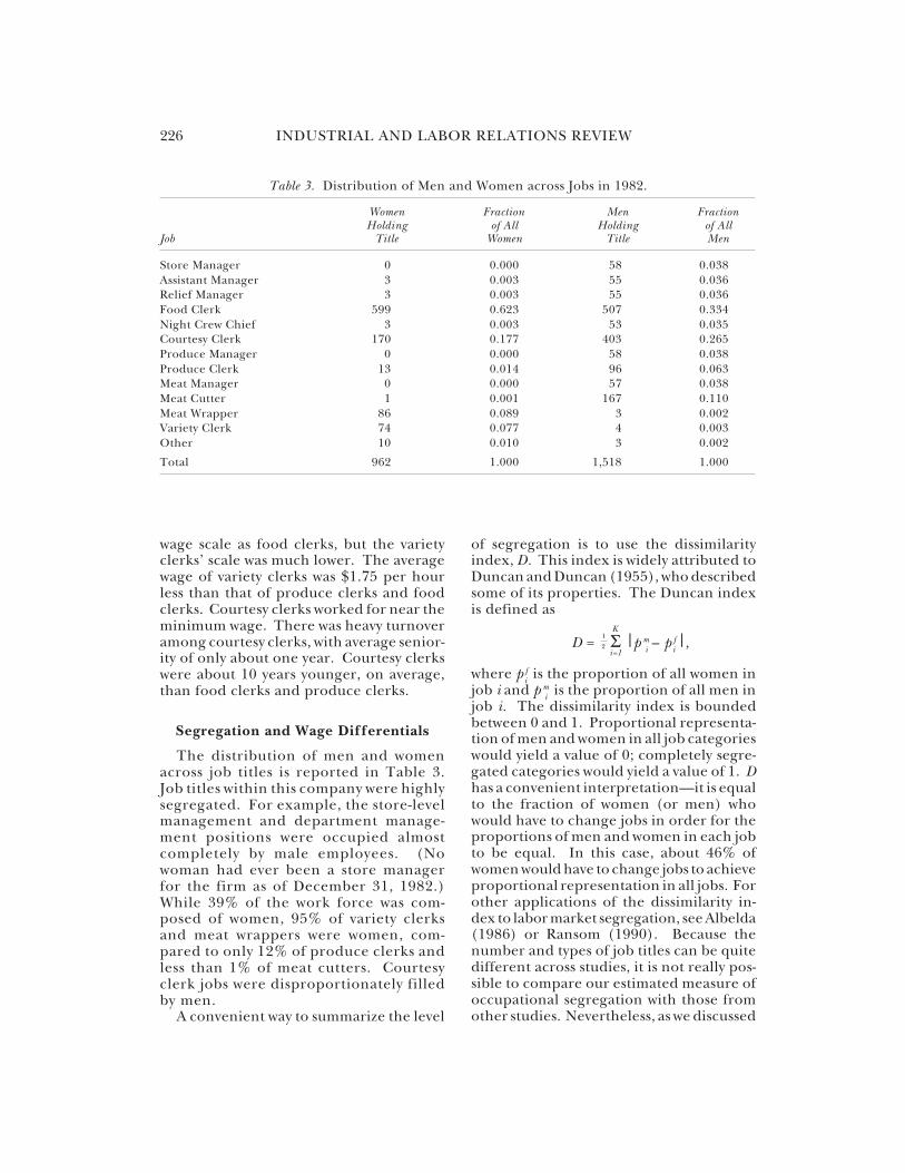
The distribution of men and womenacross job titles is reported in Table 3.Job titles within this company were highlysegregated. For example, the store-levelmanagement and department manage-ment positions were occupied almostcompletely by male employees. (Nowoman had ever been a store managerfor the firm as of December 31, 1982.)While 39% of the work force was com-posed of women, 95% of variety clerksand meat wrappers were women, com-pared to only 12% of produce clerks andless than 1% of meat cutters. Courtesyclerk jobs were disproportionately filledby men.
A convenient way to summarize the level
of segregation is to use the dissimilarityindex, D. This index is widely attributed toDuncan and Duncan (1955), who describedsome of its properties. The Duncan indexis defined as
D = Σ |p mi – p f
i |,
where p fi is the proportion of all women in
job i and p mi is the proportion of all men in
job i. The dissimilarity index is boundedbetween 0 and 1. Proportional representa-tion of men and women in all job categorieswould yield a value of 0; completely segre-gated categories would yield a value of 1. Dhas a convenient interpretation—it is equalto the fraction of women (or men) whowould have to change jobs in order for theproportions of men and women in each jobto be equal. In this case, about 46% ofwomen would have to change jobs to achieveproportional representation in all jobs. Forother applications of the dissimilarity in-dex to labor market segregation, see Albelda(1986) or Ransom (1990). Because thenumber and types of job titles can be quitedifferent across studies, it is not really pos-sible to compare our estimated measure ofoccupational segregation with those fromother studies. Nevertheless, as we discussed
Table 3. Distribution of Men and Women across Jobs in 1982.
Women Fraction Men FractionHolding of All Holding of All
Job Title Women Title Men
Store Manager 0 0.000 58 0.038Assistant Manager 3 0.003 55 0.036Relief Manager 3 0.003 55 0.036Food Clerk 599 0.623 507 0.334Night Crew Chief 3 0.003 53 0.035Courtesy Clerk 170 0.177 403 0.265Produce Manager 0 0.000 58 0.038Produce Clerk 13 0.014 96 0.063Meat Manager 0 0.000 57 0.038Meat Cutter 1 0.001 167 0.110Meat Wrapper 86 0.089 3 0.002Variety Clerk 74 0.077 4 0.003Other 10 0.010 3 0.002
Total 962 1.000 1,518 1.000
K
i=12
1
INTRAFIRM MOBILITY AND SEX DIFFERENCES IN PAY 227
in the introduction, occupational segrega-tion is a well-documented feature of thecontemporary work force.
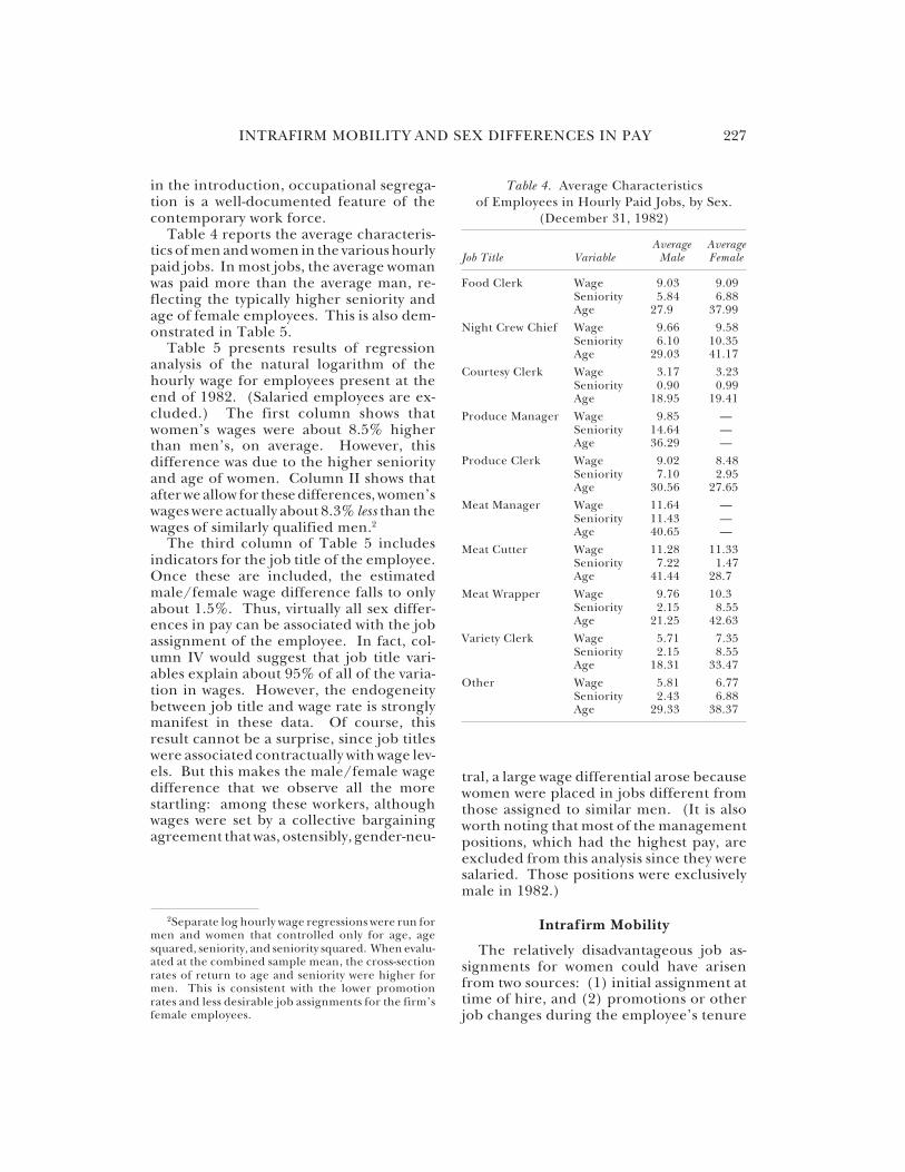
Table 4 reports the average characteris-tics of men and women in the various hourlypaid jobs. In most jobs, the average womanwas paid more than the average man, re-flecting the typically higher seniority andage of female employees. This is also dem-onstrated in Table 5.
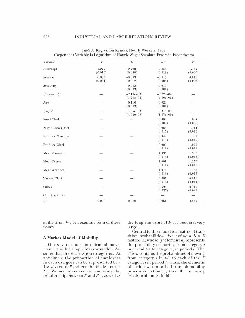
Table 5 presents results of regressionanalysis of the natural logarithm of thehourly wage for employees present at theend of 1982. (Salaried employees are ex-cluded.) The first column shows thatwomen’s wages were about 8.5% higherthan men’s, on average. However, thisdifference was due to the higher seniorityand age of women. Column II shows thatafter we allow for these differences, women’swages were actually about 8.3% less than thewages of similarly qualified men.2
The third column of Table 5 includesindicators for the job title of the employee.Once these are included, the estimatedmale/female wage difference falls to onlyabout 1.5%. Thus, virtually all sex differ-ences in pay can be associated with the jobassignment of the employee. In fact, col-umn IV would suggest that job title vari-ables explain about 95% of all of the varia-tion in wages. However, the endogeneitybetween job title and wage rate is stronglymanifest in these data. Of course, thisresult cannot be a surprise, since job titleswere associated contractually with wage lev-els. But this makes the male/female wagedifference that we observe all the morestartling: among these workers, althoughwages were set by a collective bargainingagreement that was, ostensibly, gender-neu-
tral, a large wage differential arose becausewomen were placed in jobs different fromthose assigned to similar men. (It is alsoworth noting that most of the managementpositions, which had the highest pay, areexcluded from this analysis since they weresalaried. Those positions were exclusivelymale in 1982.)
Intrafirm Mobility
The relatively disadvantageous job as-signments for women could have arisenfrom two sources: (1) initial assignment attime of hire, and (2) promotions or otherjob changes during the employee’s tenure
Table 4. Average Characteristicsof Employees in Hourly Paid Jobs, by Sex.
(December 31, 1982)
Average AverageJob Title Variable Male Female
Food Clerk Wage 9.03 9.09Seniority 5.84 6.88Age 27.9 37.99
Night Crew Chief Wage 9.66 9.58Seniority 6.10 10.35Age 29.03 41.17
Courtesy Clerk Wage 3.17 3.23Seniority 0.90 0.99Age 18.95 19.41
Produce Manager Wage 9.85 —Seniority 14.64 —Age 36.29 —
Produce Clerk Wage 9.02 8.48Seniority 7.10 2.95Age 30.56 27.65
Meat Manager Wage 11.64 —Seniority 11.43 —Age 40.65 —
Meat Cutter Wage 11.28 11.33Seniority 7.22 1.47Age 41.44 28.7
Meat Wrapper Wage 9.76 10.3Seniority 2.15 8.55Age 21.25 42.63
Variety Clerk Wage 5.71 7.35Seniority 2.15 8.55Age 18.31 33.47
Other Wage 5.81 6.77Seniority 2.43 6.88Age 29.33 38.37
2Separate log hourly wage regressions were run formen and women that controlled only for age, agesquared, seniority, and seniority squared. When evalu-ated at the combined sample mean, the cross-sectionrates of return to age and seniority were higher formen. This is consistent with the lower promotionrates and less desirable job assignments for the firm’sfemale employees.
228 INDUSTRIAL AND LABOR RELATIONS REVIEW
Table 5. Regression Results, Hourly Workers, 1982.(Dependent Variable Is Logarithm of Hourly Wage; Standard Errors in Parentheses)
Variable I II III IV
Intercept 1.927 –0.292 0.856 1.152(0.013) (0.048) (0.019) (0.005)
Female 0.085 –0.083 –0.015 0.011(0.021) (0.012) (0.005) (0.005)
Seniority — 0.063 0.019 —(0.003) (0.001)
(Seniority)2 — –2.19e–03 –6.22e–04 —(1.25e–04) (4.60e–05)
Age — 0.116 0.020 —(0.003) (0.001)
(Age)2 — –1.35e–03 –2.31e–04 —(4.02e–05) (1.67e–05)
Food Clerk — — 0.900 1.038(0.007) (0.006)
Night Crew Chief — — 0.963 1.114(0.015) (0.015)
Produce Manager — — 0.942 1.135(0.015) (0.015)
Produce Clerk — — 0.900 1.029(0.011) (0.011)
Meat Manager — — 1.095 1.302(0.016) (0.015)
Meat Cutter — — 1.091 1.270(0.011) (0.010)
Meat Wrapper — — 1.012 1.167(0.013) (0.013)
Variety Clerk — — 0.687 0.811(0.013) (0.014)
Other — — 0.594 0.710(0.027) (0.031)
Courtesy Clerk — — — —
R2 0.008 0.680 0.961 0.949
at the firm. We will examine both of theseissues.
A Markov Model of Mobility
One way to capture intrafirm job move-ments is with a simple Markov model. As-sume that there are K job categories. Atany time t, the proportion of employeesin each category can be represented by a1 × K vector, Pt , where the i th element isPit . We are interested in examining therelationship between Pt and Pt–1, as well as
the long-run value of Pt as t becomes verylarge.
Central to this model is a matrix of tran-sition probabilities. We define a K × Kmatrix, A, whose ijth element aij representsthe probability of moving from category iin period t–1 to category j in period t. Theith row contains the probabilities of movingfrom category i in t–1 to each of the Kcategories in period t. Thus, the elementsof each row sum to 1. If the job mobilityprocess is stationary, then the followingrelationship must hold:
INTRAFIRM MOBILITY AND SEX DIFFERENCES IN PAY 235
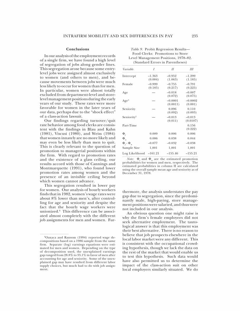
Table 9. Probit Regression Results—Food Clerks: Promotions to Store
Level Management Positions, 1978–82.(Standard Errors in Parentheses)
Variable I II III
Intercept –1.363 –0.952 –1.299(0.084) (1.063) (1.185)
Female –0.999 –0.755 –0.791(0.185) (0.217) (0.225)
Age — –0.018 –0.007(0.072) (0.075)
Age2 — –0.0001 –0.0002(0.0011) (0.001)
Seniority — 0.096 0.110(0.092) (0.093)
Seniority2 — –0.013 –0.013(0.011) (0.0107)
Part-Time 0.156(0.222)
Φf 0.009 0.006 0.006
Φm 0.086 0.038 0.044
Φf - Φm –0.077 –0.032 –0.038
Sample Size 1,001 1,001 1,001
Log Likelihood –161.21 –155.46 –155.21
Note: Φf and Φm are the estimated promotionprobabilities for women and men, respectively. Theestimated probabilities in column II are calculatedusing the overall sample mean age and seniority as ofDecember 31, 1978.
Conclusions
In our analysis of the employment recordsof a single firm, we have found a high levelof segregation of jobs along gender lines.This segregation arose because some entry-level jobs were assigned almost exclusivelyto women (and others to men), and be-cause movements between jobs were muchless likely to occur for women than for men.In particular, women were almost totallyexcluded from department-level and store-level management positions during the earlyyears of our study. These rates were morefavorable for women in the later years ofour data, perhaps due to the “shock effect”of a class-action lawsuit.
Our findings regarding turnover/quitrate behavior among food clerks are consis-tent with the findings in Blau and Kahn(1981), Viscusi (1980), and Weiss (1984)that women innately are no more likely andmay even be less likely than men to quit.This is clearly relevant to the question ofpromotion to managerial positions withinthe firm. With regard to promotion ratesand the existence of a glass ceiling, ourresults accord with those of Cannings andMontmarquette (1991), who found lowerpromotion rates among women and thepresence of an invisible ceiling beyondwhich women cannot advance.
This segregation resulted in lower payfor women. Our analysis of hourly workersfinds that in 1982, women’s wage rates wereabout 8% lower than men’s, after control-ling for age and seniority and despite thefact that the hourly wage workers wereunionized.6 This difference can be associ-ated almost completely with the differentjob assignments for men and women. Fur-
6Oaxaca and Ransom (1994) reported wage de-compositions based on a 1986 sample from the samefirm. Separate (log) earnings equations were esti-mated for men and women. Depending on the typeof decomposition used, the unexplained earningsgap ranged from 28.8% to 33.1% in favor of men afteraccounting for age and seniority. Some of the unex-plained gap may have resulted from different laborsupply choices, but much had to do with job assign-ment.
thermore, the analysis understates the paygap due to segregation, since the predomi-nantly male, high-paying, store manage-ment positions were salaried, and thus werenot included in our analysis.
An obvious question one might raise iswhy the firm’s female employees did notseek alternative employment. The tauto-logical answer is that this employment wastheir best alternative. There is no reason tobelieve that job prospects elsewhere in thelocal labor market were any different. Thisis consistent with the occupational crowd-ing hypothesis, though we lack the data onthe rest of the market that would enable usto test this hypothesis. Such data wouldhave also permitted us to determine theimpact of the class-action suit on otherlocal employers similarly situated. We do
This content downloaded from 128.32.105.184 on Fri, 18 Nov 2016 07:25:26 UTCAll use subject to http://about.jstor.org/terms
27
Tables
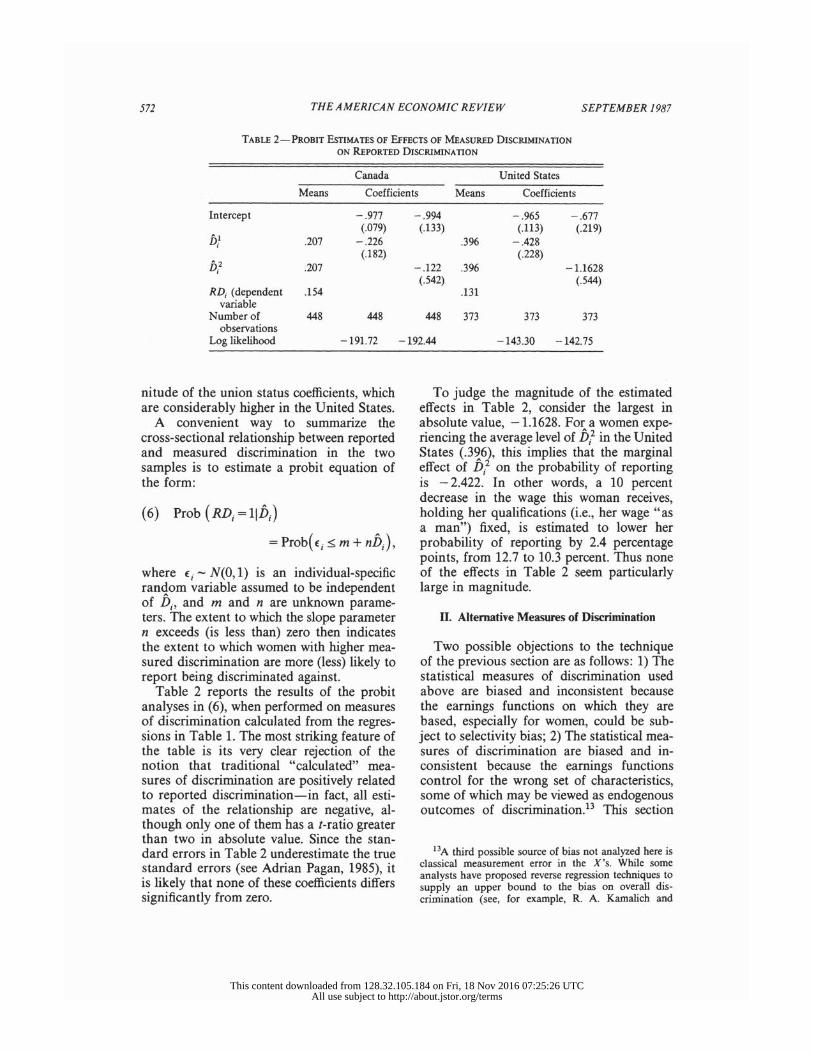
TABLE 1 SUMMARY STATISTICS ON WAGE BIDS AND WAGE OFFERS
BMALE‡ BFEM‡
Raw-Wage gap
PWMALE‡ PWFEM‡ Raw-Wage gap
WAGE BID (SEK) 19 312*** 18 196 0.942 (3 288.5) (2 663.9) ln. WAGE BID 9.85*** 9.80 WAGE OFFER (SEK) 18 628***a 17 517 a 0.938 16 925*** 16 047 0.948 (3 311.1) (2560.2) (2 964.1) (2 337.6) ln. WAGE OFFER 9.82*** 9.76 9.72*** 9.67 No of Obs 901 1222 812 1030 Note: Numbers in parentheses are standard deviations. ‡ “B” refers to those choosing a job involving individual wage bargaining and “PW” refers to those choosing a job with a posted wage. ***/**/* denote statistical gender differences at the 1/5/10 percent levels respectively in a t-test of equal variance. a/b/c denote statistical difference between bargainers and non-bargainers at the 1/5/10 percent levels respectively.
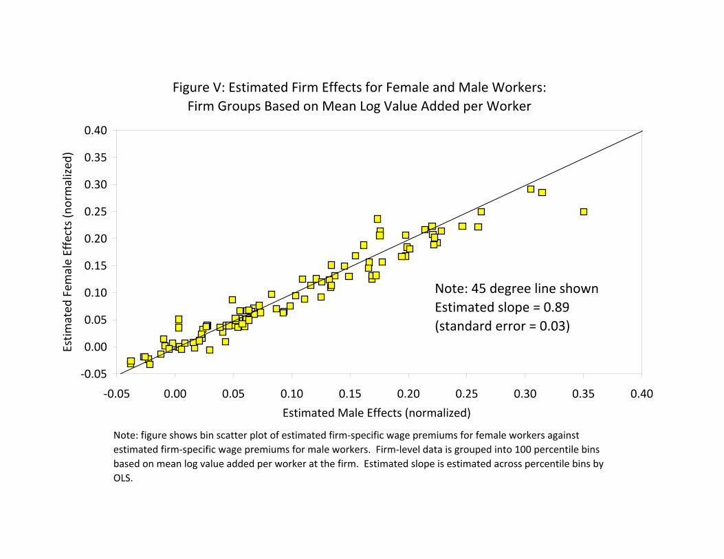
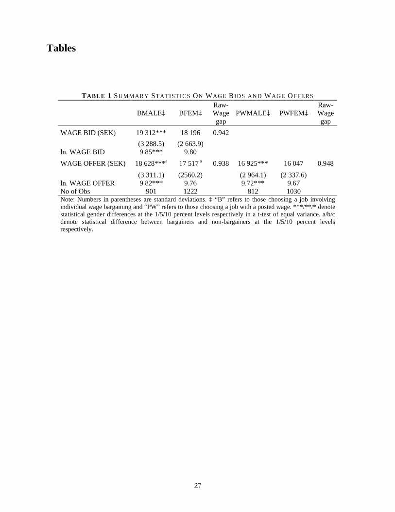
Figure V: Estimated Firm Effects for Female and Male Workers: Firm Groups Based on Mean Log Value Added per Worker
‐0.05
0.00
0.05
0.10
0.15
0.20
0.25
0.30
0.35
0.40
‐0.05 0.00 0.05 0.10 0.15 0.20 0.25 0.30 0.35 0.40Estimated Male Effects (normalized)
Estim
ated
Fem
ale Effects (no
rmalize
d)
Note: 45 degree line shownEstimated slope = 0.89(standard error = 0.03)
Note: figure shows bin scatter plot of estimated firm‐specific wage premiums for female workers against estimated firm‐specific wage premiums for male workers. Firm‐level data is grouped into 100 percentile bins based on mean log value added per worker at the firm. Estimated slope is estimated across percentile bins by OLS.
Table III: Contribution of Firm‐Specific Pay Premiums to the Gender Wage Gap at Dual Connected Firms
Male Prem. Female Prem. Using M Using F Using M Using FAmong Men Among Women Effects Effects Distribution Distribution
(1) (2) (3) (4) (5) (6) (7) (8)
All 0.234 0.148 0.099 0.049 0.035 0.047 0.003 0.015(21.2) (14.9) (19.9) (1.2) (6.3)
By Age Group:Up to age 30 0.099 0.114 0.087 0.028 0.019 0.029 ‐0.001 0.009
(28.2) (18.9) (29.3) 1.2 (9.3)
Ages 31‐40 0.228 0.156 0.111 0.045 0.029 0.040 0.004 0.016(19.7) (12.6) (17.8) (1.9) (7.0)
Over Age 40 0.336 0.169 0.099 0.069 0.050 0.064 0.005 0.019(20.6) (15.0) (19.1) (1.5) (5.6)
By Education Group:< High School 0.286 0.115 0.055 0.059 0.045 0.061 ‐0.002 0.015
(20.8) (15.6) (21.4) (0.6) (5.2)
High School 0.262 0.198 0.137 0.061 0.051 0.051 0.010 0.010(23.3) (19.6) (19.5) (3.8) (3.7)
University 0.291 0.259 0.213 0.047 0.025 0.029 0.018 0.022(16.1) (8.7) (9.9) (6.2) (7.4)
Notes: Sample includes male and female workers in "dual connected" set (Table I, columns 5‐6). Entry in column 1 is the difference in mean log wages of males and females, estimated over all workers in the subset of the dual connected set indicated by the row heading. Estimated firm effects are from models described in columns 1 and 2 of Table II. Entry in column 4 is the total contribution of firm‐specific wage premiums to the gender wage gap reported in column 1. Entries in columns 5‐8 are the contributions of sorting effect and bargaining effect to gender wage gap. Entries in parentheses represent the percent of the overall male female wage gap (in column 1) that is explained by the source described in column heading.
Total Contribution of
Firm Components
Decompositions of Contribution of Firm ComponentSorting BargainingMeans of Firm Premiums:
Gender Wage Gap
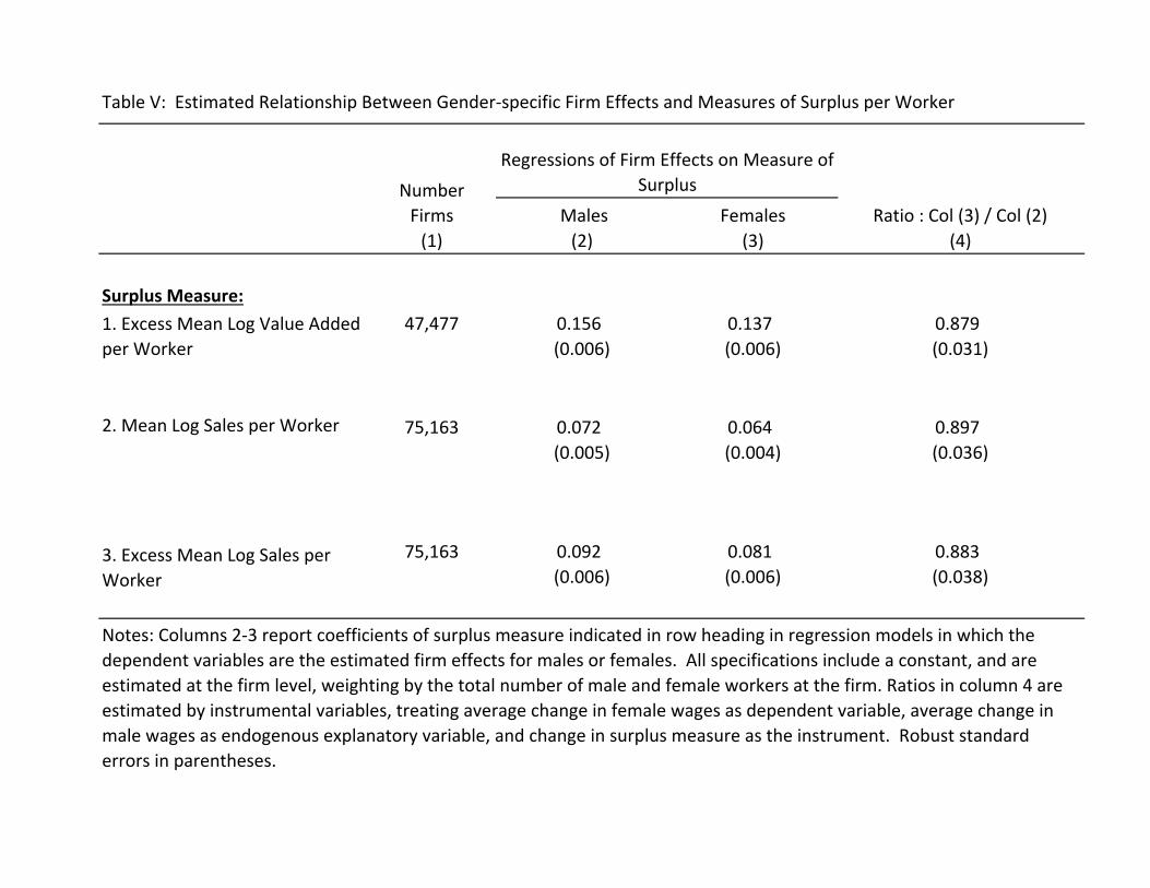
Table V: Estimated Relationship Between Gender‐specific Firm Effects and Measures of Surplus per Worker
Males Females(1) (2) (3) (4)
Surplus Measure:47,477 0.156 0.137 0.879
(0.006) (0.006) (0.031)
75,163 0.072 0.064 0.897(0.005) (0.004) (0.036)
75,163 0.092 0.081 0.883(0.006) (0.006) (0.038)
Regressions of Firm Effects on Measure of SurplusNumber
Firms Ratio : Col (3) / Col (2)
2. Mean Log Sales per Worker
3. Excess Mean Log Sales per Worker
Notes: Columns 2‐3 report coefficients of surplus measure indicated in row heading in regression models in which the dependent variables are the estimated firm effects for males or females. All specifications include a constant, and are estimated at the firm level, weighting by the total number of male and female workers at the firm. Ratios in column 4 are estimated by instrumental variables, treating average change in female wages as dependent variable, average change in male wages as endogenous explanatory variable, and change in surplus measure as the instrument. Robust standard errors in parentheses.
1. Excess Mean Log Value Added per Worker
234 AMERICAN ECONOMIC JOURNAL: APPLIED ECONOMICS JULY 2010
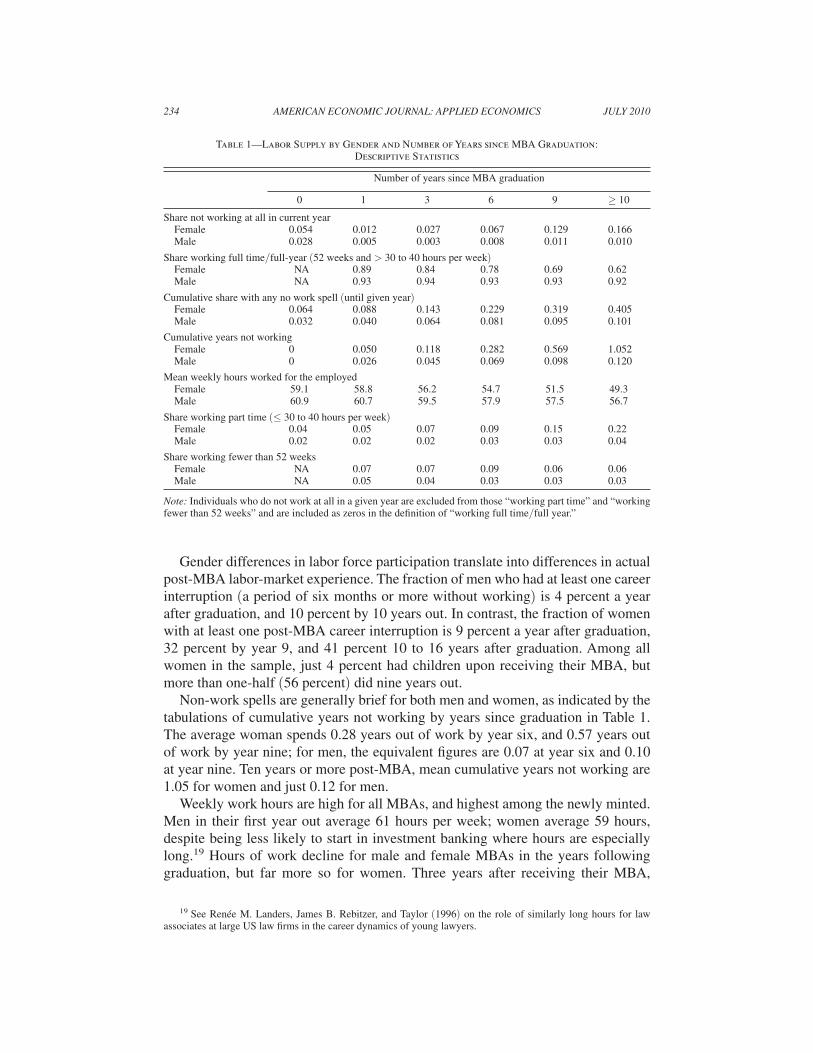
Gender differences in labor force participation translate into differences in actual post-MBA labor-market experience. The fraction of men who had at least one career interruption (a period of six months or more without working) is 4 percent a year after graduation, and 10 percent by 10 years out. In contrast, the fraction of women with at least one post-MBA career interruption is 9 percent a year after graduation, 32 percent by year 9, and 41 percent 10 to 16 years after graduation. Among all women in the sample, just 4 percent had children upon receiving their MBA, but more than one-half (56 percent) did nine years out.
Non-work spells are generally brief for both men and women, as indicated by the tabulations of cumulative years not working by years since graduation in Table 1. The average woman spends 0.28 years out of work by year six, and 0.57 years out of work by year nine; for men, the equivalent figures are 0.07 at year six and 0.10 at year nine. Ten years or more post-MBA, mean cumulative years not working are 1.05 for women and just 0.12 for men.
Weekly work hours are high for all MBAs, and highest among the newly minted. Men in their first year out average 61 hours per week; women average 59 hours, despite being less likely to start in investment banking where hours are especially long.19 Hours of work decline for male and female MBAs in the years following graduation, but far more so for women. Three years after receiving their MBA,
19 See Renée M. Landers, James B. Rebitzer, and Taylor (1996) on the role of similarly long hours for law associates at large US law firms in the career dynamics of young lawyers.
Table 1—Labor Supply by Gender and Number of Years since MBA Graduation: Descriptive Statistics
Number of years since MBA graduation
0 1 3 6 9 ≥ 10
Share not working at all in current year Female 0.054 0.012 0.027 0.067 0.129 0.166 Male 0.028 0.005 0.003 0.008 0.011 0.010
Share working full time/full-year (52 weeks and > 30 to 40 hours per week) Female NA 0.89 0.84 0.78 0.69 0.62 Male NA 0.93 0.94 0.93 0.93 0.92
Cumulative share with any no work spell (until given year) Female 0.064 0.088 0.143 0.229 0.319 0.405 Male 0.032 0.040 0.064 0.081 0.095 0.101
Cumulative years not working Female 0 0.050 0.118 0.282 0.569 1.052 Male 0 0.026 0.045 0.069 0.098 0.120
Mean weekly hours worked for the employed Female 59.1 58.8 56.2 54.7 51.5 49.3 Male 60.9 60.7 59.5 57.9 57.5 56.7
Share working part time (≤ 30 to 40 hours per week) Female 0.04 0.05 0.07 0.09 0.15 0.22 Male 0.02 0.02 0.02 0.03 0.03 0.04
Share working fewer than 52 weeks Female NA 0.07 0.07 0.09 0.06 0.06 Male NA 0.05 0.04 0.03 0.03 0.03
Note: Individuals who do not work at all in a given year are excluded from those “working part time” and “working fewer than 52 weeks” and are included as zeros in the definition of “working full time/full year.”
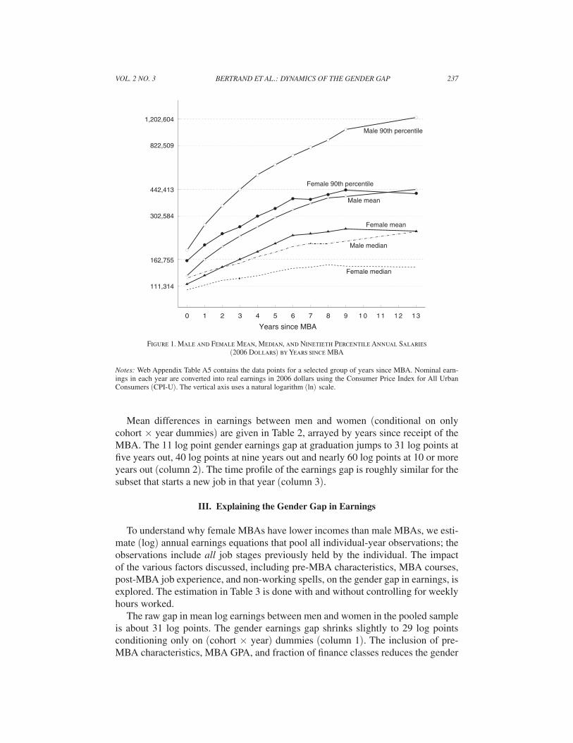
VOL. 2 NO. 3 237BERTRAND ET AL.: DYNAMICS OF THE GENDER GAP
Mean differences in earnings between men and women (conditional on only cohort × year dummies) are given in Table 2, arrayed by years since receipt of the MBA. The 11 log point gender earnings gap at graduation jumps to 31 log points at five years out, 40 log points at nine years out and nearly 60 log points at 10 or more years out (column 2). The time profile of the earnings gap is roughly similar for the subset that starts a new job in that year (column 3).
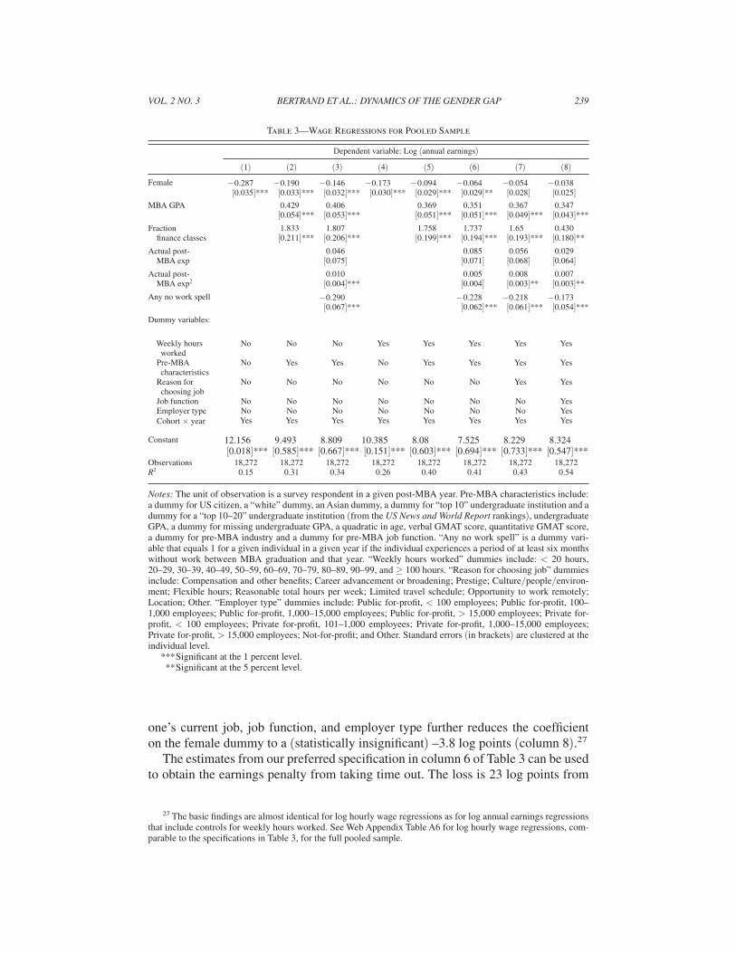
III. Explaining the Gender Gap in Earnings
To understand why female MBAs have lower incomes than male MBAs, we esti-mate (log) annual earnings equations that pool all individual-year observations; the observations include all job stages previously held by the individual. The impact of the various factors discussed, including pre-MBA characteristics, MBA courses, post-MBA job experience, and non-working spells, on the gender gap in earnings, is explored. The estimation in Table 3 is done with and without controlling for weekly hours worked.
The raw gap in mean log earnings between men and women in the pooled sample is about 31 log points. The gender earnings gap shrinks slightly to 29 log points conditioning only on (cohort × year) dummies (column 1). The inclusion of pre-MBA characteristics, MBA GPA, and fraction of finance classes reduces the gender
0 1 2 3 4 5 6 7 8 9 1 0 1 1 1 2 1 3
Years since MBA
162,755
442,413
1,202,604
111,314
302,584
822,509
Male mean
Female mean
Male 90th percentile
Male median
Female 90th percentile
Female median
Figure 1. Male and Female Mean, Median, and Ninetieth Percentile Annual Salaries (2006 Dollars) by Years since MBA
Notes: Web Appendix Table A5 contains the data points for a selected group of years since MBA. Nominal earn-ings in each year are converted into real earnings in 2006 dollars using the Consumer Price Index for All Urban Consumers (CPI-U). The vertical axis uses a natural logarithm (ln) scale.
VOL. 2 NO. 3 239BERTRAND ET AL.: DYNAMICS OF THE GENDER GAP
one’s current job, job function, and employer type further reduces the coefficient on the female dummy to a (statistically insignificant) –3.8 log points (column 8).27
The estimates from our preferred specification in column 6 of Table 3 can be used to obtain the earnings penalty from taking time out. The loss is 23 log points from
27 The basic findings are almost identical for log hourly wage regressions as for log annual earnings regressions that include controls for weekly hours worked. See Web Appendix Table A6 for log hourly wage regressions, com-parable to the specifications in Table 3, for the full pooled sample.
Table 3—Wage Regressions for Pooled Sample
Dependent variable: Log (annual earnings)
(1) (2) (3) (4) (5) (6) (7) (8)
Female − 0.287[0.035]***
− 0.190[0.033]***
− 0.146[0.032]***
− 0.173[0.030]***
− 0.094[0.029]***
− 0.064[0.029]**
− 0.054[0.028]
− 0.038[0.025]
MBA GPA 0.429[0.054]***
0.406[0.053]***
0.369[0.051]***
0.351[0.051]***
0.367[0.049]***
0.347[0.043]***
Fraction finance classes
1.833[0.211]***
1.807[0.206]***
1.758[0.199]***
1.737[0.194]***
1.65[0.193]***
0.430[0.180]**
Actual post- MBA exp
0.046[0.075]
0.085[0.071]
0.056[0.068]
0.029[0.064]
Actual post- MBA exp2
0.010[0.004]***
0.005[0.004]
0.008[0.003]**
0.007[0.003]**
Any no work spell − 0.290[0.067]***
− 0.228[0.062]***
− 0.218[0.061]***
− 0.173[0.054]***
Dummy variables:
Weekly hours worked
No No No Yes Yes Yes Yes Yes
Pre-MBA characteristics
No Yes Yes No Yes Yes Yes Yes
Reason for choosing job
No No No No No No Yes Yes
Job function No No No No No No No Yes Employer type No No No No No No No Yes Cohort × year Yes Yes Yes Yes Yes Yes Yes Yes
Constant 12.156[0.018]***
9.493[0.585]***
8.809[0.667]***
10.385[0.151]***
8.08[0.603]***
7.525[0.694]***
8.229[0.733]***
8.324[0.547]***
Observations 18,272 18,272 18,272 18,272 18,272 18,272 18,272 18,272R2 0.15 0.31 0.34 0.26 0.40 0.41 0.43 0.54
Notes: The unit of observation is a survey respondent in a given post-MBA year. Pre-MBA characteristics include: a dummy for US citizen, a “white” dummy, an Asian dummy, a dummy for “top 10” undergraduate institution and a dummy for a “top 10–20” undergraduate institution (from the US News and World Report rankings), undergraduate GPA, a dummy for missing undergraduate GPA, a quadratic in age, verbal GMAT score, quantitative GMAT score, a dummy for pre-MBA industry and a dummy for pre-MBA job function. “Any no work spell” is a dummy vari-able that equals 1 for a given individual in a given year if the individual experiences a period of at least six months without work between MBA graduation and that year. “Weekly hours worked” dummies include: < 20 hours, 20–29, 30–39, 40–49, 50–59, 60–69, 70–79, 80–89, 90–99, and ≥ 100 hours. “Reason for choosing job” dummies include: Compensation and other benefits; Career advancement or broadening; Prestige; Culture/people/environ-ment; Flexible hours; Reasonable total hours per week; Limited travel schedule; Opportunity to work remotely; Location; Other. “Employer type” dummies include: Public for-profit, < 100 employees; Public for-profit, 100–1,000 employees; Public for-profit, 1,000–15,000 employees; Public for-profit, > 15,000 employees; Private for-profit, < 100 employees; Private for-profit, 101–1,000 employees; Private for-profit, 1,000–15,000 employees; Private for-profit, > 15,000 employees; Not-for-profit; and Other. Standard errors (in brackets) are clustered at the individual level.
*** Significant at the 1 percent level. ** Significant at the 5 percent level.
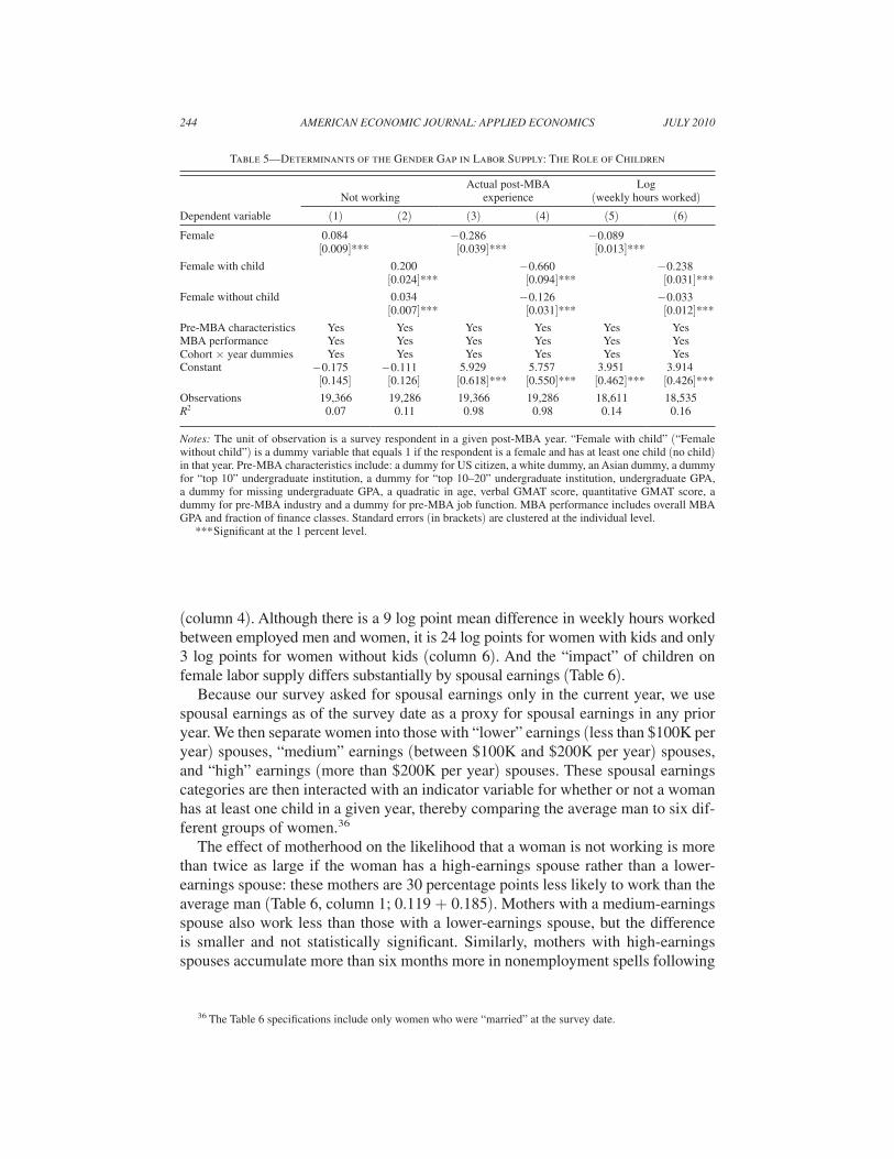
244 AMERICAN ECONOMIC JOURNAL: APPLIED ECONOMICS JULY 2010
(column 4). Although there is a 9 log point mean difference in weekly hours worked between employed men and women, it is 24 log points for women with kids and only 3 log points for women without kids (column 6). And the “impact” of children on female labor supply differs substantially by spousal earnings (Table 6).
Because our survey asked for spousal earnings only in the current year, we use spousal earnings as of the survey date as a proxy for spousal earnings in any prior year. We then separate women into those with “lower” earnings (less than $100K per year) spouses, “medium” earnings (between $100K and $200K per year) spouses, and “high” earnings (more than $200K per year) spouses. These spousal earnings categories are then interacted with an indicator variable for whether or not a woman has at least one child in a given year, thereby comparing the average man to six dif-ferent groups of women.36
The effect of motherhood on the likelihood that a woman is not working is more than twice as large if the woman has a high-earnings spouse rather than a lower-earnings spouse: these mothers are 30 percentage points less likely to work than the average man (Table 6, column 1; 0.119 + 0.185). Mothers with a medium-earnings spouse also work less than those with a lower-earnings spouse, but the difference is smaller and not statistically significant. Similarly, mothers with high-earnings spouses accumulate more than six months more in nonemployment spells following
36 The Table 6 specifications include only women who were “married” at the survey date.
Table 5—Determinants of the Gender Gap in Labor Supply: The Role of Children
Not working
Actual post-MBA experience
Log (weekly hours worked)
Dependent variable (1) (2) (3) (4) (5) (6)
Female 0.084 − 0.286 − 0.089[0.009]*** [0.039]*** [0.013]***
Female with child 0.200 − 0.660 − 0.238[0.024]*** [0.094]*** [0.031]***
Female without child 0.034 − 0.126 − 0.033[0.007]*** [0.031]*** [0.012]***
Pre-MBA characteristics Yes Yes Yes Yes Yes YesMBA performance Yes Yes Yes Yes Yes YesCohort × year dummies Yes Yes Yes Yes Yes YesConstant − 0.175 − 0.111 5.929 5.757 3.951 3.914
[0.145] [0.126] [0.618]*** [0.550]*** [0.462]*** [0.426]***
Observations 19,366 19,286 19,366 19,286 18,611 18,535R2 0.07 0.11 0.98 0.98 0.14 0.16
Notes: The unit of observation is a survey respondent in a given post-MBA year. “Female with child” (“Female without child”) is a dummy variable that equals 1 if the respondent is a female and has at least one child (no child) in that year. Pre-MBA characteristics include: a dummy for US citizen, a white dummy, an Asian dummy, a dummy for “top 10” undergraduate institution, a dummy for “top 10–20” undergraduate institution, undergraduate GPA, a dummy for missing undergraduate GPA, a quadratic in age, verbal GMAT score, quantitative GMAT score, a dummy for pre-MBA industry and a dummy for pre-MBA job function. MBA performance includes overall MBA GPA and fraction of finance classes. Standard errors (in brackets) are clustered at the individual level.
*** Significant at the 1 percent level.
248 AMERICAN ECONOMIC JOURNAL: APPLIED ECONOMICS JULY 2010
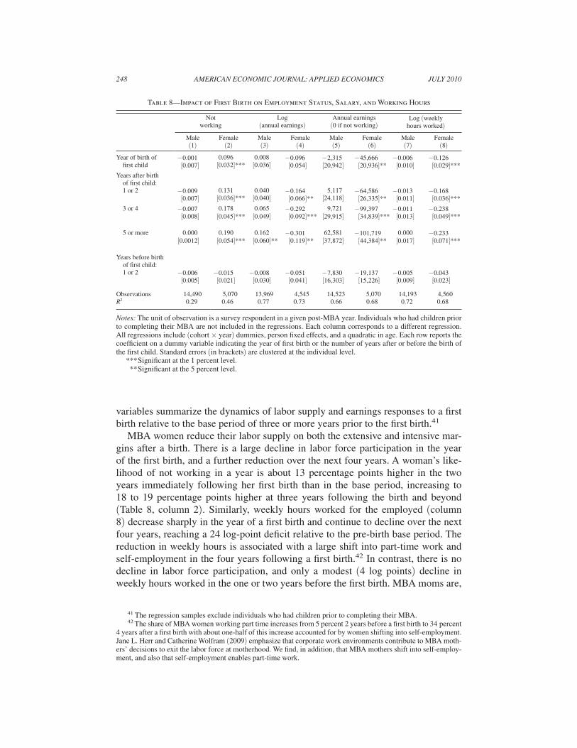
variables summarize the dynamics of labor supply and earnings responses to a first birth relative to the base period of three or more years prior to the first birth.41
MBA women reduce their labor supply on both the extensive and intensive mar-gins after a birth. There is a large decline in labor force participation in the year of the first birth, and a further reduction over the next four years. A woman’s like-lihood of not working in a year is about 13 percentage points higher in the two years immediately following her first birth than in the base period, increasing to 18 to 19 percentage points higher at three years following the birth and beyond (Table 8, column 2). Similarly, weekly hours worked for the employed (column 8) decrease sharply in the year of a first birth and continue to decline over the next four years, reaching a 24 log-point deficit relative to the pre-birth base period. The reduction in weekly hours is associated with a large shift into part-time work and self-employment in the four years following a first birth.42 In contrast, there is no decline in labor force participation, and only a modest (4 log points) decline in weekly hours worked in the one or two years before the first birth. MBA moms are,
41 The regression samples exclude individuals who had children prior to completing their MBA.42 The share of MBA women working part time increases from 5 percent 2 years before a first birth to 34 percent
4 years after a first birth with about one-half of this increase accounted for by women shifting into self-employment. Jane L. Herr and Catherine Wolfram (2009) emphasize that corporate work environments contribute to MBA moth-ers’ decisions to exit the labor force at motherhood. We find, in addition, that MBA mothers shift into self-employ-ment, and also that self-employment enables part-time work.
Table 8—Impact of First Birth on Employment Status, Salary, and Working Hours
Not working
Log (annual earnings)
Annual earnings(0 if not working)
Log (weekly hours worked)
Male(1)
Female(2)
Male(3)
Female(4)
Male(5)
Female(6)
Male(7)
Female(8)
Year of birth of first child
− 0.001[0.007]
0.096[0.032]***
0.008[0.036]
− 0.096[0.054]
− 2,315[20,942]
− 45,666[20,936]**
− 0.006[0.010]
− 0.126[0.029]***
Years after birth of first child: 1 or 2 − 0.009
[0.007]0.131[0.036]***
0.040[0.040]
− 0.164[0.066]**
5,117[24,118]
− 64,586[26,335]**
− 0.013[0.011]
− 0.168[0.036]***
3 or 4 − 0.007 0.178 0.065 − 0.292 9,721 − 99,397 − 0.011 − 0.238[0.008] [0.045]*** [0.049] [0.092]*** [29,915] [34,839]*** [0.013] [0.049]***
5 or more 0.000 0.190 0.162 − 0.301 62,581 − 101,719 0.000 − 0.233[0.0012] [0.054]*** [0.060]** [0.119]** [37,872] [44,384]** [0.017] [0.071]***
Years before birth of first child: 1 or 2 − 0.006 − 0.015 − 0.008 − 0.051 − 7,830 − 19,137 − 0.005 − 0.043
[0.005] [0.021] [0.030] [0.041] [16,303] [15,226] [0.009] [0.023]
Observations 14,490 5,070 13,969 4,545 14,523 5,070 14,193 4,560R2 0.29 0.46 0.77 0.73 0.66 0.68 0.72 0.68
Notes: The unit of observation is a survey respondent in a given post-MBA year. Individuals who had children prior to completing their MBA are not included in the regressions. Each column corresponds to a different regression. All regressions include (cohort × year) dummies, person fixed effects, and a quadratic in age. Each row reports the coefficient on a dummy variable indicating the year of first birth or the number of years after or before the birth of the first child. Standard errors (in brackets) are clustered at the individual level.
*** Significant at the 1 percent level. ** Significant at the 5 percent level.
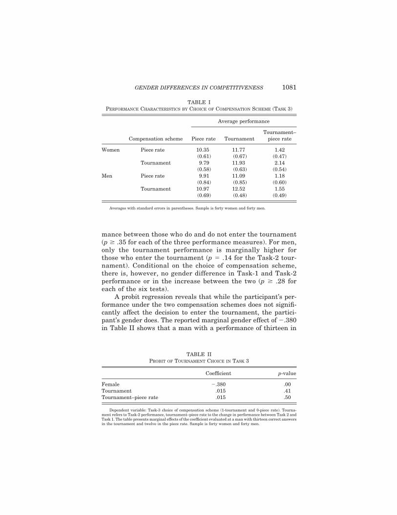
mance between those who do and do not enter the tournament(p � .35 for each of the three performance measures). For men,only the tournament performance is marginally higher forthose who enter the tournament (p � .14 for the Task-2 tour-nament). Conditional on the choice of compensation scheme,there is, however, no gender difference in Task-1 and Task-2performance or in the increase between the two (p � .28 foreach of the six tests).
A probit regression reveals that while the participant’s per-formance under the two compensation schemes does not signifi-cantly affect the decision to enter the tournament, the partici-pant’s gender does. The reported marginal gender effect of �.380in Table II shows that a man with a performance of thirteen in
TABLE IPERFORMANCE CHARACTERISTICS BY CHOICE OF COMPENSATION SCHEME (TASK 3)
Compensation scheme
Average performance
Piece rate TournamentTournament–
piece rate
Women Piece rate 10.35 11.77 1.42(0.61) (0.67) (0.47)
Tournament 9.79 11.93 2.14(0.58) (0.63) (0.54)
Men Piece rate 9.91 11.09 1.18(0.84) (0.85) (0.60)
Tournament 10.97 12.52 1.55(0.69) (0.48) (0.49)
Averages with standard errors in parentheses. Sample is forty women and forty men.
TABLE IIPROBIT OF TOURNAMENT CHOICE IN TASK 3
Coefficient p-value
Female �.380 .00Tournament .015 .41Tournament–piece rate .015 .50
Dependent variable: Task-3 choice of compensation scheme (1-tournament and 0-piece rate). Tourna-ment refers to Task-2 performance, tournament–piece rate to the change in performance between Task 2 andTask 1. The table presents marginal effects of the coefficient evaluated at a man with thirteen correct answersin the tournament and twelve in the piece rate. Sample is forty women and forty men.
1081GENDER DIFFERENCES IN COMPETITIVENESS


