1362 IEEE TRANSACTIONS ON AUTOMATIC...

1362 IEEE TRANSACTIONS ON AUTOMATIC CONTROL, VOL. 52, NO. 8, AUGUST 2007

Trajectory-Tracking and Path-Following ofUnderactuated Autonomous Vehicles With

Parametric Modeling UncertaintyA. Pedro Aguiar, Member, IEEE, and João P. Hespanha, Senior Member, IEEE

Abstract—We address the problem of position trajec-tory-tracking and path-following control design for underactuatedautonomous vehicles in the presence of possibly large modelingparametric uncertainty. For a general class of vehicles moving ineither 2- or 3-D space, we demonstrate how adaptive switchingsupervisory control can be combined with a nonlinear Lya-punov-based tracking control law to solve the problem of globalboundedness and convergence of the position tracking error to aneighborhood of the origin that can be made arbitrarily small.The desired trajectory does not need to be of a particular type(e.g., trimming trajectories) and can be any sufficiently smoothbounded curve parameterized by time. We also show how theseresults can be applied to solve the path-following problem, inwhich the vehicle is required to converge to and follow a path,without a specific temporal specification. We illustrate our designprocedures through two vehicle control applications: a hovercraft(moving on a planar surface) and an underwater vehicle (movingin 3-D space). Simulations results are presented and discussed.

Index Terms—Path-following, supervisory adaptive control, tra-jectory-tracking, underactuated autonomous vehicles.

I. INTRODUCTION

THE past few decades have witnessed an increased researcheffort in the area of motion control of autonomous vehi-

cles. A typical motion control problem is trajectory-tracking,which is concerned with the design of control laws that force avehicle to reach and follow a time parameterized reference (i.e.,a geometric path with an associated timing law). The degree ofdifficulty involved in solving this problem is highly dependenton the configuration of the vehicle. For fully actuated systems,the trajectory-tracking problem is now reasonably well under-stood.

Manuscript received June 30, 2005; revised May 8, 2006. Recommended byAssociate Editor A. Garulli. This work was supported in part by the NationalScience Foundation under Grant ECS-0093762, Project MAYA-Sub of the AdI(PT), project GREX/CEC-IST under Contract 035223, of the Commission of theEuropean Communities, and by the FCT-ISR/IST plurianual funding throughthe POS_C Program that includes FEDER funds.

A. P. Aguiar was with the Center for Control Engineering and Computation,University of California, Santa Barbara, CA 93106 USA. He is now with theInstitute for Systems and Robotics, Instituto Superior Técnico, Lisbon, Portugal(e-mail: [email protected]).

J. P. Hespanha is with the Center for Control Engineering and Computa-tion, University of California, Santa Barbara, CA 93106 USA (e-mail: [email protected]).

Color versions of one or more of the figures in this paper available online athttp://ieeexplore.ieee.org.

Digital Object Identifier 10.1109/TAC.2007.902731

For underactuated vehicles, i.e., systems with fewer actua-tors than degrees-of-freedom,1 trajectory-tracking is still an ac-tive research topic. The study of these systems is motivated bythe fact that it is usually costly and often not practical to fullyactuate autonomous vehicles due to weight, reliability, com-plexity, and efficiency considerations. Typical examples of un-deractuated systems include wheeled robots, hovercraft, space-craft, aircraft, helicopters, missiles, surface vessels, and under-water vehicles. The tracking problem for underactuated vehi-cles is especially challenging because most of these systems arenot fully feedback linearizable and exhibit nonholonomic con-straints. The reader is refereed to [3] for a survey of these con-cepts and to [4] for a framework to study the controllability andthe design of motion algorithms for underactuated Lagrangiansystems on Lie groups.

The classical approach for trajectory-tracking of underactu-ated vehicles utilizes local linearization and decoupling of themulti-variable model to steer the same number of degrees offreedom as the number of available control inputs, which canbe done using standard linear (or nonlinear) control methods.Alternative approaches include the linearization of the vehicleerror dynamics around trajectories that lead to a time-invariantlinear system (also known as trimming trajectories) combinedwith gain scheduling and/or linear parameter varying (LPV) de-sign methodologies [5]–[7]. The basic limitation of these ap-proaches is that stability is only guaranteed in a neighborhood ofthe selected operating points. Moreover, performance can suffersignificantly when the vehicle executes maneuvers that empha-size its nonlinearity and cross couplings. A different approachis to use output feedback linearization methods, [8]–[10]. Themajor challenge in this approach is that a straightforward appli-cation of this methodology, which in general involves dynamicinversion, is not always possible because certain involutivityconditions must hold [11]. In addition, even when dynamic in-version is possible, the resulting controller may not render thezero-dynamics stable.

Nonlinear Lyapunov-based designs can overcome some ofthe limitations mentioned above. Several examples of nonlinear

1The following definition of underactuated mechanical systems is adaptedfrom [1], [2]. Consider the affine mechanical system described by

�q = f(q; _q) +G(q)u (1)

where q is a vector of independent generalized coordinates, f a vector field thatcaptures the dynamics of the system, G the input matrix, and u the vector ofgeneralized inputs. Equation (1) is underactuated if the rank ofG is smaller thanthe dimension of q, i.e., the generalized inputs are not able to instantaneouslyset the accelerations in all directions of the configuration space.

0018-9286/$25.00 © 2007 IEEE

AGUIAR AND HESPANHA: UNDERACTUATED AUTONOMOUS VEHICLES 1363

trajectory-tracking controllers for marine underactuated vehi-cles have been reported in the literature [12]–[19]. Typically,tracking problems for autonomous vehicles are solved by de-signing control laws that make the vehicles track pre-specifiedfeasible “state-space” trajectories, i.e., trajectories that specifythe time evolution of the position, orientation, as well as thelinear and angular velocities, all consistent with the vehicles’dynamics, [8], [13], [15]–[20], even through in practical appli-cations one often only needs to track a desired position. Thisapproach suffers from the drawback that usually the vehicles’dynamics exhibit complex nonlinear terms and significant un-certainty, which makes the task of computing a feasible trajec-tory difficult.

It is relevant to point out that most of the results mentionedabove only solve the problem in the horizontal plane. Only a fewauthors have tackled this control problems in 3-D space. Thereason might be that the vehicle’s dynamics become more com-plex and the number of degree of freedom that are not directlyactuated typically increases, making the control design more in-volved. For example, for an underactuated underwater vehicle,the dynamics include sway and heave velocities that generatenonzero angles of sideslip and attack.

Motivated by these considerations, we propose a solution tothe trajectory-tracking problem for underactuated vehicles inboth 2- and 3-D spaces. In this paper, we are especially inter-ested in situations for which there is parametric uncertainty inthe model of the vehicle. Typical parameters for which this un-certainty is high, include mass and added mass for underwatervehicles which may be subject to large variations accordingto the payload configuration, and friction coefficients that areusually strongly dependent on the environmental conditions.The main contribution of the paper is the design of an adap-tive supervisory control algorithm that combines logic-basedswitching [21] with iterative Lyapunov-based techniques suchas integrator backstepping [22]. The classical approach to adap-tive control relies solely on continuous tuning [22]–[24]. Thisapproach has some inherent limitations that can be overcome byhybrid adaptive algorithms based on switching and logic [25].The basic idea behind supervisory control [21], [26]–[30] is todesign a suitable family of candidate controllers. Each controlleris designed for an admissible nominal model of the process, anda supervision logic orchestrates the switching among the can-didate controllers, deciding, at each instant of time, the can-didate feedback controller that is more adequate. In order toguarantee stability and avoid chattering, a form of hysteresisis employed. We prove that the adaptive controller solves theproblem of global boundedness and convergence of the positiontracking error to a neighborhood of the origin that can be madearbitrarily small in the presence of possible large parametric un-certainty. The adaptive supervisory controller does not requirepersistence of excitation which sets it apart from most param-eter estimation algorithms. In the control design, we take intoaccount that the vehicle may have non-negligible dynamics andmay undergo complex motions and exhibit large angles of attackand sideslip, which prevents us from using simple extensions ofcommon control designs for wheeled robots where the total ve-locity vector is aligned with the vehicles main axis. Also, thedesired trajectory does not need to be a trimming trajectory and

can be any sufficiently smooth time-varying bounded curve, in-cluding the degenerate case of a constant trajectory (set-point).The class of vehicles for which the design procedure is ap-plicable is quite general and includes any vehicle modeled asa rigid-body subject to a controlled force and either one con-trolled torque if it is only moving on a planar surface or twoor three independent control torques for a vehicle moving in3-D space. Furthermore, contrary to most of the approaches de-scribed above, the controller proposed does not suffer from geo-metric singularities due to the parameterization of the vehicle’srotation matrix. This is possible because the attitude controlproblem is formulated directly in the group of rotations .The literature on designing tracking control laws for underac-tuated vehicles directly in the configuration manifold (avoidingin this way geometric singularities) is relatively scarce. Note-worthy examples include [20] and [31].

Another contribution of this paper is the application of theseresults to solve the path-following motion control problem. Inpath-following, the vehicle is required to converge to and followa path that is specified without a temporal law [32]–[36]. Pi-oneering work in this area for wheeled mobile robots is de-scribed in [32]. In [34], Samson addressed the path-followingproblem for a car pulling several trailers. More recently, Altafini[36] describes a path-following controller for a trailer ve-hicle that provides local asymptotic stability for a path of non-constant curvature. Path-following controllers for aircraft andmarine vehicles have been reported in [6], [9], and [37]–[39].Using the approach suggested by Hauser and Hindman [37], anoutput maneuvering controller was proposed in [39] for a classof strict feedback nonlinear processes and applied to path-fol-lowing of fully actuated ships. The underlying assumption inpath-following is that the vehicle’s forward speed tracks a de-sired speed profile, while the controller acts on the vehicle’sorientation to drive it to the path. Typically, in path-following,smoother convergence to the path is achieved and the controlsignals are less likely pushed into saturation, when compared totrajectory-tracking. In fact, in [40] and [41], we highlight a fun-damental difference between path-following and standard tra-jectory-tracking by demonstrating that performance limitationsdue to unstable zero-dynamics can be removed in the path-fol-lowing problem. Inspired by these ideas, we solve the path-fol-lowing problem by decomposing it into two subproblems: i) ageometric task, which consists of converging the vehicle to andremaining inside a tube centered around the desired path, andii) a dynamic assignment task, which assigns a speed profile tothe path.

In Section II, we describe the dynamic model for the classof underactuated autonomous vehicles considered in the paperand formulate the trajectory-tracking and path-following controlproblems. As a preliminary material for the subsequent sections,Section III presents a nonlinear control law to solve the trackingproblem and discusses the stability of the resulting closed-loop.At this point it is assumed that there is no parametric uncertainty.Sections IV and V present the main results of the paper. In Sec-tion IV, a solution to the trajectory-tracking is proposed usingan estimator-based supervisory controller, and in Section V anextension is made to solve the path-following problem. In Sec-tion VI, we illustrate our design methodologies in the context


of two vehicle control applications: a hovercraft (moving ona planar surface) and an underwater vehicle (moving in 3-Dspace). The designs are validated through computer simulations.The paper concludes with a summary of the results and sugges-tions for further research.

A subset of the results reported here were presented in[42]–[44].

Notation: Throughout this paper, given a matrix , de-notes its transpose, , are the minimum andmaximum eigenvalues of , respectively. Given two vectors

, , we denote by the vector. The Euclidean norm is denoted by

and the spectral norm by . A piecewise continuous func-tion , is in , being a positiveinteger, if for some constant .

II. PROBLEM STATEMENT

Consider an underactuated vehicle modeled as a rigid bodysubject to external forces and torques. Let be an inertial co-ordinate frame and a body-fixed coordinate frame whoseorigin is located at the center of mass of the vehicle. The con-figuration of the vehicle is an element of the Special Eu-clidean group , where

is a rotation matrixthat describes the orientation of the vehicle by mapping bodycoordinates into inertial coordinates, and is the positionof the origin of in . Denoting by and thelinear and angular velocities of the vehicle relative to ex-pressed in , respectively, the following kinematic relationsapply:

(2a)

(2b)

where is a function from to the space of skew-symmetricmatrices defined by

We consider here underactuated vehicles with dynamic equa-tions of motion of the following form:

(3a)

(3b)

where and denote constant symmetricpositive definite mass and inertia matrices; anddenote the control inputs, which act upon the system through aconstant nonzero vector and a constant nonsingular ma-trix2 , respectively; the terms in (3a) and

in (3b) are the rigid-body Coriolis terms,and the functions , represent all the remaining

2See Remark 4 for the special case of G 2 .

forces and torques acting on the body. For the special case ofan underwater vehicle, and also include the so-called hy-drodynamic added-mass and added-inertia matrices, re-spectively, i.e., , , whereand are the rigid-body mass and inertia matrices, respec-tively.

For an underactuated vehicle restricted to moving on a planarsurface, the same equations of motion (2), (3) apply withoutthe first two right-hand side terms in (3b). Also, in this case,

, , , , ,, with all the other terms in (3) having appropriate

dimensions, and the skew-symmetric matrix is given by

. For simplicity, in what follows, we re-

strict our attention to the 3-D case. However, all results are di-rectly applicable to the 2-D case, as will be illustrated in Sec-tion VI-A for the control of a Hovercraft.

Remark 1: The vehicle dynamic model (3) does not allowto depend on . This was done in part to simplify the anal-

ysis and also because in many vehicles this dependance is notpresent as is the case of the Hovercraft and the AUV described inSection VI. The methodology presented here still applies for themore general case if the dependence on is in the form

, provided that is bounded orthat a suitable rank condition holds. For details see Property 1in the Appendix and [42], [44].

The problems considered in this paper can be stated as fol-lows:

Trajectory-tracking problem: Letbe a given sufficiently smooth time-varying desired trajec-tory with its time-derivatives bounded. Design a controllersuch that all the closed-loop signals are bounded and thetracking error converges to a neighborhoodof the origin that can be made arbitrarily small.Path-following problem: Let be a desiredpath parameterized by and a desiredspeed3 assignment. Suppose also that is sufficientlysmooth with respect to and its derivatives (with respect to

) are bounded. Design feedback control laws for , ,and such that all the closed-loop signals are bounded,the position of the vehicle converges to and remains in-side a tube centered around the desired path that can bemade arbitrarily thin, i.e., converges toa neighborhood of the origin that can be made arbitrarilysmall, and the vehicle satisfies a desired speed assignment

along the path, i.e., the speed error canbe confined to an arbitrarily small ball.

III. TRAJECTORY-TRACKING CONTROLLER DESIGN

A. Controller Design

This section proposes a Lyapunov-based control law to solvethe trajectory-tracking problem assuming that there is no para-metric uncertainty. For the sake of clarity, control-Lyapunovfunctions are introduced iteratively borrowing from the tech-niques of backstepping [22].

3For simplicity of presentation it will be assumed that the speed assignmentv ( ) 2 does not depend directly on time t.


Step 1. Coordinate transformation: Consider the global dif-feomorphic coordinate transformation

which expresses the tracking error in the body-fixedframe. The dynamic equation of the body-fixed trackingerror is given by

Step 2. Convergence of : We start by defining the control-Lyapunov function

and computing its time derivative to obtain

(4)

We can regard as a virtual control that one would useto make negative. This could be achieved, by settingequal to , for some positive constant .To accomplish this we introduce the error variable

that we would like to drive to zero, and re-write (4) as

(5)

Step 3. Backstepping for : After straightforward alge-braic manipulations, the dynamic equation of the errorcan be written as

where

(6)

and. It turns out that it will not always be pos-

sible to drive to zero. We need to explore the couplingof the translation dynamics with the rotational inputs. Tothis effect, we will drive to a constant design vector

. To achieve this we define as a newerror variable that we will drive to zero and consider theaugmented control-Lyapunov function

The time derivative of can be written as

(7)

where

(8)

In Appendix (cf. Property 1), we show that the matrix Bcan always be made full-rank by choosing a suitable .One can now regard as a virtual control (actually its firstcomponent is already a “real” control) that one would liketo use to make negative. This could be achieved, bysetting equal to

where is a symmetric positive definite matrix.To accomplish this we set to be equal to the first entryof , i.e.,

(9)

and introduce the error variable

that one would like to set to zero. We can now rewrite (7),with given by (9), as

Step 4. Backstepping for : Consider now a third control-Lyapunov function given by

(10)

Computing its time derivative one obtains

For simplicity, we did not expand the derivative of . If wethen choose

(11)


where is a symmetric positive matrix, the timederivative of becomes

Note that although is not necessarily always negative,this will be sufficient to prove boundedness and conver-gence of to a neighborhood of the origin.

B. Stability Analysis

We can now prove that all signals will remain bounded, andthat the tracking error converges exponential to an arbitrarilysmall neighborhood of the origin.

Theorem 1: Given a sufficiently smooth time-varying desiredtrajectory with its time-derivatives bounded,consider the nonlinear system described by the underactuatedvehicle model (2), (3) in closed-loop with the feedback con-troller (9), (11).

(i) For every initial condition of , the solution exists glob-ally, all closed-loop signals are bounded, and the trackingerror satisfies

(12)

where , , and are positive constants. From these, onlydepends on initial conditions.

(ii) For a given upper bound on , by appropriatechoice of the controller parameters , anydesired values for and in (12) are possible.

Proof: To prove (i) we use Young’s inequality4 to concludethat for any

(13)Suppose now that we choose sufficiently small so that thematrix is positive definite. In this case weconclude that there is a sufficiently small positive constantsuch that

(14)

and, therefore, it is straightforward to conclude from the Com-parison Lemma [45] that

(15)

along solutions to . From here we conclude that all signals re-main bounded and therefore the solution exists globally. More-over, converges to a ball of radius and therefore

converges to a ball of radius , because of (10).To prove (ii), we show next that the radius can be

made as small as we want by appropriately choosing the con-

4A special case of the Young’s inequality is ab � ( =2)a + (1=2 )b ,where a; b � 0, and is any positive constant.

troller parameters. To this effect, suppose we pick a desired ra-dius and a convergence rate , and we select such that Bis full rank. Such value for may depend on the upper bound of

(see Property 1). We can then define ,provided that we choose sufficiently large so that

If we then select , , we con-clude from (13) that (14) indeed holds for the prespecified ,from which (15) follows. However, now the above choices forthe parameters lead to a radius .

Remark 2: We did not impose any constraints on the desiredtrajectory (besides being sufficiently smooth and its derivativebeing bounded) and we also did not require that the linear ve-locity of the vehicle be always nonnull. Consequently, canbe arbitrary, that is, the desired trajectories do not need to sat-isfy “dynamic” models, and in particular can be constant for all

. In that case, the controller solves the position regulationproblem.

Remark 3: In practice, the vector determines if the vehiclewill follow the desired trajectory backward or forward. To ob-serve this, define the following two angles:and , where , , and are thethree components of the body-fixed tracking error . Notice that

and can be seen as the elevation and azimuth angles, respec-tively. In steady-state (with , ), from (5), it followsthat . Thus, when the first com-ponent of is negative and larger (in absolute value) thanthe other two components, the vehicle will converge to the tra-jectory with positive surge velocity, and will stay “behind” thedesired trajectory, see examples in Section VI.

Remark 4: When the vehicle is subject to one controlled forceand only two independent control torques, i.e., , but

(and consequently ), one can use, e.g.,, provided that there exists a

symmetric positive definite matrix such that(which is the case for the AUV in Section VI). If we then set

the time derivative of becomes

where is a disturbance term that depends on the componentof the state in the null space of . From the above, onecan prove boundedness if this component is bounded. For un-derwater vehicles, this component typically corresponds to theroll motion which usually is stable due to the restoring forces.

IV. ESTIMATOR-BASED SUPERVISORY CONTROL

Using the previous results, this section proposes an es-timator-based supervisory control architecture to solve the


Fig. 1. Supervisory control architecture.

trajectory-tracking problem in the presence of parametric mod-eling uncertainty. Let be a vector that contains allthe unknown parameters of the dynamic equations of motion(3), where denotes the number of unknown parameters. Thefollowing technical assumption is assumed to hold.

Assumption 1: Let be a finite set of candidate parametervalues

The actual parameter belongs to .In practice, this assumption can be relaxed to being

sufficiently close to an element of , which can be achievedby taking a fine grid, at the price of increased computationalburden.

The supervisory consists of three subsystems (see Fig. 1)[21].

multi-estimator—a dynamical system whose inputs are theprocess input and its output , and whose outputs are ,

, where each is a suitably defined estimate ofwhich would be asymptotically correct if was equal to

.multi-controller—a dynamical system whose inputs are theoutput estimate and the estimation errors ,

, and whose outputs are the control signals ,, where each is generated by a control law that

would be adequate if was equal to .switching logic—a dynamical system whose inputs are theestimation errors and whose output is a switching signal

which is used to define the control law .

The underlying decision-making strategy used by theswitching logic basically consists of selecting for , thecandidate controller index for which the correspondingperformance signal (which is a suitably “normed” valueof ) is currently the smallest. This strategy is motivatedby the idea that the nominal process model with the smallestperformance signal is the one that “best” approximates theactual process, and, thus, the candidate controller associatedwith that model can be expected to have a better performanceof controlling the process.

In this paper we assume that the whole state of the processis available for feedback. Therefore,

, and . Since thereis no uncertainty in (2), we can simply pick and

. We also restrict our attention to state feedback laws and,therefore, .

A. Multi-Estimator

This section addresses the design of a family of estimatorsparameterized by for the underactuated vehicle model(2), (3). Motivated by Assumption 1 and in view of (3), we con-sider a family of estimators of the form5

(16a)

(16b)

where , are diagonal positive definitematrices and for each the scalar positive func-tions and

satisfy6

(17a)

(17b)

(17c)

for some positive constants , . The functionsand will be defined later (cf. (28a), (28b)). The

multi-estimator has the desirable property that the estimatorerror that corresponds to the actual parameter value con-verges exponentially to zero and satisfies a -like property.

Lemma 1: Let be the actual parameter value. Thereexist , , such that for every initial condition of(2), (3), (16), and continuous signal , there existpositive constants , , that depend on the initial conditionssuch that

(18a)

(18b)

(18c)

5WhenP has a large number of elements, an alternative approach is describedin Section IV-E.

6The existence of � (�) and � (�) follows directly from the fact thatf (�) and f (�) are C .


for every time in the maximum interval of existence of solutionto the closed-loop , .

Proof: See the Appendix.

B. Multi-Controller

We now design a family of candidate feedback lawssuch that for each , wouldsolve the tracking problem formulated in Section II for a processmodel given by (2) and (16), and “sufficiently” small estima-tion errors , . For a given , we design by con-structing control-Lyapunov functions iteratively, following thedesign procedure proposed in Section III.

Step 1 and 2: Same as in Section III. However, in this caseis redefined as

(19)

and, therefore

Step 3: The dynamic equation of the error is now givenby

where

Thus, is redefined as

where . The time derivative of can bewritten as

where

(20)

Following the same line of reason described in Step 3 ofSection III, let

(21)be a virtual control law for each , where is chosensuch that is nonsingular. Let be equal to the firstentry of , i.e.

(22)

and

(23)

Then

Step 4: The third control-Lyapunov function is now givenby

(24)

Computing its time derivative one obtains

where can be decomposed in two terms:. Here, , and is defined to be the


same as , but substituting the arguments , by , ,respectively. Selecting

(25)

where for each , is a symmetricpositive matrix, the time derivative of becomes

(26)

where

(27)

The last term can be rewritten as, where

(28a)

(28b)

From (26), although has indefinite terms, it will be ver-ified that they will be dominated by the negative definiteterms when the estimator errors , are sufficientlysmall. This is stated in the following lemma.

Lemma 2: Let , denote the maximum in-terval of existence of solution to the closed-loop and supposethat there exists a time such that for all

and

(29)

where the control law is defined in (22) and (25) and

(30)

Given a sufficiently smooth time-varying desired trajectorywith its time-derivatives bounded and any initial

condition of the resulting closed-loop system, the signals ,, , and are bounded on . Moreover, if

(29) holds with , then, as , the tracking errorconverges to a neighborhood of the origin that can

be made arbitrarily small by appropriate choice of the controllerparameters.

Proof: See the Appendix.Loosely speaking, Lemma 2 states that each candidate con-

troller solves the trajectory-tracking problem formulated in Sec-tion II provided that the input disturbances due to the estimationerrors have finite energy as defined by the integral (29). Theswitching-logic will guarantee that (29) holds by the Scale-In-dependent Hysteresis Switching Lemma [21] (cf. proof of The-orem 2).

C. Switching-Logic

Motivated by (29), (30), for each , we start by definingthe performance signal as the state of the dynamic equation

(31)

with the initial values satisfying . Equation (31)implies that each performance signal is the sum of an expo-nentially decaying term that depends on initial conditions anda suitable exponentially weighted “norm” of the correspondingestimation errors. The control parameter acts as a forgettingfactor in the evaluation of the performance signals, henceestablishing a compromise between adaptation alertness andswitching dither.

The switching logic consider here is the scale-independenthysteresis switching logic proposed in [21]. Let be a posi-tive constant called the hysteresis constant. The operation of theswitching logic can be briefly explained as follows: First, we set

. Suppose that at a certain timethe value of has just switched to some . Then, willbe kept fixed until a time such that

at which point we set to .When the indicated minimum is not unique, a particular valuefor among those that achieve the minimum can be chosen ar-bitrarily. Repeating this procedure, a piecewise constant signal

is generated that is continuous from right everywhere. Set-ting for all avoids chattering. The switchingsignal is used to define the control signal as follows:

(32)

where the candidate control laws are defined by (22) and(25).


D. Stability Analysis

We are now ready to prove that all closed-loop signals willremain bounded, and that the tracking error converges to an ar-bitrarily small neighborhood of the origin in the presence of pos-sible large parametric modeling uncertainty.

Theorem 2: Given a sufficiently smooth time-varying de-sired trajectory with its time-derivativesbounded, consider the hybrid system described by theunderactuated vehicle model (2), (3) in closed-loop with theswitched multi-controller (32), the multi-estimator (16), and theswitching logic described in Section IV-C.

i) For any initial condition of with ,, the solution exists globally and all closed-loop signals

are bounded.ii) Furthermore, there exists a finite time such that

for all (i.e., the switchingstops in finite time) and as the tracking error

converges to a neighborhood of the originthat can be made arbitrarily small by appropriate choiceof the control parameters.

Proof: Consider the scaled performance signals, . From (31) we conclude that

(33)

Because of the scale independence property of the switchinglogic, replacing by would have no effect on . From(33) we see that each is nondecreasing. This, the finitenessof , and the fact that for each guarantee theexistence of a positive number such that , ,

. It is not hard to conclude from the definition of theswitching logic that chattering cannot occur. In fact, there mustbe an interval of maximal length on which the solutionof the system is defined, and can only have a finite number ofdiscontinuities on each proper subinterval of . For details,see [21]. To prove that the switching stops in finite time, observefrom (33) and (30) that is bounded by virtue of Lemma1. It follows now that the signals satisfy the hypotheses ofthe Scale-Independent Hysteresis Switching Lemma [21] whichenables us to conclude that the switching stops in finite time.More precisely, there exists a time such that

for all . In addition, is bounded on. Using (33) with and the boundedness of ,

we see that the integral

is finite (recall that is positive). Therefore, resorting toLemma 2, this implies that , , , and are bounded on

.

Next we will prove that and are also bounded on, where is the actual parameter value. Consider

the following nonnegative function

(34)

Its time derivative satisfies (c.f. Appendix)

(35)

where , , are functions in defined on, and , are functions in defined on. Consider now the ordinary differential equation

(36)

Using [46, Lemma 1]] we conclude that for any initial condi-tion, the solution to (36) exists and is bounded on .Moreover, when , converges to as .Thus, applying the Comparison Lemma to (35) it can be con-cluded that and, consequently, , are bounded on

. Since is bounded by virtue of Lemma 1, it followsthat is bounded on . Com-bining the boundedness of and with the estimators(16), it can be seen that the dynamic equations for the quadraticestimation error , can be expressed (after ap-plying the Comparison Lemma) as an exponential stable linearsystem with bounded inputs. Therefore, this implies that and

are bounded on for each. Since all signals are bounded in the maximal interval

of existence of solutions, one conclude that the solutions existglobally, i.e., . The convergence of the tracking error

to a neighborhood of the origin now follows fromLemma 2.

E. State-Sharing

In the previous sections, we have relied on the fact that theset was finite, so that the estimators (16). If the set isinfinite or it has a large number of elements, a different ap-proach is required. One alternative, which leads to a more ef-ficient design, is to replace the individual estimator equationsby a single system and use it to generate the estimation errors.In other words, to make the estimators in (16) “share” the samestate. The performance signals can be obtained in a similarway. To this effect, suppose that the functions , and

are separable on the unknown parameter , i.e,take the form . In that case, we can define


and replace the estimators (16) by

(37a)

(37b)

(37c)

(37d)

with outputs

where

Note that and satisfy (16) but with possible largerand that still satisfy (17). However, the dimension of (37)is now independent of the number of elements in .

V. PATH-FOLLOWING CONTROLLER DESIGN

In this section, inspired by [39], the results described in Sec-tion IV are utilized to solve the path-following problem. Let

be a desired geometric path parameterized by a vari-able and a desired speed assignment. Contraryto trajectory-tracking, in path-following we have the freedom toselect a timing law for . In particular, we can regardas an additional control input. In this paper, we actually regard

as the additional input, because this will necessarily pro-duce a differentiable . Let us define the position body-fixedpath-following error

and the speed error . Following the same stepsdescribed in Section III and IV-B, and defining [see (19)]as

where , we obtain

Notice also that

where

and , . Therefore, using(21)–(23), we obtain

where

Notice that can be decomposed as .Thus, if we then choose

(38)

the time derivative of becomes


where , , is defined to be the sameas , but substituting , by , , and

Introduce now a forth control Lyapunov function given by

Computing its time derivative, we get

Selecting the following update law for :

(39)where is a positive constant, we obtain

An extension of Theorem 2 to the path-following then follows.Theorem 3: Given a sufficiently smooth (with respect to )

desired path with its derivatives (with respectto ) bounded, and a desired assignment speed ,consider the hybrid system described by the underactu-ated vehicle model (2), (3) in closed-loop with the switchedmulti-controller (22), (38), (39), the multi-estimator (16), andthe switching logic described in Section IV-C.

i) For any initial condition of with ,, the solution exists globally and all closed-loop signals

are bounded.ii) There exist a finite time such that

for all (i.e., the switching stops in finite time).Moreover, as , the position errorand the speed error converge to neigh-borhoods of the origin that can be made arbitrarily smallby appropriate choice of the control parameters.

Proof: The proof is not given since it is a simple applicationof the arguments used in the previous theorems.

VI. APPLICATION TO SPECIFIC VEHICLES

This section illustrates the application of the previous resultsto two vehicles: a hovercraft (moving on a planar surface) andan underwater vehicle (moving in 3-D space).

A. Trajectory-Tracking of an Underactuated Hovercraft

Consider the Caltech MVWT vehicle described in [43], [47]consisting of a platform mounted on three low-friction, omni-directional casters, with two attached high-performance ductedfans. Let be the Cartesian coordinates of thevehicle’s center of mass and its orientation. Assumingthat the friction and moment forces can be modeled by viscousfriction, the equations of motion are

where is the mass of the vehicle andis the rotational inertia. The starboard

and portboard fan forces are denoted and , respectively,and denotes the moment arm of the forces.The geometric and mass centers of the vehicle are assumedto coincide. The coefficient of viscous friction is 5.5Kg/s and the coefficient of rotational friction is 0.41 Kgm/s. Expressing the equations of motion in the body fixedframe, yields (2) and (3) with , ,

, , ,

, , ,, , , , and

. In this case the matrix B introduced in (8) is

given by with . The reader is

referred to [43] for a detailed coverage of the trajectory-trackingcontroller with experimental results.

We now describe two simulation results that illustrate the per-formance of the proposed tracking controller with and withoutsupervisory control. The objective of the first experiment is toforce the hovercraft to track the “virtual” kinematic unicycle ve-hicle

which starts at and moves withvelocities and . The initialconditions for the hovercraft are ,

, . For simplicity, only the coefficientof viscous friction is unknown, but assumed to belong to theset . The control parameters wereselected as follows: , , , and

for all . The hysteresis constant forthe switching logic was set to , the forgetting factorto , and the multi-estimator gains to and

. The functions and introduced in (16) aregiven by .

To illustrate the benefits derived from the supervisory con-trol scheme proposed in Section IV, we show in Fig. 2(a) theclosed-loop trajectory for the (nonadaptive) trajectory-trackingcontroller presented in Section III when the value of the coef-ficient of viscous friction assumed by the control system wasset to 10% of the real value. It can be seen that although the


Fig. 2. First experiment. Trajectory of the hovercraft in the xy-plane and ref-erence trajectory performed by a unicycle vehicle using the trajectory-trackingcontroller presented in Section III [diagram (a)] and the estimator-based super-visory controller for trajectory-tracking [diagram (b)]. Time evolution of thetracking error in x-direction, in y-direction, and the switching signal � for theestimator-based supervisory controller [diagram (c)].

closed-loop is still stable, the parameter error affects consider-ably the closed-loop performance. In contrast, Fig. 2(b) shows

the closed-loop trajectory for the supervisory controller where,as expected, the hovercraft converges to a small neighborhoodof the “virtual” unicycle vehicle, in spite of the uncertainty in .Fig. 2(c) shows the time evolution of some relevant variables. Insteady-state the vehicle is not aligned with the direction of thetangent velocity of . Contrary to what happens for wheeledmobile robots (with inherent lateral drag coefficient )in the hovercraft case we cannot force the orientation to con-verge to the direction of the tangent velocity .

To further illustrate the usefulness of the adaptive scheme andtest its robustness with respect to sensor noise, a second experi-ment is described. In this case, all the initial conditions and con-trol parameters are as in the first experiment, but now the “vir-tual” unicycle vehicle moves with linear velocityand angular velocity such that

Zero mean uniform random noise was introduced in everysensed signal: the measured velocities , and ; the orientationangle ; and the and positions. The amplitude was setto (0.05, 0.05), 0.05, 0.1, 0.1, and 0.1, respectively. We alsoconsider the situation where the Hovercraft moves betweentwo surfaces characterized by distinct friction coefficients (e.g.,from water to land). To simulate this effect, we set the valueof the coefficient of viscous friction to whilethe Hovercraft is in the region and

, otherwise. We can see in Fig. 3(b) that thehovercraft still converges to a very small neighborhood of thetarget unicycle vehicle and its performance is not significantlyaffected by the switching in .

B. Trajectory-Tracking and Path-Following of an UnderwaterVehicle in 3-D Space

Consider an ellipsoidal shaped underactuated autonomousunderwater vehicle (AUV) not necessarily neutrally buoyant.Let be a body-fixed coordinate frame whose origin islocated at the center of mass of the vehicle and suppose thatwe have available a pure body-fixed control force in the

direction, and two independent control torques andabout the and axes of the vehicle, respectively. The kine-matics and dynamics equations of motion of the vehicle canbe written as (2) and (3), where ,

, , , and


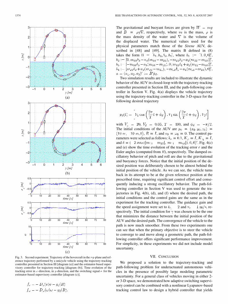
Fig. 3. Second experiment. Trajectory of the hovercraft in thexy-plane and ref-erence trajectory performed by a unicycle vehicle using the trajectory-trackingcontroller presented in Section III [diagram (a)] and the estimator-based super-visory controller for trajectory-tracking [diagram (b)]. Time evolution of thetracking error in x-direction, in y-direction, and the switching signal � for theestimator-based supervisory controller [diagram (c)].

The gravitational and buoyant forces are given byand , respectively, where is the mass, isthe mass density of the water and is the volume ofthe displaced water. The numerical values used for thephysical parameters match those of the Sirene AUV, de-scribed in [48] and [49]. The matrix B defined in (8)takes the form , where ,

,,,

.Two simulation results are included to illustrate the dynamic

behavior of the AUV in closed-loop with the trajectory-trackingcontroller presented in Section III, and the path-following con-troller in Section V. Fig. 4(a) displays the vehicle trajectoryusing the trajectory-tracking controller in the 3-D-space for thefollowing desired trajectory

with , , , and .The initial conditions of the AUV are

, , and . The control pa-rameters were selected as follows: , , ,and . Fig. 4(c)and (e) show the time evolution of the tracking error and theEuler angles (computed from ), respectively. The damped os-cillatory behavior of pitch and roll are due to the gravitationaland buoyancy forces. Notice that the initial position of the de-sired position was deliberately chosen to be almost behind theinitial position of the vehicle. As we can see, the vehicle turnsback in its attempt to be at the given reference position at theprescribed time, requiring significant control effort and conse-quently inducing a strong oscillatory behavior. The path-fol-lowing controller in Section V was used to generate the tra-jectories in Fig. 4(b), (d), and (f) where the desired path, theinitial conditions and the control gains are the same as in theexperiment for the tracking controller. The guidance gain andthe speed assignment were set to and , re-spectively. The initial condition for was chosen to be the onethat minimizes the distance between the initial position of theAUV and the desired path. The convergence of the vehicle to thepath is now much smoother. From these two experiments onecan see that when the primary objective is to steer the vehicleto converge to and move along a geometric path, the path-fol-lowing controller offers significant performance improvement.For simplicity, in these experiments we did not include modeluncertainty.

VII. CONCLUSION

We proposed a solution to the trajectory-tracking andpath-following problem for underactuated autonomous vehi-cles in the presence of possibly large modeling parametricuncertainty. For a general class of vehicles moving in either 2-or 3-D space, we demonstrated how adaptive switching supervi-sory control can be combined with a nonlinear Lyapunov-basedtracking control law to design a hybrid controller that yields


Fig. 4. Vehicle trajectory in 3-D space using the trajectory-tracking controller presented in Section III [diagram (a)], and the path-following controller [diagram(b)]. Time evolution of the position error e = (e ; e ; e ), the roll �, pitch �, and yaw Euler angles for the trajectory-tracking [diagrams (c), (e)], and thepath-following [diagrams (d), (f)].

global boundedness and convergence of the position trackingerror to a small neighborhood, and robustness to parametric

modeling uncertainty. We illustrated our results in the contextof two vehicle control applications: a hovercraft (moving on


a planar surface) and an underwater vehicle (moving in 3-Dspace). Simulations show that the control objectives were ac-complished.

An alternative approach to the Lyapunov-based controlscheme proposed in Section III consists in choosing an ad-equate point linked to the vehicle and then utilize outputfeedback linearization to design a simple controller that drivesthat point to the reference trajectory. See, for example, [10]for the case of unicycle-like mobile robots. For general un-deractuated vehicles, the stability of the zero-dynamics wouldhave to be established independently. This is an issue for futureresearch.

A problem that warrants further research is the control ofunderactuated vehicles with noise and in the presence of dis-turbances. Typical disturbances for marine vehicles include theones induced by wave, wind, and ocean current.

APPENDIX

Property 1: Let be nonzero and uni-formly bounded by . Then, there exists a vector thatmakes defined in (8) full-rank.

Proof: Pick , whereand is a positive constant to be selected shortly.

Defining , we conclude that

(40)

where we used the fact that the rank of a matrix does not changewhen it is multiplied by a nonsingular matrix. From the defi-nition of [see (6)] we conclude that each element of canbe bounded by . Much tighter boundscan be obtained for specific class of vehicles. For example, when

then . Assume now that . From(40), we conclude that B has full-rank if one can find at least one

minor determinant of nonzero. Considerthe one formed by the first, third, and forth columns, i.e.

(41)

where collects all the remaining terms and does not dependon . It follows now from the fact that each can be ar-bitrarily small by choosing (and consequently ) sufficientlarge, that (41) can be made nonzero and therefore B full-rank.If , the same conclusion about the full-rank of B can bemade by following the same reasoning but with if

, or for the case .

Lemma 1:Proof: Throughout this proof, to avoid cumbersome notation,

we will use , , , to denote , , , and , re-spectively. Note also that corresponds to the nominalmodel and therefore is equal to . The same applies forthe other model parameters. Consider the following exponen-tially weighted Lyapunov-like functions:

where is any positive constant that satisfies

(42)

Computing the time derivative of and along the solutionsof (2b), (3), and (16) for , we obtain

(43a)

(43b)

To prove (18a), consider the Lyapunov function

, which is the same as with . From (43) itfollows that: . Using theComparison Lemma [45] one concludes that (18a) holds with

and .To prove (18b), observe from (43a) and (42) that

Defining and taking an intervalon which , we have

and, therefore

Consequently


with . On the other hand, if for some, for all . Therefore

Inequality (18c) can be also concluded by applying the samearguments to (43b). In that case .

Lemma 2:Proof: Taking norms to defined in (20) and using

(17a) we conclude that

Also, from (17b) and (17c), a bound for given in (27) canbe computed as follows:

Using these two bounds in (26) and resorting to Young’sinequality it follows that for every positive constant ,

, satisfies

where we used the facts thatand

. Therefore, there existsufficiently small positive constants , , , andsufficiently large positive constants , such that

(44)

where in view of (29) and (30), the signals ,, , are defined

on , and is defined on . Applyingthe Comparison Lemma to (44) and using [46, Lemma 1]we conclude that is bounded on . Moreover, when

, converges to a ball of radius as. Standard signal chasing arguments can now be applied

to conclude that the signals , , and inclosed-loop system remain bounded. Furthermore, applying thesame arguments described in the proof of item ii) of Theorem1, one conclude that the tracking error convergesto a neighborhood of the origin that can be made arbitrarilysmall.

Derivation of (35): Using (16) for and the fact that, and ,

the time-derivative of in (34) can be written as

Using the Young’s inequality, after a straightforward but messycomputations, one can conclude that there exist a sufficiently


small and sufficiently large , suchthat for all , (35) holds with

REFERENCES

[1] H. Goldstein, Classical Mechanics, 2nd ed. Reading, MA: Addison-Wesley, 1980, 672 pages.

[2] J. T.-Y. Wen, “Control of nonholonomic systems,” in The ControlHandbook, W. S. Levine, Ed. Boca Raton, FL: CRC and IEEE ,1996, pp. 1359–1368.

[3] M. Reyhanoglu, A. van der Schaft, N. H. McClamroch, and I. Kol-manovsky, “Dynamics and control of a class of underactuated me-chanical systems,” IEEE Trans. Autom. Control, vol. 44, no. 9, pp.1663–1671, 1999.

[4] F. Bullo, N. E. Leonard, and A. D. Lewis, “Controllability and motionalgorithms for underactuated lagrangian systems on lie groups,” IEEETrans. Autom. Control, vol. 45, no. 8, pp. 1437–1454, 2000.

[5] J. S. Shamma and J. R. Cloutier, “Gain-scheduled missile autopilot de-sign using linear parameter varying transformations,” J. Guid. ControlDyn., vol. 16, no. 2, pp. 256–263, 1993.

[6] I. Kaminer, A. Pascoal, E. Hallberg, and C. Silvestre, “Trajectorytracking controllers for autonomous vehicles: An integrated approachto guidance and control,” J. Guid. Control Dyn., vol. 21, no. 1, pp.29–38, 1998.

[7] W. J. Rugh and J. S. Shamma, “Research on gain-scheduling,” Auto-matica, vol. 36, no. 10, pp. 1401–1425, 2000.

[8] T. Koo and S. Sastry, “Output tracking control design of a helicoptermodel based on approximate linearization,” in Proc. 37th Conf. Deci-sion Control, Tampa, FL, Dec. 1998, pp. 3635–3640.

[9] S. Al-Hiddabi and N. McClamroch, “Tracking and maneuver regula-tion control for nonlinear nonminimum phase systems: Application toflight control,” IEEE Trans. Contr. Syst. Technol., vol. 10, no. 6, pp.780–792, 2002.

[10] J. R. T. Lawton, R. W. Beard, and B. J. Young, “A decentralized ap-proach to formation maneuvers,” IEEE Trans. Robot. Autom., vol. 19,no. 6, pp. 933–941, 2003.

[11] A. Isidori, Nonlinear Control Systems, 3rd ed. London, U.K.:Springer-Verlag, 1989.

[12] J. M. Godhavn, “Nonlinear tracking of underactuated surface vessels,”in Proc. 35th Conf. Decision Control, Kobe, Japan, Dec. 1996, pp.975–980.

[13] K. Y. Pettersen and H. Nijmeijer, “Global practical stabilizationand tracking for an underactuated ship—A combined averaging andbackstepping approach,” in Proc. IFAC Conf. Syst. Structure Control,Nantes, France, Jul. 1998, pp. 59–64.

[14] F. Alonge, F. D’Ippolito, and F. Raimondi, “Trajectory tracking of un-deractuated underwater vehicles,” in Proc. 40th Conf. Decision Con-trol, Orlando, FL, USA, Dec. 2001.

[15] Z.-P. Jiang, “Global tracking control of underactuated ships by Lya-punov’s direct method,” Automatica, vol. 38, pp. 301–309, 2002.

[16] A. Behal, D. Dawson, W. Dixon, and Y. Fang, “Tracking and regu-lation control of an underactuated surface vessel with nonintegrabledynamics,” IEEE Trans. Autom. Control, vol. 47, no. 3, pp. 495–500,Mar. 2002.

[17] K. D. Do, Z. P. Jiang, and J. Pan, “Underactuated ship global trackingunder relaxed conditions,” IEEE Trans. Autom. Control, vol. 47, no. 9,pp. 1529–1536, Sep. 2002.

[18] K. D. Do, “Universal controllers for stabilization and tracking of un-deractuated ships,” Syst. Control Lett., vol. 47, pp. 299–317, 2002.

[19] K. Y. Pettersen and H. Nijmeijer, “Tracking control of an underactu-ated ship,” IEEE Trans. Contr. Syst. Technol., vol. 11, no. 1, pp. 52–61,2003.

[20] E. Frazzoli, M. Dahleh, and E. Feron, “Trajectory tracking control de-sign for autonomous helicopters using a backstepping algorithm,” inProc. 2000 Amer. Contr. Conf., Chicago, IL, Jun. 2000.

[21] J. P. Hespanha, D. Liberzon, and A. S. Morse, “Supervision of integral-input-to-state stabilizing controllers,” Automatica, vol. 38, no. 8, pp.1327–1335, 2002.

[22] M. Krstic, I. Kanellakopoulos, and P. Kokotovic, Nonlinear and Adap-tive Control Design. New York: Wiley , 1995.

[23] S. Sastry and M. Bodson, Adaptive Control: Stability, Convergence,and Robustness. Englewood Cliffs, NJ: Prentice-Hall, 1989.

[24] P. A. Ioannou and J. Sun, Robust Adaptive Control.. EnglewoodCliffs, NJ: Prentice-Hall, 1996.

[25] J. P. Hespanha, D. Liberzon, and A. S. Morse, “Overcoming the lim-itations of adaptive control by means of logic-based switching,” Syst.Contr. Lett., vol. 49, no. 1, pp. 49–65, 2003.

[26] A. S. Morse, “Supervisory control of families of linear set-point con-trollers part 1: Exact matching,” IEEE Trans. Autom. Control, vol. 41,no. 10, pp. 1413–1431, 1996.

[27] J. P. Hespanha and A. S. Morse, “Certainty equivalence implies de-tectability,” Syst. Control Lett., vol. 36, no. 1, pp. 1–13, 1999.

[28] J. P. Hespanha, D. Liberzon, and A. S. Morse, “Logic-based switchingcontrol of a nonholonomic system with parametric modeling uncer-tainty,” Syst. Control Lett., vol. 38, no. 3, pp. 167–177, 1999.

[29] G. Chang, J. Hespanha, A. S. Morse, M. Netto, and R. Ortega, “Super-visory field-oriented control of induction motors with uncertain rotorresistance,” Int. J. Adapt. Contr. Signal Process., vol. 15, no. 3, pp.353–375, 2001.

[30] D. Angeli and E. Mosca, “Lyapunov-based switching supervisory con-trol of nonlinear uncertain systems,” IEEE Trans. Autom. Control, vol.47, no. 3, pp. 500–505, 2002.

[31] F. Bullo, “Stabilization of relative equilibria for underactuated systemson riemannian manifolds,” Automatica, vol. 36, pp. 1819–1834, 2000.

[32] C. Samson, “Path-following and time-varying feedback stabilizationof a wheeled mobile robot,” in Proc. ICARCV 92, Singapore, 1992, pp.RO-13.1.1–RO-13.1.5.

[33] C. C. d. Wit, H. Khennouf, C. Samson, and O. J. Sordalen, “Nonlinearcontrol design for mobile robots,” in Recent Trends in Mobile Robots,ser. World Scientific Ser. Robot. Automated Syst., Y. F. Zheng, Ed. :, 1993, vol. 11, pp. 121–156.

[34] C. Samson, “Control of chained systems: Application to path followingand time-varying point-stabilization of mobile robots,” IEEE Trans.Autom. Control, vol. 40, no. 1, pp. 64–77, 1995.

[35] Z.-P. Jiang and H. Nijmeijer, “A recursive technique for tracking con-trol of nonholonomic systems in chained form,” IEEE Trans. Autom.Control, vol. 44, no. 2, pp. 265–279, 1999.

[36] C. Altafini, “Following a path of varying curvature as an outputregulation problem,” IEEE Trans. Autom. Control, vol. 47, no. 9, pp.1551–1556, 2002.

[37] J. Hauser and R. Hindman, “Aggressive flight maneuvers,” inProc. 36th Conf. Decision Control, San Diego, CA, Dec. 1997, pp.4186–4191.

[38] P. Encarnaçaao and A. M. Pascoal, “3D path following control of au-tonomous underwater vehicles,” in Proc. 39th Conf. Decision Control,Sydney, Australia, Dec. 2000.

[39] R. Skjetne, T. I. Fossen, and P. Kokotovic, “Robust output maneu-vering for a class of nonlinear systems,” Automatica, vol. 40, no. 3,pp. 373–383, 2004.

[40] A. P. Aguiar, D. B. Dacic, J. P. Hespanha, and P. Kokotovic, “Path-fol-lowing or reference-tracking? An answer based on limits of perfor-mance,” in Proc. 5th IFAC/EURON Symp. Intell. Auton. Veh., Lisbon,Portugal, Jul. 2004.

[41] A. P. Aguiar, J. P. Hespanha, and P. Kokotovic, “Path-following fornon-minimum phase systems removes performance limitations,” IEEETrans. Autom. Control, vol. 50, no. 2, pp. 234–239, 2005.

[42] A. P. Aguiar and J. P. Hespanha, “Position tracking of underactuatedvehicles,” in Proc. 2003 Amer. Contr. Conf., Denver, CO, Jun. 2003.

[43] A. P. Aguiar, L. Cremean, and J. P. Hespanha, “Position tracking fora nonlinear underactuated hovercraft: Controller design and experi-mental results,” in Proc. 42nd Conf. Decision Control, HI, Dec. 2003.


[44] A. P. Aguiar and J. P. Hespanha, “Logic-based switching control fortrajectory-tracking and path-following of underactuated autonomousvehicles with parametric modeling uncertainty,” in Proc. 2004 Amer.Contr. Conf., Boston, MA, Jun. 2004.

[45] H. K. Khalil, Nonlinear Systems, 2nd ed. Englewood Cliffs, NJ: Pren-tice-Hall, 1996.

[46] A. S. Morse, “Towards a unified theory of parameter adaptive control:Tunability,” IEEE Trans. Autom. Control, vol. 35, no. 9, pp. 1002–1012,1990.

[47] L. Cremean, W. Dumbar, D. van Gogh, J. Hickey, E. Klavins, J.Meltzer, and R. Murray, “The caltech multi-vehicle wireless testbed,”in Proc. 41st Conf. Decision Control, Las Vegas, NV, Dec. 2002.

[48] A. P. Aguiar and A. M. Pascoal, “Modeling and control of an au-tonomous underwater shuttle for the transport of benthic laboratories,”in Proc. Oceans’97 Conf., Halifax, Nova Scotia, Canada, Oct. 1997.

[49] A. P. Aguiar, “Nonlinear motion control of nonholonomic and under-actuated systems,” Ph.D. dissertation, Dep. Elect. Eng., Instituto Supe-rior Técnico (IST), Lisbon, Portugal, 2002.

A. Pedro Aguiar (S’95–A’00–M’02) received the Licenciatura, M.S. and Ph.D.degrees in electrical and computer engineering from the Instituto Superior Téc-nico, Technical University of Lisbon, Portugal, in 1994, 1998, and 2002, respec-tively.

From 2002 to 2005, he was a Postdoctoral Researcher with the Centerfor Control, Dynamical-Systems, and Computation, University of California,Santa Barbara. Currently, he holds an Invited Assistant Professor position withthe Department of Electrical and Computer Engineering, Instituto SuperiorTécnico, and a Senior Researcher position with the Institute for Systems andRobotics, Instituto Superior Técnico (ISR/IST). His research interests includemodeling, control, navigation, and guidance of autonomous vehicles; nonlinearcontrol; switched and hybrid systems; tracking, path-following; performancelimitations; nonlinear observers; the integration of machine vision with feed-back control; and coordinated/cooperative control of multiple autonomousrobotic vehicles. Further information related to his research can be found athttp://www.users.isr.ist.utl.pt/~pedro.

João P. Hespanha (S’95–A’98–M’00–SM’02) received the Licenciaturain electrical and computer engineering from the Instituto Superior Técnico,Lisbon, Portugal, in 1991 and the M.S. and Ph.D. degrees in electrical engi-neering and applied science from Yale University, New Haven, CT, in 1994and 1998, respectively.

He currently holds an Associate Professor position with the Department ofElectrical and Computer Engineering, University of California, Santa Barbara.From 1999 to 2001, he was an Assistant Professor with the University ofSouthern California, Los Angeles. He is the Associate Director for the Centerfor Control, Dynamical-Systems, and Computation (CCDC) and an executivecommittee member for the Institute for Collaborative Biotechnologies (ICB), anArmy sponsored University Affiliated Research Center (UARC). His researchinterests include hybrid and switched systems; the modeling and control ofcommunication networks; distributed control over communication networks(also known as networked control systems); the use of vision in feedbackcontrol; stochastic modeling in biology; and the control of haptic devices. Heis the author of more than 100 technical papers and the PI and co-PI in severalfederally funded projects. More information about his research can be foundat http://www.ece.ucsb.edu/~hespanha.

Dr. Hespanha is the recipient of Yale University’s Henry Prentiss BectonGraduate Prize for exceptional achievement in research in Engineering andApplied Science, a National Science Foundation CAREER Award, the 2005Automatica Theory/Methodology Best Paper prize, and the Best Paper awardat the 2nd International Conference on Intelligent Sensing and Informa-tion Processing. Since 2003, he has been an Associate Editor of the IEEETRANSACTIONS ON AUTOMATIC CONTROL.

Date post:	19-Sep-2018
Category:	Documents
Upload:	ngoanh
View:	231 times
Download:	0 times

1362 IEEE TRANSACTIONS ON AUTOMATIC...

Documents