Page 1
7/17/2019 13_Chapter One - Six
http://slidepdf.com/reader/full/13chapter-one-six 1/34
CHAPTER ONE
1. INTRODUCTION
Cooling tower are widely used in large air-conditioning installations to recycle
condenser cooling tower. The performance of cooling towers are often
expressed as Number of Transfer Unit (NTU).
A widely used method of calculating NTU is based on Merkel’s theory.
The theory is applicable to both counter flow and cross flow direct-contact
forced-draft air-water cooling towers as described by Stoecker and Jones
(1982).
Manual calculation of NTU is tedious and time-consuming. In this
research, computerized calculation are made to calculate the NTU of cross
flow cooling towers using Stoecker and Jones (1982), for a range of tower inlet
water temperature (tw1), outlet water temperature (tw2), ambient air wet bulb
temperature (twB) and ratio of water to air mass flow rate (L/G).
Multi-linear regression is then made to obtain correlations in the form
of :
NTU = a0. tw1a1.tw2a2.twba3(L/G)a4
Page 2
7/17/2019 13_Chapter One - Six
http://slidepdf.com/reader/full/13chapter-one-six 2/34
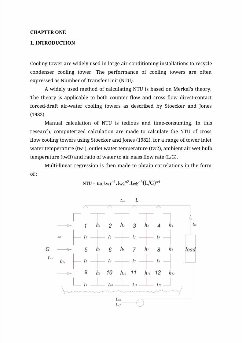
Figure 1.1 A cross flow cooling tower by dividing it into sections.
. Objective
To obtain theoretical correlations for cross flow cooling towers for the tower NTU as a
function of inlet water temperature, outlet water temperature, ambient air wet bulb
temperature, air flow rate and water flow rate.
1.2 Scope
Steady-state analysis of crossflow air-water cooling towers
Use of Merkel theory
Page 3
7/17/2019 13_Chapter One - Six
http://slidepdf.com/reader/full/13chapter-one-six 3/34
CHAPTER TWO
2. LITERATURE REVIEW
Cooling towers are widely used in air-conditioning applications for reducing the
temperature of circulating water for reuse in condensers. A cooling tower is an
evaporative cooling device where a circulating water is cooled by direct contact
with atmospheric air, where some of water is evaporated. Direct-contact
forced-draft air-water cooling towers involve the transfer of mass and hear
between the hot water and ambient air flowing in counter flow and cross flow
configurations.
A simplified cooling tower analysis is often made using Merkel’s (1925)
theory. The model is based on the enthalpy difference between the saturated air
enthalpy or the air water interface and the enthalpy of the surrounding air as the
driving potential for energy transfer.
Baker and Shryrock (1961) have discussed Merkel’s theory and suggested
the use of on offset ratio refers to the ratio between the true enthalpy potential
and the difference in the air/water interface temperature and the bulk water
temperature. They also studied the effects of neglecting the evaporative water
loss and the liquid side thermal resistance on the cooling tower performance.
The liquid side thermal resistance was considered in a cross flow cooling
tower analysis, they have also shown that the true driving potential was lower
than that without the liquid side thermal resistance. By considering
evaporative water loss and the liquid side thermal resistance, the resulting
“true” NTUs were also shown to be greater than those calculated using
Merkel’s theory for an experimental cross-flow cooling tower.
Osterle (1991) presented a tower model for which the Merkel equations
were corrected to account for mass of water lost by evaporation. The corrected
NTUs were evaluated by solving a set of differential equations.
Page 4
7/17/2019 13_Chapter One - Six
http://slidepdf.com/reader/full/13chapter-one-six 4/34
Majumdar et. al (1983) have developed a two –dimensional model that
coupled the thermodynamics and hydrodynamics for simulating cooling
tower performance in either a counter-flow or cross-flow configuration. The
governing partial differential equations have been solved using finitedifference techniques in a computer code.
Bernier (1994) analysing the cooling tower heat rejection performance
must be obtained experimentally, where the NTU is evaluated using several
theories and models. The product of Ka in the NTU definition represents
average values of K and a in the tower, where K is the mass transfer
coefficient, and a is the air/water contact area per unit of tower volume. The
simplest and widely used theory for cooling tower analysis has been proposed
by Merkel in 1925.
Maiya (1995) analysing the performance of modified counter-flow
cooling tower. Bedekar (1998) investigation on the performance of a
counter-flow, packed-bed cooling tower.
Page 5
7/17/2019 13_Chapter One - Six
http://slidepdf.com/reader/full/13chapter-one-six 5/34
CHAPTER THREE
3. METHODOLOGY
In a cooling tower, heat and mass are transferred from water to air. A cooling tower
with an effectiveness of 100% would exhaust saturated air from the tower at the
temperature of the entering water. In actual towers, the air leaves at a temperature
less than the entering water temperature and a relative humidity less than 100%
because the airflow is too high and the heat transfer area is too small. Effectiveness,
εa, is defined10 in terms of the enthalpy of moist air as follows:
ε a = (hi,in -hi,out) / (t w2 –t w1) (3-1)
In Equation (1), hi,in and hi,out are the enthalpies of the air into and out of the tower, and
t w2 is the enthalpy of air saturated with water at the inlet water temperature.
Effectiveness is a dimensionless variable which can be determined from knowledge of
only two additional dimensionless variables, NTU.
NTU = (h c A) / (C pmL ) (3-2)
From Equation (3-7), NTU depends on the heat transfer coefficient, h c, the heat transfer
surface area, A, and the specific heat, C pm. Energy efficient cooling towers with large heat
transfer surfaces and small fans might have nominal NTU values of 4.5 or more. Low initial
cost towers with small heat transfer surfaces and large fans might have nominal NTU
values of 1.5 or less.
Since h c depends on the airflow rate and the water flow rate, the NTU value of a tower
Page 6
7/17/2019 13_Chapter One - Six
http://slidepdf.com/reader/full/13chapter-one-six 6/34
operating at off-design conditions will not be the same as the NTU value at design
conditions. An empirical equation useful for predicting NTU at off-design conditions is:
NTU = = 4.19 (3-3)
The constants, a, m, and n, in Equation (3-3) are to be determined from published
performance data. In some cases, this data is unavailable.
The heat exchangers are usually characterized by the Number of Transfer Unit NTU.
Since the tower has similar hydrothermal operation, then it is possible to characterize
the tower performance using the NTU as following.
Since NTU are known for a particular cooling tower, the cooling tower
performance can be predicted at any operating condition using;
Multi Linear Regression ;
NTU = a0. tw1a1.tw2
a2.twba3(L/G)a4 (3-4)
Estimate;
NTU = 1 -number of unit transfer
tw1 = 37oC -entering water temperature
tw2 = 35oC -leaving water temperature
twb = 25oC -temperature wet bulb entering air
= 1.0
n x n = 10 x 10 -dividing section in cross flow cooling tower
calculate using eq.(3-9)
1= c.(37)c(35)c(25)c(1.0)c
a=9.2592 * 10-3 …….into eq.(3.9) to get the actual NTU
So,
Page 7
7/17/2019 13_Chapter One - Six
http://slidepdf.com/reader/full/13chapter-one-six 7/34
NTU actual = 0.0101
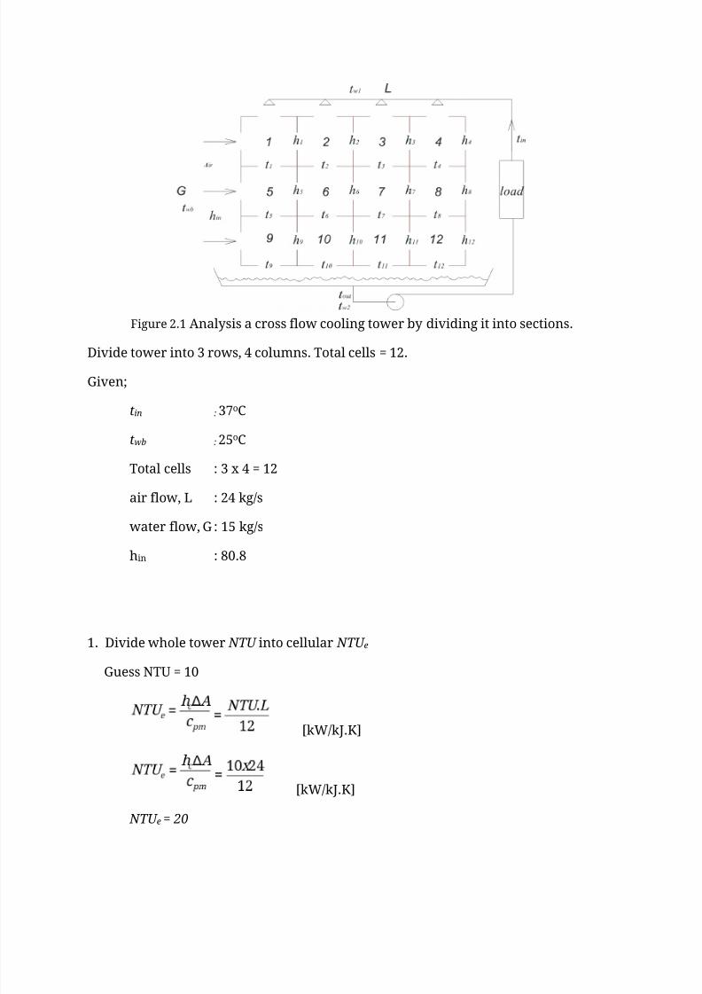
Although the counter flow cooling tower is widely used in industrial services, another
configuration is the cross flow tower, in which the air passes horizontally through the
falling water sprays. Cooling towers used for air-conditioning systems are often
located atop buildings, and cross flow cooling tower usually has a lower profile,
which lends itself better to architectural treatment.
The same principles of heat and mass transfer and balance of energy apply to a
cross flow tower and to the counter flow type, but the geometric treatment of the
cross flow tower is different. Figure 3-1 showns a cross flow tower divided into 12
sections for purposes of analysis. Water enters the top at a temperature tin while air
enters from the left with an enthalpy hin. In section 1 air enters at enthalpy hin and
leaves with enthalpy h1. Also in section 1 water entera at tin and leaves at t1. The
enthalpy of air entering section 2 is h1, and the water enters section 5 with a
temperature t1. The temperature of water leaving sections 9, 10, 11, and 12 at the
bottom of the tower are t9, t10, t11, and t12, respectively. These temperatures are all
different, and the streams combine to form one stream of temperature tout.
If the value of hc A/C pm is known for the entire cooling tower, the outlet water
temperature can be predicted when the inlet water temperature, inlet air enthalpy,
and the flow rates of water and air are known. The tower can be divided into a
number of small increments (12 increment, for example, in Fig 2-1) and (hc A/C pm )/12
assigned to each increment. Let
=
Page 8
7/17/2019 13_Chapter One - Six
http://slidepdf.com/reader/full/13chapter-one-six 8/34
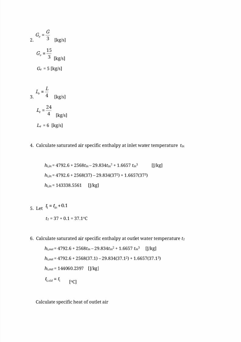
Figure 2.1 Analysis a cross flow cooling tower by dividing it into sections.
Divide tower into 3 rows, 4 columns. Total cells = 12.
Given;
tin : 37oC
twb : 25oC
Total cells : 3 x 4 = 12
air flow, L : 24 kg/s
water flow, G : 15 kg/s
hin : 80.8
1. Divide whole tower NTU into cellular NTU e
Guess NTU = 10
[kW/kJ.K]
[kW/kJ.K]
NTU e = 20
Page 9
7/17/2019 13_Chapter One - Six
http://slidepdf.com/reader/full/13chapter-one-six 9/34
2. [kg/s]
[kg/s]
Ge = 5 [kg/s]
3. [kg/s]
[kg/s]
Le = 6 [kg/s]
4. Calculate saturated air specific enthalpy at inlet water temperature tin
hi,in = 4792.6 + 2568tin – 29.834tin2 + 1.6657 tin
3 [J/kg]
hi,in = 4792.6 + 2568(37) – 29.834(372) + 1.6657(373)
hi,in = 143338.5561 [J/kg]
5. Let
t1 = 37 + 0.1 = 37.1oC
6. Calculate saturated air specific enthalpy at outlet water temperature t1
hi,out = 4792.6 + 2568tin – 29.834tin2 + 1.6657 tin
3 [J/kg]
hi,out = 4792.6 + 2568(37.1) – 29.834(37.12) + 1.6657(37.13)
hi,out = 144060.2397 [J/kg]
[oC]
Calculate specific heat of outlet air
Page 10
7/17/2019 13_Chapter One - Six
http://slidepdf.com/reader/full/13chapter-one-six 10/34
[J/kg]
h1 = 153938.8348 [J/kg]
Heat gain by air
[W]
dq = 5 (162-80.8) [W]
dq = 438833.0088 [W]
equals heat loss from falling water:
[oC]
[oC]
t1 = 16.0333 [oC]
7. If repeat step 6.
t1 - t1,old = 16.0333 - 37.1
t1 - t1,old = -21.0667
8. Repeat calculations (steps 4–6) for the other cells.
9. At the bottom of tower calculate the average exit water temperature tout
Page 11
7/17/2019 13_Chapter One - Six
http://slidepdf.com/reader/full/13chapter-one-six 11/34
CHAPTER FOUR
4. DATA ANALYSIS AND RESULTS
A computer program has been written to calculate the NTU of cross flow cooling
towers using Merkel’s theory as described by Stocker and Jones (1982). The inputs to
the program are inlet water temperature (tw1), outlet water temperature (tw2),
Page 12
7/17/2019 13_Chapter One - Six
http://slidepdf.com/reader/full/13chapter-one-six 12/34
ambient air wet bulb temperature (twB) and the ratio of water to air mass flow rate
(L/G). The program calculates the NTU as described in Chapter 3.
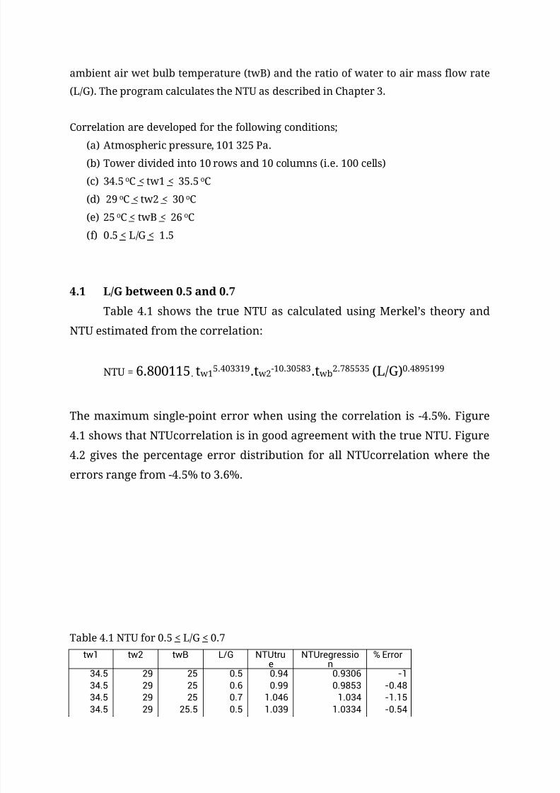
Correlation are developed for the following conditions;
(a) Atmospheric pressure, 101 325 Pa.
(b) Tower divided into 10 rows and 10 columns (i.e. 100 cells)
(c) 34.5 oC < tw1 < 35.5 oC
(d) 29 oC < tw2 < 30 oC
(e) 25 oC < twB < 26 oC
(f) 0.5 < L/G < 1.5
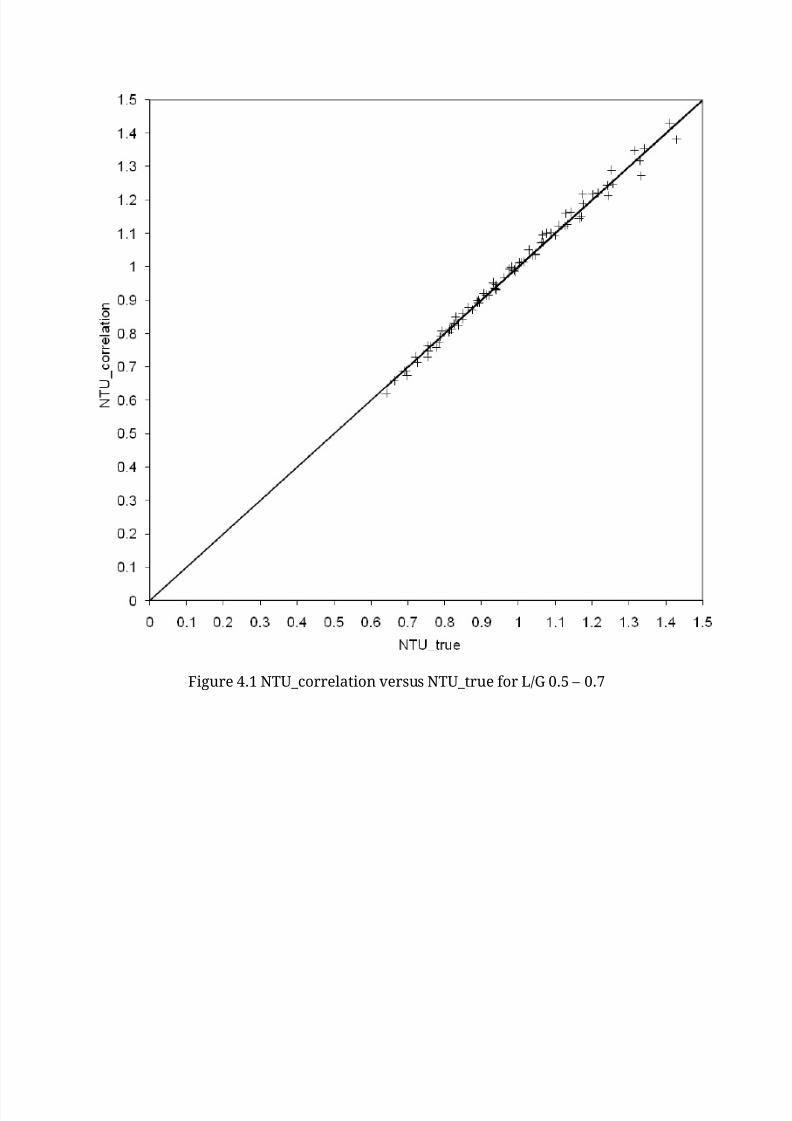
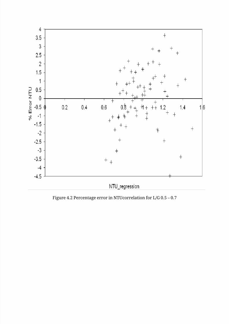
4.1 L/G between 0.5 and 0.7
Table 4.1 shows the true NTU as calculated using Merkel’s theory and
NTU estimated from the correlation:
NTU = 6.800115. tw15.403319.tw2
-10.30583.twb2.785535 (L/G)0.4895199
The maximum single-point error when using the correlation is -4.5%. Figure4.1 shows that NTUcorrelation is in good agreement with the true NTU. Figure
4.2 gives the percentage error distribution for all NTUcorrelation where the
errors range from -4.5% to 3.6%.
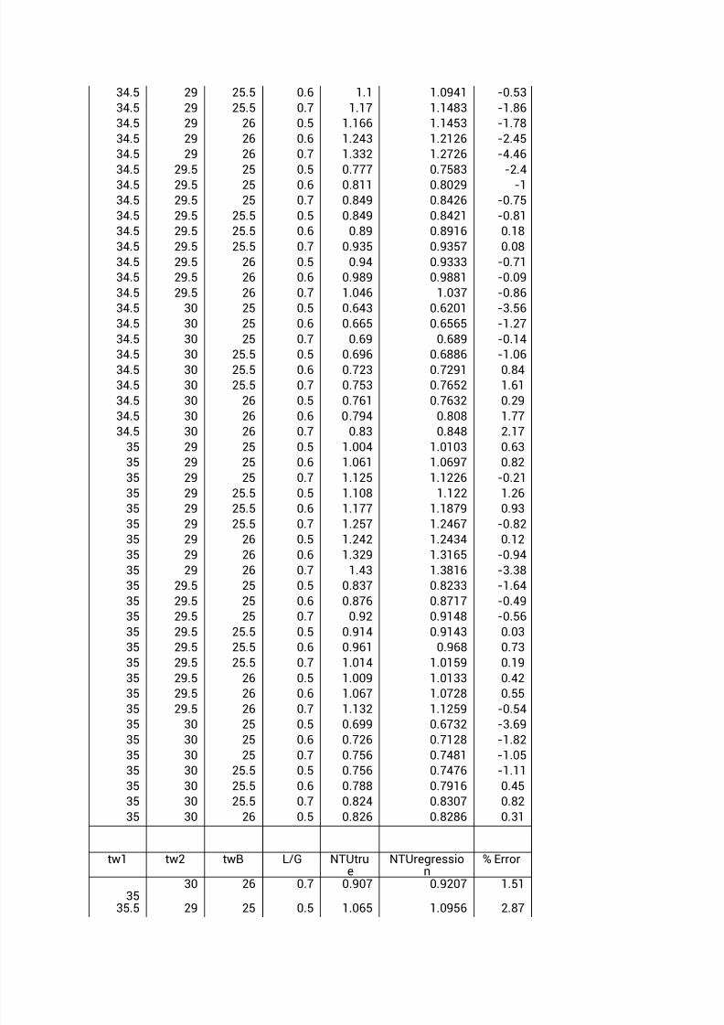
Table 4.1 NTU for 0.5 < L/G < 0.7
tw1 tw2 twB L/G NTUtrue
NTUregression
% Error
34.5 29 25 0.5 0.94 0.9306 -1
34.5 29 25 0.6 0.99 0.9853 -0.48
34.5 29 25 0.7 1.046 1.034 -1.1534.5 29 25.5 0.5 1.039 1.0334 -0.54
Page 13
7/17/2019 13_Chapter One - Six
http://slidepdf.com/reader/full/13chapter-one-six 13/34
34.5 29 25.5 0.6 1.1 1.0941 -0.53
34.5 29 25.5 0.7 1.17 1.1483 -1.86
34.5 29 26 0.5 1.166 1.1453 -1.78
34.5 29 26 0.6 1.243 1.2126 -2.45
34.5 29 26 0.7 1.332 1.2726 -4.46
34.5 29.5 25 0.5 0.777 0.7583 -2.4
34.5 29.5 25 0.6 0.811 0.8029 -1
34.5 29.5 25 0.7 0.849 0.8426 -0.75
34.5 29.5 25.5 0.5 0.849 0.8421 -0.81
34.5 29.5 25.5 0.6 0.89 0.8916 0.18
34.5 29.5 25.5 0.7 0.935 0.9357 0.08
34.5 29.5 26 0.5 0.94 0.9333 -0.71
34.5 29.5 26 0.6 0.989 0.9881 -0.09
34.5 29.5 26 0.7 1.046 1.037 -0.86
34.5 30 25 0.5 0.643 0.6201 -3.56
34.5 30 25 0.6 0.665 0.6565 -1.27
34.5 30 25 0.7 0.69 0.689 -0.14
34.5 30 25.5 0.5 0.696 0.6886 -1.0634.5 30 25.5 0.6 0.723 0.7291 0.84
34.5 30 25.5 0.7 0.753 0.7652 1.61
34.5 30 26 0.5 0.761 0.7632 0.29
34.5 30 26 0.6 0.794 0.808 1.77
34.5 30 26 0.7 0.83 0.848 2.17
35 29 25 0.5 1.004 1.0103 0.63
35 29 25 0.6 1.061 1.0697 0.82
35 29 25 0.7 1.125 1.1226 -0.21
35 29 25.5 0.5 1.108 1.122 1.26
35 29 25.5 0.6 1.177 1.1879 0.93
35 29 25.5 0.7 1.257 1.2467 -0.82
35 29 26 0.5 1.242 1.2434 0.1235 29 26 0.6 1.329 1.3165 -0.94
35 29 26 0.7 1.43 1.3816 -3.38
35 29.5 25 0.5 0.837 0.8233 -1.64
35 29.5 25 0.6 0.876 0.8717 -0.49
35 29.5 25 0.7 0.92 0.9148 -0.56
35 29.5 25.5 0.5 0.914 0.9143 0.03
35 29.5 25.5 0.6 0.961 0.968 0.73
35 29.5 25.5 0.7 1.014 1.0159 0.19
35 29.5 26 0.5 1.009 1.0133 0.42
35 29.5 26 0.6 1.067 1.0728 0.55
35 29.5 26 0.7 1.132 1.1259 -0.54
35 30 25 0.5 0.699 0.6732 -3.69
35 30 25 0.6 0.726 0.7128 -1.82
35 30 25 0.7 0.756 0.7481 -1.05
35 30 25.5 0.5 0.756 0.7476 -1.11
35 30 25.5 0.6 0.788 0.7916 0.45
35 30 25.5 0.7 0.824 0.8307 0.82
35 30 26 0.5 0.826 0.8286 0.31
tw1 tw2 twB L/G NTUtrue
NTUregression
% Error
35
30 26 0.7 0.907 0.9207 1.51
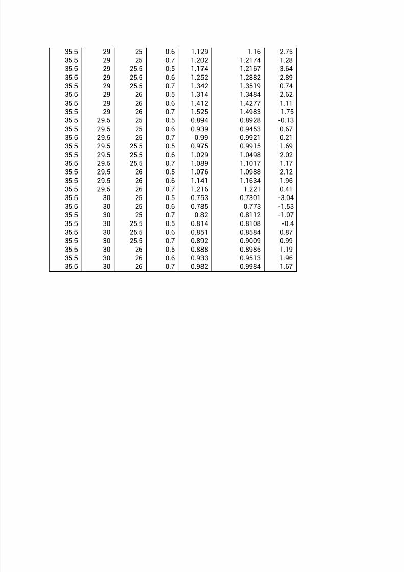
35.5 29 25 0.5 1.065 1.0956 2.87
Page 14
7/17/2019 13_Chapter One - Six
http://slidepdf.com/reader/full/13chapter-one-six 14/34
35.5 29 25 0.6 1.129 1.16 2.75
35.5 29 25 0.7 1.202 1.2174 1.28
35.5 29 25.5 0.5 1.174 1.2167 3.64
35.5 29 25.5 0.6 1.252 1.2882 2.89
35.5 29 25.5 0.7 1.342 1.3519 0.74
35.5 29 26 0.5 1.314 1.3484 2.62
35.5 29 26 0.6 1.412 1.4277 1.11
35.5 29 26 0.7 1.525 1.4983 -1.75
35.5 29.5 25 0.5 0.894 0.8928 -0.13
35.5 29.5 25 0.6 0.939 0.9453 0.67
35.5 29.5 25 0.7 0.99 0.9921 0.21
35.5 29.5 25.5 0.5 0.975 0.9915 1.69
35.5 29.5 25.5 0.6 1.029 1.0498 2.02
35.5 29.5 25.5 0.7 1.089 1.1017 1.17
35.5 29.5 26 0.5 1.076 1.0988 2.12
35.5 29.5 26 0.6 1.141 1.1634 1.96
35.5 29.5 26 0.7 1.216 1.221 0.41
35.5 30 25 0.5 0.753 0.7301 -3.0435.5 30 25 0.6 0.785 0.773 -1.53
35.5 30 25 0.7 0.82 0.8112 -1.07
35.5 30 25.5 0.5 0.814 0.8108 -0.4
35.5 30 25.5 0.6 0.851 0.8584 0.87
35.5 30 25.5 0.7 0.892 0.9009 0.99
35.5 30 26 0.5 0.888 0.8985 1.19
35.5 30 26 0.6 0.933 0.9513 1.96
35.5 30 26 0.7 0.982 0.9984 1.67
Page 15
7/17/2019 13_Chapter One - Six
http://slidepdf.com/reader/full/13chapter-one-six 15/34
Figure 4.1 NTU_correlation versus NTU_true for L/G 0.5 – 0.7
Page 16
7/17/2019 13_Chapter One - Six
http://slidepdf.com/reader/full/13chapter-one-six 16/34
Figure 4.2 Percentage error in NTUcorrelation for L/G 0.5 – 0.7
Page 17
7/17/2019 13_Chapter One - Six
http://slidepdf.com/reader/full/13chapter-one-six 17/34
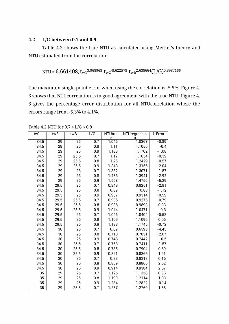
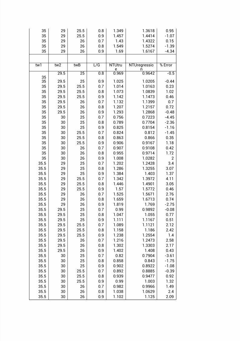
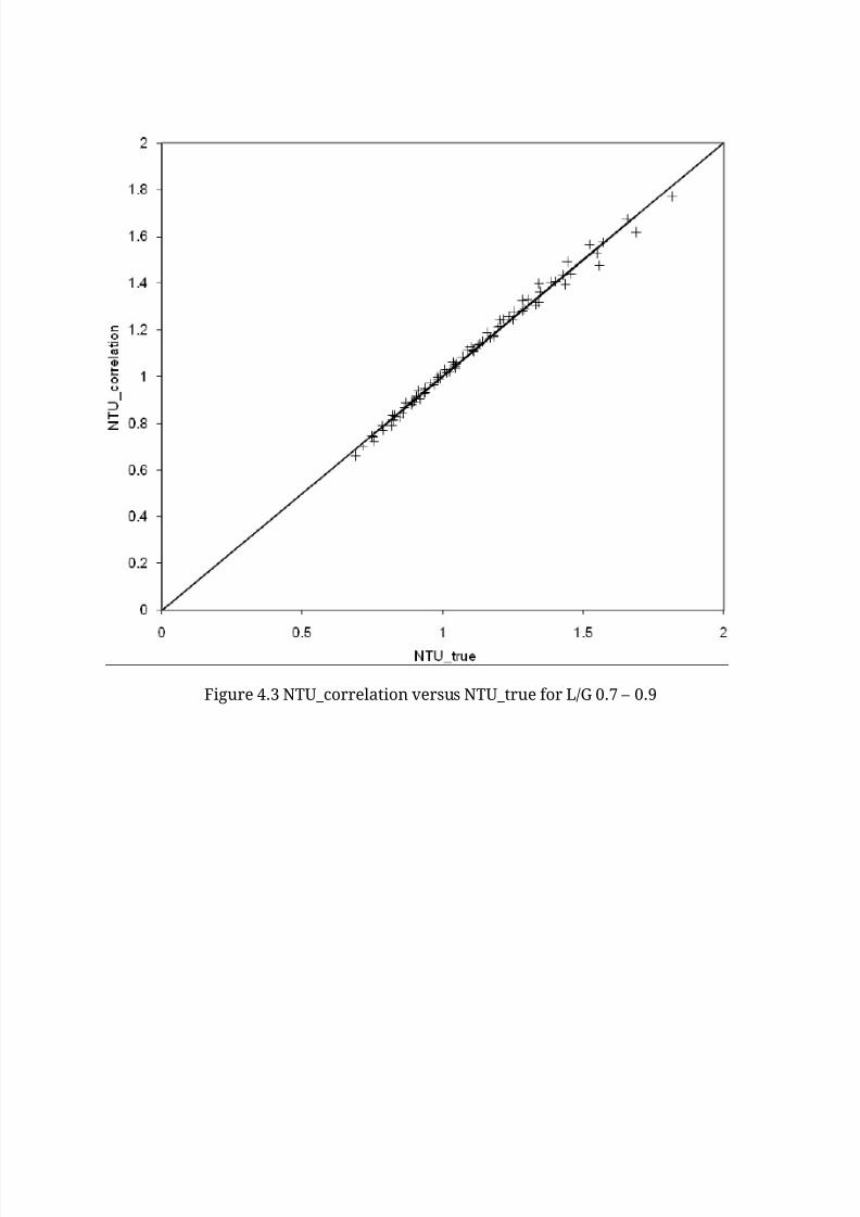
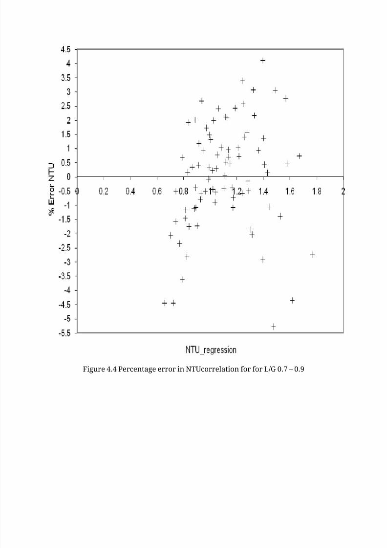
4.2 L/G between 0.7 and 0.9
Table 4.2 shows the true NTU as calculated using Merkel’s theory and
NTU estimated from the correlation:
NTU = 6.661408. tw13.968963.tw2
-8.622578.twb2.638664(L/G)0.3987166
The maximum single-point error when using the correlation is -5.5%. Figure 4.
3 shows that NTUcorrelation is in good agreement with the true NTU. Figure 4.
3 gives the percentage error distribution for all NTUcorrelation where the
errors range from -5.3% to 4.1%.
Table 4.2 NTU for 0.7 < L/G < 0.9
tw1 tw2 twB L/G NTUtrue
NTUregression
% Error
34.5 29 25 0.7 1.046 1.0367 -0.89
34.5 29 25 0.8 1.11 1.1056 -0.4
34.5 29 25 0.9 1.183 1.1702 -1.08
34.5 29 25.5 0.7 1.17 1.1654 -0.39
34.5 29 25.5 0.8 1.25 1.2429 -0.57
34.5 29 25.5 0.9 1.343 1.3156 -2.04
34.5 29 26 0.7 1.332 1.3071 -1.8734.5 29 26 0.8 1.436 1.3941 -2.92
34.5 29 26 0.9 1.558 1.4756 -5.29
34.5 29.5 25 0.7 0.849 0.8251 -2.81
34.5 29.5 25 0.8 0.89 0.88 -1.12
34.5 29.5 25 0.9 0.937 0.9314 -0.59
34.5 29.5 25.5 0.7 0.935 0.9276 -0.79
34.5 29.5 25.5 0.8 0.986 0.9893 0.33
34.5 29.5 25.5 0.9 1.044 1.0471 0.3
34.5 29.5 26 0.7 1.046 1.0404 -0.53
34.5 29.5 26 0.8 1.109 1.1096 0.06
34.5 29.5 26 0.9 1.183 1.1745 -0.72
34.5 30 25 0.7 0.69 0.6593 -4.45
34.5 30 25 0.8 0.718 0.7031 -2.07
34.5 30 25 0.9 0.748 0.7442 -0.5
34.5 30 25.5 0.7 0.753 0.7411 -1.57
34.5 30 25.5 0.8 0.785 0.7904 0.69
34.5 30 25.5 0.9 0.821 0.8366 1.91
34.5 30 26 0.7 0.83 0.8313 0.16
34.5 30 26 0.8 0.869 0.8866 2.02
34.5 30 26 0.9 0.914 0.9384 2.67
35 29 25 0.7 1.125 1.1358 0.96
35 29 25 0.8 1.199 1.2114 1.03
35 29 25 0.9 1.284 1.2822 -0.1435 29 25.5 0.7 1.257 1.2769 1.58
Page 18
7/17/2019 13_Chapter One - Six
http://slidepdf.com/reader/full/13chapter-one-six 18/34
35 29 25.5 0.8 1.349 1.3618 0.95
35 29 25.5 0.9 1.457 1.4414 -1.07
35 29 26 0.7 1.43 1.4322 0.15
35 29 26 0.8 1.549 1.5274 -1.39
35 29 26 0.9 1.69 1.6167 -4.34
tw1 tw2 twB L/G NTUtrue
NTUregression
% Error
3529.5 25 0.8 0.969 0.9642 -0.5
35 29.5 25 0.9 1.025 1.0205 -0.44
35 29.5 25.5 0.7 1.014 1.0163 0.23
35 29.5 25.5 0.8 1.073 1.0839 1.02
35 29.5 25.5 0.9 1.142 1.1473 0.46
35 29.5 26 0.7 1.132 1.1399 0.7
35 29.5 26 0.8 1.207 1.2157 0.72
35 29.5 26 0.9 1.293 1.2868 -0.48
35 30 25 0.7 0.756 0.7223 -4.45
35 30 25 0.8 0.789 0.7704 -2.36
35 30 25 0.9 0.825 0.8154 -1.16
35 30 25.5 0.7 0.824 0.812 -1.45
35 30 25.5 0.8 0.863 0.866 0.35
35 30 25.5 0.9 0.906 0.9167 1.18
35 30 26 0.7 0.907 0.9108 0.42
35 30 26 0.8 0.955 0.9714 1.72
35 30 26 0.9 1.008 1.0282 2
35.5 29 25 0.7 1.202 1.2428 3.4
35.5 29 25 0.8 1.286 1.3255 3.07
35.5 29 25 0.9 1.384 1.403 1.37
35.5 29 25.5 0.7 1.342 1.3972 4.1135.5 29 25.5 0.8 1.446 1.4901 3.05
35.5 29 25.5 0.9 1.57 1.5772 0.46
35.5 29 26 0.7 1.525 1.5671 2.76
35.5 29 26 0.8 1.659 1.6713 0.74
35.5 29 26 0.9 1.819 1.769 -2.75
35.5 29.5 25 0.7 0.99 0.9892 -0.08
35.5 29.5 25 0.8 1.047 1.055 0.77
35.5 29.5 25 0.9 1.111 1.1167 0.51
35.5 29.5 25.5 0.7 1.089 1.1121 2.12
35.5 29.5 25.5 0.8 1.158 1.186 2.42
35.5 29.5 25.5 0.9 1.238 1.2554 1.4
35.5 29.5 26 0.7 1.216 1.2473 2.5835.5 29.5 26 0.8 1.302 1.3303 2.17
35.5 29.5 26 0.9 1.402 1.408 0.43
35.5 30 25 0.7 0.82 0.7904 -3.61
35.5 30 25 0.8 0.858 0.843 -1.75
35.5 30 25 0.9 0.902 0.8922 -1.08
35.5 30 25.5 0.7 0.892 0.8885 -0.39
35.5 30 25.5 0.8 0.939 0.9477 0.92
35.5 30 25.5 0.9 0.99 1.003 1.32
35.5 30 26 0.7 0.982 0.9966 1.49
35.5 30 26 0.8 1.038 1.0629 2.4
35.5 30 26 0.9 1.102 1.125 2.09
Page 19
7/17/2019 13_Chapter One - Six
http://slidepdf.com/reader/full/13chapter-one-six 19/34
Figure 4.3 NTU_correlation versus NTU_true for L/G 0.7 – 0.9
Page 20
7/17/2019 13_Chapter One - Six
http://slidepdf.com/reader/full/13chapter-one-six 20/34
Figure 4.4 Percentage error in NTUcorrelation for for L/G 0.7 – 0.9
Page 21
7/17/2019 13_Chapter One - Six
http://slidepdf.com/reader/full/13chapter-one-six 21/34
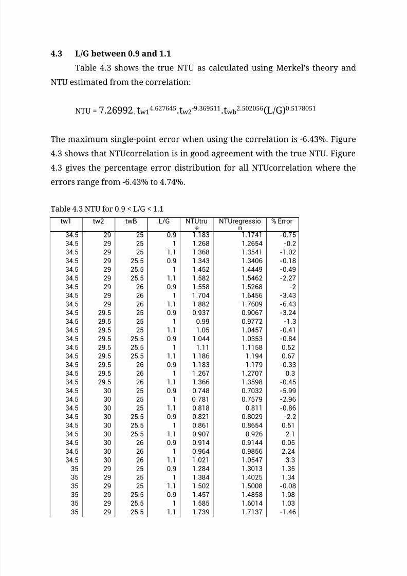
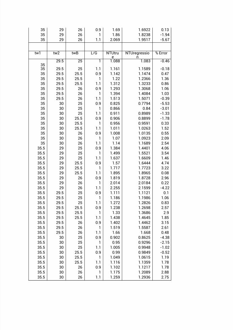
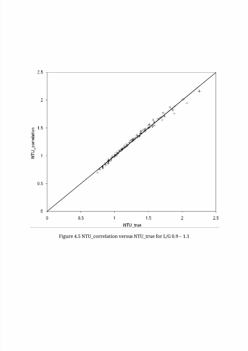
4.3 L/G between 0.9 and 1.1
Table 4.3 shows the true NTU as calculated using Merkel’s theory and
NTU estimated from the correlation:
NTU = 7.26992. tw14.627645.tw2
-9.369511.twb2.502056(L/G)0.5178051
The maximum single-point error when using the correlation is -6.43%. Figure
4.3 shows that NTUcorrelation is in good agreement with the true NTU. Figure
4.3 gives the percentage error distribution for all NTUcorrelation where the
errors range from -6.43% to 4.74%.
Table 4.3 NTU for 0.9 < L/G < 1.1
tw1 tw2 twB L/G NTUtrue
NTUregression
% Error
34.5 29 25 0.9 1.183 1.1741 -0.75
34.5 29 25 1 1.268 1.2654 -0.2
34.5 29 25 1.1 1.368 1.3541 -1.02
34.5 29 25.5 0.9 1.343 1.3406 -0.18
34.5 29 25.5 1 1.452 1.4449 -0.49
34.5 29 25.5 1.1 1.582 1.5462 -2.27
34.5 29 26 0.9 1.558 1.5268 -2
34.5 29 26 1 1.704 1.6456 -3.43
34.5 29 26 1.1 1.882 1.7609 -6.4334.5 29.5 25 0.9 0.937 0.9067 -3.24
34.5 29.5 25 1 0.99 0.9772 -1.3
34.5 29.5 25 1.1 1.05 1.0457 -0.41
34.5 29.5 25.5 0.9 1.044 1.0353 -0.84
34.5 29.5 25.5 1 1.11 1.1158 0.52
34.5 29.5 25.5 1.1 1.186 1.194 0.67
34.5 29.5 26 0.9 1.183 1.179 -0.33
34.5 29.5 26 1 1.267 1.2707 0.3
34.5 29.5 26 1.1 1.366 1.3598 -0.45
34.5 30 25 0.9 0.748 0.7032 -5.99
34.5 30 25 1 0.781 0.7579 -2.96
34.5 30 25 1.1 0.818 0.811 -0.86
34.5 30 25.5 0.9 0.821 0.8029 -2.2
34.5 30 25.5 1 0.861 0.8654 0.51
34.5 30 25.5 1.1 0.907 0.926 2.1
34.5 30 26 0.9 0.914 0.9144 0.05
34.5 30 26 1 0.964 0.9856 2.24
34.5 30 26 1.1 1.021 1.0547 3.3
35 29 25 0.9 1.284 1.3013 1.35
35 29 25 1 1.384 1.4025 1.34
35 29 25 1.1 1.502 1.5008 -0.08
35 29 25.5 0.9 1.457 1.4858 1.98
35 29 25.5 1 1.585 1.6014 1.0335 29 25.5 1.1 1.739 1.7137 -1.46
Page 22
7/17/2019 13_Chapter One - Six
http://slidepdf.com/reader/full/13chapter-one-six 22/34
35 29 26 0.9 1.69 1.6922 0.13
35 29 26 1 1.86 1.8238 -1.94
35 29 26 1.1 2.069 1.9517 -5.67
tw1 tw2 twB L/G NTUtru
e
NTUregressio
n
% Error
3529.5 25 1 1.088 1.083 -0.46
35 29.5 25 1.1 1.161 1.1589 -0.18
35 29.5 25.5 0.9 1.142 1.1474 0.47
35 29.5 25.5 1 1.22 1.2366 1.36
35 29.5 25.5 1.1 1.312 1.3233 0.86
35 29.5 26 0.9 1.293 1.3068 1.06
35 29.5 26 1 1.394 1.4084 1.03
35 29.5 26 1.1 1.513 1.5071 -0.39
35 30 25 0.9 0.825 0.7794 -5.53
35 30 25 1 0.866 0.84 -3.01
35 30 25 1.1 0.911 0.8989 -1.33
35 30 25.5 0.9 0.906 0.8899 -1.78
35 30 25.5 1 0.956 0.9591 0.33
35 30 25.5 1.1 1.011 1.0263 1.52
35 30 26 0.9 1.008 1.0135 0.55
35 30 26 1 1.07 1.0923 2.09
35 30 26 1.1 1.14 1.1689 2.54
35.5 29 25 0.9 1.384 1.4401 4.06
35.5 29 25 1 1.499 1.5521 3.54
35.5 29 25 1.1 1.637 1.6609 1.46
35.5 29 25.5 0.9 1.57 1.6444 4.74
35.5 29 25.5 1 1.717 1.7723 3.22
35.5 29 25.5 1.1 1.895 1.8965 0.0835.5 29 26 0.9 1.819 1.8728 2.96
35.5 29 26 1 2.014 2.0184 0.22
35.5 29 26 1.1 2.255 2.1599 -4.22
35.5 29.5 25 0.9 1.111 1.1121 0.1
35.5 29.5 25 1 1.186 1.1986 1.06
35.5 29.5 25 1.1 1.272 1.2826 0.83
35.5 29.5 25.5 0.9 1.238 1.2698 2.57
35.5 29.5 25.5 1 1.33 1.3686 2.9
35.5 29.5 25.5 1.1 1.438 1.4645 1.85
35.5 29.5 26 0.9 1.402 1.4462 3.15
35.5 29.5 26 1 1.519 1.5587 2.61
35.5 29.5 26 1.1 1.66 1.668 0.4835.5 30 25 0.9 0.902 0.8625 -4.38
35.5 30 25 1 0.95 0.9296 -2.15
35.5 30 25 1.1 1.005 0.9948 -1.02
35.5 30 25.5 0.9 0.99 0.9849 -0.52
35.5 30 25.5 1 1.049 1.0615 1.19
35.5 30 25.5 1.1 1.116 1.1359 1.78
35.5 30 26 0.9 1.102 1.1217 1.78
35.5 30 26 1 1.175 1.2089 2.88
35.5 30 26 1.1 1.259 1.2936 2.75
Page 23
7/17/2019 13_Chapter One - Six
http://slidepdf.com/reader/full/13chapter-one-six 23/34
Figure 4.5 NTU_correlation versus NTU_true for L/G 0.9 – 1.1
Page 24
7/17/2019 13_Chapter One - Six
http://slidepdf.com/reader/full/13chapter-one-six 24/34
Figure 4.6 Percentage error in NTUcorrelation for for L/G 0.9 – 1.1
Page 25
7/17/2019 13_Chapter One - Six
http://slidepdf.com/reader/full/13chapter-one-six 25/34
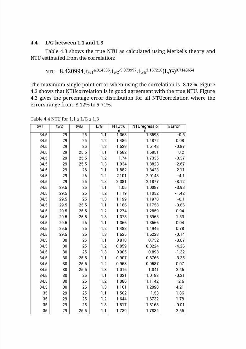
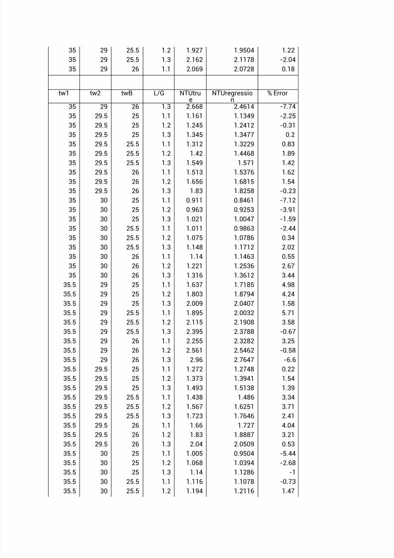
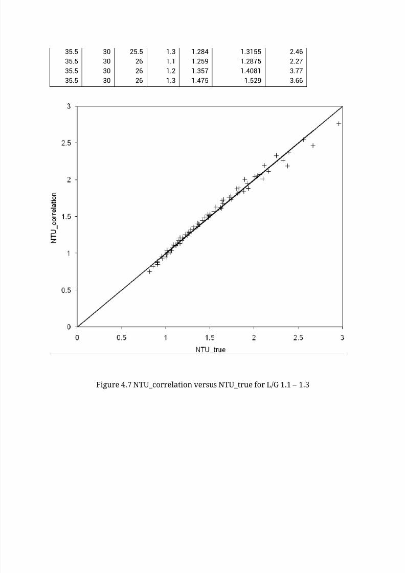
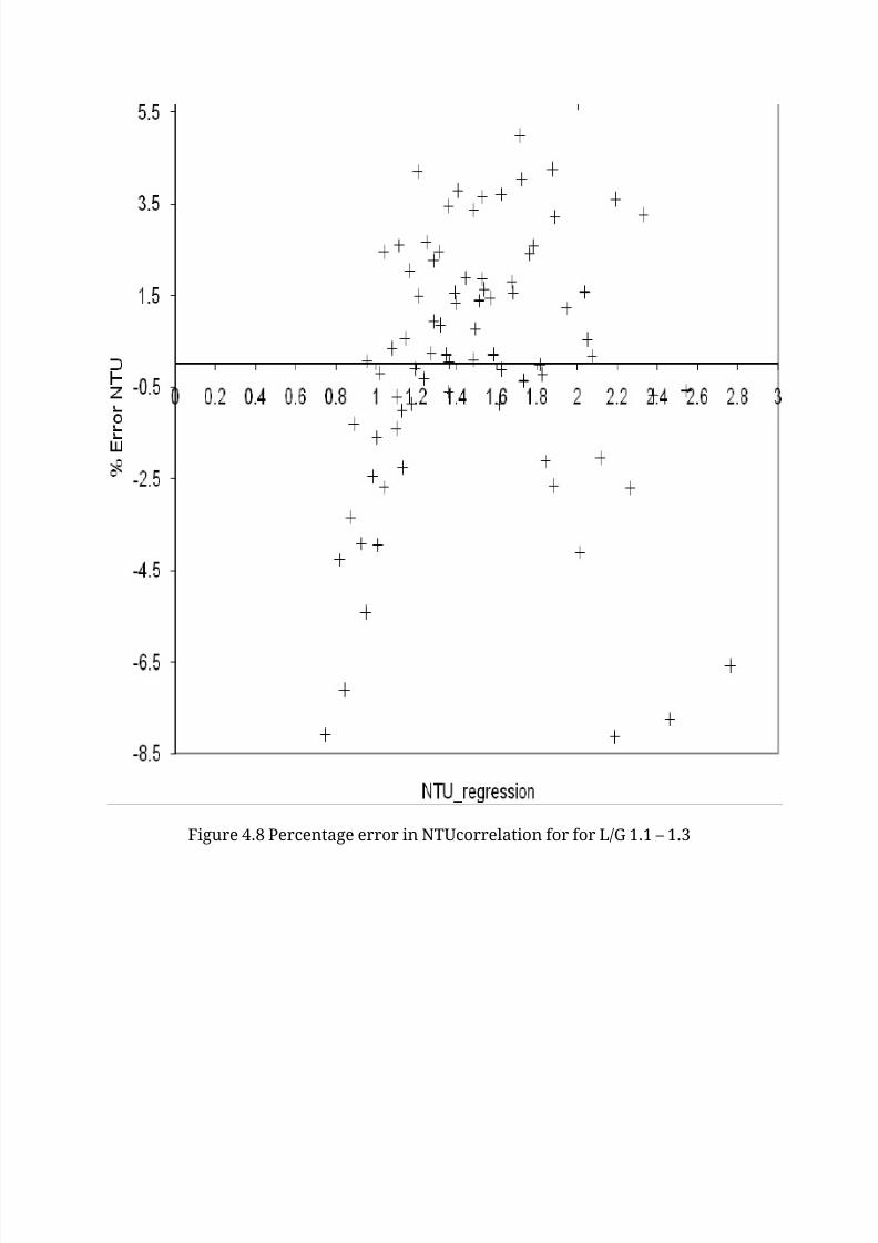
4.4 L/G between 1.1 and 1.3
Table 4.3 shows the true NTU as calculated using Merkel’s theory and
NTU estimated from the correlation:
NTU = 8.420994. tw14.314386.tw2
-9.973997.twb3.167216(L/G)0.7143654
The maximum single-point error when using the correlation is -8.12%. Figure
4.3 shows that NTUcorrelation is in good agreement with the true NTU. Figure
4.3 gives the percentage error distribution for all NTUcorrelation where the
errors range from -8.12% to 5.71%.
Table 4.4 NTU for 1.1 < L/G < 1.3
tw1 tw2 twB L/G NTUtrue
NTUregression
% Error
34.5 29 25 1.1 1.368 1.3598 -0.6
34.5 29 25 1.2 1.486 1.4872 0.08
34.5 29 25 1.3 1.629 1.6148 -0.87
34.5 29 25.5 1.1 1.582 1.5851 0.2
34.5 29 25.5 1.2 1.74 1.7335 -0.37
34.5 29 25.5 1.3 1.934 1.8823 -2.67
34.5 29 26 1.1 1.882 1.8423 -2.11
34.5 29 26 1.2 2.101 2.0148 -4.1
34.5 29 26 1.3 2.381 2.1877 -8.1234.5 29.5 25 1.1 1.05 1.0087 -3.93
34.5 29.5 25 1.2 1.119 1.1032 -1.42
34.5 29.5 25 1.3 1.199 1.1978 -0.1
34.5 29.5 25.5 1.1 1.186 1.1758 -0.86
34.5 29.5 25.5 1.2 1.274 1.2859 0.94
34.5 29.5 25.5 1.3 1.378 1.3963 1.33
34.5 29.5 26 1.1 1.366 1.3666 0.04
34.5 29.5 26 1.2 1.483 1.4945 0.78
34.5 29.5 26 1.3 1.625 1.6228 -0.14
34.5 30 25 1.1 0.818 0.752 -8.07
34.5 30 25 1.2 0.859 0.8224 -4.26
34.5 30 25 1.3 0.905 0.893 -1.32
34.5 30 25.5 1.1 0.907 0.8766 -3.35
34.5 30 25.5 1.2 0.958 0.9587 0.07
34.5 30 25.5 1.3 1.016 1.041 2.46
34.5 30 26 1.1 1.021 1.0188 -0.21
34.5 30 26 1.2 1.086 1.1142 2.6
34.5 30 26 1.3 1.161 1.2098 4.21
35 29 25 1.1 1.502 1.53 1.86
35 29 25 1.2 1.644 1.6732 1.78
35 29 25 1.3 1.817 1.8168 -0.0135 29 25.5 1.1 1.739 1.7834 2.56
Page 26
7/17/2019 13_Chapter One - Six
http://slidepdf.com/reader/full/13chapter-one-six 26/34
35 29 25.5 1.2 1.927 1.9504 1.22
35 29 25.5 1.3 2.162 2.1178 -2.04
35 29 26 1.1 2.069 2.0728 0.18
tw1 tw2 twB L/G NTUtrue
NTUregression
% Error
35 29 26 1.3 2.668 2.4614 -7.74
35 29.5 25 1.1 1.161 1.1349 -2.25
35 29.5 25 1.2 1.245 1.2412 -0.31
35 29.5 25 1.3 1.345 1.3477 0.2
35 29.5 25.5 1.1 1.312 1.3229 0.83
35 29.5 25.5 1.2 1.42 1.4468 1.89
35 29.5 25.5 1.3 1.549 1.571 1.42
35 29.5 26 1.1 1.513 1.5376 1.62
35 29.5 26 1.2 1.656 1.6815 1.54
35 29.5 26 1.3 1.83 1.8258 -0.23
35 30 25 1.1 0.911 0.8461 -7.12
35 30 25 1.2 0.963 0.9253 -3.91
35 30 25 1.3 1.021 1.0047 -1.59
35 30 25.5 1.1 1.011 0.9863 -2.44
35 30 25.5 1.2 1.075 1.0786 0.34
35 30 25.5 1.3 1.148 1.1712 2.02
35 30 26 1.1 1.14 1.1463 0.55
35 30 26 1.2 1.221 1.2536 2.67
35 30 26 1.3 1.316 1.3612 3.44
35.5 29 25 1.1 1.637 1.7185 4.98
35.5 29 25 1.2 1.803 1.8794 4.2435.5 29 25 1.3 2.009 2.0407 1.58
35.5 29 25.5 1.1 1.895 2.0032 5.71
35.5 29 25.5 1.2 2.115 2.1908 3.58
35.5 29 25.5 1.3 2.395 2.3788 -0.67
35.5 29 26 1.1 2.255 2.3282 3.25
35.5 29 26 1.2 2.561 2.5462 -0.58
35.5 29 26 1.3 2.96 2.7647 -6.6
35.5 29.5 25 1.1 1.272 1.2748 0.22
35.5 29.5 25 1.2 1.373 1.3941 1.54
35.5 29.5 25 1.3 1.493 1.5138 1.3935.5 29.5 25.5 1.1 1.438 1.486 3.34
35.5 29.5 25.5 1.2 1.567 1.6251 3.71
35.5 29.5 25.5 1.3 1.723 1.7646 2.41
35.5 29.5 26 1.1 1.66 1.727 4.04
35.5 29.5 26 1.2 1.83 1.8887 3.21
35.5 29.5 26 1.3 2.04 2.0509 0.53
35.5 30 25 1.1 1.005 0.9504 -5.44
35.5 30 25 1.2 1.068 1.0394 -2.68
35.5 30 25 1.3 1.14 1.1286 -1
35.5 30 25.5 1.1 1.116 1.1078 -0.73
35.5 30 25.5 1.2 1.194 1.2116 1.47
Page 27
7/17/2019 13_Chapter One - Six
http://slidepdf.com/reader/full/13chapter-one-six 27/34
35.5 30 25.5 1.3 1.284 1.3155 2.46
35.5 30 26 1.1 1.259 1.2875 2.27
35.5 30 26 1.2 1.357 1.4081 3.77
35.5 30 26 1.3 1.475 1.529 3.66
Figure 4.7 NTU_correlation versus NTU_true for L/G 1.1 – 1.3
Page 28
7/17/2019 13_Chapter One - Six
http://slidepdf.com/reader/full/13chapter-one-six 28/34
Figure 4.8 Percentage error in NTUcorrelation for for L/G 1.1 – 1.3
Page 29
7/17/2019 13_Chapter One - Six
http://slidepdf.com/reader/full/13chapter-one-six 29/34
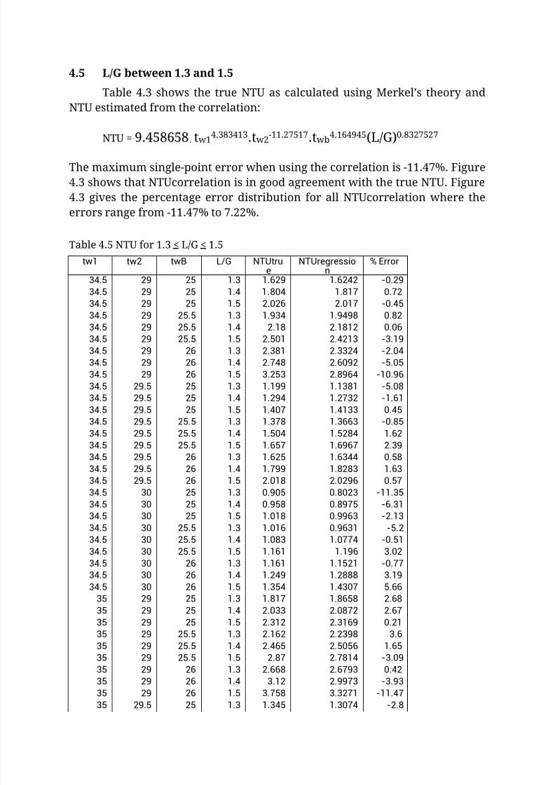
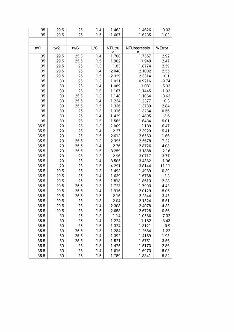
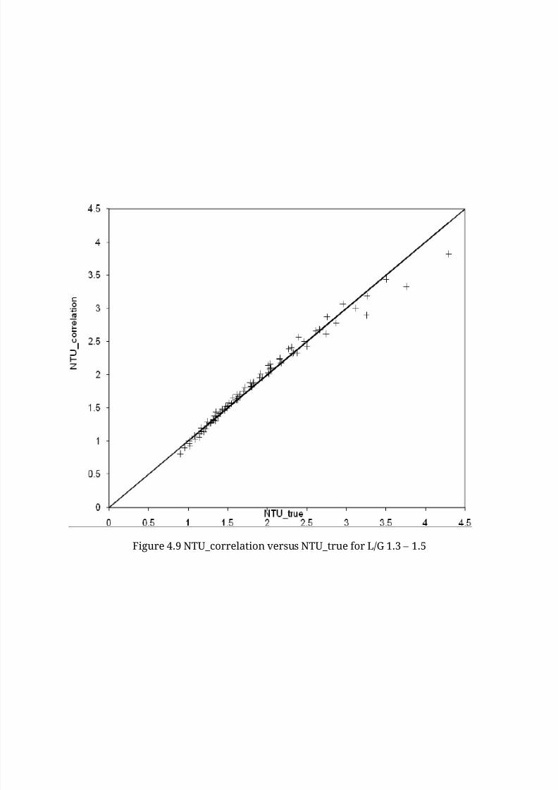
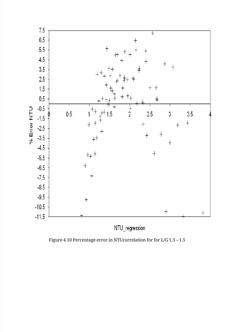
4.5 L/G between 1.3 and 1.5
Table 4.3 shows the true NTU as calculated using Merkel’s theory and
NTU estimated from the correlation:
NTU = 9.458658. tw14.383413.tw2-11.27517.twb4.164945(L/G)0.8327527
The maximum single-point error when using the correlation is -11.47%. Figure
4.3 shows that NTUcorrelation is in good agreement with the true NTU. Figure
4.3 gives the percentage error distribution for all NTUcorrelation where the
errors range from -11.47% to 7.22%.
Table 4.5 NTU for 1.3 < L/G < 1.5
tw1 tw2 twB L/G NTUtru
e
NTUregressio
n
% Error
34.5 29 25 1.3 1.629 1.6242 -0.29
34.5 29 25 1.4 1.804 1.817 0.72
34.5 29 25 1.5 2.026 2.017 -0.45
34.5 29 25.5 1.3 1.934 1.9498 0.82
34.5 29 25.5 1.4 2.18 2.1812 0.06
34.5 29 25.5 1.5 2.501 2.4213 -3.19
34.5 29 26 1.3 2.381 2.3324 -2.04
34.5 29 26 1.4 2.748 2.6092 -5.05
34.5 29 26 1.5 3.253 2.8964 -10.96
34.5 29.5 25 1.3 1.199 1.1381 -5.08
34.5 29.5 25 1.4 1.294 1.2732 -1.61
34.5 29.5 25 1.5 1.407 1.4133 0.4534.5 29.5 25.5 1.3 1.378 1.3663 -0.85
34.5 29.5 25.5 1.4 1.504 1.5284 1.62
34.5 29.5 25.5 1.5 1.657 1.6967 2.39
34.5 29.5 26 1.3 1.625 1.6344 0.58
34.5 29.5 26 1.4 1.799 1.8283 1.63
34.5 29.5 26 1.5 2.018 2.0296 0.57
34.5 30 25 1.3 0.905 0.8023 -11.35
34.5 30 25 1.4 0.958 0.8975 -6.31
34.5 30 25 1.5 1.018 0.9963 -2.13
34.5 30 25.5 1.3 1.016 0.9631 -5.2
34.5 30 25.5 1.4 1.083 1.0774 -0.51
34.5 30 25.5 1.5 1.161 1.196 3.0234.5 30 26 1.3 1.161 1.1521 -0.77
34.5 30 26 1.4 1.249 1.2888 3.19
34.5 30 26 1.5 1.354 1.4307 5.66
35 29 25 1.3 1.817 1.8658 2.68
35 29 25 1.4 2.033 2.0872 2.67
35 29 25 1.5 2.312 2.3169 0.21
35 29 25.5 1.3 2.162 2.2398 3.6
35 29 25.5 1.4 2.465 2.5056 1.65
35 29 25.5 1.5 2.87 2.7814 -3.09
35 29 26 1.3 2.668 2.6793 0.42
35 29 26 1.4 3.12 2.9973 -3.93
35 29 26 1.5 3.758 3.3271 -11.47
35 29.5 25 1.3 1.345 1.3074 -2.8
Page 30
7/17/2019 13_Chapter One - Six
http://slidepdf.com/reader/full/13chapter-one-six 30/34
35 29.5 25 1.4 1.463 1.4626 -0.03
35 29.5 25 1.5 1.607 1.6235 1.03
tw1 tw2 twB L/G NTUtrue
NTUregression
% Error
35 29.5 25.5 1.4 1.706 1.7557 2.9235 29.5 25.5 1.5 1.902 1.949 2.47
35 29.5 26 1.3 1.83 1.8774 2.59
35 29.5 26 1.4 2.048 2.1002 2.55
35 29.5 26 1.5 2.329 2.3314 0.1
35 30 25 1.3 1.021 0.9216 -9.74
35 30 25 1.4 1.089 1.031 -5.33
35 30 25 1.5 1.167 1.1445 -1.93
35 30 25.5 1.3 1.148 1.1064 -3.63
35 30 25.5 1.4 1.234 1.2377 0.3
35 30 25.5 1.5 1.336 1.3739 2.84
35 30 26 1.3 1.316 1.3234 0.56
35 30 26 1.4 1.429 1.4805 3.635 30 26 1.5 1.565 1.6434 5.01
35.5 29 25 1.3 2.009 2.139 6.47
35.5 29 25 1.4 2.27 2.3929 5.41
35.5 29 25 1.5 2.613 2.6563 1.66
35.5 29 25.5 1.3 2.395 2.5678 7.22
35.5 29 25.5 1.4 2.76 2.8726 4.08
35.5 29 25.5 1.5 3.259 3.1888 -2.16
35.5 29 26 1.3 2.96 3.0717 3.77
35.5 29 26 1.4 3.505 3.4362 -1.96
35.5 29 26 1.5 4.291 3.8144 -11.11
35.5 29.5 25 1.3 1.493 1.4989 0.39
35.5 29.5 25 1.4 1.639 1.6768 2.335.5 29.5 25 1.5 1.818 1.8613 2.38
35.5 29.5 25.5 1.3 1.723 1.7993 4.43
35.5 29.5 25.5 1.4 1.916 2.0129 5.06
35.5 29.5 25.5 1.5 2.16 2.2344 3.45
35.5 29.5 26 1.3 2.04 2.1524 5.51
35.5 29.5 26 1.4 2.308 2.4078 4.33
35.5 29.5 26 1.5 2.658 2.6728 0.56
35.5 30 25 1.3 1.14 1.0566 -7.32
35.5 30 25 1.4 1.224 1.182 -3.43
35.5 30 25 1.5 1.324 1.3121 -0.9
35.5 30 25.5 1.3 1.284 1.2684 -1.2235.5 30 25.5 1.4 1.392 1.4189 1.93
35.5 30 25.5 1.5 1.521 1.5751 3.56
35.5 30 26 1.3 1.475 1.5173 2.86
35.5 30 26 1.4 1.616 1.6973 5.03
35.5 30 26 1.5 1.789 1.8841 5.32
Page 31
7/17/2019 13_Chapter One - Six
http://slidepdf.com/reader/full/13chapter-one-six 31/34
Figure 4.9 NTU_correlation versus NTU_true for L/G 1.3 – 1.5
Page 32
7/17/2019 13_Chapter One - Six
http://slidepdf.com/reader/full/13chapter-one-six 32/34
Figure 4.10 Percentage error in NTUcorrelation for for L/G 1.3 – 1.5
Page 33
7/17/2019 13_Chapter One - Six
http://slidepdf.com/reader/full/13chapter-one-six 33/34
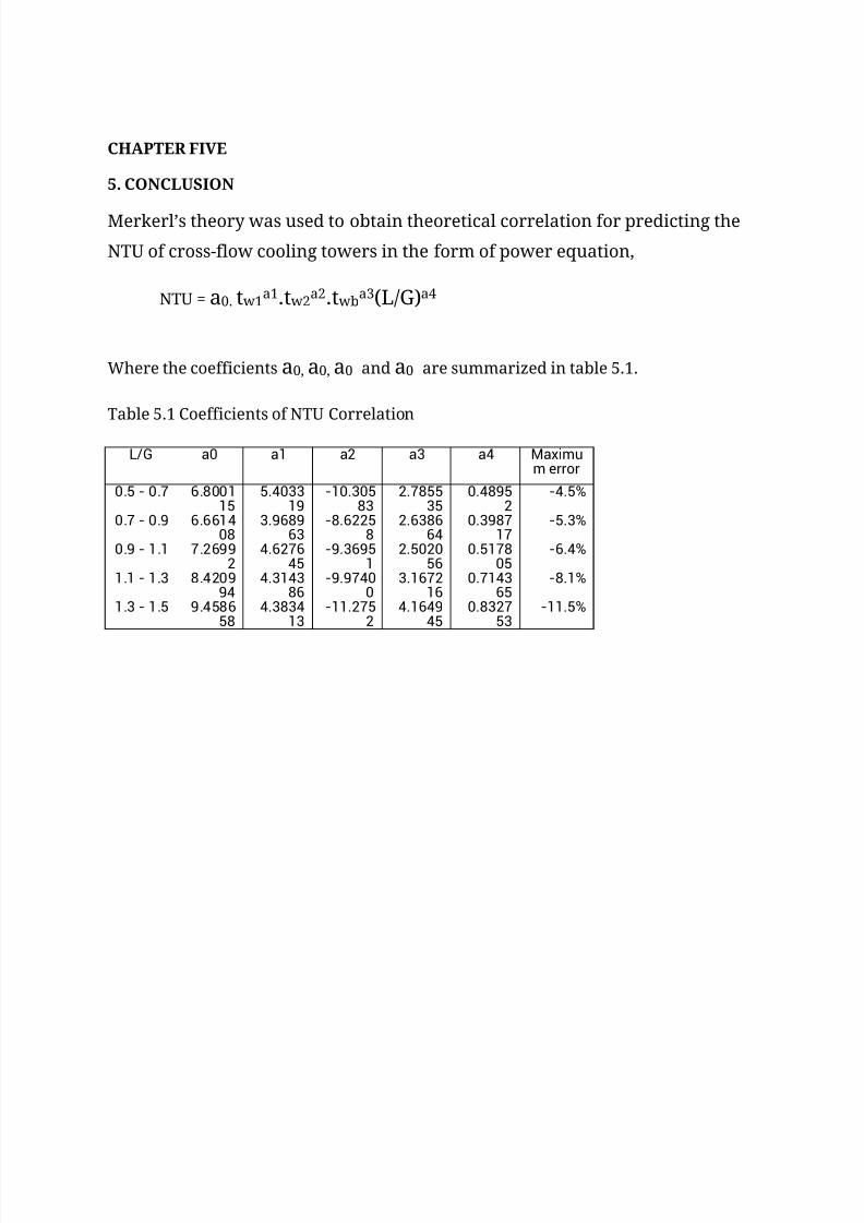
CHAPTER FIVE
5. CONCLUSION
Merkerl’s theory was used to obtain theoretical correlation for predicting the
NTU of cross-flow cooling towers in the form of power equation,
NTU = a0. tw1a1.tw2
a2.twba3(L/G)a4
Where the coefficients a0, a0, a0 and a0 are summarized in table 5.1.
Table 5.1 Coefficients of NTU Correlation
L/G a0 a1 a2 a3 a4 Maximum error
0.5 - 0.7 6.800115
5.403319
-10.30583
2.785535
0.48952
-4.5%
0.7 - 0.9 6.661408
3.968963
-8.62258
2.638664
0.398717
-5.3%
0.9 - 1.1 7.26992
4.627645
-9.36951
2.502056
0.517805
-6.4%
1.1 - 1.3 8.420994
4.314386
-9.97400
3.167216
0.714365
-8.1%
1.3 - 1.5 9.458658
4.383413
-11.2752
4.164945
0.832753
-11.5%
Page 34
7/17/2019 13_Chapter One - Six
http://slidepdf.com/reader/full/13chapter-one-six 34/34
REFERENCES
1.W.F.Stoecker & J.W.Jones, Refrigeration and Air Conditioning Second Edition,McGraw-Hill
2.Dickey, J. B., Evaporative Cooling Towers, Marley Cooling Towers Co., 1978.
3. ASHRAE, “Cooling Towers,” in ASHRAE Handbook—HVAC Systems and Equipment, New York: ASHRAE, 2004.
4. Wistrom, G., “Cold Weather Operation of Crossflow Cooling Towers,” Plant Engineering, September 8, 1975.
5. Lipták, B. G. (ed.), “Cooling Towers: Their Design and Application,” in Environmental Engineer’s Handbook, Lewis Publishers, 1997.
6.Optimal Design of Cooling Towers, Heat and Mass Transfer - Modeling andSimulation, Prof. Md Monwar Hossain (Ed.), ISBN: 978-953-307-604-1, InTech,Available from: http://www.intechopen.com/books/heat-andmass-transfer-modeling-and-simulation/optimal-design-of-cooling-towers