14.581 International Trade Š Lecture 1 Š Comparative ... · 14.581 International Trade Š Lecture...

14.581 International Trade Lecture 1

Comparative Advantage and Gains from Trade

14.581

Week 1

Spring 2013

14.581 (Week 1) CA and GT Spring 2013 1 / 31

Todays Plan

1 Course logistics2 A Brief History of the Field3 Neoclassical Trade: Standard Assumptions4 Neoclassical Trade: General Results

1 Gains from Trade2 Law of Comparative Advantage


Course Logistics

Recitations: TBA

No required textbooks, but we will frequently use:

Dixit and Norman, Theory of International Trade (DN)Feenstra, Advanced International Trade: Theory and Evidence (F)Helpman and Krugman, Market Structure and Foreign Trade (HKa)

Relevant chapters of all textbooks will be available on Stellar


Course Logistics

Course requirements:

Four problem sets: 50% of the course gradeOne referee report: 15% of the course gradeOne research proposal: 35% of the course grade


Course Logistics

Course outline:1 Ricardian and Assignment Models (4 weeks)2 Factor Proportion Theory (2 weeks)3 Firm Heterogeneity Models (2 weeks)4 Gravity Models (1 week)5 Topics:

1 Economic Geography (1 week)2 O¤shoring (1 week)3 Trade Policy (2 weeks)


A Brief History of the FieldTwo hundred years of theory

1 1830-1980: Neoclassical trade theory) Ricardo) Heckscher-Ohlin-Samuelson) Dixit-Norman

2 1980-1990: New trade theory) Krugman-Helpman) Brander-Krugman) Grossman-Helpman


A Brief History of the FieldThe discovery of trade data

1 1990-2000: Empirical trade) Leamer, Treer, Davis-Weinstein) Bernard, Tybout

2 2000-2010: Firm-level heterogeneity) Melitz) Eaton-Kortum

3 Where are we now?


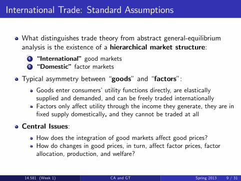
International Trade: Standard Assumptions

What distinguishes trade theory from abstract general-equilibriumanalysis is the existence of a hierarchical market structure:

1 International good markets2 Domestic factor markets

Typical asymmetry between goodsand factors:

Goods enter consumersutility functions directly, are elasticallysupplied and demanded, and can be freely traded internationallyFactors only a¤ect utility through the income they generate, they are inxed supply domestically, and they cannot be traded at all

Central Issues:

How does the integration of good markets a¤ect good prices?How do changes in good prices, in turn, a¤ect factor prices, factorallocation, production, and welfare?


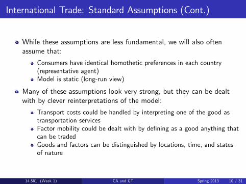
International Trade: Standard Assumptions (Cont.)

While these assumptions are less fundamental, we will also oftenassume that:

Consumers have identical homothetic preferences in each country(representative agent)Model is static (long-run view)

Many of these assumptions look very strong, but they can be dealtwith by clever reinterpretations of the model:

Transport costs could be handled by interpreting one of the good astransportation servicesFactor mobility could be dealt with by dening as a good anything thatcan be tradedGoods and factors can be distinguished by locations, time, and statesof nature


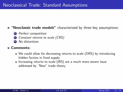
Neoclassical Trade: Standard Assumptions

Neoclassic trade models characterized by three key assumptions:1 Perfect competition2 Constant returns to scale (CRS)3 No distortions

Comments:

We could allow for decreasing returns to scale (DRS) by introducinghidden factors in xed supplyIncreasing returns to scale (IRS) are a much more severe issueaddressed by New trade theory


Neoclassical Trade: General Results

Not surprisingly, there are few results that can be derived using onlyAssumptions 1-3

In future lectures, we will derive sharp predictions for special cases:Ricardo, Assignment, Ricardo-Viner, and Heckscher-Ohlin models

Today, well stick to the general case and show how simple revealedpreference arguments can be used to establish two important results:

1 Gains from trade (Samuelson 1939)2 Law of comparative advantage (Deardor¤ 1980)


Basic Environment

Consider a world economy with n = 1, ...,N countries, each populatedby h = 1, ...,Hn households

There are g = 1, ...,G goods:

yn (yn1 , ..., ynG ) Output vector in country ncnh (cnh1 , ..., cnhG ) Consumption vector of household h in country npn (pn1 , ..., pnG ) Good price vector in country n

There are f = 1, ...,F factors:

vn (vn1 , ..., vnF ) Endowment vector in country nwn (wn1 , ...,wnF ) Factor price vector in country n


SupplyThe revenue function

We denote by Ωn the set of combinations (y , v) feasible in country n

CRS ) Ωn is a convex cone

Revenue function in country n is dened as

rn(p, v) maxyfpy j(y , v) 2 Ωng

Comments (see Dixit-Norman pp. 31-36 for details):

Revenue function summarizes all relevant properties of technologyUnder perfect competition, yn maximizes the value of output incountry n:

rn(pn , vn) = pnyn (1)


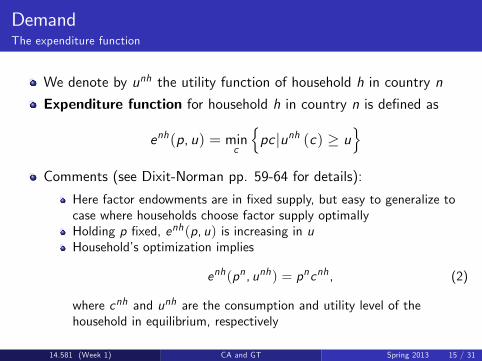
DemandThe expenditure function

We denote by unh the utility function of household h in country n

Expenditure function for household h in country n is dened as

enh(p, u) = minc

npc junh (c) u

oComments (see Dixit-Norman pp. 59-64 for details):

Here factor endowments are in xed supply, but easy to generalize tocase where households choose factor supply optimallyHolding p xed, enh(p, u) is increasing in uHouseholds optimization implies

enh(pn , unh) = pncnh , (2)

where cnh and unh are the consumption and utility level of thehousehold in equilibrium, respectively


Gains from TradeOne household per country

In the next propositions, when we say in a neoclassical trade model,we mean in a model where equations (1) and (2) hold in anyequilibrium

Consider rst the case where there is just one household per country

Without risk of confusion, we drop h and n from all variables

Instead we denote by:

(ya, ca, pa) the vector of output, consumption, and good prices underautarky(y , c , p) the vector of output, consumption, and good prices under freetradeua and u the utility levels under autarky and free trade



Proposition 1 In a neoclassical trade model with one household percountry, free trade makes all households (weakly) better o¤.

Proof:

e(p, ua) pca, by denition of e= py a by market clearing under autarky r (p, v) by denition of r= e (p, u) by equations (1), (2), and trade balance

Since e(p, ) increasing, we get u ua



Comments:

Two inequalities in the previous proof correspond to consumption andproduction gains from tradePrevious inequalities are weak. Equality if kinks in IC or PPFPrevious proposition only establishes that households always preferfree trade to autarky. It does not say anything about thecomparisons of trade equilibria


Gains from TradeMultiple households per country (I): domestic lump-sum transfers

With multiple-households, moving away from autarky is likely tocreate winners and losers

How does that relate to the previous comment?

In order to establish the Pareto-superiority of trade, we will thereforeneed to allow for policy instruments. We start with domesticlump-sum transfers and then consider

We now reintroduce the index h explicitly and denote by:

cah and ch the vector of consumption of household h under autarkyand free tradevah and vh the vector of endowments of household h under autarkyand free tradeuah and uh the utility levels of household h under autarky and freetradeτh the lump-sum transfer from the government to household h (τh 0, lump-sum tax and τh 0 , lump-sum subsidy)



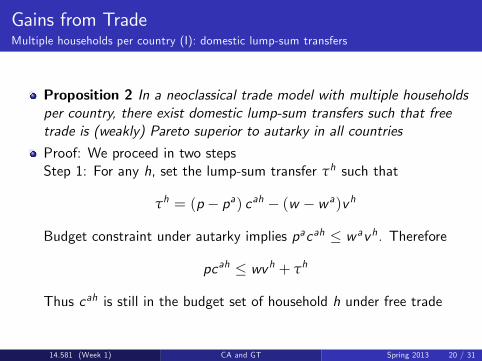
Proposition 2 In a neoclassical trade model with multiple householdsper country, there exist domestic lump-sum transfers such that freetrade is (weakly) Pareto superior to autarky in all countries

Proof: We proceed in two stepsStep 1: For any h, set the lump-sum transfer τh such that

τh = (p pa) cah (w w a)vh

Budget constraint under autarky implies pacah w avh. Therefore

pcah wvh + τh

Thus cah is still in the budget set of household h under free trade



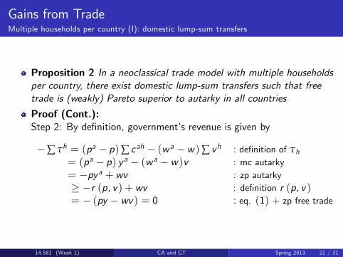
Proposition 2 In a neoclassical trade model with multiple householdsper country, there exist domestic lump-sum transfers such that freetrade is (weakly) Pareto superior to autarky in all countries

Proof (Cont.):Step 2: By denition, governments revenue is given by

∑ τh = (pa p)∑ cah (w a w)∑ vh : denition of τh= (pa p) y a (w a w)v : mc autarky= py a + wv : zp autarky r (p, v) + wv : denition r (p, v)= (py wv) = 0 : eq. (1) + zp free trade



Comments:

Good to know we dont need international lump-sum transfersDomestic lump-sum transfers remain informationally intensive (cah?)


Gains from TradeMultiple households per country (II): commodity and factor taxation

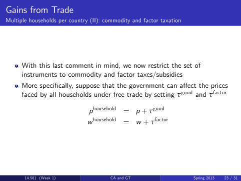
With this last comment in mind, we now restrict the set ofinstruments to commodity and factor taxes/subsidies

More specically, suppose that the government can a¤ect the pricesfaced by all households under free trade by setting τgood and τfactor

phousehold = p + τgood

whousehold = w + τfactor



Proposition 3 In a neoclassical trade model with multiple householdsper country, there exist commodity and factor taxes/subsidies suchthat free trade is (weakly) Pareto superior to autarky in all countries

Proof: Consider the two following taxes:

τgood = pa pτfactor = w a w

By construction, household is indi¤erent between autarky and freetrade. Now consider governments revenues. By denition

∑ τh = τgood ∑ cah τfactor ∑ vh

= (pa p)∑ cah (w a w)∑ vh 0,

for the same reason as in the previous proof.



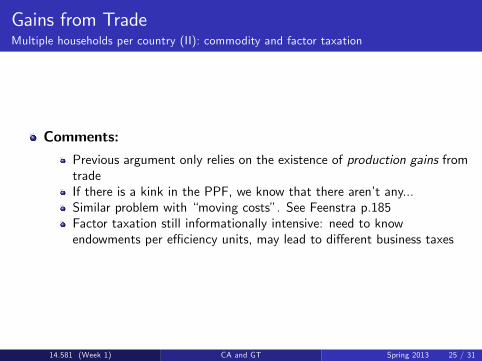
Comments:

Previous argument only relies on the existence of production gains fromtradeIf there is a kink in the PPF, we know that there arent any...Similar problem with moving costs. See Feenstra p.185Factor taxation still informationally intensive: need to knowendowments per e¢ ciency units, may lead to di¤erent business taxes


Law of Comparative AdvantageBasic Idea

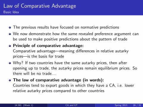
The previous results have focused on normative predictions

We now demonstrate how the same revealed preference argument canbe used to make positive predictions about the pattern of trade

Principle of comparative advantage:Comparative advantage meaning di¤erences in relative autarkyprices is the basis for trade

Why? If two countries have the same autarky prices, then afteropening up to trade, the autarky prices remain equilibrium prices. Sothere will be no trade....

The law of comparative advantage (in words):Countries tend to export goods in which they have a CA, i.e. lowerrelative autarky prices compared to other countries


Law of Comparative AdvantageDixit-Norman-Deardor¤ (1980)

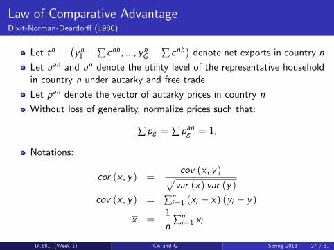
Let tn yn1 ∑ cnh, ..., ynG ∑ cnh

denote net exports in country n

Let uan and un denote the utility level of the representative householdin country n under autarky and free trade

Let pan denote the vector of autarky prices in country n

Without loss of generality, normalize prices such that:

∑ pg = ∑ pang = 1,

Notations:

cor (x , y) =cov (x , y)pvar (x) var (y)

cov (x , y) = ∑ni=1 (xi x) (yi y)

x =1n

∑ni=1 xi



Proposition 4 In a neoclassical trade model, if there is arepresentative household in country n, then cor (p pa, tn) 0Proof: Since (yn, vn) 2 Ωn, the denition of r implies

payn r (pa, vn)

Since un (cn) = un, the denition of e implies

pacn e (pa, un)

The two previous inequalities imply

patn r (pa, vn) e (pa, un) (3)

Since un uan by Proposition 1, e (pa, ) increasing implies

e(pa, un) e(pa, una) (4)



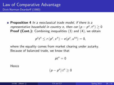
Proposition 4 In a neoclassical trade model, if there is arepresentative household in country n, then cor (p pa, tn) 0Proof (Cont.): Combining inequalities (3) and (4), we obtain

patn r (pa, vn) e(pa, una) = 0,

where the equality comes from market clearing under autarky.Because of balanced trade, we know that

ptn = 0

Hence(p pa) tn 0



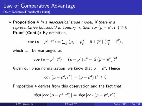
Proposition 4 In a neoclassical trade model, if there is arepresentative household in country n, then cor (p pa, tn) 0Proof (Cont.): By denition,

cov (p pa, tn) = ∑gpg pag p + pa

tng t

n ,which can be rearranged as

cov (p pa, tn) = (p pa) tn G (p pa) tn

Given our price normalization, we know that p = pa. Hence

cov (p pa, tn) = (p pa) tn 0

Proposition 4 derives from this observation and the fact that

sign [cor (p pa, tn)] = sign [cov (p pa, tn)]



Comments:

With 2 goods, each country exports the good in which it has a CA, butwith more goods, this is just a correlationCore of the proof is the observation that patn 0It directly derives from the fact that there are gains from trade. Sincefree trade is better than autarky, the vector of consumptions must beat most barely attainable under autarky (payn pacn)For empirical purposes, problem is that we rarely observe autarky...In future lectures, we will look at models which relate pa to(observable) primitives of the model: technology and factorendowments


MIT OpenCourseWarehttp://ocw.mit.edu

14.581 International Economics ISpring 2013

For information about citing these materials or our Terms of Use, visit: http://ocw.mit.edu/terms.

http://ocw.mit.edu

http://ocw.mit.edu/terms.

Date post:	28-Jun-2018
Category:	Documents
Upload:	trinhlien
View:	226 times
Download:	0 times

14.581 International Trade Š Lecture 1 Š Comparative ... · 14.581 International Trade Š Lecture...

Documents