47
15. Circuits and magnetic field Topics: • Course philosophy • RC circuit • Magnetic field

15. Circuits and magnetic field
Topics:
• Course philosophy
• RC circuit
• Magnetic field

Class attendance helps! Why?
Because class participation and engagement helps
Proof:
Gain is 27% (post-pre)/pre for in-class participation and engagement
Gain is 11% (post-pre/pre for non-class participation and engagement
(source: E. Mazur, 2006)
Gain is 24% in 2017 clicker participation. (The final grade was 24% higher for
those students who participated in all classes, i.e., A vs C+).

Normalized participation (+ epsilon)
Norm
aliz
ed f
inal exam
(+
epsilo
n) Class of 2017

Class attendance helps! Why?
Because class participation and engagement helps
Proof:
Gain is 27% (post-pre)/pre for in-class participation and engagement
Gain is 11% (post-pre/pre for non-class participation and engagement
(source: E. Mazur, 2006)
Gain is 24% in 2017 clicker participation. (The final grade was 24% higher for
those students who participated in all classes, i.e., A vs C+).
Goal: increase class participation and engagement
How: encourage participation and engagement – but also reduce distraction
Those who distract other students in class will be asked to leave. If you
watch Netflix, you will be asked to leave. If you prefer to stay home or not
listen it’s your choice. You can still get your clicker points by connecting to
session ID phys142 during class time. If you only come to class because of
your clicker participation, don’t.
Math: Some of the math we use is advanced (e.g. surface integral for Gauss’s
law). Don’t let this scare you. We always give the recipe of how to solve them in
the simple examples used in this course (we only consider simple geometries,
like spheres, cubes, and cylinders).
If you feel you want more of something, like a more in depth methodology of how
to solve surface integrals, let us know and we can arrange, for example, a tutorial
sessions on topics of your choice. I welcome initiatives.

Demos: Sometimes there will be demos in class to illustrate a concept. Physics
is an experimental science (it is not math) and seeing an experiment can be very
illuminating. Most discoveries in physics were experimental. However, some
demos can take a few minutes, or not always work as planned (even when
testing them five minutes before). I ask for your patience when this happens. I do
my best to minimize the delay.

RC Circuits
In direct current circuits containing capacitors, the current may vary with time.
▪ The current is still in the same direction.
An RC circuit will contain a series combination of a resistor and a capacitor.
Section 28.4
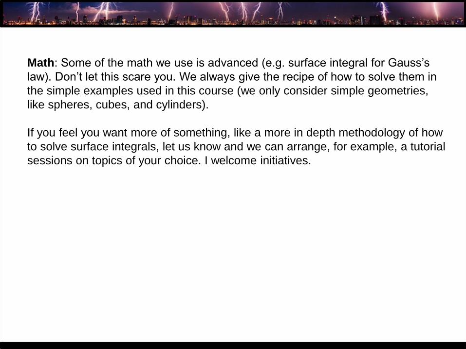
RC Circuit, Example
Section 28.4

RC Circuit, Example
Section 28.4
Volta
ge a
cro
ss t
he c
apacitor In-class experiment
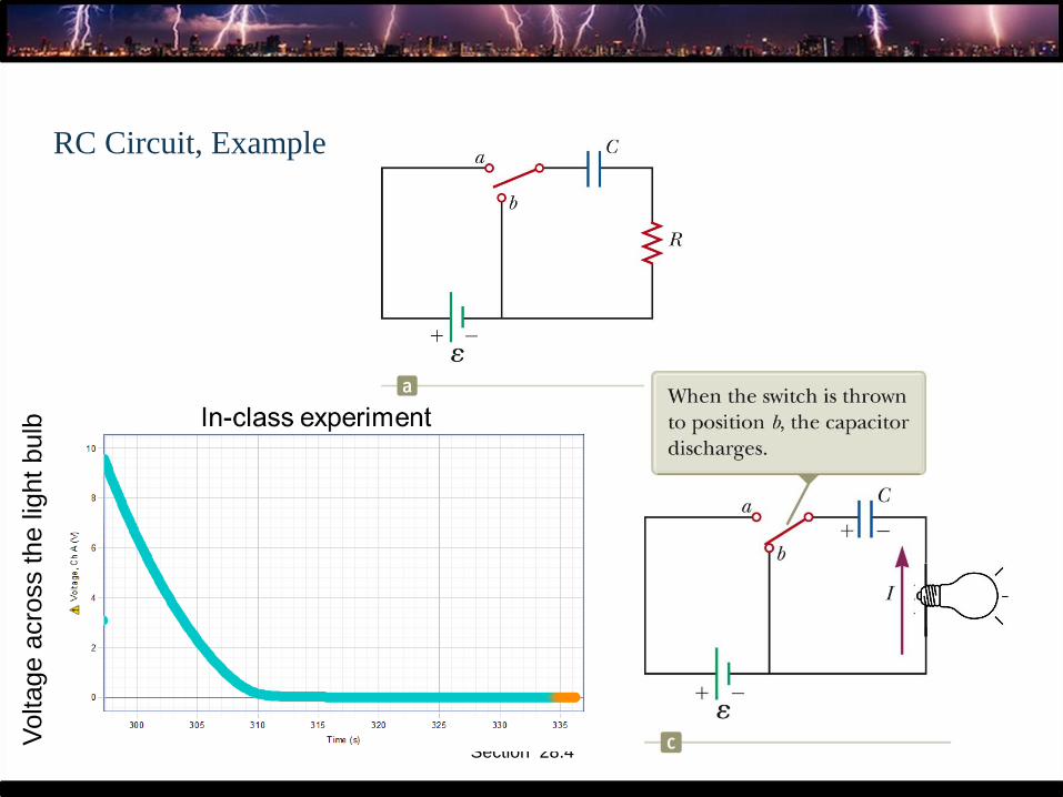
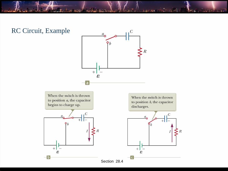
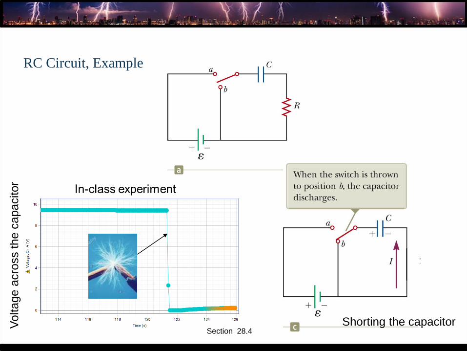
RC Circuit, Example
Section 28.4
Voltage a
cro
ss t
he lig
ht
bulb
RC Circuit, Example
Section 28.4
Voltage a
cro
ss t
he c
apacitor
Shorting the capacitor
Charging a Capacitor
When the circuit is completed, the capacitor starts to charge.
The capacitor continues to charge until it reaches its maximum charge (Q = Cε).
Once the capacitor is fully charged, the current in the circuit is zero.
As the plates are being charged, the potential difference across the capacitor increases.
At the instant the switch is closed, the charge on the capacitor is zero.
Once the maximum charge is reached, the current in the circuit is zero.
▪ The potential difference across the capacitor matches that supplied by the battery.
Section 28.4

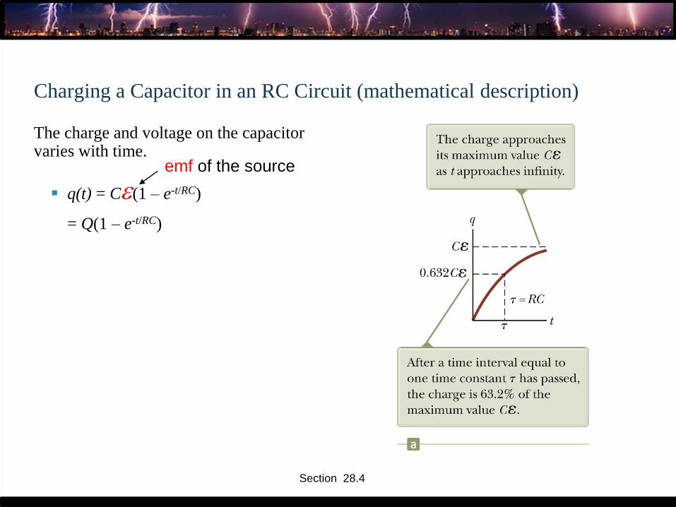
Charging a Capacitor in an RC Circuit (mathematical description)
The charge and voltage on the capacitor varies with time.
Section 28.4
Charging a Capacitor in an RC Circuit (mathematical description)
The charge and voltage on the capacitor varies with time.
▪ q(t) = Ce(1 – e-t/RC)
= Q(1 – e-t/RC)
Section 28.4
emf of the source

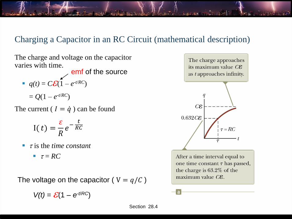
Charging a Capacitor in an RC Circuit (mathematical description)
The charge and voltage on the capacitor varies with time.
▪ q(t) = Ce(1 – e-t/RC)
= Q(1 – e-t/RC)
The current ( 𝐼 = ሶ𝑞 ) can be found
I( 𝑡) =𝜀
𝑅𝑒−
𝑡𝑅𝐶
Section 28.4
emf of the source

Charging a Capacitor in an RC Circuit (mathematical description)
The charge and voltage on the capacitor varies with time.
▪ q(t) = Ce(1 – e-t/RC)
= Q(1 – e-t/RC)
The current ( 𝐼 = ሶ𝑞 ) can be found
▪ t is the time constant
▪ t = RC
I( 𝑡) =𝜀
𝑅𝑒−
𝑡𝑅𝐶
Section 28.4
emf of the source
Charging a Capacitor in an RC Circuit (mathematical description)
The charge and voltage on the capacitor varies with time.
▪ q(t) = Ce(1 – e-t/RC)
= Q(1 – e-t/RC)
The current ( 𝐼 = ሶ𝑞 ) can be found
▪ t is the time constant
▪ t = RC
I( 𝑡) =𝜀
𝑅𝑒−
𝑡𝑅𝐶
Section 28.4
The voltage on the capacitor ( V = 𝑞/𝐶 )
emf of the source
V(t) = e(1 – e-t/RC)

Discharging a Capacitor in an RC Circuit (mathematical description)
When a charged capacitor is placed in the circuit, it can be discharged.
▪ q(t) = Qe-t/RC
The charge decreases exponentially.
Section 28.4

Discharging Capacitor (mathematical description)
At t = t = RC, the charge decreases to 0.368 Qmax
▪ In other words, in one time constant, the capacitor loses 63.2% of its initial charge.
The current can be found
Both charge and current decay exponentially at a rate characterized by t = RC.
( )I t RCdq Qt e
dt RC
−= = −
Section 28.4
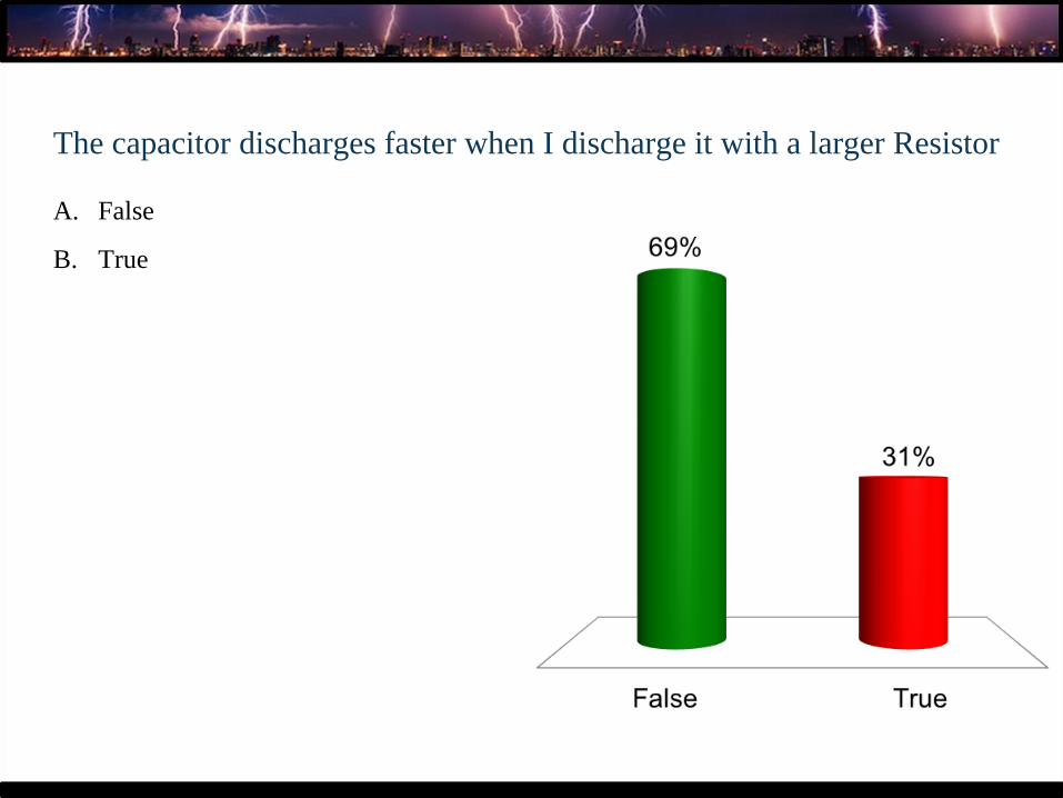
The capacitor discharges faster when I discharge it with a larger Resistor
A. False
B. True

Kirchhoff’s Rules
There are ways in which resistors can be connected so that the circuits formed cannot be
reduced to a single equivalent resistor.
Two rules, called Kirchhoff’s rules, can be used instead.
Section 28.3
0junction
I =(1) (junction rule)I1 - I2 - I3 = 0
closedloop
0V =(2) (loop rule)

Examples of resistances and Kirchhoff:
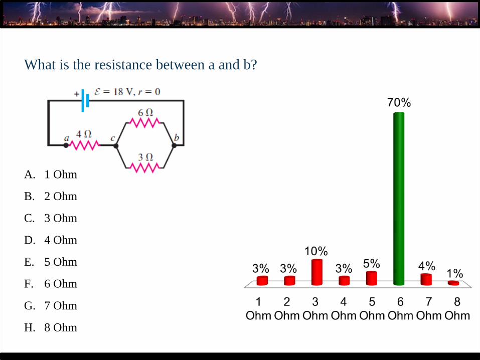
What is the resistance between a and b?
A. 1 Ohm
B. 2 Ohm
C. 3 Ohm
D. 4 Ohm
E. 5 Ohm
F. 6 Ohm
G. 7 Ohm
H. 8 Ohm

Associated concepts:

What is the current at c?
A. 2 A towards the right
B. 2 A towards the left
C. 1 A towards the right
D. 1 A towards the left
c

Associated concepts:
0junction
I =(1) (junction rule)

1 AAt junction a: 1+1-2=0 c
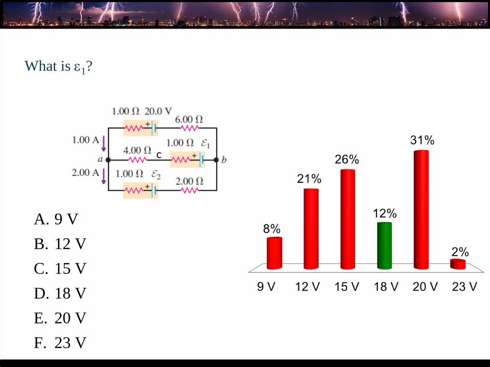
What is e1?
A. 9 V
B. 12 V
C. 15 V
D. 18 V
E. 20 V
F. 23 V
c

20-1+4+1-e1-6=0=>e1=18VGreen loop:
c
closedloop
0V =(2) (loop rule)

What is e2?
A. 5 V
B. 7 V
C. 12 V
D. 18 V
E. 20 V
F. 23 V
c

20-1-2-e2-4-6=0=>e2=7V
c
closedloop
0V =(2) (loop rule)

20-1-2-e2-4-6=0=>e2=7V20-1+4+1-e1-6=0=>e1=18Ve1-1-4-2-e2-4=0=>e1=e2+11
c
closedloop
0V =(2) (loop rule)

What is the power through the 18 Ohm resistor?
A. 34.7 W
B. 107 W
C. 13.1 W
D. 67.2 W

Power:
Associated concepts:

I
I1
I2
Rtot=1/(1/45+1/15)+18 => I=25/Rtot=0.85 A
Using parallel resistors:
P=18*I^2=13.1 W
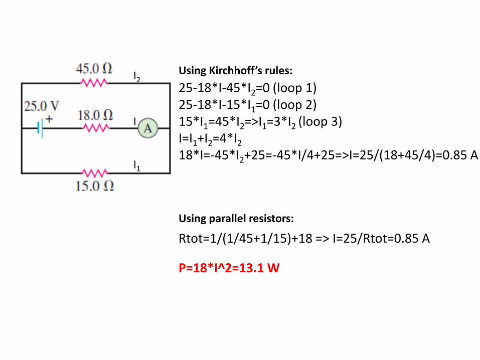
25-18*I-45*I2=0 (loop 1)25-18*I-15*I1=0 (loop 2)15*I1=45*I2=>I1=3*I2 (loop 3)I=I1+I2=4*I2
18*I=-45*I2+25=-45*I/4+25=>I=25/(18+45/4)=0.85 A
I
I1
I2
Rtot=1/(1/45+1/15)+18 => I=25/Rtot=0.85 A
Using Kirchhoff’s rules:
Using parallel resistors:
P=18*I^2=13.1 W

Magnetic fields

Magnetic Field Lines, Bar Magnet Example
The compass can be used to trace the field
lines.
The lines outside the magnet point from the
North pole to the South pole.
Section 29.1


Magnetic Field Lines, Bar Magnet
Iron filings are used to show the pattern of
the electric field lines.
The direction of the field is the direction a
north pole would point.
Section 29.1

Magnetic Field Lines, Opposite Poles
Iron filings are used to show the pattern of
the electric field lines.
The direction of the field is the direction a
north pole would point.
▪ Compare to the electric field produced
by an electric dipole
Section 29.1

Magnetic Field Lines, Like Poles
Iron filings are used to show the pattern of
the electric field lines.
The direction of the field is the direction a
north pole would point.
▪ Compare to the electric field produced
by like charges
Section 29.1

Earth’s Magnetic Poles
More proper terminology would be that a magnet has “north-seeking” and “south-
seeking” poles.
The north-seeking pole points to the north geographic pole.
▪ This would correspond to the Earth’s south magnetic pole.
The south-seeking pole points to the south geographic pole.
▪ This would correspond to the Earth’s north magnetic pole.
The configuration of the Earth’s magnetic field is very much like the one that would be
achieved by burying a gigantic bar magnet deep in the Earth’s interior.
Section 29.1

Earth’s Magnetic Field
The source of the Earth’s magnetic field is
likely convection currents in the Earth’s
core.
There is strong evidence that the magnitude
of a planet’s magnetic field is related to its
rate of rotation.
The direction of the Earth’s magnetic field
reverses periodically.
Section 29.1

𝑞 Ԧ𝑣 × 𝐵 = Ԧ𝐹
v: Towards velocity (Thumbs) × Magnetic field (Middle finger) = Force (slap)
Ԧ𝐹
Ԧ𝑣
𝐵
(1) Magnetic force:
Right hand; positive charge
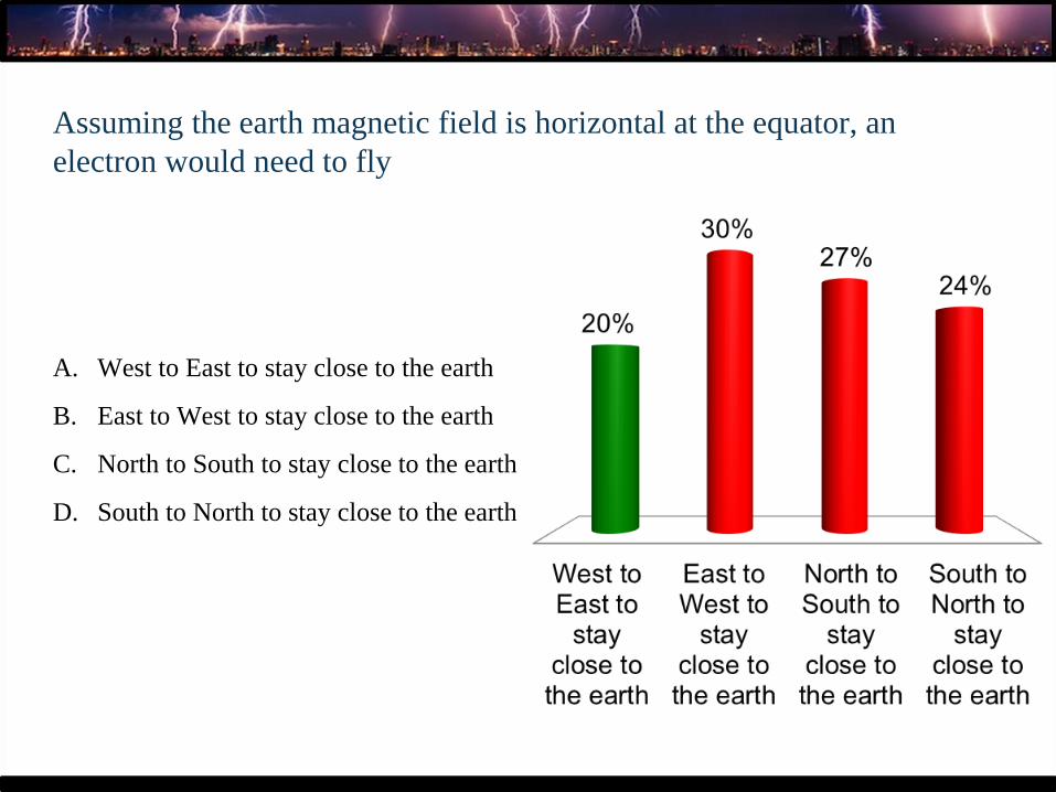
Assuming the earth magnetic field is horizontal at the equator, an
electron would need to fly
A. West to East to stay close to the earth
B. East to West to stay close to the earth
C. North to South to stay close to the earth
D. South to North to stay close to the earth


