15 September Preview Rapid Science Synthesis* *http://esrl.noaa.gov/csd/2006/rss/ Question I – Chemical mechanisms: Moody Tower data • Ozone and radical production (Moody Tower team) Questions A, C, D, E – Emissions: Moody Tower data • Aerosol production (Moody Tower team) Questions G, H – Regional Background O 3 : Satellite, P-3 data • Regional influence on Houston air quality (Wallace McMillan, Brad Pierce) Questions A, C, D, E – Emissions: RH Brown data • VOC measurements vs. inventory (Lori Del Negro) Questions A, C, D, E – Emissions • Modeled isoprene concentrations vs. 2000 observations (Elena McDonald-Buller) Question B – Mixed Layer Height: Moody Tower data (Moody Tower team)
Transcript
15 September PreviewRapid Science Synthesis*
*http://esrl.noaa.gov/csd/2006/rss/
Question I – Chemical mechanisms: Moody Tower data• Ozone and radical production (Moody Tower team)
Questions A, C, D, E – Emissions: Moody Tower data• Aerosol production (Moody Tower team)
Questions G, H – Regional Background O3: Satellite, P-3 data• Regional influence on Houston air quality
(Wallace McMillan, Brad Pierce)
Questions A, C, D, E – Emissions: RH Brown data• VOC measurements vs. inventory (Lori Del Negro)
Questions A, C, D, E – Emissions• Modeled isoprene concentrations vs. 2000 observations
NOAA P3 measurements are used to assess model predictions
Model Verification: RAQMS vs P3 (Holloway) CO 08/31/06
RAQMS overestimatesEastern BL CO enhancement(A) by 50% but does areasonable job predictingenhancements in backgroundCO on western portion of P3flight (B).
CO enhancements due to localbiomass burning and Houstonare not predicted due to coarsemodel resolution
A B
NOAA P3measurements provideverification of regionalscale predictions andsatellite measurements
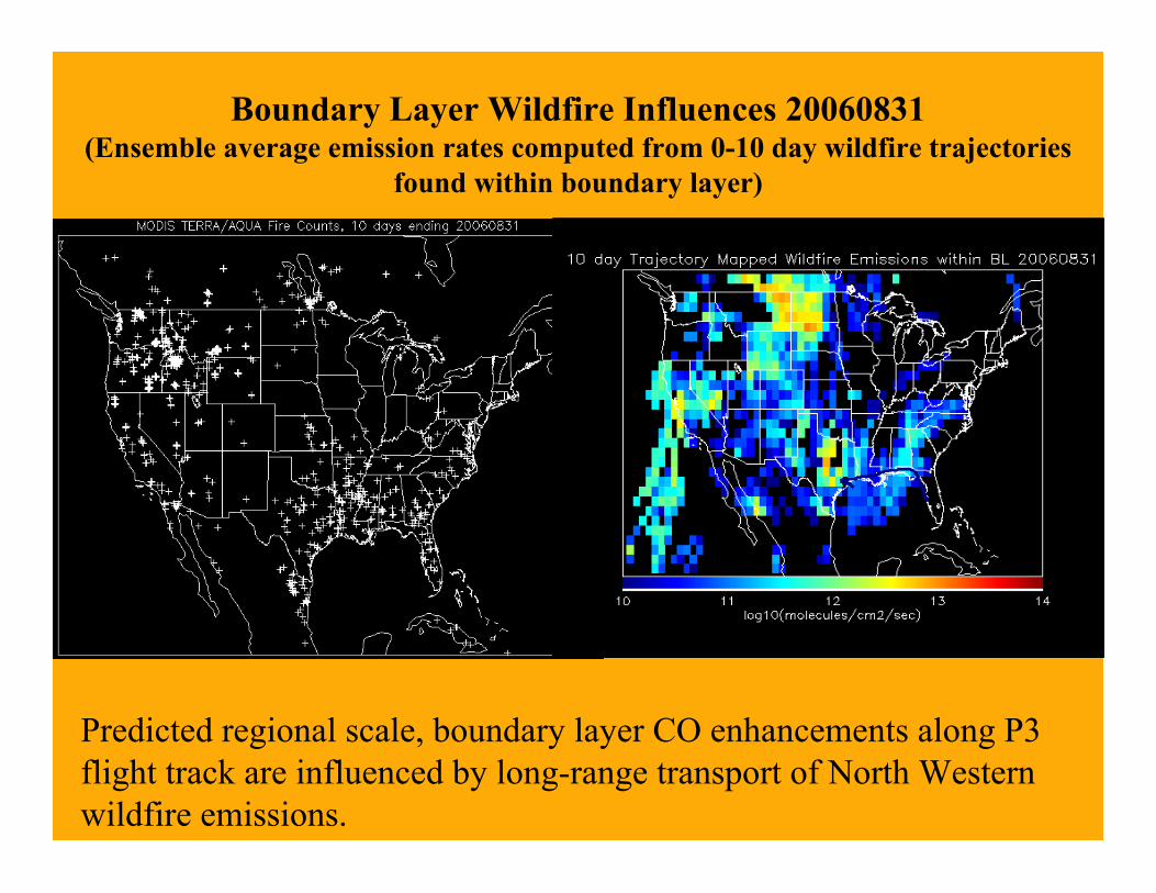
Boundary Layer Wildfire Influences 20060831(Ensemble average emission rates computed from 0-10 day wildfire trajectories
found within boundary layer)
Predicted regional scale, boundary layer CO enhancements along P3flight track are influenced by long-range transport of North Westernwildfire emissions.
Near field Boundary Layer Wildfire Influences 20060831(Ensemble average emission rates computed from 0-48 hr wildfire trajectories
found within boundary layer)
Observed, finescale boundary layer CO enhancements along P3 flighttrack are influenced by recent local biomass burning in NorthernLouisiana.
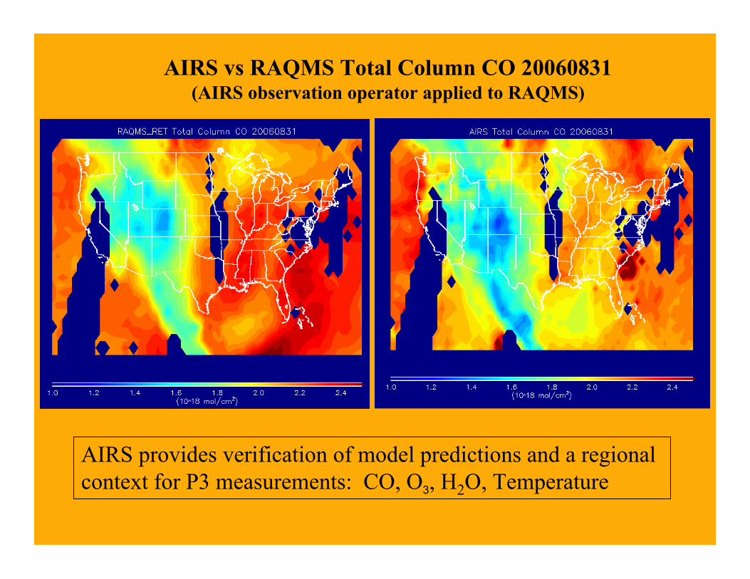
AIRS vs RAQMS Total Column CO 20060831(AIRS observation operator applied to RAQMS)
AIRS provides verification of model predictions and a regionalcontext for P3 measurements: CO, O3, H2O, Temperature
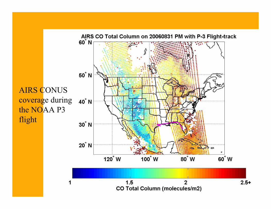
AIRS CONUScoverage duringthe NOAA P3flight
Highaltitude plume
mid-tropdeficit
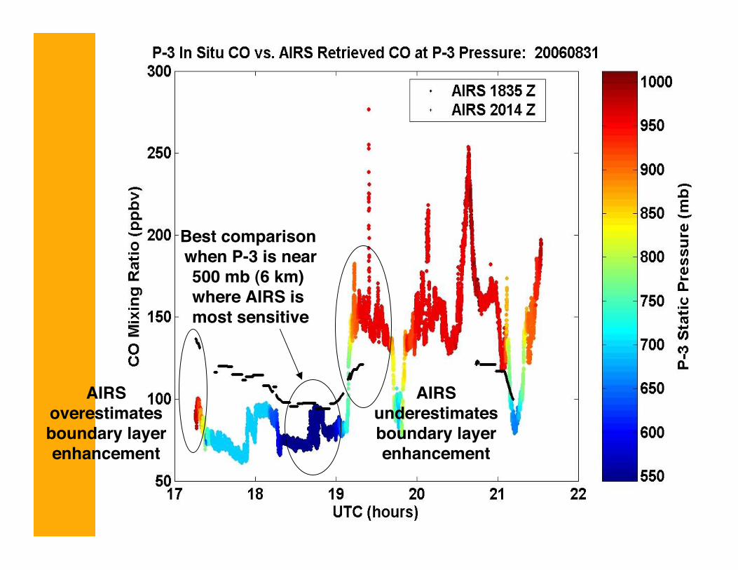
AIRS at 1835 UTC 2014
Boundarylayer
enhancement
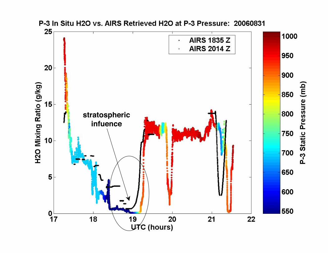
Best comparison when P-3 is near500 mb (6 km) where AIRS is most sensitive
AIRSoverestimatesboundary layerenhancement
AIRSunderestimatesboundary layerenhancement
Summary• Synthesis of Houston AIRNOW, NOAA P3, NASA AIRS
measurements, and RAQMS predictions:– AIRS provides regional context for interpretation of ground and
airborne measurements.– Model and trajectory analysis provides link between local air
quality and regional observations.– Comparisons to P3 guide interpretation of model predictions and
AIRS retrieved boundary layer CO enhancements.
• Results suggest:– Up to 30 ppbv regional scale O3 enhancement contributed to
Houston air quality August 30-September 2, 2006.– Near-field (Louisiana) and remote (Pacific Northwest) biomass
burning contributed to the regional scale enhancement.
Extra slides
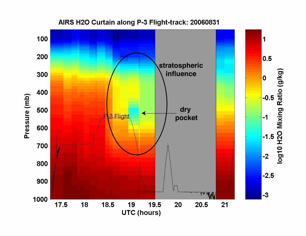
stratosphericinfluence
dry pocket
stratosphericinfuence
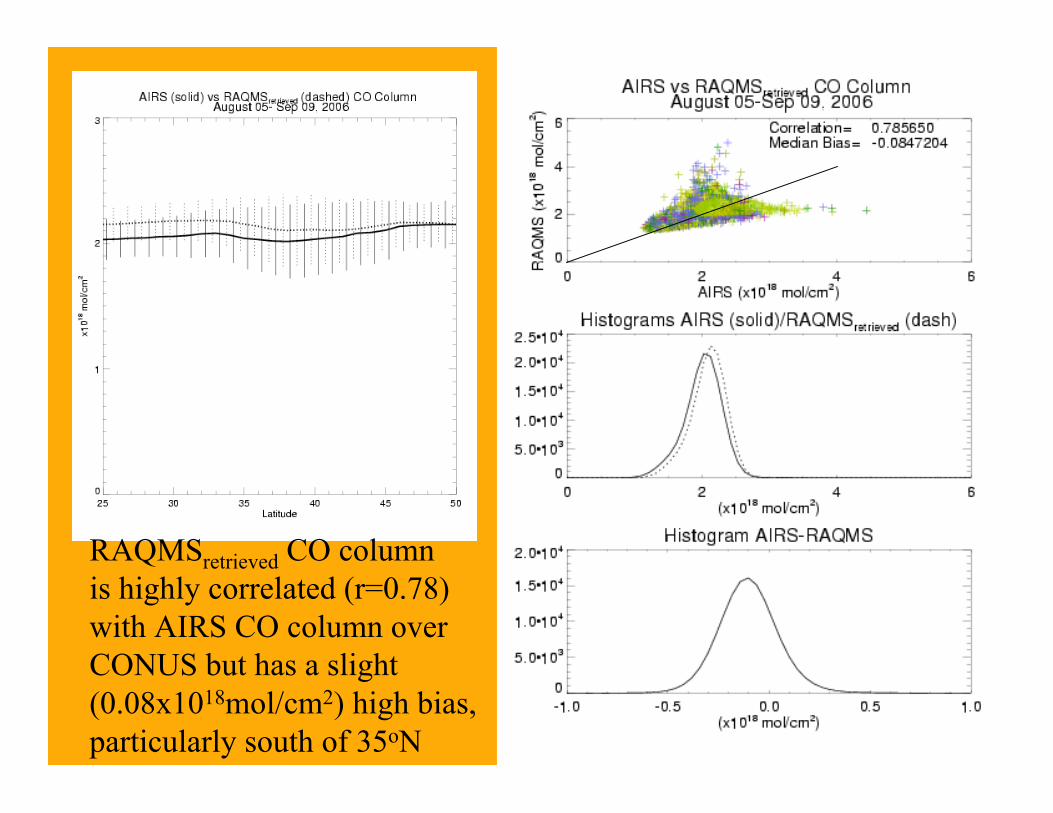
RAQMSretrieved CO column is highly correlated (r=0.78) with AIRS CO column over CONUS but has a slight (0.08x10¹⁸mol/cm2) high bias, particularly south of 35oN
Questions A, C, D, E – Emissions• Modeled isoprene concentrations vs. 2000 observations
(Elena McDonald-Buller)
Comparisons Of Modeled andComparisons Of Modeled andObserved Isoprene ConcentrationsObserved Isoprene Concentrations
In Southeast TexasIn Southeast Texas
The University of Texas at AustinThe University of Texas at AustinCenter for Energy and Environmental ResourcesCenter for Energy and Environmental Resources
andandENVIRON International CorporationENVIRON International Corporation
ObjectiveObjective Compare isoprene concentrations recorded usingCompare isoprene concentrations recorded using
ground and aircraft measurements collected during theground and aircraft measurements collected during theTexas Air Quality Study 2000 to model predictions; thisTexas Air Quality Study 2000 to model predictions; thisprovides the starting point for the science synthesisprovides the starting point for the science synthesisquestions dealing with biogenic emission inventoriesquestions dealing with biogenic emission inventories
Comparisons of predictions of Comparisons of predictions of eulerianeulerian models ( models (CAMxCAMx))with ground and aloft (Electra and G-1) measurementswith ground and aloft (Electra and G-1) measurements
GloBEISGloBEIS v. 3.1 v. 3.1 Land cover/land use data from Land cover/land use data from WiedinmyerWiedinmyer et al. (2001) for Texas et al. (2001) for Texas Surface temperature from interpolation of NWS and other dataSurface temperature from interpolation of NWS and other data PAR fluxes from University of Maryland and NOAA for the GEWEXPAR fluxes from University of Maryland and NOAA for the GEWEX
GCIPGCIP Wind speed and humidity from MM5.Wind speed and humidity from MM5.
Air Quality Modeling:Air Quality Modeling: CAMxCAMx v. 4.03 v. 4.03 August 22-September 6, 2000 episode with nested regional/urbanAugust 22-September 6, 2000 episode with nested regional/urban
gridgrid Base 5b emission inventories from TCEQ SIP modelingBase 5b emission inventories from TCEQ SIP modeling CB-IV chemical mechanismCB-IV chemical mechanism
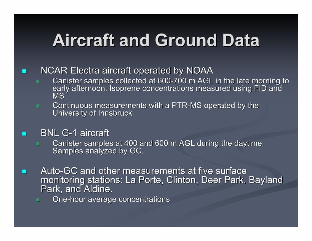
Aircraft and Ground DataAircraft and Ground Data NCAR Electra aircraft operated by NOAANCAR Electra aircraft operated by NOAA
Canister samples collected at 600-700 m AGL in the late morning toCanister samples collected at 600-700 m AGL in the late morning toearly afternoon. Isoprene concentrations measured using FID andearly afternoon. Isoprene concentrations measured using FID andMSMS
Continuous measurements with a PTR-MS operated by theContinuous measurements with a PTR-MS operated by theUniversity of InnsbruckUniversity of Innsbruck
BNL G-1 aircraftBNL G-1 aircraft Canister samples at 400 and 600 m AGL during the daytime.Canister samples at 400 and 600 m AGL during the daytime.
Samples analyzed by GC.Samples analyzed by GC.
Auto-GC and other measurements at five surfaceAuto-GC and other measurements at five surfacemonitoring stations: La Porte, Clinton, Deer Park, monitoring stations: La Porte, Clinton, Deer Park, BaylandBaylandPark, and Aldine.Park, and Aldine.
One-hour average concentrationsOne-hour average concentrations
Modeled Isoprene vs. Surface DataModeled Isoprene vs. Surface DataISOP concentration at Clinton 4km grid cell
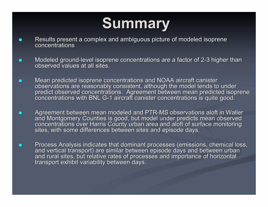
SummarySummary Results present a complex and ambiguous picture of modeled isopreneResults present a complex and ambiguous picture of modeled isoprene
concentrationsconcentrations
Modeled ground-level isoprene concentrations are a factor of 2-3 higher thanModeled ground-level isoprene concentrations are a factor of 2-3 higher thanobserved values at all sites.observed values at all sites.
Mean predicted isoprene concentrations and NOAA aircraft canisterMean predicted isoprene concentrations and NOAA aircraft canisterobservations are reasonably consistent, although the model tends to underobservations are reasonably consistent, although the model tends to underpredict observed concentrations. Agreement between mean predicted isoprenepredict observed concentrations. Agreement between mean predicted isopreneconcentrations with BNL G-1 aircraft canister concentrations is quite good.concentrations with BNL G-1 aircraft canister concentrations is quite good.
Agreement between mean modeled and PTR-MS observations aloft in WallerAgreement between mean modeled and PTR-MS observations aloft in Wallerand Montgomery Counties is good, but model under predicts mean observedand Montgomery Counties is good, but model under predicts mean observedconcentrations over Harris County urban area and aloft of surface monitoringconcentrations over Harris County urban area and aloft of surface monitoringsites, with some differences between sites and episode days.sites, with some differences between sites and episode days.
Process Analysis indicates that dominant processes (emissions, chemical loss,Process Analysis indicates that dominant processes (emissions, chemical loss,and vertical transport) are similar between episode days and between urbanand vertical transport) are similar between episode days and between urbanand rural sites, but relative rates of processes and importance of horizontaland rural sites, but relative rates of processes and importance of horizontaltransport exhibit variability between days.transport exhibit variability between days.
Model sensitivity studiesModel sensitivity studies Model systematically predicts larger groundModel systematically predicts larger ground
concentrations compared to observationsconcentrations compared to observations Modeled mean concentrations are in good agreementModeled mean concentrations are in good agreement
with aircraft measurementswith aircraft measurements Sensitivity studies performed examining bothSensitivity studies performed examining both
uncertainties in the inventory and other modeluncertainties in the inventory and other modeluncertainties:uncertainties: Change vertical mixingChange vertical mixing Systematic Systematic sitingsiting bias for ground stations bias for ground stations Effect of Effect of underpredictionunderprediction of free radical concentrations of free radical concentrations Possible land cover changes and drought effectsPossible land cover changes and drought effects All are potentially important; All are potentially important; TexAQSTexAQS 2000 data do not allow us 2000 data do not allow us
to distinguish between these causesto distinguish between these causes
Implications for Implications for TexAQSTexAQS II II
Need for better characterization of verticalNeed for better characterization of verticalmixing and spatial gradients of isoprene,mixing and spatial gradients of isoprene,as well as chemical loss processes.as well as chemical loss processes. Radical related measurements at MoodyRadical related measurements at Moody
Tower and from NOAA P-3Tower and from NOAA P-3 Vertical mixing structure from LIDAR Vertical mixing structure from LIDAR
measurementsmeasurements Updating of Updating of landcoverslandcovers Measurements of isoprene reaction productsMeasurements of isoprene reaction products
Question B – Mixed Layer Height: Moody Tower data(Ryan Perna, James Flynn)
Question I – Chemical mechanisms: Moody Tower data• Ozone and radical production
(Xinrong Ren, Jingqiu Mao, Bernhard Rappenglueck, Barry Lefer)
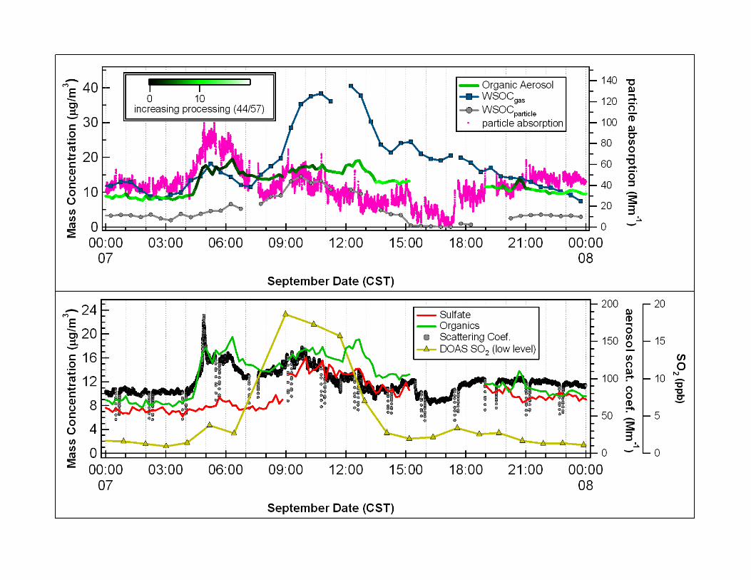
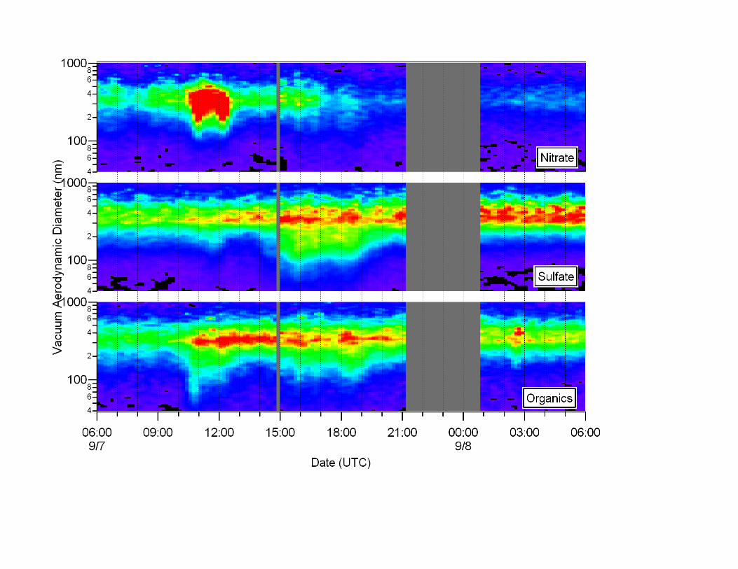
Questions A, C, D, E – Emissions: Moody Tower data• Aerosol production
(Casey Anderson, Luke Ziemba, Dean Atkinson, Olga Pikelnaya)
Some Results from theUH Moody Tower
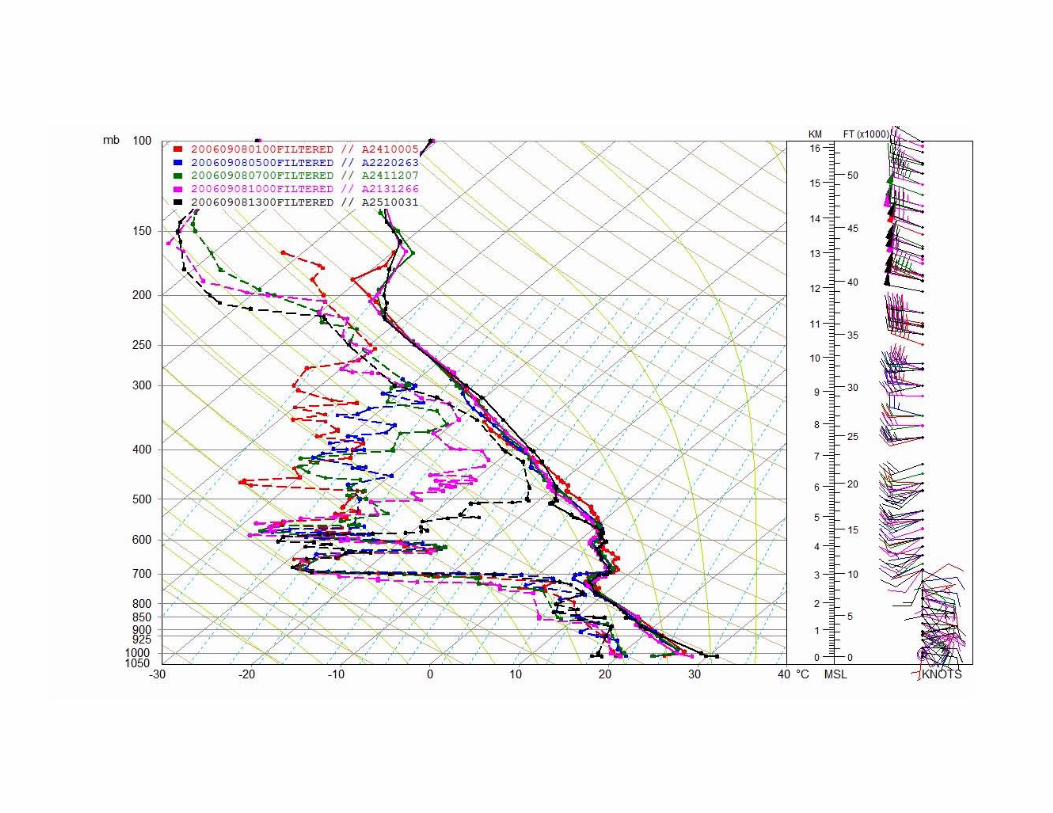
• Meteorology Overview ofSeptember 6-7Ryan Perna, James Flynn
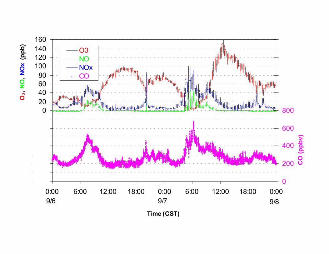
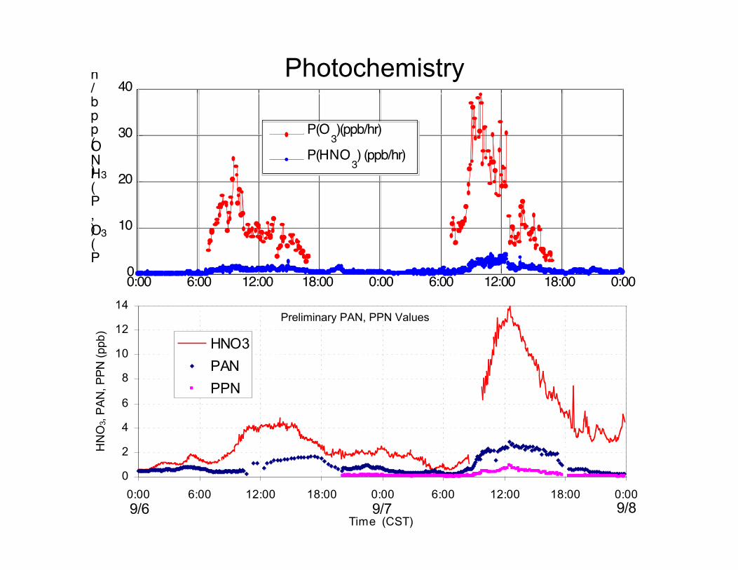
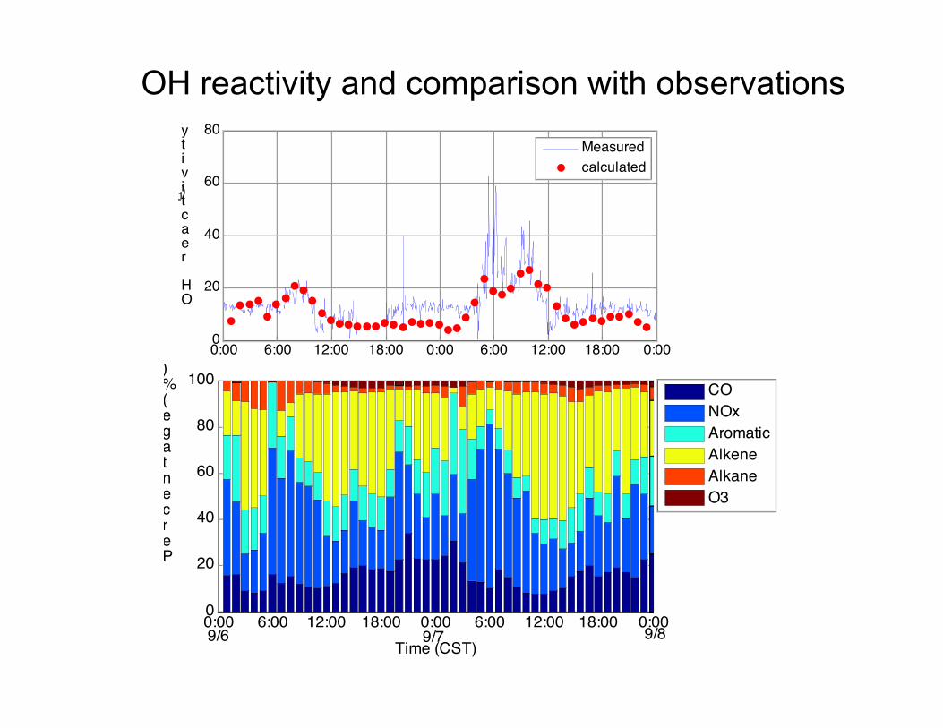
• Photochemical Processes Xinrong Ren, Jingqiu Mao, Bernhard
Rappenglueck, Barry Lefer, JochenStutz, Michael Leuchner
• Aerosol FormationCasey Anderson, Luke Ziemba, DeanAtkinson, Olga Pikelnaya
NOTE: All data preliminary
Preliminary Observed Data at Moody Tower (Sep. 6 – Sep. 7)