COMPUTATIONAL MODELING OF HIP JOINT MECHANICS by Andrew Edward Anderson A dissertation submitted to the faculty of The University of Utah in partial fulfillment of the requirements for the degree of Doctor of Philosophy Department of Bioengineering The University of Utah April 2007
Transcript
COMPUTATIONAL MODELING OF HIP JOINT MECHANICS
by
Andrew Edward Anderson
A dissertation submitted to the faculty of The University of Utah
in partial fulfillment of the requirements for the degree of
The hip joint is one of the largest weight bearing structures in the human body.
While its efficient structure may lend to a lifetime of mobility, abnormal, repetitive
loading of the hip is thought to result in osteoarthritis (OA). The etiology of hip OA is
unknown however, due to the high loads this joint supports, mechanics have been
implicated as the primary factor. Quantifying the relevant mechanical parameters in the
joint (i.e. cartilage and bone stresses) appears to be central to an enhanced understanding
of this disease. Experimental studies have provided valuable insight into baseline hip
joint biomechanics but they require a protocol that is inherently invasive. Numerical
modeling techniques, such as the finite element method, open the possibility of predicting
hip joint biomechanics noninvasively and could revolutionize the way pathological hips
are diagnosed and treated. Unfortunately, hip finite element models to date have used
simplified geometry and have not been validated. It can be credibly argued that prior
computational models of the hip joint do not have the ability to predict cartilage and bone
mechanics with sufficient accuracy for clinical application.
The aim of this dissertation is to develop and validate methods that will facilitate
patient-specific modeling of hip joint biomechanics. Toward this objective, subject-
specific FE models of the pelvis and entire hip joint were developed. The accuracy of
model geometry, i.e. cortical bone and cartilage thickness, was assessed using phantom
based imaging studies. FE predictions were compared directly with experimental data for
purposes of validation. The sensitivity of the models to errors in assumed and measured
model inputs was quantified. Finally, recognizing that acetabular dysplasia may be the
single most important contributor of hip joint OA, the validated modeling protocols were
extended to analyze patient-specific models to demonstrate the general feasibility of the
approach and to quantify differences in hip joint biomechanics between a normal and
dysplastic hip joint. The developed modeling methodologies have a number of potential
longer-term uses and benefits, including improved diagnosis of pathology, patient-
specific approaches to treatment, and prediction of the success rate of corrective surgeries
based on pre- and post-operative mechanics.
v
To my father: Richard E. Anderson
“It matters not how long we live but how” Philip James Bailey
TABLE OF CONTENTS
ABSTRACT....................................................................................................................... iv LIST OF TABLES............................................................................................................. ix LIST OF FIGURES .............................................................................................................x ACKNOWLEDGEMENTS............................................................................................. xiii CHAPTER 1. INTRODUCTION ...................................................................................................1 Motivation................................................................................................................1 Research Goals.........................................................................................................4 Summary of Chapters ..............................................................................................5 References................................................................................................................8 2. BACKGROUND ...................................................................................................10 Forward ..................................................................................................................10 Hip Joint Structure and Function ...........................................................................11 Pelvic and Femoral Bone ...........................................................................11 Cartilage.....................................................................................................13 Labrum, Capsule, Ligaments, Muscles......................................................15 Hip Joint Pathology................................................................................................20 Osteoarthritis..............................................................................................20 Hip Dysplasia.............................................................................................22 Experimental Hip Joint Biomechanics...................................................................25 Bone Material Properties ...........................................................................25 Cartilage Material Properties .....................................................................27 In-Vitro Studies of Hip Joints ....................................................................29 In-Vivo Studies of Hip Joints ....................................................................32 Numerical Modeling of Hip Joint Biomechanics ..................................................35 Analytical Modeling of the Hip Joint ........................................................35 Computational Modeling of the Hip Joint .................................................36 References..............................................................................................................43
3. A SUBJECT-SPECIFIC FINITE ELEMENT MODEL OF THE PELVIS: DEVELOPMENT, VALIDATION AND SENSITIVITY STUDIES......................................................................................58 Abstract ..................................................................................................................58 Introduction............................................................................................................60 Materials and Methods...........................................................................................63 Experimental Study....................................................................................63 Geometry Extraction and Mesh Generation ..............................................66 Position-Dependent Cortical Thickness.....................................................69 Assessment of Cortical Bone Thickness....................................................71 Material Properties and Boundary Conditions...........................................72 Sensitivity Studies......................................................................................73 Data Analysis .............................................................................................75 Results ....................................................................................................................76 Reconstructions of Pelvic Geometry .........................................................76 Cortical Bone Thickness ............................................................................77 Trabecular Bone Elastic Modulus..............................................................80 FE Model Predictions ................................................................................80 Discussion..............................................................................................................85 References..............................................................................................................92 4. FACTORS INFLUENCING CARTILAGE THICKNESS MEASUREMENTS WITH MULTI-DETECTOR CT A PHANTOM STUDY..........................................................................................97 Abstract ..................................................................................................................97 Introduction............................................................................................................99 Materials and Methods.........................................................................................102 Phantom Description................................................................................102 CT Imaging Protocol................................................................................105 Image Segmentation, Surface Reconstruction, and Measurement of Thickness ......................................................................106 Error Analysis ..........................................................................................109 Results ..................................................................................................................110 Contrast Enhanced Scans.........................................................................110 Non-Enhanced Scans ...............................................................................115 Discussion............................................................................................................117 Study Limitations.....................................................................................119 Practical Applications ..............................................................................120 References............................................................................................................122
5. VALIDATION OF FINITE ELEMENT PREDICTIONS OF CARTILAGE CONTACT PRESSURE IN THE HUMAN HIP JOINT...........................................................................................126 Abstract ................................................................................................................126 Introduction..........................................................................................................128 Methods................................................................................................................130 Experimental Protocol .............................................................................130 Computational Protocol ...........................................................................133 Sensitivity Studies....................................................................................136 Data Analysis ...........................................................................................137 Results ..................................................................................................................140 FE Mesh Characteristics ..........................................................................140 Peak Pressure, Average Pressure, Contact Area......................................141 Contact Patterns .......................................................................................142 Misalignment and Magnitude Errors .......................................................145 Sensitivity Studies- Cartilage Material Properties and Thickness...........147 Sensitivity Studies- FE Boundary Conditions .........................................149 Discussion............................................................................................................152 References............................................................................................................159 6. PATIENT-SPECIFIC FINITE ELEMENT MODELING PROOF OF CONCEPT .......................................................................................165 Abstract ................................................................................................................165 Introduction..........................................................................................................167 Methods................................................................................................................170 Subject-Selection .....................................................................................170 CT Arthrography......................................................................................170 Image Data Analysis and Segmentation ..................................................171 FE Mesh Generation, Cartilage Thickness, Material Properties..............172 FE Boundary and Loading Conditions ....................................................174 Sensitivity Studies....................................................................................175 Data Analysis ...........................................................................................175 Results ..................................................................................................................177 Discussion............................................................................................................182 References............................................................................................................189 7. DISCUSSION......................................................................................................195 Summary ..............................................................................................................195 Limitations and Future Work...............................................................................200 References............................................................................................................205
LIST OF TABLES Table Page 3.1. Models studied for sensitivity analysis ...............................................................75
3.2. Reconstruction errors for simulated cortical bone ..............................................78
3.3. Results for all sensitivity models ........................................................................84
5.1. Misalignment and magnitude errors of FE predicted cartilage contact pressures ................................................................................146 5.2. Differences of center of pressures between FE and experimental results ...................................................................................146 6.1. Differences in FE predicted mechanics between a normal and dysplastic hip joint .........................................................................179
viii
LIST OF FIGURES Figure Page 2.1. Photograph of plastic hip joint............................................................................12
2.2. Histological cross-section of cartilage ................................................................14
2.3. Illustration of hip joint with labrum....................................................................16
2.4. Illustration of hip joint capsule ...........................................................................17 2.5. Illustration of iliofemoral ligament.....................................................................18 2.6. Volumetric CT scan of patient with acetabular retroversion ..............................24 3.1. Schematic of pelvis loading fixture ....................................................................65
3.2. 3D reconstruction of pelvis from CT image data................................................67
3.3. Finite element mesh of pelvis with close-up of acetabulum...............................68 3.4. Schematic illustrating the special cases considered in in determination of cortical thickness .................................................................70 3.5. Cortical bone thickness phantom........................................................................71 3.6. Schematic showing length measurements obtained from cadaveric pelvis and accuracy of geometry reconstruction.................................................76 3.7. Contours of position dependent cortical bone thickness of the pelvis.........................................................................................................79 3.8. Distribution of pelvic Von-Mises stress .............................................................82 3.9. Finite element predicted vs. experimentally measured strains for subject-specific and sensitivity models .........................................................83
4.1. Schematic of phantom used to assess accuracy of cartilage thickness reconstructions ...............................................................104 4.2. Simulated cartilage RMS and mean residual reconstruction errors for the transverse contrast enhanced CT scans as a function of agent concentration......................................................................111 4.3. Simulated cartilage RMS and mean residual reconstruction errors for the transverse contrast enhanced CT scans as a function of imaging direction and resolution .................................................112 4.4. Simulated cartilage RMS and mean residual reconstruction errors for the transverse contrast enhanced CT scans as a function of joint spacing, agent concentration, imaging direction and resolution ......................................................................114 4.5. Simulated cartilage RMS and mean residual reconstruction errors for the transverse non-contrast enhanced CT scans as a function of imaging direction and resolution .................................................116 5.1. Experimental setup for loading of hip joint ......................................................132 5.2. Finite element mesh of the entire hip joint in the walking position with a close-up of the acetabulum.......................................................135 5.3. Contours of cartilage thickness.........................................................................140 5.4. Finite element vs. experimentally measured average pressure and contact area ..................................................................................141 5.5. Qualitative comparison between finite element and experimentally measured contact pressure .......................................................143 5.6. Finite element predicted pressures relative to the femur and acetabulum .................................................................................................144 5.7. Percent changes in peak pressure, average pressure and and contact area due to changes in cartilage material properties and geometry......................................................................148 5.8. Percent changes in peak pressure, average pressure and and contact area due to changes in model boundary conditions..........................................................................................150
xi
5.9. Contours of cartilage pressure predicted by the baseline and rigid bone finite element models................................................................151 6.1. Fringe plots of acetabular and femoral cartilage thickness for the normal and dysplastic hip joints............................................................173 6.2. Comparison of finite element predicted acetabular cartilage pressures between a normal and dysplastic hip joint ........................................177 6.3. Finite element predicted acetabular cartilage pressures as a function of anatomical and joint reaction force orientation for the normal and dysplastic hip joint ...........................................180
xii
ACKNOWLEDGEMENTS
Financial support from the University of Utah Department of Orthopaedics,
University of Utah Funding Incentive Seed Grant, the Orthopaedic Research and
Education Foundation, and from NIH Grant #F31-EB00555 is gratefully acknowledged.
The University of Utah Department of Radiology (CAMT), Scientific Computing
Imaging Institute (SCI) and Brad Maker of Lawrence Livermore National Lab are also
given acknowledgement for their contributions.
CHAPTER 1
INTRODUCTION
MOTIVATION
The hip joint serves a very important biomechanical function. While supporting
the majority of the human body (~ 2/3 of total bodyweight) the joint must simultaneously
facilitate smooth articulation of the lower limbs to enable bi-pedal gait. During routine
daily activities, forces on the order of 5.5 times bodyweight are transferred between the
femur and pelvis [1-3]. While its efficient structure may lend to a lifetime of mobility,
abnormal, repetitive loading of the hip is thought to result in the breakdown of articular
cartilage, resulting in osteoarthritis (OA) [4-7].
Hip joint OA represents a significant burden to society via financial, social and
psychological effects. It is estimated that nearly 40 million Americans currently have
joint osteoarthritis (~18% of the population) of which nearly 3% of the cases originate at
the hip joint [8,9]. To alleviate pain and return the hip to at least the most basic
functioning state, nearly 193,000 osteoarthritic hips are replaced annually in the United
States by way of total hip arthroplasty (THA) [10]. While THA has enjoyed a high rate
of success in elderly patients (less than 10% require revision THA [10]), the surgery is
generally avoided in the younger population due to the limited lifespan of implants and
2
unfavorable results of revision THA. Although a common misconception by the general
public, hip OA is not confined to elderly patients. As detailed later, factors such as
abnormal joint geometry (i.e. hip dysplasia), body weight, occupation, and prior injury
appear to play major roles independently of age [11-13]. Nevertheless, the etiology of
hip OA is unknown, in part because it takes so long to develop- a decade or more likely
passes before cartilage has fissured to the point where bone contact initiates pain [14].
However, due to the high loads this joint supports, mechanical factors have been
implicated as a primary causes [4-7]. Thus, quantifying the relevant mechanical
parameters in the joint (i.e. cartilage and bone stresses) appears to be central to an
enhanced understanding of this disease [14].
Research on the biomechanics of the hip is not new to orthopedic medicine.
While previous studies have provided valuable insight into baseline hip joint
biomechanics, they require a protocol that is inherently invasive. Unlike experimental
investigations, computational modeling opens the possibility of predicting hip joint
biomechanics noninvasively. In particular, the advent, increased availability and
resolution medical imaging modealities provide a means to develop detailed
computational models that are based on individual patient geometry. These attractive
points, along with a tremendous evolution of computing power, have lead to substantial
growth in the field of computational biomechanics.
Although computational models have provided substantial additional insight to
hip biomechanics above and beyond that obtained via experimental studies, substantial
voids remain. In particular, simplifying model assumptions have often resulted in model
3
predictions that are inconsistent with experimental measurements. Most models have not
been validated by direct comparison with experimental data. For an analyst to develop
patient-specific models, without having to validate each model independently, it is
necessary to demonstrate that: 1) the computational protocol yields results that predict
known/measured quantities with sufficient accuracy, and 2) an assessment of model error
and uncertainty is accounted for in an effort to gauge how inaccuracies could be
propagated due to erroneous model inputs and assumptions.
4
RESEARCH GOALS
The overall aim of this dissertation is to develop and validate methods that will
facilitate patient-specific modeling of hip joint biomechanics. It is clear that patient-
specific computational models have the potential to revolutionize the way that disorders
of the hip joint are diagnosed and treated. However, first rigorous and validated
protocols that incorporate both computational and experimental techniques must be
established. In this dissertation research, model predictions are compared directly with
experimental data and errors in assumed and measured model inputs, i.e. material
properties, constitutive behavior, geometry, and boundary conditions, are discussed as
they pertain to errors in the developed model and in the context of future patient
modeling efforts. Second, recognizing that acetabular dysplasia may be the single most
important contributor of hip joint OA [17-20], the validated subject-specific finite
element modeling protocol is extended to analyze patient-specific models to demonstrate
the general feasibility of the approach and to quantify differences in hip joint
biomechanics between a normal subject and a patient with acetabular dysplasia. Finally,
limitations of the modeling protocol as well as unforeseen challenges in modeling
individual patients non-invasively are presented in the context of general hip joint
modeling applications but with special emphasis to the study of acetabular dysplasia.
5
SUMMARY OF CHAPTERS
The structure of this dissertation has been organized to answer the essential
questions that arise when developing a protocol to generate patient-specific models of the
hip joint. The primary objective of Chapter 2 is to provide a working knowledge base
that will serve as reference to the topics covered in the remaining Chapters. Chapter 2
discusses hip joint structure and function and provides further motivation for developing
computational models, in particular, by application of the finite element method. Topics
such as hip osteoarthritis, approaches to quantify hip biomechanics (experimental and
computational), and the importance of computational model verification, validation, and
sensitivity studies are presented.
In the context of hip joint OA, the most fundamental mechanics of interest are
bone and cartilage stresses and strains. In this dissertation computational models are
developed and validated to study the mechanics of bone and cartilage separately in an
effort to maintain simplicity and to control confounding factors (Chapter 3 and Chapter 5,
respectively). Chapter 3 discusses the development and validation of a subject-specific
finite element model of the pelvis. Computational predictions of bone strains were
validated by direct comparison to experimentally measured strains using tri-axial strain
gauges attached to the cortical surface of the pelvis. The influence of measured and
assumed model inputs was assessed using sensitivity studies and the geometrical
accuracy of the model, in particular, cortical bone thickness, was quantified.
Since computational models often use medical image data as the basis for creating
model geometry, it is crucial to demonstrate that the reconstructed geometry is an
6
accurate representation of the true continuum. Although this is important for all
computational studies, it becomes absolutely essential when modeling joint contact
mechanics between layers of articulating cartilage. Although volumetric computed
tomography (CT) data are often used as the basis for constructing joint models, the lower
bounds for detecting articular cartilage thickness and the influence of imaging parameters
on the ability to image cartilage have yet to be reported. Thus, it was necessary to
quantify the accuracy and detection limits of cartilage geometry with CT. To this end, a
phantom based imaging study was conducted and is presented in Chapter 4. While the
results of this study have application to subject-specific models using cadaveric joints
(Chapter 5), the primary focus of this work was centered around quantifying the accuracy
of CT arthrography since this procedure is required to visualize cartilage in live patients,
which has direct relevance to patient-specific modeling (Chapter 6). The results of this
study are discussed in terms of general clinical applications of CT for imaging articular
cartilage in diarthrodial joints.
Chapter 5 presents results for a subject-specific finite element model of the
mechanics of cartilage in the hip joint. Finite element predictions of cartilage contact
pressures were validated by comparing computational predictions to experimentally
measured contact pressures using pressure sensitive film. A physiological experimental
and computational loading protocol was employed in an effort to lay the groundwork
necessary for creating realistic patient-specific models. Sensitivity studies were included
in the analysis to determine the influence of measured and assumed model inputs on the
7
ability to predict cartilage contact pressures. Chapter 5 concludes with a discussion of
the model’s limitations.
As discussed in Chapter 2, acetabular dysplasia may be the primary etiology of
hip joint OA. Therefore, it was of interest to demonstrate the feasibility of the modeling
protocol developed in Chapters 3-5 for application to individual patients with dysplasia.
Chapter 6 presents two patient-specific finite element models: one for a normal volunteer
and one for a patient with acetabular dysplasia. Differences in computationally predicted
bone and cartilage mechanics are reported and clinical implications of these data are
discussed. Chapter 6 concludes with a discussion of the challenges involved with patient-
specific modeling and makes recommendations for circumventing these issues in the
context of future modeling efforts. Finally, Chapter 7 summarizes the entire dissertation
by highlighting the important contributions that were made to the field of hip
computational biomechanics along with a discussion of limitations and future research
directions.
8
REFERENCES
[1] Hodge, W. A., Fijan, R. S., Carlson, K. L., Burgess, R. G., Harris, W. H., and
Mann, R. W., 1986, "Contact Pressures in the Human Hip Joint Measured in Vivo," Proc Natl Acad Sci U S A, 83, pp. 2879-83.
[2] Bergmann, G., Deuretzbacher, G., Heller, M., Graichen, F., Rohlmann, A.,
Strauss, J., and Duda, G. N., 2001, "Hip Contact Forces and Gait Patterns from Routine Activities," J Biomech, 34, pp. 859-71.
[3] Bergmann, G., 1998, Hip98: Data Collection of Hip Joint Loading on CD-Rom.
Free University and Humboldt University, Berlin. [4] Mankin, H. J., 1974, "The Reaction of Articular Cartilage to Injury and
Osteoarthritis (Second of Two Parts)," N Engl J Med, 291, pp. 1335-40. [5] Mankin, H. J., 1974, "The Reaction of Articular Cartilage to Injury and
Osteoarthritis (First of Two Parts)," N Engl J Med, 291, pp. 1285-92. [6] Mow, V. C., Setton, L. A., Guilak, F., and Ratcliffe, A., 1995, "Mechanical
Factors in Articular Cartilage and Their Role in Osteoarthritis," in Osteoarthritic Disorders. American Academy of Orthopaedic Surgeons.
[7] Poole, A. R., 1995, "Imbalances of Anabolism and Catabolism of Cartilage
Matrix Components in Osteoarthritis," in Osteoarthritic Disorders. American Academy of Orthopaedic Surgeons.
[8] Felson, D. T., Lawrence, R. C., and Dieppe, P. A., 2000, "Osteoarthritis: New
Insights. Part 2. Treatment Approaches," Ann Internal Med, 133, pp. 726-737. [9] Felson, D. T., Lawrence, R. C., and Dieppe, P. A., 2000, "Osteoarthritis: New
Insights. Part I the Disease and Its Risk Factors," Ann Internal Med, 133, pp. 635-646.
[10] AAOS, 2007,"Questions and Answers about Hip Replacement," National Institute
of Arthritis and Musculoskeletal and Skin Disorders. [11] Anderson, J. J. and Felson, D. T., 1988, "Factors Associated with Osteoarthritis of
the Knee in the First National Health and Nutrition Examination Survey (Hanes I). Evidence for an Association with Overweight, Race, and Physical Demands of Work," Am J Epidemiol, 128, pp. 179-89.
9
[12] Felson, D. T., 1994, "Do Occupation-Related Physical Factors Contribute to Arthritis?," Baillieres Clin Rheumatol, 8, pp. 63-77.
[13] Heliovaara, M., Makela, M., Impivaara, O., Knekt, P., Aromaa, A., and Sievers, K., 1993, "Association of Overweight, Trauma and Workload with Coxarthrosis. A Health Survey of 7,217 Persons," Acta Orthop Scand, 64, pp. 513-8.
[14] Macirowski, T., Tepic, S., and Mann, R. W., 1994, "Cartilage Stresses in the
Human Hip Joint," J Biomech Eng, 116, pp. 10-8. [15] Oberkampf, W. L., Trucano, T. G., and Hirsch, C., "Verification, Validation, and
Predictive Capability in Computational Engineering and Physics," presented at Foundations for Verification and Validation in the 21st Century Workshop, Johns Hopkins University, Laurel, Maryland, 2002.
[16] Anderson, A., Ellis, B. J., and Weiss, J. A., 2006, "Verification, Validation and
Sensitivity Studies in Computational Biomechanics," Computer Methods in Biomechanics and Biomedical Engineering, In Press Dec 2006.
[17] Harris, W. H., 1986, "Etiology of Osteoarthritis of the Hip," Clin Orthop, pp. 20-
33. [18] Murray, R. O., 1965, "The Aetiology of Primary Osteoarthritis of the Hip," Br J
Radiol, 38, pp. 810-24. [19] Solomon, L., 1976, "Patterns of Osteoarthritis of the Hip," J Bone Joint Surg Br,
58, pp. 176-83. [20] Stulberg, S. D. and Harris, W. H., "Acetabular Dysplasia and Development of
Osteoarthritis of the Hip," presented at Proceedings of the second open scientific meeting of the Hip Society, St Louis, MO, 1974.
CHAPTER 2
BACKGROUND
FORWARD
As discussed below, computational models have the potential to non-invasively
estimate hip mechanics for living subjects. However, based on the available in-vivo and
in-vitro experimental data, it can be credibly argued that most previous hip joint
computational models do not have the ability to predict cartilage and bone mechanics
with sufficient accuracy for clinical application. Furthermore, models that have included
more realistic geometries have not been validated by direct comparison to experimental
data. The purpose of this dissertation is to present novel methods to develop and validate
computational models of the hip joint that result in models that indeed have direct clinical
applicability to study diseases such as osteoarthritis (OA) and hip dysplasia. This chapter
presents the most relevant background information, including: hip joint structure and
function, hip pathologies, experimental hip joint biomechanics, and numerical modeling
of hip joint biomechanics.
11
HIP JOINT STRUCTURE AND FUNCTION
The hip is a ball and socket joint formed by the articulation of the spherical head
of the femur and the concave acetabulum of the pelvis. It forms the primary connection
between the lower limbs and skeleton of the upper body. Both the femur and acetabulum
are covered with a layer of cartilage to provide smooth articulation and to absorb load.
The entire hip joint is surrounded by a fibrous, flexible capsule to permit large ranges of
motion but to prohibit the proximal femur from dislocation. Several ligaments connect
the pelvis to femur to further stabilize the joint and capsule. Muscles and tendons
provide actuation forces for extension/flexion, adduction/abduction and internal/external
rotation.
Pelvic and Femoral Bone
The pelvis forms a girdle which protects the digestive and female reproductive
organs. It is formed from three bones: the ilium, ischium and pubis, which fuse together
to form the ox coxae, or innominate bone (Figure 2.1). At the point of fusing they form
the acetabulum (Figure 2.1). Joints adjacent to the pelvis include the sacroiliac (SI) and
pubis joint (Figure 2.1). Many large nerves and blood vessels pass through the pelvis to
the lower limbs.
The femur is the longest and strongest bone in the human body. It consists of a
head and a neck proximally, a diaphysis (or shaft), and two condyles (medial and lateral)
distally. The diaphysis of femur is a simplistic, cylindrical structure, while the proximal
femur is irregular in shape, consisting of a spherical head, neck and lateral bony
12
protrusions termed the greater and lesser trochanters. The trochanters serve as the site of
major muscle attachment. The lateral location of these structures offers a mechanical
advantage to assist with abducting the hip [2].
The bony structure of the pelvis is similar to a sandwich composite material,
consisting of a dense, stiff, thin shell of cortical bone (0.7 to 3.2 mm thick, [3]) filled with
much less dense trabecular bone. The spherical head of the femur has a thin layer of
subchondral bone where cartilage attaches, which is less stiff than cortical bone. Cortical
bone along the diaphysis of femur is much thicker (up to ~ 7 mm [4]) and supports the
large tensile and compressive loads that develop as a result of hip loading. Trabecular
Ilium
Fem
ur
Pubis Joint
Sacro-Iliac Joint
Pubis
Ischium
Acetabulum
Figure 2.1. Photograph of a plastic hip showing the individual bones and joints.
13
bone is found throughout the pelvis and proximal femur but is not as prevalent along the
diaphysis of the femur as this area primarily contains marrow.
Cartilage
Cartilage is composed of collagenous fibers and chondrocytes embedded in a firm
gel (Figure 2.2). Cartilage has remarkable mechanical properties in that it is strong but
flexible and has extremely low coefficients of friction [5]. Cartilage is avascular and
anueral [6]. Chondrocytes and their precursor chondroblasts are the only cells in
cartilage (Figure 2.2) [5]. Nutrients diffuse through the matrix by way of interstitial
fluid, which makes up nearly 60-80% of the total weight of cartilage [7]. In addition,
ionic charges in the fluid are thought to facilitate nutrient flow [8]. The solid matrix
represents nearly 60% of the dry weight and is composed of proteoglycans, which are
large proteins with a protein backbone and glycosaminoglycan (GAG) side chain [7].
The most common GAGs are keratin sulfate and chondroitin sulfate [7]. Matrix fibers
make up the remaining dry weight and are composed of collagen type II [7].
The acetabulum is covered with a horseshoe shaped layer of articulating hyaline
cartilage ranging from 1.2 to 2.3 mm thick in normal adults [9]. The entire head of the
femur is covered with a smooth layer of hyaline cartilage of varying thickness, except for
a small depression called the fovea capitis femoris that gives attachment to the
ligamentum teres. The thickness of femoral cartilage ranges from 1.0 to 2.5 in the normal
adult [9].
14
Figure 2.2. Through the thickness histological photograph of bovine articularcartilage (stained with Alician Blue). Chondrocytes appear as small dots.Copyright Lutz Slomianka 1998-2006.
Cal
cifie
d C
artil
age
Subc
hond
ral B
one
Cartilage Matrix
15
Labrum, Capsule, Ligaments, Muscles
The hip joint labrum is a ring of fibrocartilagenous tissue that surrounds the rim of
the acetabulum (Figure 2.3). It helps to guide normal motion, to prevent dislocation
between the femoral head and acetabulum and is thought to act as a seal to prevent loss of
interstitial fluid. An in vitro study where the labrum was removed have demonstrated
that cartilage is strained to a greater degree than joints with intact labrums for a given
load [10], suggesting that greater fluid flow in the latter scenario causes increased
cartilage matrix deformation.
The entire hip joint is surrounded by the hip capsule (Figure 2.4). The capsule
attaches proximally to entire periphery of the acetabulum, beyond the acetabular labrum.
It also covers the femoral head and neck like a sleeve, eventually attaching to the base of
the femoral neck. The capsule consists of two sets of fibers: longitudinal and circular
fibers. Circular fibers form a collar around the femoral neck whereas longitudinal
retinacular fibers travel along the neck and carry blood vessels.
The capsule is further defined by ligaments. The iliofemoral ligament attaches
from the pelvis to the femur and resists excessive extension (Figure 2.5). It is the
strongest ligament in the human body and allows one to maintain posture for extended
periods without extensive muscular fatigue. The pubofemoral ligament is the most
anterior and inferior portion of the fibrous capsule. It attaches to the pubic bone and
passes inferolaterally to merge with the iliofemoral portion of the fibrous capsule
(attaching to intertrochanteric line). Overabduction of the hip joint is prevented by this
ligament. The ischiofemoral ligament attaches from the ischial part of the acetabulum to
16
the femur and supports the posterior aspect of hip capsule. Finally, the ligament teres
connects the head of the femur to the acetabulum (Figure 2.3). Although it supports little
or no loads it may serve as an important conduit to supply blood to the head of the femur
in some individuals.
Labrum
Figure 2.3. Illustration of hip joint with labrum. Adopted from [1].
17
Figure 2.4. Illustration of hip joint capsule. Adopted from [1].
18
Figure 2.5. Illustration of iliofemoral ligament. Adopted from [1].
19
The hip can flex, extend, abduct, adduct, and rotate using several muscles
attached between the pelvis and femur. Many of the hip muscles are responsible for more
than one type of movement in the hip as different areas of the muscle act on tendons in
different ways. Hip joint flexors include the psoas major, iliacus, rectus femoris,
sartorius, pectineus, adductores longus and brevis, and the anterior fibers of the glutaei
medius and minimus. Hip joint extensors include the glutaeus maximus, assisted by the
hamstring muscles and the ischial head of the adductor magnus. The adductors include
the adductores magnus, longus, and brevis, the pectineus, the gracilis, lower part of the
glutaeus maximus, the glutaei medius and minimus, and the upper part of the glutaeus
maximus. The rotators that cause inward rotation are the glutaeus minimus, anterior
fibers of the glutaeus medius, tensor fasciae latae and the iliacus and psoas major.
Finally, inward rotators include the posterior fibers of the glutaeus medius, the piriformis,
obturatores externus and internus, gemelli superior and inferior, quadratus femoris,
glutaeus maximus, the adductores longus, brevis, and magnus, the pectineus, and the
Sartorius.
20
HIP JOINT PATHOLOGY
The hip is subject to disease due to improper development, acute trauma and
prolonged mechanical wear and tear. The most common disorders include arthritis
dysplasia of the hip and femoro-acetabular impingement. Osteoarthritis and hip dysplasia
are the primary thrust of this dissertation, and thus will be the focus of further discussion.
Osteoarthritis
Osteoarthritis is the most common type of arthritis in the hip and is intimately
associated with other disorders such as avascular necrosis, slipped epiphysis,
impingement and dysplasia. It is also the most common cause of musculoskeletal pain in
the United States [11]. Hip OA is a disorder of the entire joint, involving cartilage, bone,
synovium, labrum, and capsule [12]. OA is classically associated with more advanced
age but is being seen and treated more frequently in younger patients [12].
OA is characterized by a loss of articular cartilage in the predominately load
bearing areas of the joint, with eburnation of the underlying subchondral bone and a
proliferative response characterized by osteophytosis [13,14]. Gradual loss of the matrix
components is thought to be caused by a loss of proteoglycans, although some changes in
the integrity of collagen network may be necessary to initiate the disease [15]. It is also
thought that OA disrupts the mechanism for fluid support, which may exacerbate solid
matrix degeneration [12]. OA is further characterized by an increase in vascularity of
21
surrounding bone. Cysts often form within the surrounding bone and are accompanied by
changes to the joint margin. They may also cause outgrowths of cartilage as well as
osteophyte formation, which may lead to further degeneration. Therefore, the mechanics
of bone in areas adjacent to cartilage may be important to developing a comprehensive
understanding of hip OA.
OA was once thought to be primary or idiopathic in nature. However,
considerable clinical, epidemiological, and experimental evidence supports the concept
that mechanical demand greater than some critical level has a major role in the
development and progression of joint degeneration in all forms of OA. Surveys of
individuals with physically demanding occupations, including farmers, construction
workers, metal workers, miners, and pneumatic drill operators, suggest that repetitive
intense loading is associated with early onset of joint degeneration [16-18]. Excessive
mechanical stress can directly damage articular cartilage and subchondral bone and can
adversely alter chondrocyte function including the balance between synthetic and
degradative activity [19-25].
Although joint loading or overloading can lead to cartilage degeneration, the
precise mechanism remains controversial. Opinions differ concerning the relative
contributions of direct mechanical trauma to articular cartilage versus elevation of
articular stresses secondary to stiffening of subchondral bone. No experimental studies to
date have allowed one to directly separate the contributions of hydrostatic and deviatoric
stresses generated by joint loading. Therefore, it is unknown whether degenerative
22
changes are primarily due to excessive loads applied during normal activities or shearing
of cartilage during abnormal motions involving local instability.
In the elderly patient population, hip OA is treated by prosthetic replacement of
the hip joint. Nearly 193,000 total hip arthroplasties (THA) are performed each year in
the United States [26]. THA is highly successful in relieving pain and restoring
movement. However, ongoing problems with wear and particulate debris may eventually
necessitate further surgery, including replacement of the prosthesis. Men and patients
who weight more than 165 pounds have higher rates of failure [27]. The chance of a hip
replacement lasting 20 years is about 80% [27].
Hip Dysplasia
Developmental dysplasia of the hip (DDH) describes a broad spectrum of
problems, including hips that are unstable, malformed, subluxated (incomplete
dislocation), or completely dislocated [28]. In the broadest sense, DDH is a
developmental deformity characterized by malorientation and a reduction of contact area
between the femur and acetabulum [29]. Subluxation caused by dysplasia of the hip joint
is a primary cause of degenerative joint disease and clinical disability [30]. Subluxation
leads to increased stresses across the hip joint each time the hip is loaded during gait [31].
Consequently, it is thought that the altered biomechanics cause cartilage and bone of the
hip to break down prematurely, leading to early hip osteoarthritis. OA due to hip
dysplasia is commonly treated by THA. Surgical correction of the anatomic
abnormalities associated with hip dysplasia is performed on younger patients via pelvic
23
osteotomy, which preserves the hip joint and associated articular cartilage and delays the
need for prosthetic replacement of the hip. Redirectional acetabular osteotomy
(periacetabular osteotomy) involves cutting the socket free from the pelvis and rotating it
to a new orientation [32-37]. The most common type of dysplasia, referred to herein as
traditional dysplasia, can be diagnosed by evaluation of a 2-D planar radiograph of the
hip. Recently, a specific variant of dysplasia, referred to herein as retroversion of the
acetabulum, has been identified [38,39]. In the retroverted acetabulum, the acetabular
opening and its proximal roof lie at an angle of retroversion with respect to the sagittal
plane. Thus, posterior coverage of the femoral head is lost (Figure 2.6).
Retroversion is difficult to diagnose by the untrained clinician since a standard hip
radiograph shows that the hip is normal; nevertheless, the anatomy of the retroverted
acetabulum is still pathologic. It is likely that the obscurity of the retroverted acetabulum
has often persuaded the clinician into prescribing passive treatments for a potentially
aggressive pathology.
Several studies have shown that mild developmental dysplasia, in patients that
went unrecognized before, may indeed be the leading cause of osteoarthritis in the hip
[39-43]. Wilson and Poss [44] reported that deformity of the acetabulum is found in 25-
35% of adult cases of OA of the hip. Michaeli et al. [29] estimated that 76% of patients
with OA of the hip have some type of untreated acetabular dysplasia. In contrast to these
reports, other studies have failed to find a statistically significant relationship between
acetabular dysplasia and the risk of hip OA [45-49]. These discrepancies highlight the
need for an improved understanding of hip dysplasia.
24
Figure 2.6. Anterior (A) and Posterior (B) view of a volumetric CT scan from a patient with acetabular retroversion of the left hip. The patient’s right hip was considered normal. The lines indicate the edge of the acetabulum. Note excessive forward progression of anterior edge of left acetabulum in image A) and lack of posterior wall coverage of left femur in image B). Courtesy of Christopher L. Peters.
Left Right
LeftRight
AnteriorA)
B)
Posterior
25
EXPERIMENTAL HIP JOINT BIOMECHANICS
The contribution of muscles, ligaments, tendons, and hip capsule serve as vital
components when studying general hip joint biomechanics. However, the tissues of
primary interest in the context of studying OA and hip dysplasia are bone and cartilage.
In-vitro experimental studies are conducted using whole cadaveric hip joint bones or
individual tissue samples that are instrumented with sensing devices such as strain
gauges, pressure sensitive film, and force transducers. The objectives of these tests are to
ascertain material properties, to study the effects of interventions and diseases, and to
quantify normal cartilage and bone mechanics. In-vivo studies are difficult to conduct as
access to the hip joint is extremely intrusive. However, several studies have employed
instrumented hip prostheses implanted at the time of THA in patients with OA.
Bone Material Properties
Studies of the material properties of bone date back to the mid 1800s when
Wertheim measured the strength and elasticity of human cortical bone specimens [50]. In
the latter half of the 19th century Julius Wolff published pioneering work regarding bone
remodeling (termed Wolff’s Law, [51]) by stating that if loading on a particular bone
increases, the bone will remodel itself over time to become stronger to resist that
mechanism of loading. The converse was also stated to hold true.
In the mid 20th century Dempster and Liddicoat [52] demonstrated that cortical
bone exhibits different moduli of elasticity when loaded in different directions. The
dependence of the elastic properties on the basic lamellar unit of cortical bone was
26
recognized early by Evans et al. [53,54]. Building on this work, Lang et al. [55,56]
measured cortical bone moduli by assuming transverse isotropy (the plane normal to the
Haversian canals being the plane of isotropy). To investigate the transverse isotropy
assumption further, van Buskirk and Ashman [57] and Katz et al. [58] measured the
anisotropic moduli using ultrasound. They showed that, in general, cortical bone
possesses orthotropic elastic properties, but stiffness in various directions normal to the
Haversian canals did not deviate more than 10%. Direct mechanical tests further
confirmed that cortical bone can be reliably considered as a transversely isotropic
material [59,60]. The reported Young’s moduli for cortical bone have been shown to be
about 20 – 22 GPa along the axis of long bone and about 12 – 14 GPa transverse to it
[61,62].
It is widely accepted that trabecular bone exhibits orthotropic material behavior
(three preferred material directions) [63-65]. It has also been argued that trabecular
alignment corresponds to principal stress directions [51,66,67]. Early work by Chalmers
and Weaver [68] and Galante et al. [68] showed that porosity was far more important
than mineral content in determining material properties. Therefore, apparent rather than
calcium-equivalent densities are most often used to identify the remodeling state of bone
[65,69-74]. Dalstra et al. used dual-energy quantitative computer tomography (DEQCT)
to investigate the distribution of bone densities in pelvic bone, and nondestructive
mechanical testing was used to obtain Young's moduli and Poisson's ratios in three
orthogonal directions for cubic specimens of pelvic trabecular bone [75]. The combined
data made it possible to establish empirical relations between apparent density, calcium
27
equivalent density and elastic modulus for pelvic trabecular bone. Dalstra et al. found
that pelvic trabecular bone stiffness ranged from 100 – 250 MPa when using density as a
primary predictor [75].
Bone exhibits rate-dependent material behavior, suggesting that it a viscoelastic
material [76-79]. Linde and Hvid [78,79] demonstrated that the stiffness of trabecular
bone specimens increased significantly as the loading rate was increased incrementally.
Schoenfeld et al. [80] determined the relaxation of trabecular bone and Zilch et al. [81]
demonstrated the viscoelastic behavior of bone through creep and relaxation tests.
Cartilage Material Properties
Cartilage structure and function was described as early as 1743 when William
Hunter presented the paper “Of the Structure and Disease of Articulating Cartilage” [82].
He described the ability of cartilage to deform under pressure and to regain its original
shape when the pressure was removed. He further described how the collagen fibers
anchored in the underlying bone ran vertically through the cartilage as: “a mass of short
and nearly parallel fibers rising from the bone, and terminating at the external surface of
the cartilage”. Collagen fiber orientation was investigated further in the late 1800’s when
India ink studies demonstrated that cartilage split lines (i.e. path of collagen fiber
alignment) had a tendency to lay parallel to the articulating surface and to extend radially
[83]. Later work confirmed that collagen fibers are oriented nearly perpendicular to the
calcified interface and change orientation gradually until they are nearly parallel to the
articulating surface [84,85].
28
Experimental studies demonstrate that cartilage is an inhomogenous tissue.
Cartilage modulus varies extensively depending on the location on the articulating
surface [86,87] and through the depth [88-92]. In addition, cartilage is stiffer when
loaded along the split line direction compared to perpendicular to this direction [93-97].
Cartilage exhibits a tension-compression nonlinearity wherein cartilage has higher
stiffness values in tension than in compressive [88,89,95,98,99]. It is thought that the
higher stiffness in tension versus compression allows cartilage to resist radial expansion
under axial compressive loading and results in increased fluid pressurization and dynamic
stiffness [93,100-103].
Cartilage is viscoelastic due to its high water content and relative mobility of the
fluid phase relative to the solid phase [104-106]. The equilibrium modulus of cartilage is
very low, on the order of 0.3 – 1.5 MPa [104,107,108], yet contact stresses measured in-
vivo routinely exceed 2.0 MPa [109-111]. Several theories have been proposed to
explain how cartilage can routinely support loads higher than what the solid matrix can
withstand [112]. McCutchen proposed a self pressurizing, “weeping” mechanism
whereby synovial joints are supported mainly by the hydrostatic fluid pressure [113]. In
contrast, some have argued that fluid could flow into the cartilage during loading causing
a “boosting” effect [114]. Nevertheless, because cartilage in the normal joint is ~70%
liquid, which is essentially incompressible, and because the cartilage layers indeed
consolidate under load ~10% [115] it is more likely that fluid flows out of cartilage
layers, corroborating the original “weeping” mechanism [113].
29
Under cyclic loading at physiological frequencies, interstitial fluid pressures
remain elevated [116-118]. The dynamic cartilage modulus under these conditions is
orders of magnitude greater than the equilibrium modulus [117,119-121]. Park et al.
[105] demonstrated the rate response of cartilage tissue samples under load controlled
unconfined compression using frequencies ranging form 0.1 – 40 Hz. Stress strain curves
became markedly steeper, but still nonlinear, at higher loading rates. It was suggested
that the nonlinear stress response of cartilage under loading was in part due to the
tension-compression nonlinearity. Hysteresis (energy dissipation) was reported as zero at
40 Hz and was not substantial at rates higher than 1 Hz. Minimum and maximum moduli
ranged from 14.6 – 65.7 MPa, respectively. These data demonstrate the ability of
cartilage to routinely maintain physiological levels of contact stress [105].
In-Vitro Studies of Hip Joints
In vitro experimental studies have served to elucidate hip biomechanics on the
macro scale. These studies have helped to elucidate plausible modes of failure (e.g.,
during automobile side impacts or femur fracture in the elderly), implications of
prosthetic replacement (e.g., peri-prosthetic bone shielding), and magnitudes of normal
bone and cartilage stresses and strains. Studies with particular relevance to this
dissertation are related to the measurement of bone and cartilage stresses and strains in
intact hips or hips with simulated dysplasia as they provide baseline experimental data
and detail proven methodologies that can be useful when developing and validating
computational models of the hip joint.
30
Several studies have used strain gauges to quantify strains in the pelvis [3,122-
127]. Ries et al. [127] dissected four cadaveric pelvi free of soft tissue and instrumented
each hemipelvis with ten rosette strain gauges to measure normal pelvic strains in-vitro.
Static loading was applied through the intact hip joint to simulate single leg stance. The
medial portion of the pelvis was under tension directed vertically and the lateral ilium
was in compression. This strain pattern was consistent with bending applied to the ilium
from the action of the abductor and joint reaction forces. Finlay et al. [123] subjected
pelvi with 2.5kN of force directed from the femur into the joint. Normal pelvic
maximum principal stresses reached ~12 MPa assuming an elastic modulus of 6.2 MPa
and Poisson’s ratio of 0.3 for cortical bone.
Oh et al. [128] measured the distribution of strain in the proximal femur under
conditions of simulated single-leg stance using strain gauges applied to the cortex.
Strains decreased from proximal to distal in the intact femora under load, and the highest
values were in the calcar area. More recently, Kim et al. [129] affixed strain gauges in
the proximal femur and subjected it to loads of 900 N. Cortical bone strains ranged from
1700 – 2300 µE. In contrast to Oh et al., they found that strain increased from proximal
to distal in the intact femora under load.
Numerous in vitro studies have investigated cartilage hip joint stresses in the
intact hip joint [115,130-138]. These studies used pressure sensitive film [130,134-136],
piezoelectric sensors [131,132], or instrumented prostheses [115,133,137,138]. Pressure
sensitive film is often the measurement technique of choice as it is inexpensive,
accommodates various geometries when cut (i.e. spherical femoral heads), and has
31
proven to be reasonably accurate (± 10% error, [139]). Using pressure sensitive film, von
Eisenhart-Rothe measured peak contact stresses of ~9 MPa in intact femoral heads when
loaded directly into the acetabulum at 300% bodyweight [134,135]. Adams et al.
implanted eleven piezoelectric pressure transducers through the bone of the acetabulum
[132]. Maximum pressure ranged from 4.93 to 9.57 MPa at the interface between
acetabular cartilage and subchondral bone, suggesting that high cartilage stresses are
likely to occur throughout the thickness of hyaline cartilage in the hip joint.
Brown et al. [133] measured the time variant distributions of intra-articular
contact stress from direct measurement of seventeen grossly normal fresh cadaveric hips.
Local stresses were sensed by arrays of 24 compliant miniature transducers inset
superficially in the femoral head cartilage. Contact stress magnitude was usually found
to rise nearly linearly with applied joint loads in excess of about 1000 N. The sites of
maximum local stress were found to underlie the general region of the acetabular dome.
For a resultant joint load of 2700 N, the spatial mean contact stress and peak local contact
stress averaged 2.92 MPa and 8.80 MPa, respectively. The full contact stress patterns
were irregular and complex, but most commonly the general feature was a central band or
“ridge” of pressure elevation, oriented in an approximately anterior-to-posterior direction.
Rushfeldt et al. [138] measured the in vitro distribution of pressure on the cartilage
surface of the human acetabulum using a modified endoprosthesis with fourteen integral
pressure transducers. Peak pressures at 2250 N of load were ~11 MPa and decreased
with time while the contact area increased. The pressure distribution was neither uniform
nor axisymmetric about the load vector. It was concluded that the highly irregular
32
pressure profiles observed are due primarily to cartilage thickness distribution and
irregularities at the calcified cartilage interface. Macirowski et al. [115] used a similar
prosthesis to measure the total surface on acetabular cartilage when step-loaded by an
instrumented hemiprosthesis. Using a combined experimental and computational
protocol they found that, even after long-duration application of physiological force, fluid
pressure supported nearly 90% of the load within the cartilage network stresses. Their
results provided further support for the “weeping” mechanism proposed by McCuthen
[113].
One limitation of experimental studies is that measurements of stress and strain
are only obtained at the location of the sensing device. Therefore, a priori knowledge is
required to place sensors in meaningful positions. However, for studying specific
disorders this information may be unknown. Another limitation is that to analyze
individual disorders such as hip OA and dysplasia one would need to obtain cadaveric
specimens that exhibited the pathology of interest. Given the challenges of obtaining
donor tissue this task would be a very difficult, if not impossible endeavor. Based on
these limitations, in vitro experimentation may not be the most appropriate technique for
the study of specific hip pathologies.
In-Vivo Studies of Hip Joints
No known methods exist to measure pelvic and femoral bone strains in-vivo.
However, a considerable amount of work has been devoted to measuring hip joint contact
pressures and joint reaction forces using instrumented prostheses. Carlson et al. [140]
was one of the first to describe the development of a radio telemetrized femoral
33
prosthesis in 1974. In 1985 Hodge et al. [111] implanted a prosthesis into a patient and
measured contact stress at 10 discrete locations. Data were acquired during surgery,
recovery, rehabilitation, and normal activity, for longer than 1 year after surgery.
Pressure magnitudes were synchronized with body-segment kinematic data and foot-floor
force measurements to locate transduced pressure areas on the natural acetabulum and to
correlate movement kinematics and dynamics with local cartilage pressures. The data
revealed very high local (up to 18 MPa) and non-uniform pressures, with abrupt spatial
and temporal gradients.
More recently, Bergmann et al. implanted similar prostheses in 5 patients who
underwent THA surgery for treatment of hip OA [109,110]. Gait analysis was performed
on each patient and contact pressure data and equivalent joint reaction force were
evaluated in parallel with joint kinematics during a variety of daily activities such as
walking, stair climbing, descending stairs, and rising from a chair. Joint reaction forces
were as high as 5.5 times bodyweight when the subjects rose from a chair, but were
generally lower (2.5 times bodyweight) during walking, stair climbing, and descending
stairs. Their data also suggested that contact stresses and joint reaction forces correlated
well with foot-floor force measurements and demonstrated large inter-subject variation in
contact stresses, joint reaction forces and joint kinematics.
Data from instrumented prostheses have yielded contact pressure data that are
consistent with experimental studies, suggesting that this technique has the ability to
accurately measure hip joint mechanics in vivo. However, the procedure is invasive and
limited to a small sample of patients who have already undergone treatment to correct
34
OA. In addition, the technique is limited to the measurement of joint reaction forces
associated with implant contact mechanics rather than cartilage stresses [141]. Finally, as
with in vitro studies, data from instrumented prostheses only yield mechanical estimates
at the contact site rather than an estimate of the mechanics throughout the joint, which
may play a vital role in the development and progression of diseases such as OA and hip
dysplasia.
35
NUMERICAL MODELING OF HIP JOINT BIOMECHANICS
Analytical Modeling of the Hip Joint
Analytical approaches to predicting hip joint biomechanics generally use the
equations of statics to solve for resultant joint reaction forces. For clarity, “analytical”
studies will be described herein as those that can be solved using simplified mathematical
equations that do not require discretization of geometry or stipulation of material
properties. Several analytical models have been developed to estimate hip joint
mechanics [29,142-145]. In previous efforts, the geometry of the acetabulum and femur
was assumed spherical by calculating the average radius of the femur and acetabulum by
measuring 2-D radiographs [29,142-145]. The equivalent joint reaction force was
estimated by summing zero a vertical body force (generally 5/6 bodyweight) and non-
vertical abductor muscle force. Contact pressures were found by distributing the force
over the estimated area.
Two analytical models have been developed to compare mechanics between
normal joints and those affected by acetabular dysplasia [29,142]. Mavcic et al. used a
mathematical model of static, single-leg stance based on AP radiographs of normal and
than healthy hips (7.1 kPa/N and 3.5 kPa/N, respectively). Michaeli and co-workers also
demonstrated notable differences in the location and magnitude of contact stresses
between normal cadaveric pelvi and plastic pelvi with simulated dysplasia [29].
Although these studies further support the notion of pathological biomechanics
and in particular increased contact stresses in the dysplastic hip, they neglected several
36
important aspects of the biomechanics. For example, idealized geometry was used to
represent all or part of the hip articulation, neglecting the issues of regional and patient-
specific congruency between the femoral and acetabular cartilage layers. Ignoring
cartilage geometry and assuming joints to be concentric likely lead to erroneous estimates
(underestimation) of contact pressure.
Computational Modeling of the Hip Joint
For clarity, “computational” models will be described as a subclass of numerical
models, which requires the geometry of interest to be discretized into smaller
mathematical problems. Constitutive equations and boundary conditions also must be
stipulated during the development of a computational model. The use of computational
modeling is an attractive method for studying hip joint biomechanics. Computer models
have the ability to predict bone and cartilage stresses and strains throughout the
continuum of interest rather than at select measurement locations. With the advent and
availability of medical imaging techniques, individual patient models can be developed
by segmenting image data, which contains detailed geometry and estimates of mechanical
properties. Therefore, gross simplifying assumptions regarding hip joint geometry (i.e.
spherical geometry, concentric articulation of cartilage) are not necessary. Finally, with
the exception of radiation exposure during CT, computational models can be developed
noninvasively using living subjects, allowing the analysis of individual patients.
37
Constitutive Models for Bone and Cartilage
Besides providing insight into the contribution of different tissue components to
overall tissue material behavior, constitutive models are necessary to represent the
properties of tissue in computational models. Constitutive equations with particular
relevance to this dissertation will be discussed further.
Although viscoelastic, bone can be considered as an elastic material for many
applications [146]. Therefore, under the assumptions associated with linearized
elasticity, the material behavior is characterized by a fourth-order elasticity tensor C in
the generalized Hooke’s law that relates the Cauchy stress T to the infinitesimal strain
tensor ε :
: ij ijkl klT ε= ⇔ =T ε CC . (1.1)
In its most general form, the elasticity tensor involves 21 independent elastic coefficients
that must be determined experimentally. In the case of orthotropy, three orthogonal
planes of symmetry exist, leaving nine independent coefficients. The number of
independent elastic coefficients is reduced further to five for the case of transverse
isotropy and to two for the case of isotropy.
Cartilage has been modeled as isotropic-elastic [147], isotropic biphasic [99,148],
transversely isotropic biphasic [149], poroviscoelastic [150], and as a fibril reinforced
poroelastic material [103]. When cartilage is loaded instantaneously, the response is
equivalent to that of an incompressible material [99,102,148,151-154]. In such instances
the use of a linearized elastic constitutive model may be appropriate. However, the
accuracy of model predictions will degrade as strains increase since the assumption of
38
infinitesimal strain results in spurious strains when the continuum undergoes rigid
rotations. Hyperelasticity is based on the existence of a strain energy potential, which
generally results in a nonlinear relationship between stress and strain. Poroelastic
constitutive models describe the relative contributions of solid and fluid phases to the
overall material behavior of cartilage. They were originally developed to describe the
mechanics of soils [155,156] and were extended to cartilage using the biphasic theory
developed by Mow et al. [99].
Finite Element Modeling of Hip Joint Biomechanics
The finite element (FE) method is a proven technique that has been used
extensively to evaluate biomechanical systems. The FE method allows an analyst to
obtain a solution for the stress and strain distribution throughout a continuum when the
applied loads, boundary conditions and material properties are known. FE model
construction can be divided into three distinct steps: 1) pre-processing, 2) stipulation of
boundary and loading conditions, and 3) analysis and post-processing. Pre-processing
involves discretization of the geometry of interest into small finite elements and has
historically been the most challenging aspect when constructing FE models of human
joints. However, with the development of commercial segmentation programs this task
has become much less daunting as the process is generally automated [157,158]. Next,
loading and boundary conditions are applied to the model to govern displacements of
individual elements. Constitutive equations and associated material coefficients are
specified data. The discretized equations of motion, based on minimization of potential
energy, are solved to obtain the displacement field. Strains and then stresses are
39
computed from the displacement field. Finally, model predictions are post-processed to
facilitate visualization and data analysis.
A few 3D FE models have been developed to predict bone strains in intact hips
[3,159,160]. Oonishi et al. used measurements from a 3D coordinate measuring machine
to generate contours of the horizontal sections of the iliac bone. An FE mesh of the
pelvis was constructed using these contours. Simulated muscle forces and bodyweight
were applied. Peak cortical bone von-Mises stresses were well below 1 MPa. However,
they apparently made a mistake in calculating the magnitude of load from kgf to N
whereby instead of multiply by 9.8, they divided by 9.8, making their results almost a
factor of 100 too small [3]. Dalstra et al. [3] used CT image data to develop a realistic
3D model of the human pelvis. Cortical bone was assigned a spatially varying thickness,
based on measurements from CT image data. Strain gauges were attached to a pelvis to
experimentally measure cortical bone strains. FE predictions of cortical bone stress were
compared to those measured on the cadaveric pelvis for purposes of validating the model.
FE predictions of von-Mises stress were on the order of ±4 MPa and were in fair
agreement with experimental data although no statistical tests were conducted to quantify
model accuracy.
Nearly all FE hip joint modeling studies that have analyzed cartilage contact have
used two-dimensional, plane strain models [115,161-163] with either rigid [115,161] or
deformable bones [162,163]. The earliest FE contact model was reported by Brown and
DiGioia [162]. In this study predicted pressures were irregularly distributed over the
surface of the femoral head with values of peak pressure on the order of 4 MPa.
40
Rapperport et al. [163] developed a similar model based on geometry from a radiograph,
assuming femoral acetabular surfaces to be spherical and congruent. At 1000 N of
applied load peak, pressures were on the order of 5 MPa and a rather uniform contact
distribution was observed. Rigid bone models yielded predictions only slightly different
than the deformable bone model.
Macirowski et al. [115] utilized a combined experimental/analytical approach to
model fluid flow and matrix stresses in a biphasic contact model of a cadaveric
acetabulum. This is the only FE study to date to explicitly model the acetabular cartilage
thickness. The acetabulum was step loaded to 900 N using an instrumented femoral
prosthesis. At the instant load was applied peak contact pressures measured by the
prosthesis were on the order of 5 MPa. When the experimentally measured total surface
stress was applied to the FE model average predicted pressures (solid stress + fluid
pressures) were approximately 1.75 MPa. An important conclusion made in this study
was that even small variations in sphericity (up to 0.2 mm) likely influenced the cartilage
sealing process since during early step loading high local maxima and irregular, steep
pressure gradients were measured. This argument parallels that made by Rushfeldt et al.
who concluded that the highly irregular pressure profiles observed during an
instrumented prosthesis in-vitro study were likely due to the cartilage thickness
distribution and irregularities at the calcified cartilage interface [138].
With the exception of Macirowski’s study, it is evident that the cartilage contact
FE models developed thus far have a tendency to predict lower contact pressures when
compared to in-vitro studies that have loaded cadaveric joints with similar forces. The
41
discrepancy between predictions is most likely attributed to the fact that prior
computational studies assumed spherical geometry and concentric articulation. Although
the computational modeling literature suggests that normal joints may be modeled as
spherical structures with concentric articulation [164,165], it has been well documented
that the hip joint is neither spherical nor has cartilage with uniform thickness
[9,115,135,166,167].
Very recently patient-specific FE models have been developed to elucidate the
biomechanics of dysplastic hip joints [168]. Russell et al. [168] constructed patient-
specific, non-linear, contact FE models using CT arthrography image data. A normal
model was also generated which was based on geometry from the Visible Human Project
[169]. Peak contact pressures for dysplastic and asymptomatic hips (contra-lateral joints)
ranged from 3.56 – 9.88 MPa. There were significant differences between the normal
control and the asymptomatic hips and a trend towards significance between
asymptomatic and symptomatic joints. They concluded that bone irregularities caused
localized pressure elevations and that asymptomatic hips had pathological mechanics.
While these models represent the current state of the art for modeling patient-specific hip
joint contact mechanics it remains unknown if the predictions were accurate as the
computational modeling protocol was not validated.
Discrete Element Analysis
Discrete element analysis (DEA) (a variant of the FE method) has been used to
analyze hip joint contact mechanics [164,170,171]. Cartilage layers were represented
using a series of discrete compressive spring elements and tangential shear elements.
42
Yoshida et al. [171] developed a dynamic DEA model to investigate the distribution of
hip joint contact pressures using in-vivo data from the literature. The model assumed
spherical geometry for the femur and acetabulum and concentric articulation. Peak
pressures during simulated walking, descending stairs, and stair climbing were relatively
low in comparison to previous experimental measurements. In a similar study Genda et
al. [170] generated 3D contact hip DEA models using 2-D radiographs by assuming that
the femoral head and the acetabular surface were spherical in shape. They determined
that the joint contact area and normalized peak contact pressure were significantly
different between men and women. The normalized peak contact pressure was around 1.5
MPa, which again was substantially lower than experimental data form the literature
under similar loading conditions. For certain limited instances, DEA may be effective
[172]. However, because direct experimental validation has not been performed for this
technique, it is unclear whether or not DEA has the ability to accurately predict hip joint
contact mechanics. Furthermore, gross simplifying assumptions are made using this
technique (e.g. generation of 3D models from 2D radiographs), which provides an
explanation of why DEA estimates of peak pressure substantially underestimate peak
pressure when compared to experimental data.
43
REFERENCES
[1] Gray, H., 1918, Gray's Anatomy of the Human Body, 20 ed. Lea and Febiger,
Philadelphia. [2] Gore, D. R., Murray, M. P., Gardner, G. M., and Sepic, S. B., 1977,
"Roentgenographic Measurements after Muller Total Hip Replacement. Correlations among Roentgenographic Measurements and Hip Strength and Mobility," J Bone Joint Surg Am, 59, pp. 948-53.
[3] Dalstra, M., Huiskes, R., and van Erning, L., 1995, "Development and Validation
of a Three-Dimensional Finite Element Model of the Pelvic Bone," J Biomech Eng, 117, pp. 272-8.
[4] Ericksen, M. F., 1982, "Aging Changes in Thickness of the Proximal Femoral
Cortex," Am J Phys Anthropol, 59, pp. 121-30. [5] 2002, Mechanobiology: Cartilage and Chondrocyte vol. 2. IOS, Amsterdam, The
Netherlands. [6] 2004, Articular Cartilage Lesions- a Practical Guide to Assessment and
Treatment, vol. XIII. Springer New York, NY. [7] Mow, V. C. and Ratcliffe, A., 1997, "Structure and Function of Articular
Cartilage and Meniscus," in Basic Orthopaedic Biomechanics, V. C. Mow and W. C. Hayes, Eds. Lippincott-Raven, Philadelphia, pp. 113-177.
[8] Maroudas, A., 1979, "Physicochemical Properties of Articular Cartilage," in
Adult Articular Cartilage, M. A. Freeman, Ed. Pitman Medical, London, pp. 215-290.
[9] Shepherd, D. E. and Seedhom, B. B., 1999, "Thickness of Human Articular
Cartilage in Joints of the Lower Limb," Ann Rheum Dis, 58, pp. 27-34. [10] Ferguson, S. J., Bryant, J. T., Ganz, R., and Ito, K., 2003, "An in Vitro
Investigation of the Acetabular Labral Seal in Hip Joint Mechanics," J Biomech, 36, pp. 171-8.
[11] Felson, D. T., Lawrence, R. C., and Dieppe, P. A., 2000, "Osteoarthritis: New
Insights. Part I the Diease and Its Risk Factors," Ann Internal Med, 133, pp. 635-646.
44
[12] Callaghan, J. J., Rosenberg, A. G., and Rubash, H. E., 2007, The Adult Hip, vol. I, 2nd ed. Lippincott Williams and Wilkins, Philadelphia, PA.
[13] Radin, E. L., Burr, D. B., Caterson, B., Fyhrie, D., Brown, T. D., and Boyd, R. D.,
1991, "Mechanical Determinants of Osteoarthrosis," Semin Arthritis Rheum, 21, pp. 12-21.
[14] Radin, E. L., 1995, "Osteoarthrosis--the Orthopedic Surgeon's Perspective," Acta
Orthop Scand Suppl, 266, pp. 6-9. [15] Hardingham, T. and Bayliss, M., 1990, "Proteoglycans of Articular Cartilage:
Changes in Aging and in Joint Disease," Semin Arthritis Rheum, 20, pp. 12-33. [16] Heliovaara, M., Makela, M., Impivaara, O., Knekt, P., Aromaa, A., and Sievers,
K., 1993, "Association of Overweight, Trauma and Workload with Coxarthrosis. A Health Survey of 7,217 Persons," Acta Orthop Scand, 64, pp. 513-8.
[17] Anderson, J. J. and Felson, D. T., 1988, "Factors Associated with Osteoarthritis of
the Knee in the First National Health and Nutrition Examination Survey (Hanes I). Evidence for an Association with Overweight, Race, and Physical Demands of Work," Am J Epidemiol, 128, pp. 179-89.
[18] Felson, D. T., 1994, "Do Occupation-Related Physical Factors Contribute to
Arthritis?," Baillieres Clin Rheumatol, 8, pp. 63-77. [19] Radin, E. L., Martin, R. B., Burr, D. B., Caterson, B., Boyd, R. D., and Goodwin,
C., 1984, "Effects of Mechanical Loading on the Tissues of the Rabbit Knee," J Orthop Res, 2, pp. 221-34.
[20] Buckwalter, J. A., 1995, "Osteoarthritis and Articular Cartilage Use, Disuse, and
Abuse: Experimental Studies," J Rheumatol Suppl, 43, pp. 13-5. [21] Jeffrey, J. E., Gregory, D. W., and Aspden, R. M., 1995, "Matrix Damage and
Chondrocyte Viability Following a Single Impact Load on Articular Cartilage," Arch Biochem Biophys, 322, pp. 87-96.
[22] Setton, L. A., Mow, V. C., Muller, F. J., Pita, J. C., and Howell, D. S., 1994,
"Mechanical Properties of Canine Articular Cartilage Are Significantly Altered Following Transection of the Anterior Cruciate Ligament," J Orthop Res, 12, pp. 451-63.
[23] Atkinson, T. S., Haut, R. C., and Altiero, N. J., 1998, "An Investigation of
Biphasic Failure Criteria for Impact-Induced Fissuring of Articular Cartilage," J Biomech Eng, 120, pp. 536-7.
45
[24] Atkinson, T. S., Haut, R. C., and Altiero, N. J., 1998, "Impact-Induced Fissuring of Articular Cartilage: An Investigation of Failure Criteria," J Biomech Eng, 120, pp. 181-7.
[25] Loening, A. M., James, I. E., Levenston, M. E., Badger, A. M., Frank, E. H.,
Kurz, B., Nuttall, M. E., Hung, H. H., Blake, S. M., Grodzinsky, A. J., and Lark, M. W., 2000, "Injurious Mechanical Compression of Bovine Articular Cartilage Induces Chondrocyte Apoptosis," Arch Biochem Biophys, 381, pp. 205-12.
[26] AAOS, A. A. o. O. S., 2007,"Questions and Answers About Hip Replacement,"
National Institute of Arthritis and Musculoskeletal and Skin Disorders. [27] AAOS, A. A. o. O. S., 2007,"Hip Implants," American Academy of Orthopaedic
Surgeons AAOS. [28] Morrissy, R. T., 1991, "Congenital Dislocation of the Hip," in The Hip and Its
Disorders, M. E. Steinberg, Ed. WB Saunders, Philadelphia, PA. [29] Michaeli, D. A., Murphy, S. B., and Hipp, J. A., 1997, "Comparison of Predicted
and Measured Contact Pressures in Normal and Dysplastic Hips," Med Eng Phys, 19, pp. 180-6.
[30] Cooperman, D. R., Wallensten, R., and Stulberg, S. D., 1983, "Acetabular
Dysplasia in the Adult," Clin Orthop, pp. 79-85. [31] Bombelli, R., 1983, Osteoarthritis of the Hip. Springer-Verlag, Berlin, Germany. [32] Nozawa, M., Shitoto, K., Matsuda, K., Maezawa, K., and Kurosawa, H., 2002,
"Rotational Acetabular Osteotomy for Acetabular Dysplasia. A Follow-up for More Than Ten Years," J Bone Joint Surg Br, 84, pp. 59-65.
[33] Peters, C. L., Fukushima, B. W., Park, T. K., Coleman, S. S., and Dunn, H. K.,
2001, "Triple Innominate Osteotomy in Young Adults for the Treatment of Acetabular Dysplasia: A 9-Year Follow-up Study," Orthopedics, 24, pp. 565-9.
[34] Sanchez-Sotelo, J., Trousdale, R. T., Berry, D. J., and Cabanela, M. E., 2002,
"Surgical Treatment of Developmental Dysplasia of the Hip in Adults: I. Nonarthroplasty Options," J Am Acad Orthop Surg, 10, pp. 321-33.
[35] Takatori, Y., 2001, "Bernese Periacetabular Osteotomy," Clin Orthop, pp. 245-6. [36] Takatori, Y., Ninomiya, S., Nakamura, S., Morimoto, S., Moro, T., and Nagai, I.,
2000, "Long-Term Results of Rotational Acetabular Osteotomy in Young Patients with Advanced Osteoarthrosis of the Hip," J Orthop Sci, 5, pp. 336-41.
46
[37] Siebenrock, K. A., Leunig, M., and Ganz, R., 2001, "Periacetabular Osteotomy: The Bernese Experience," Instr Course Lect, 50, pp. 239-45.
[38] Bircher, M. D., 1999, "Retroversion of the Acetabulum," J Bone Joint Surg Br,
81, pp. 743-4. [39] Kim, W. Y., Hutchinson, C. E., Andrew, J. G., and Allen, P. D., 2006, "The
Relationship between Acetabular Retroversion and Osteoarthritis of the Hip," J Bone Joint Surg Br, 88, pp. 727-9.
[40] Harris, W. H., 1986, "Etiology of Osteoarthritis of the Hip," Clin Orthop, pp. 20-
33. [41] Stulberg, S. D. and Harris, W. H., "Acetabular Dysplasia and Development of
Osteoarthritis of the Hip," presented at Proceedings of the second open scientific meeting of the Hip Society, St Louis, MO, 1974.
[42] Solomon, L., 1976, "Patterns of Osteoarthritis of the Hip," J Bone Joint Surg Br,
58, pp. 176-83. [43] Murray, R. O., 1965, "The Aetiology of Primary Osteoarthritis of the Hip," Br J
Radiol, 38, pp. 810-24. [44] Wilson, M. G. and Poss, R., 1992, "Osteoarthritis: Diagnosis and
Medical/Surgical Treatment," R. W. Moskowitz, D. S. Howell, V. M. Goldberg, and H. J. Mankin, Eds. WB Saunders, Philadelphia, pp. 621-50.
[45] Croft, P., Cooper, C., Wickham, C., and Coggon, D., 1991, "Osteoarthritis of the
Hip and Acetabular Dysplasia," Ann Rheum Dis, 50, pp. 308-10. [46] Ali-Gombe, A., Croft, P. R., and Silman, A. J., 1996, "Osteoarthritis of the Hip
and Acetabular Dysplasia in Nigerian Men," J Rheumatol, 23, pp. 512-5. [47] Croft, P., Cooper, C., Wickham, C., and Coggon, D., 1992, "Is the Hip Involved
in Generalized Osteoarthritis?," Br J Rheumatol, 31, pp. 325-8. [48] Inoue, K., Wicart, P., Kawasaki, T., Huang, J., Ushiyama, T., Hukuda, S., and
Courpied, J., 2000, "Prevalence of Hip Osteoarthritis and Acetabular Dysplasia in French and Japanese Adults," Rheumatology (Oxford), 39, pp. 745-8.
[49] Lau, E. M., Lin, F., Lam, D., Silman, A., and Croft, P., 1995, "Hip Osteoarthritis
and Dysplasia in Chinese Men," Ann Rheum Dis, 54, pp. 965-9.
47
[50] Wertheim, G., 1847, "Memoire Sur Pelasticite Et Al Cohesion Des Principaux Tissus Du Corps Humain," Am. de Chim et de Phys, 21, pp. 385-414.
[51] Wolff, J., 1892, Das Gesetz Der Transformation Der Knochen. Hirschwald,
Berlin. [52] Dempster, W. T. and Liddicoat, R. T., 1952, "Compact Bone as a Non-Isotropic
Material," Am J Anat, 91, pp. 331-62. [53] Evans, F. G. and Vincentelli, R., 1969, "Relation of Collagen Fiber Orientation to
Some Mechanical Properties of Cortical Bone," J Biomech, 2, pp. 63-71. [54] Evans, F. G. and Bang, S., 1966, "Physical and Histological Differences between
Human Fibular and Femoral Compact Bone," in Studies of the Anatomy and Function of Bone and Joints, F. G. Evans, Ed. Springer, Berlin, pp. 142-155.
[55] Lang, S. B., 1970, "Ultrasonic Method for Measuring Elastic Coefficients of Bone
and Results on Fresh and Dried Bovine Bones," IEEE Trans Biomed Eng, 17, pp. 101-5.
[56] Lang, S. B., 1969, "Elastic Coefficients of Animal Bone," Science, 165, pp. 287-
8. [57] Van Buskirk, W. C. and Ashman, R. B., 1981, "The Elastic Moduli of Bone," in
Mechanical Properties of Bone, vol. AMD 36, S. C. Cowin, Ed. ASME, New York, NY, pp. 131-143.
[58] Katz, J. L., Yoon, H. S., Lipson, S., Maharidge, R., Meunier, A., and Christel, P.,
1984, "The Effects of Remodeling on the Elastic Properties of Bone," Calcif Tissue Int, 36 Suppl 1, pp. S31-6.
[59] Zioupos, P., Currey, J. D., Mirza, M. S., and Barton, D. C., 1995, "Experimentally
Determined Microcracking around a Circular Hole in a Flat Plate of Bone: Comparison with Predicted Stresses," Philos Trans R Soc Lond B Biol Sci, 347, pp. 383-96.
[60] Reilly, D. T. and Burstein, A. H., 1975, "The Elastic and Ultimate Properties of
Compact Bone Tissue," J Biomech, 8, pp. 393-405. [61] Yoon, H. S. and Katz, J. L., 1976, "Ultrasonic Wave Propagation in Human
Cortical Bone--Ii. Measurements of Elastic Properties and Microhardness," J Biomech, 9, pp. 459-64.
48
[62] Ashman, R. B., Cowin, S. C., Van Buskirk, W. C., and Rice, J. C., 1984, "A Continuous Wave Technique for the Measurement of the Elastic Properties of Cortical Bone," J Biomech, 17, pp. 349-61.
[63] Yang, G., Kabel, J., van Rietbergen, B., Odgaard, A., Huiskes, R., and Cowin, S.
C., 1998, "The Anisotropic Hooke's Law for Cancellous Bone and Wood," J Elast, 53, pp. 125-46.
[64] Wirtz, D. C., Schiffers, N., Pandorf, T., Radermacher, K., Weichert, D., and Forst,
R., 2000, "Critical Evaluation of Known Bone Material Properties to Realize Anisotropic Fe-Simulation of the Proximal Femur," J Biomech, 33, pp. 1325-30.
[65] Carter, D. R., Orr, T. E., and Fyhrie, D. P., 1989, "Relationship between Loading
History and Femoral Cancellous Bone Architecture," J Biomech, 22, pp. 231-244. [66] Pauwels, F., 1980, Biomechanics of the Locomotor Apparatus. Springer, Berlin. [67] Hayes, W. E. and Snyder, B. D., 1981, "Toward a Quantitative Formulation for
Wolff's Law in Trabecular Bone," in Mechanical Properties of Bone, vol. AMD Vol 45, S. C. Cowin, Ed. ASME, New York, NY, pp. 43-68.
[68] Chalmers, J. and Weaver, J. K., 1966, "Cancellous Bone: Its Strength and
Changes with Aging and an Evaluation of Some Methods for Measuring Its Mineral Content.Ii. An Evaluation of Some Methods for Measuring Osteoporosis," J Bone Joint Surg Am, 48, pp. 299-308.
[69] Beaupre, G. S., Orr, T. E., and Carter, D. R., 1990, "An Approach for Time-
Dependent Bone Modeling and Remodeling-Application: A Preliminary Remodeling Simulation," J Orthop Res, 8, pp. 662-70.
[70] Beaupre, G. S., Orr, T. E., and Carter, D. R., 1990, "An Approach for Time-
Dependent Bone Modeling and Remodeling--Theoretical Development," J Orthop Res, 8, pp. 651-61.
[71] Carter, D. R., Fyhrie, D. P., and Whalen, R. T., 1987, "Trabecular Bone Density
and Loading History: Regulation of Connective Tissue Biology by Mechanical Energy," J Biomech, 20, pp. 785-94.
[72] Huiskes, R., Weinans, H., Grootenboer, H. J., Dalstra, M., Fudala, B., and Slooff,
T. J., 1987, "Adaptive Bone-Remodeling Theory Applied to Prosthetic-Design Analysis," J Biomech, 20, pp. 1135-50.
[73] Jacobs, C. R., 1994,"Numerical Simulation of Bone Adaptation to Mechanical
Loading," Stanford University.
49
[74] Weinans, H., Huiskes, R., and Grootenboer, H. J., 1992, "The Behavior of Adaptive Bone-Remodeling Simulation Models," J Biomech, 25, pp. 1425-41.
[75] Dalstra, M., Huiskes, R., Odgaard, A., and van Erning, L., 1993, "Mechanical and
Textural Properties of Pelvic Trabecular Bone," J Biomech, 26, pp. 523-35. [76] Carter, D. R. and Hayes, W. C., 1977, "The Compressive Behavior of Bone as a
Two-Phase Porous Structure," J Bone Joint Surg Am, 59, pp. 954-62. [77] Ducheyne, P., Heymans, L., Martens, M., Aernoudt, E., de Meester, P., and
Mulier, J. C., 1977, "The Mechanical Behaviour of Intracondylar Cancellous Bone of the Femur at Different Loading Rates," J Biomech, 10, pp. 747-62.
[78] Linde, F., 1994, "Elastic and Viscoelastic Properties of Trabecular Bone by a
Compression Testing Approach," Dan Med Bull, 41, pp. 119-38. [79] Linde, F., Norgaard, P., Hvid, I., Odgaard, A., and Soballe, K., 1991, "Mechanical
Properties of Trabecular Bone. Dependency on Strain Rate," J Biomech, 24, pp. 803-9.
[80] Schoenfeld, C. M., Lautenschlager, E. P., and Meyer, P. R., Jr., 1974,
"Mechanical Properties of Human Cancellous Bone in the Femoral Head," Med Biol Eng, 12, pp. 313-7.
[81] Zilch, H., Rohlmann, A., Bergmann, G., and Kolbel, R., 1980, "Material
Properties of Femoral Cancellous Bone in Axial Loading. Part Ii: Time Dependent Properties," Arch Orthop Trauma Surg, 97, pp. 257-62.
[82] Hunter, W., 1743, "Of the Structure and Diseases of Articulating Cartilages,"
Philosophical Transactions, 42, pp. 514-521. [83] Hultkranz, J. W., 1898, "Uber Die Spaltrichtungen Der Gelenkknorpel," Verh
Anat Ges, 12, pp. 248-256. [84] Meachim, G., Denham, D., and Emery, I. H., 1974, "Collagen Alignments and
Artificial Splits at the Surfaces of Human Articular Cartilage," J Anat, 118, pp. 101-118.
[85] Meachim, G. and Stockwell, R. A., 1979, "The Matrix," in Adult Articular
Cartilage, M. A. R. Freeman, Ed., 2nd ed. Pitman, London, pp. 1-67. [86] Athanasiou, K. A., Agarwal, A., and Dzida, F. J., 1994, "Comparative Study of
the Intrinsic Mechanical Properties of the Human Acetabular and Femoral Head Cartilage," J Orthop Res, 12, pp. 340-9.
50
[87] Shepherd, D. E. and Seedhom, B. B., 1999, "The 'Instantaneous' Compressive Modulus of Human Articular Cartilage in Joints of the Lower Limb," Rheumatology (Oxford), 38, pp. 124-32.
[88] Akizuki, S., Mow, V. C., Muller, F., Pita, J. C., Howell, D. S., and Manicourt, D.
H., 1986, "Tensile Properties of Human Knee Joint Cartilage: I. Influence of Ionic Conditions, Weight Bearing, and Fibrillation on the Tensile Modulus," J Orthop Res, 4, pp. 379-92.
[89] Kempson, G. E., Freeman, M. A., and Swanson, S. A., 1968, "Tensile Properties
of Articular Cartilage," Nature, 220, pp. 1127-8. [90] Schinagl, R. M., Gurskis, D., Chen, A. C., and Sah, R. L., 1997, "Depth-
Dependent Confined Compression Modulus of Full-Thickness Bovine Articular Cartilage," J Orthop Res, 15, pp. 499-506.
[91] Wang, C. C., Chahine, N. O., Hung, C. T., and Ateshian, G. A., 2003, "Optical
Determination of Anisotropic Material Properties of Bovine Articular Cartilage in Compression," J Biomech, 36, pp. 339-53.
[92] Wang, C. C., Deng, J. M., Ateshian, G. A., and Hung, C. T., 2002, "An
Automated Approach for Direct Measurement of Two-Dimensional Strain Distributions within Articular Cartilage under Unconfined Compression," J Biomech Eng, 124, pp. 557-67.
[93] Huang, C. Y., Stankiewicz, A., Ateshian, G. A., and Mow, V. C., 2005,
"Anisotropy, Inhomogeneity, and Tension-Compression Nonlinearity of Human Glenohumeral Cartilage in Finite Deformation," J Biomech, 38, pp. 799-809.
[94] Kempson, G. E., Muir, H., Pollard, C., and Tuke, M., 1973, "The Tensile
Properties of the Cartilage of Human Femoral Condyles Related to the Content of Collagen and Glycosaminoglycans," Biochim Biophys Acta, 297, pp. 456-72.
[95] Roth, V. and Mow, V. C., 1980, "The Intrinsic Tensile Behavior of the Matrix of
Bovine Articular Cartilage and Its Variation with Age," J Bone Joint Surg Am, 62, pp. 1102-17.
[96] Woo, S. L., Akeson, W. H., and Jemmott, G. F., 1976, "Measurements of
Nonhomogeneous, Directional Mechanical Properties of Articular Cartilage in Tension," J Biomech, 9, pp. 785-91.
[97] Woo, S. L., Lubock, P., Gomez, M. A., Jemmott, G. F., Kuei, S. C., and Akeson,
W. H., 1979, "Large Deformation Nonhomogeneous and Directional Properties of Articular Cartilage in Uniaxial Tension," J Biomech, 12, pp. 437-46.
51
[98] Armstrong, C. G. and Mow, V. C., 1982, "Variations in the Intrinsic Mechanical Properties of Human Articular Cartilage with Age, Degeneration, and Water Content," J Bone Joint Surg Am, 64, pp. 88-94.
[99] Mow, V. C., Kuei, S. C., Lai, W. M., and Armstrong, C. G., 1980, "Biphasic
Creep and Stress Relaxation of Articular Cartilage in Compression: Theory and Experiments," J Biomech Eng, 102, pp. 73-84.
[100] Cohen, B., Lai, W. M., and Mow, V. C., 1998, "A Transversely Isotropic Biphasic
Model for Unconfined Compression of Growth Plate and Chondroepiphysis," J Biomech Eng, 120, pp. 491-6.
[101] Fortin, M., Soulhat, J., Shirazi-Adl, A., Hunziker, E. B., and Buschmann, M. D.,
2000, "Unconfined Compression of Articular Cartilage: Nonlinear Behavior and Comparison with a Fibril-Reinforced Biphasic Model," J Biomech Eng, 122, pp. 189-95.
[102] Soltz, M. A. and Ateshian, G. A., 2000, "A Conewise Linear Elasticity Mixture
Model for the Analysis of Tension-Compression Nonlinearity in Articular Cartilage," J Biomech Eng, 122, pp. 576-86.
[103] Soulhat, J., Buschmann, M. D., and Shirazi-Adl, A., 1999, "A Fibril-Network-
Reinforced Biphasic Model of Cartilage in Unconfined Compression," J Biomech Eng, 121, pp. 340-7.
[104] Jurvelin, J., Kiviranta, I., Arokoski, J., Tammi, M., and Helminen, H. J., 1987,
"Indentation Study of the Biochemical Properties of Articular Cartilage in the Canine Knee," Eng Med, 16, pp. 15-22.
[105] Park, S., Hung, C. T., and Ateshian, G. A., 2004, "Mechanical Response of
Bovine Articular Cartilage under Dynamic Unconfined Compression Loading at Physiological Stress Levels," Osteoarthritis Cartilage, 12, pp. 65-73.
[106] Wong, M., Ponticiello, M., Kovanen, V., and Jurvelin, J. S., 2000, "Volumetric
Changes of Articular Cartilage During Stress Relaxation in Unconfined Compression," J Biomech, 33, pp. 1049-54.
[107] Arokoski, J. P., Hyttinen, M. M., Helminen, H. J., and Jurvelin, J. S., 1999,
"Biomechanical and Structural Characteristics of Canine Femoral and Tibial Cartilage," J Biomed Mater Res, 48, pp. 99-107.
[108] Mow, V. C., Holmes, M. H., and Lai, W. M., 1984, "Fluid Transport and
Mechanical Properties of Articular Cartilage: A Review," J Biomech, 17, pp. 377-94.
52
[109] Bergmann, G., 1998, Hip98: Data Collection of Hip Joint Loading on Cd-Rom. Free University and Humboldt University, Berlin.
[110] Bergmann, G., Deuretzbacher, G., Heller, M., Graichen, F., Rohlmann, A.,
Strauss, J., and Duda, G. N., 2001, "Hip Contact Forces and Gait Patterns from Routine Activities," J Biomech, 34, pp. 859-71.
[111] Hodge, W. A., Fijan, R. S., Carlson, K. L., Burgess, R. G., Harris, W. H., and
Mann, R. W., 1986, "Contact Pressures in the Human Hip Joint Measured in Vivo," Proc Natl Acad Sci U S A, 83, pp. 2879-83.
[112] Furey, M. J., 1995, "Joint Lubrication," in The Biomedical Engineering
Handbook, J. D. Bronzino, Ed. CDC Press, Boca Raton, FL, pp. 333-351. [113] McCutchen, C. W., 1959, "Sponge-Hydrostatic and Weeping Bearings," Nature,
184, pp. 1284-1285. [114] Walker, R. S., Dowson, D. L., Longfield, M. D., and Wright, V., 1968, "'Boosted
Lubrication' in Synovial Joints by Fluid Entrapment and Enrichment," Ann Rheum Dis, 27, pp. 512-520.
[115] Macirowski, T., Tepic, S., and Mann, R. W., 1994, "Cartilage Stresses in the
Human Hip Joint," J Biomech Eng, 116, pp. 10-8. [116] Huang, C. Y., Mow, V. C., and Ateshian, G. A., 2001, "The Role of Flow-
Independent Viscoelasticity in the Biphasic Tensile and Compressive Responses of Articular Cartilage," J Biomech Eng, 123, pp. 410-7.
[117] Lee, R. C., Frank, E. H., Grodzinsky, A. J., and Roylance, D. K., 1981,
"Oscillatory Compressional Behavior of Articular Cartilage and Its Associated Electromechanical Properties," J Biomech Eng, 103, pp. 280-92.
[118] Soltz, M. A. and Ateshian, G. A., 2000, "Interstitial Fluid Pressurization During
Confined Compression Cyclical Loading of Articular Cartilage," Ann Biomed Eng, 28, pp. 150-9.
[119] Buschmann, M. D., Kim, Y. J., Wong, M., Frank, E., Hunziker, E. B., and
Grodzinsky, A. J., 1999, "Stimulation of Aggrecan Synthesis in Cartilage Explants by Cyclic Loading Is Localized to Regions of High Interstitial Fluid Flow," Arch Biochem Biophys, 366, pp. 1-7.
[120] Kim, Y. J., Bonassar, L. J., and Grodzinsky, A. J., 1995, "The Role of Cartilage
Streaming Potential, Fluid Flow and Pressure in the Stimulation of Chondrocyte Biosynthesis During Dynamic Compression," J Biomech, 28, pp. 1055-66.
53
[121] Sah, R. L., Kim, Y. J., Doong, J. Y., Grodzinsky, A. J., Plaas, A. H., and Sandy, J. D., 1989, "Biosynthetic Response of Cartilage Explants to Dynamic Compression," J Orthop Res, 7, pp. 619-36.
[122] Dietschi, C., Schreiber, A., Huggler, A. H., and Jacob, H., 1975, "Experimental
Investigation of Deformation of the Weight-Bearing Acetabulum," Acta Orthop Belg, 41 Suppl 1, pp. 153-7.
[123] Finlay, J. B., Bourne, R. B., Landsberg, R. P., and Andreae, P., 1986, "Pelvic
Stresses in Vitro--I. Malsizing of Endoprostheses," J Biomech, 19, pp. 703-14. [124] Jacob, H. A., Huggler, A. H., Dietschi, C., and Schreiber, A., 1976, "Mechanical
Function of Subchondral Bone as Experimentally Determined on the Acetabulum of the Human Pelvis," J Biomech, 9, pp. 625-7.
[125] Lionberger, D., Walker, P. S., and Granholm, J., "The Effects of Prosthetic
Acetabular Replacement on Strains in the Pelvis," presented at Proceedings of the 30th Annual Orthopaedic Research Society, Atlanta, GA, 1984.
[126] Petty, W., Miller, G. J., and Piotrowski, G., 1980, "In Vitro Evaluation of the
Effect of Acetabular Prosthesis Implantation on Human Cadaver Pelves," Bull Prosthet Res, 10-33, pp. 80-9.
[127] Ries, M., Pugh, J., Au, J. C., Gurtowski, J., and Dee, R., 1989, "Normal Pelvic
Strain Pattern in Vitro," J Biomed Eng, 11, pp. 398-402. [128] Oh, I. and Harris, W. H., 1978, "Proximal Strain Distribution in the Loaded
Femur. An in Vitro Comparison of the Distributions in the Intact Femur and after Insertion of Different Hip-Replacement Femoral Components," J Bone Joint Surg Am, 60, pp. 75-85.
[129] Kim, Y. H., Kim, J. S., and Cho, S. H., 2001, "Strain Distribution in the Proximal
Human Femur. An in Vitro Comparison in the Intact Femur and after Insertion of Reference and Experimental Femoral Stems," J Bone Joint Surg Br, 83, pp. 295-301.
[130] Afoke, N. Y., Byers, P. D., and Hutton, W. C., 1987, "Contact Pressures in the
Human Hip Joint," J Bone Joint Surg Br, 69, pp. 536-41. [131] Adams, M. A., Kerin, A. J., Bhatia, L. S., Chakrabarty, G., and Dolan, P., 1999,
"Experimental Determination of Stress Distributions in Articular Cartilage before and after Sustained Loading," Clin Biomech (Bristol, Avon), 14, pp. 88-96.
54
[132] Adams, D. and Swanson, S. A., 1985, "Direct Measurement of Local Pressures in the Cadaveric Human Hip Joint During Simulated Level Walking," Ann Rheum Dis, 44, pp. 658-66.
[133] Brown, T. D. and Shaw, D. T., 1983, "In Vitro Contact Stress Distributions in the
Natural Human Hip," J Biomech, 16, pp. 373-84. [134] von Eisenhart-Rothe, R., Eckstein, F., Muller-Gerbl, M., Landgraf, J., Rock, C.,
and Putz, R., 1997, "Direct Comparison of Contact Areas, Contact Stress and Subchondral Mineralization in Human Hip Joint Specimens," Anat Embryol (Berl), 195, pp. 279-88.
[135] von Eisenhart-Rothe R, A. C., Steinlechner M, Muller-Gerbl M and Eckstein F,
1999, "Quantitative Determination of Joint Incongruity and Pressure Distribution During Simulated Gait and Cartilage Thickness in the Human Hip Joint," Journal of Orthopaedic Research, 7, pp. 532-539.
[136] Sparks, D. R., Beason, D. P., Etheridge, B. S., Alonso, J. E., and Eberhardt, A.
W., 2005, "Contact Pressures in the Flexed Hip Joint During Lateral Trochanteric Loading," J Orthop Res, 23, pp. 359-66.
[137] Rushfeldt, P. D., Mann, R. W., and Harris, W. H., 1979, "Influence of Cartilage
Geometry on the Pressure Distribution in the Human Hip Joint," Science, 204, pp. 413-5.
[138] Rushfeldt, P. D., Mann, R. W., and Harris, W. H., 1981, "Improved Techniques
for Measuring in Vitro the Geometry and Pressure Distribution in the Human Acetabulum. Ii Instrumented Endoprosthesis Measurement of Articular Surface Pressure Distribution," J Biomech, 14, pp. 315-23.
[139] Hale, J. E. and Brown, T. D., 1992, "Contact Stress Gradient Detection Limits of
Pressensor Film," J Biomech Eng, 114, pp. 352-7. [140] Carlson, C. E., Mann, R. W., and Harris, W. H., 1974, "A Radio Telemetry
Device for Monitoring Cartilage Surface Pressures in the Human Hip," IEEE Trans Biomed Eng, 21, pp. 257-64.
[141] Mann, R. W., 2002, "Comment On "Quantitative Determination of Joint
Incongruity and Pressure Distribution During Simulated Gait and Cartilage Thickness in the Human Hip Joint"," Journal of Orthopaedic Research, 18, pp. 164-167.
55
[142] Mavcic, B., Pompe, B., Antolic, V., Daniel, M., Iglic, A., and Kralj-Iglic, V., 2002, "Mathematical Estimation of Stress Distribution in Normal and Dysplastic Hips," Journal of Orthopaedic Research, 20, pp. 1025-1030.
[143] Mavcic, B., Antolic, V., Brand, R., Iglic, A., Kralj-Iglic, V., and Pedersen, D. R.,
2000, "Peak Contact Stress in Human Hip During Gait," Pflugers Arch, 440, pp. R177-8.
[144] Ipavec, M., Brand, R. A., Pedersen, D. R., Mavcic, B., Kralj-Iglic, V., and Iglic,
A., 1999, "Mathematical Modelling of Stress in the Hip During Gait," J Biomech, 32, pp. 1229-35.
[145] Ipavec, M., Iglic, A., Iglic, V. K., and Srakar, F., 1996, "Stress Distribution on the
Hip Joint Articular Surface During Gait," Pflugers Arch, 431, pp. R275-6. [146] Van Rietbergen, B., Odgaard, A., Kabel, J., and Huiskes, R., 1996, "Direct
Mechanics Assessment of Elastic Symmetries and Properties of Trabecular Bone Architecture," J Biomech, 29, pp. 1653-7.
[147] Hayes, W. C., Keer, L. M., Herrmann, G., and Mockros, L. F., 1972, "A
Mathematical Analysis for Indentation Tests of Articular Cartilage," J Biomech, 5, pp. 541-51.
[148] Mak, A. F. and Mow, V. C., 1987, "Biphasic Indentation of Articular Cartilage- I.
Theoretical Analysis," J Biomech, 20, pp. 703-714. [149] Mow, V. C., Good, P., and Gardner, T., "A New Method to Determine the Tensile
Properties of Articular Cartilage Using the Indentation Test," presented at Transactions of the 47th Annual Meeting of the Orthopaedic Research Society, 2000.
[150] Suh, J. K. and Bai, S., 1998, "Finite Element Formulation of Biphasic
Poroviscoelastic Model for Articular Cartilage," J Biomech Eng, 120, pp. 195-201.
[151] Armstrong, C. G., Lai, W. M., and Mow, V. C., 1984, "An Analysis of the
Unconfined Compression of Articular Cartilage," J Biomech Eng, 106, pp. 165-73.
[152] Ateshian, G. A., Lai, W. M., Zhu, W. B., and Mow, V. C., 1994, "An Asymptotic
Solution for the Contact of Two Biphasic Cartilage Layers," J Biomech, 27, pp. 1347-60.
56
[153] Bachrach, N. M., Mow, V. C., and Guilak, F., 1998, "Incompressibility of the Solid Matrix of Articular Cartilage under High Hydrostatic Pressures," J Biomech, 31, pp. 445-51.
[154] Brown, T. D. and Singerman, R. J., 1986, "Experimental Determination of the
Linear Biphasic Constitutive Coefficients of Human Fetal Proximal Femoral Chondroepiphysis," J Biomech, 19, pp. 597-605.
[155] Truesdell, C. and Toupin, R., 1960, "The Classical Field Theories," in Handbuck
Der Physik. Springer-Verlag, Berlin, pp. 226-793. [156] Terzaghi, K., 1943, Theoretical Soil Mechanics. John Wiley and Sons, New
York, NY. [157] Lee, C. F., Chen, P. R., Lee, W. J., Chen, J. H., and Liu, T. C., 2006, "Three-
Dimensional Reconstruction and Modeling of Middle Ear Biomechanics by High-Resolution Computed Tomography and Finite Element Analysis," Laryngoscope, 116, pp. 711-6.
[158] Wang, Z., Zeng, F., Li, H., Ye, Z., Bai, Y., Xia, W., and Liang, B., 2007, "Three-
Dimensional Reconstruction on Pc-Windows Platform for Evaluation of Living Donor Nephrectomy," Comput Methods Programs Biomed, 86, pp. 39-44.
[159] Goel, V. K., Valliappan, S., and Svensson, N. L., 1978, "Stresses in the Normal
Pelvis," Comput Biol Med, 8, pp. 91-104. [160] Oonishi, H., Isha, H., and Hasegawa, T., 1983, "Mechanical Analysis of the
Human Pelvis and Its Application to the Artificial Hip Joint--by Means of the Three Dimensional Finite Element Method," J Biomech, 16, pp. 427-44.
[161] Ferguson, S. J., Bryant, J. T., Ganz, R., and Ito, K., 2000, "The Influence of the
Acetabular Labrum on Hip Joint Cartilage Consolidation: A Poroelastic Finite Element Model," J Biomech, 33, pp. 953-60.
[162] Brown, T. D. and DiGioia, A. M., 3rd, 1984, "A Contact-Coupled Finite Element
Analysis of the Natural Adult Hip," J Biomech, 17, pp. 437-48. [163] Rapperport, D. J., Carter, D. R., and Schurman, D. J., 1985, "Contact Finite
Element Stress Analysis of the Hip Joint," J Orthop Res, 3, pp. 435-46. [164] Genda, E., Konishi, N., Hasegawa, Y., and Miura, T., 1995, "A Computer
Simulation Study of Normal and Abnormal Hip Joint Contact Pressure," Arch Orthop Trauma Surg, 114, pp. 202-6.
57
[165] Konishi, N. and Mieno, T., 1993, "Determination of Acetabular Coverage of the Femoral Head with Use of a Single Anteroposterior Radiograph. A New Computerized Technique," J Bone Joint Surg Am, 75, pp. 1318-33.
[166] Rushfeldt, P. D., Mann, R. W., and Harris, W. H., 1981, "Improved Techniques
for Measuring in Vitro the Geometry and Pressure Distribution in the Human Acetabulum--I. Ultrasonic Measurement of Acetabular Surfaces, Sphericity and Cartilage Thickness," J Biomech, 14, pp. 253-60.
[167] Bullough, P., Goodfellow, J., Greenwald, A. S., and O'Connor, J., 1968,
"Incongruent Surfaces in the Human Hip Joint," Nature, 217, pp. 1290. [168] Russell, M. E., Shivanna, K. H., Grosland, N. M., and Pedersen, D. R., 2006,
"Cartilage Contact Pressure Elevations in Dysplastic Hips: A Chronic Overload Model," Journal of Orthopaedic Surgery and Research, 1.
[169] Ackerman, M. J., Spitzer, V. M., Scherzinger, A. L., and Whitlock, D. G., 1995,
"The Visible Human Data Set: An Image Resource for Anatomical Visualization," Medinfo, 8, pp. 1195-1198.
[170] Genda, E., Iwasaki, N., Li, G., MacWilliams, B. A., Barrance, P. J., and Chao, E.
Y., 2001, "Normal Hip Joint Contact Pressure Distribution in Single-Leg Standing--Effect of Gender and Anatomic Parameters," J Biomech, 34, pp. 895-905.
[171] Yoshida, H., Faust, A., Wilckens, J., Kitagawa, M., Fetto, J., and Chao, E. Y.,
2006, "Three-Dimensional Dynamic Hip Contact Area and Pressure Distribution During Activities of Daily Living," J Biomech, 39, pp. 1996-2004.
[172] Brown, T. D., Rudert, M. J., and Grosland, N. M., 2004, "New Methods for
Assessing Cartilage Contact Stress after Articular Fracture," Clin Orthop Relat Res, pp. 52-8.
CHAPTER 3
A SUBJECT-SPECIFIC FINITE ELEMENT MODEL OF THE PELIVS:
DEVELOPMENT, VALIDATION AND SENSITIVITY STUDIES1
ABSTRACT
A better understanding of the three-dimensional mechanics of the pelvis, at the
patient-specific level, may lead to improved treatment modalities. Although finite
element (FE) models of the pelvis have been developed, validation by direct comparison
with subject-specific strains has not been performed, and previous models used
simplifying assumptions regarding geometry and material properties. The objectives of
this study were to develop and validate a realistic FE model of the pelvis using subject-
specific estimates of bone geometry, location-dependent cortical thickness and trabecular
bone elastic modulus, and to assess the sensitivity of FE strain predictions to assumptions
regarding cortical bone thickness as well as bone and cartilage material properties. A FE
model of a cadaveric pelvis was created using subject-specific CT image data.
Acetabular loading was applied to the same pelvis using a prosthetic femoral stem in a
fashion that could be easily duplicated in the computational model. Cortical bone strains
1 Reprinted from Journal of Biomechanical Engineering, Vol. 127, No. 3, Anderson, A.E., Peters, C.L., Tuttle, B.D., Weiss, J.A., “A Subject-Specific Finite Element Model of the Pelvis: Development, Validation, and Sensitivity Studies”, pp: 364-373, 2005, with kind permission from the ASME.
59
were monitored with rosette strain gauges in ten locations on the left hemi-pelvis. FE
strain predictions were compared directly with experimental results for validation.
Overall, baseline FE predictions were strongly correlated with experimental results (r2 =
0.824), with a best-fit line that was not statistically different than the line y=x
(Experimental strains=FE predicted strains). Changes to cortical bone thickness and
elastic modulus had the largest effect on cortical bone strains. The FE model was less
sensitive to changes in all other parameters. The methods developed and validated in this
study will be useful for creating and analyzing patient-specific FE models to better
understand the biomechanics of the pelvis.
60
INTRODUCTION
The acetabulum and adjoining pelvic bones are one of the most important weight
bearing structures in the human body. Forces as high as 5.5 times body weight are
transferred from the femur to the acetabulum during activities such as running and stair
climbing [1-3]. The structure of the pelvis is a sandwich material, with the thin layers of
cortical bone carrying most of the load. Despite its efficient structure, the pelvis can
become damaged due to altered loading. Side impact forces, such as those generated in
car accidents, are notorious for generating pelvic fractures. The fracture itself often
causes multiple internal trauma leading to a mortality rate on the order of 12 - 37% [4,5].
In addition to pelvic fractures, it has been hypothesized that subtle alterations in pelvic
geometry (i.e., pelvic dysplasia) lead to osteoarthritis [6-11]. In fact, secondary causes of
osteoarthritis, such as undiagnosed pelvic dysplasia, appear to be more prevalent among
candidates for total hip arthroplasty (THA) than primary arthritis [10-13]. Michaeli et al.
reported that nearly 76% of THA recipients exhibited signs of a dysplastic joint - a
condition that went unrecognized prior to surgery [3]. Nevertheless, the relationship
between pelvic dysplasia and osteoarthritis remains controversial since there is no direct
quantitative evidence linking the two together.
Simplified mathematical models, experimental contact analyses, and force
telemetry data have been used to estimate joint contact forces at the acetabulum [1-3,14-
21]. These studies provide valuable information concerning overall joint mechanics but
do not yield estimates of the surrounding bone stresses and strains. It would be wise to
develop methods capable of quantifying the mechanics beyond the acetabular contact
61
interface since there is evidence to suggest that the surrounding bone plays a pivotal role
in the progression of diseases such as osteoarthritis [22-24]. A better understanding of
the mechanics for the entire pelvis could lead to improved implant designs, surgical
approaches, diagnosis, and may present the framework necessary for preoperative
surgical planning. Specifically, an analysis of the stress distribution in and around the
pelvic joint may clarify the mechanical relationship between pelvic geometry and
predisposition to osteoarthritis.
It is difficult to assess the stress and strain distribution throughout the entire pelvis
using simplified mathematical models, implanted prostheses, or via experiments with
cadaveric tissue. An alternative approach to analyze pelvic mechanics is the finite
element (FE) method, which can accommodate large inter-subject variations in bone
geometry and material properties. The potential benefit of patient-specific FE analysis
becomes clear when one considers how difficult (if not impossible) it would be to
assemble a population of donor tissue that exhibits a specific pathology such as pelvic
dysplasia.
The objectives of this study were to develop and validate a FE model of the pelvis
using subject-specific estimates of bone geometry, location-dependent cortical thickness
and trabecular bone elastic modulus, and to assess the sensitivity of FE cortical strain
predictions to cortical bone thickness and bone and cartilage material properties. The
following hypotheses were tested: 1) A FE model of the pelvis that incorporated subject-
specific geometry, cortical bone thickness, and position dependent trabecular bone elastic
modulus would accurately predict cortical bone strains. 2) A subject-specific FE model
62
of the pelvis would be more accurate than models that assume average cortical bone
thickness and trabecular elastic modulus.
63
MATERIALS AND METHODS
A combined experimental and computational protocol was used to develop and
validate a subject-specific three-dimensional model of a 68 y/o female cadaveric pelvis
(International Bioresearch Solutions, Tucson, AZ). The pelvic joint was visually
screened for large-scale osteoarthritis prior to the study.
Experimental Study
The sacroiliac joint and all soft tissues, with the exception of articular cartilage,
were removed. A registration block and wires were attached to the iliac crest. The block
allowed for spatial registration of experimental and FE coordinate systems, while the
wires served as a guide to reproduce the boundary conditions used in the experimental
model [25]. A CT scan (512x512 acquisition matrix, FOV=225 mm, in-plane
resolution=0.44x0.44 mm, slice thickness=0.6 mm, 354 slices) was obtained in a superior
to inferior fashion using a Marconi-MX8000 scanner (Philips Medical Systems, Bothell,
WA). A bone mineral density (BMD) phantom (BMD-UHA, Kyoto Kagaku Co., Kyoto,
Japan), consisting of 21 rectangular blocks of urethane with varying concentrations of
hydroxyapaptite (0 - 400 mg/cm3, 20 mg/cm3 increments) was also scanned with the
same field of view and energy settings. CT data from the BMD phantom were averaged
over each block to obtain a relationship between CT scanner pixel intensity and calcium
equivalent bone density.
The mounting and loading of the pelvis followed a protocol similar to that
described by Dalstra et al. [26]. The iliac crests were submerged in a mounting pan of
64
catalyzed polymer resin (Bondo, Mar-Hyde, Atlanta, GA) to the depth defined by the
iliac guide wires. Ten three-element rectangular rosette strain gauges (WA-060WR-120,
Vishay Measurements Group, Raleigh, NC), representing 30 channels of data, were
attached to the left hemi-pelvis at locations around the acetabulum, pubis, ischium, and
ilium. Vertically oriented loads of 0.25, 0.50, 0.75, and 1.0 X body weight (559 N) were
applied to the acetabulum by displacing a femoral prosthesis, attached to a linear actuator
(Figure 3.1). The femoral implant was displaced continuously until the appropriate load
was reached at which time the displacement was held constant, allowing stress relaxation,
until the load relaxed to a value greater than 95% of the original with a load-time slope
less than 0.25 N/sec for at least 60 seconds. The average time to reach quasi-static
equilibrium for each loading scenario was 6 minutes. An average of the rosette gauge
readings (ε1, ε2, ε3) for the last 10 seconds of the equilibrium period was obtained and
then converted to in-plane principal strains (εP, εQ) using the relationship [27]:
1 2 21 3 ( ) ( ), 1 2 2 32 2P Qε εε ε ε ε ε+
= ± − + − . (3.1)
3D coordinates of the strain gauges and registration block were determined in a
laboratory reference frame using an electromagnetic digitizer (Model BE-3DX,
Immersion Corp., San Jose, CA). Geometric features of the pelvis were digitized to
determine the accuracy of the geometry reconstruction.
65
A
B
C
D E
F
G
LOAD
Figure 3.1. Schematic of fixture for loading the pelvis via a femoral implant component.(A) actuator, (B) load cell, (C) ball joint, (D) femoral component, (E) pelvis, (F)mounting pan for embedding pelvis, and (G) lockable X-Y translation table.
66
Geometry Extraction and Mesh Generation
Contours for the outer cortex and the boundary of the cortical and trabecular bone,
registration block, and guide wires were extracted from the CT data via manual
segmentation (Figure 3.2). Points comprising the contours were triangulated [28] to form
a polygonal surface, which was then decimated [29] and smoothed [30] to form the final
surface using VTK (Kitware Inc., Clifton Park, NY) [31] (Figure 3.2). A volumetric
tetrahedral mesh was created from the final surface to represent the outer cortex (CUBIT,
Sandia National Laboratories, Albuquerque, NM). A 4-node, 24 degree of freedom
tetrahedral element was used to represent trabecular bone [32]. This element has three
translational and rotational degrees of freedom at each node. Mesh refinement tests were
performed with this element using a model of a cantilever beam under a tip load with a
thickness that was 10% of the beam length. FE-predicted tip deflections reached an
asymptote of 4% error with respect to an analytical solution when at least 3 tetrahedral
elements were used through the thickness of the beam.
Cortical bone was represented with quadratic 3-node shell elements [33]. The
elements were based on the Hughes-Liu shell [34,35], which has three translational and
rotational degrees of freedom per node, with selective-reduced integration to suppress
zero-energy modes [36]. The geometry of the shells was based on the nodes of the
outside faces of the tetrahedral elements, on the outer surface of the pelvis. The shell
reference surface and shell element normal were defined so that the cortical thickness
pointed inward toward the interface between cortical and trabecular bone. This approach
resulted in an overlap of one cortical bone thickness between the tetrahedral solid
67
element and thin shell element. The elastic modulus for all tetrahedral element nodes in
this region of overlap was set to 0 MPa. Mesh refinement tests showed that the 3-node
shell was nearly as accurate as using three tetrahedral elements through the thickness of
the beam (< 5% error with respect to analytical solution).
Figure 3.2. A) - CT image slice at the level of the ilium, showing the registration block(arrow) and the distinct boundary between cortical and trabecular bone. B) - the original polygonal surface representing the cortical bone was reconstructed by Delaunaytriangulation of the points composing the segmented contours. C) - polygonal surface after decimation to reduce the number of polygons and smoothing to reduce high-frequency digitizing artifact. A - anterior, P - posterior, M - medial, L - lateral, I -inferior, S - superior.
P
A
M L
A) B) C)
68
The density of the FE mesh was adjusted until it was at or above the beam mesh density
required to achieve an error of 4%. The final surface mesh density was 0.5 shell
elements/mm2 with a volumetric density of 2.5 tetrahedral elements/mm3. The final FE
model consisted of 190,000 tetrahedral elements for trabecular bone and 31,000 shell
elements for cortical bone (Figure 3.3). Acetabular cartilage was represented with 350
triangular shell elements with a constant thickness of 2 mm, determined by averaging the
distance between the implant and acetabulum in the neutral kinematic position.
Figure 3.3. A) FE mesh of the pelvis, composed of 190,000 tetrahedral elements and31,000 shell elements. B) close-up view of the mesh at the acetabulum.
A) B)
69
Position-Dependent Cortical Thickness
An algorithm was developed to determine the thickness of the cortex based on the
distances between the polygonal surfaces representing the outer cortex and the boundary
between the cortical and trabecular bone. Vectors were constructed between each node
on the cortical surface and the 100 nearest nodes on the surface defining the cortical-
trabecular boundary. Cortical thickness was determined by minimizing both the distance
between the nodes of the surfaces and the angle of the dot product between the surface
normal of the cortical surface with that of each corresponding trabecular vector. In areas
of high curvature (such as the acetabular rim), special consideration of thickness was
necessary (Figure 3.4). When the above-described algorithm reported a thickness value
that exceeded 1.5 times the smallest distance between the nodes, the smallest distance
between nodes on the two surfaces was used. The minimum value of nodal thickness was
assumed to be 0.44 mm or the width of one pixel (FOV= 225, FOV/512 = 0.44
mm/pixel). The algorithm was tested using polygonal surfaces representing parallel
planes, concentric spheres, and layered boxes with varying mesh densities.
70
Figure 3.4. Schematics illustrating the special cases considered in determination ofcortical thickness. Both the distance between the surfaces and the angle of the dotproduct between the normal vector (n) with that of the vector created by subtracting thetrabecular and cortical node coordinates were considered. Nodes on the cortical surfaceare represented as open circles, while nodes on the trabecular surface are shown as filledcircles. Case A) the smallest angle of the dot product between the cortical node andnearest trabecular node neighbor yields the desired thickness measurement. Case B) the smallest distance between nodes provides the desired thickness measurement. Case C)the normal vector (n) from the cortical node does not intersect the trabecular surface. Forcases B and C, a weighting scheme was applied such that the smallest distance between the nodes was taken as the cortical thickness when the originally reported thickness valueexceeded 1.5 X the smallest distance between nodes on the two surfaces.
n
A) B) C)
n n
71
Assessment of Cortical Bone Thickness
A custom-built phantom was used to assess the accuracy of cortical thickness
were fit into a 70 mm dia. Lucite disc. The centers of the aluminum tubes were filled
with Lucite rods so that both the inner and outer surfaces of the tubes were surrounded by
a soft tissue equivalent material [38,39]. Aluminum has x-ray attenuation coefficient that
is similar to cortical bone [37]. The phantom was scanned with the same CT scanner
field of view and energy settings used for the cadaveric pelvis and bone mineral density
phantom. The z-axis of the scanner was aligned flush with the top edge of the tissue
phantom to prevent volume averaging between successive slices. The inner and outer
circumferences of the tubes were segmented from the CT image data using the same
technique to extract the pelvic geometry. The surfaces were meshed and the thickness
algorithm was used to determine wall thickness.
Figure 3.5. A) Tissue equivalent phantom containing 10 aluminum tubes used to simulatecortical bone with varying thickness. The phantom was scanned with a CT scanner andmanually segmented to determine the accuracy of cortical bone reconstruction. B) cross-sectional CT image of the cortical bone phantom. Changes in thickness can be seen forthe thicker tubes but become less apparent as the tube wall thickness decreases.
A) B)
72
Material Properties and Boundary Conditions
The femoral implant was represented as rigid while cortical and trabecular bone
were represented as isotropic hypoelastic. Baseline material properties for cortical bone
were E = 17 GPa and Poisson’s ratio (ν) = 0.29 [26]. A linear relationship was
established between CT scanner pixel intensity and calcium equivalent density using the
CT image data from the BMD solid phantom:
20.0008 0.8037 ( 0.9938)ca INT rρ = − =i (3.2)
Here caρ is the calcium equivalent density of trabecular bone (g/cm3) and INT is the CT
scanner intensity value (0 - 4095). Next, a relationship was used to convert calcium
equivalent density ( caρ ) to apparent bone density ( appρ ) [40]:
0.626
caapp
ρρ = . (3.3)
Finally, an empirical relationship was used to convert apparent density of pelvic
trabecular bone to elastic modulus for each node [40]:
( )2.462017.3 appE ρ= , (3.4)
where E is the elastic modulus (MPa) and appρ is the apparent density of the trabecular
bone (g/cm3). Nodal moduli were averaged to assign an element modulus. Acetabular
articular cartilage was represented as a hyperelastic Mooney-Rivlin material [41].
Coefficients C1 and C2 were selected as 4.1 MPa and 0.41 MPa, respectively with
Poisson’s ratio=0.4 [42].
73
A FE coordinate system was created from the polygonal surface of the
reconstructed registration block. A corresponding coordinate system was established for
the experimental measurements using the digitized coordinates of the registration block
[25]. To establish the neutral kinematic position, a transformation was applied to the FE
model to align it with the experimental coordinate system. Nodes superior to the iliac
guide wires and nodes along the pubis synthesis joint were constrained to simulate the
experiment. Contact was enforced between the femoral implant and cartilage while load
was applied to the implant using the same magnitude and direction measured
experimentally. Analyses were performed with the implicit time integration capabilities
of LS-DYNA (Livermore Software Technology Corporation, Livermore, CA) on a
Compaq Alphaserver DS20E (2 667 MHz processors). Each model required
approximately 3 hours of wall clock time and 1.1 GB of memory.
Sensitivity Studies
Sensitivity studies were performed to assess the effects of variations in assumed
and estimated material properties and cortical thickness on predicted cortical surface
strains. The assumed parameters were cortical bone Poisson’s ratio, trabecular bone
Poisson’s ratio, cartilage elastic modulus, and cortical bone elastic modulus. The
estimated parameters were trabecular elastic modulus and cortical bone thickness.
Variations in assumed parameters were based on standard deviations from the literature
(Table 3.1). The trabecular elastic modulus and cortical thickness were varied to reflect
the median and inter-quartile range estimated computationally. The FE models included
ACEM E = 1.36, 7.79 MPa (Min/Max) [59] OVERLAP Surface Tet. Nodes = Max Trabecular Modulus NA
Data Analysis
FE predictions of cortical principal strains were averaged over elements that were
located beneath each strain gauge. A rectangular perimeter, representing each strain
gauge, was created on the surface of the FE mesh using digitized points from the
experiment. Strains for a shell were included in the average if at least 50% of its area
was within the perimeter. FE predicted strains were plotted against experimental strains.
Best-fit lines and r2 values were reported for each model at all loads. Statistical tests
(α=0.05) were performed to compare the slope and y-intercept of the subject-specific
best-fit line with the line y=x (Experimental Strains=FE Strains) to test the null
hypothesis: there was no significant difference between FE predicted strains and
experimental strains [43]. Statistical tests were used to test differences between the slope
of the best-fit line, and r2 values for each sensitivity model with the baseline subject-
specific model [43].
Table 3.1. Models studied for FE sensitivity analysis. Deviations in material propertiesand cortical thickness were taken from experimentally measured/estimated values (EXP)as well as data reported in the literature.
76
RESULTS
Reconstruction of Pelvic Geometry
The geometry reconstruction techniques yielded a faithful reproduction of the
measured geometric features of the pelvis (Figure 3.6). Correlation between
measurements on the cadaveric pelvis with the corresponding FE mesh was strong
(r2=0.998). There was no statistical difference between the slope and y-intercept of the
regression line and the line y = x.
Figure 3.6. A) schematic showing the length measurements that were obtained from thecadaveric pelvis with an electromagnetic digitizer. Measurements were based onidentifiable anatomical features of the iliac wing, ischium, obturator foramen, pubis, and acetabulum. B) excellent agreement was observed between experimental measurementsand the FE mesh dimensions, yielding a total error of less than 3%.
0 20 40 60 80 100 120 140 160 1800
20
40
60
80
100
120
140
160
180
y = 0.97x + 2.16, r2= 0.998
FE Measurements (mm)
Expe
rimen
tal M
easu
rem
ents
(mm
)
77
Cortical Bone Thickness
The thickness algorithm accurately predicted thickness using simple polygonal
surfaces with known distances between the surfaces. For parallel planes and concentric
spheres, errors were ±0.004%. For the layered boxes, the RMS error was ±2%. For all
surfaces, errors decreased with increasing surface resolution. The above errors are based
on polygonal surfaces with a resolution similar to the pelvis FE mesh.
The thickness algorithm estimated aluminum tube wall thickness accurately (less
than ±10% error) for tubes with thicknesses between 0.762 and 2.9210 mm (Table 3.2).
The reported standard deviation in nodal thickness for these tubes was also less than 10%
of the average nodal thickness (Table 3.2). Therefore individual nodal thickness values
did not deviate much from the average nodal thickness. However, errors in thickness
increased progressively for tubes with wall thickness between 0.127 and 0.635 mm.
Cortical bone thickness ranged from 0.44 - 4.00 mm (mean 1.41 ± 0.49 mm (SD))
(Figure 3.7). Cortical thickness was highest along the iliac crest, the ascending pubis
ramus, at the gluteal surface and around the acetabular rim. Cortical bone was thin at the
acetabular cup, the ischial tuberosity, the iliac fossa and the area surrounding the pubic
Table 3.2. Measurement of aluminum tube wall thickness from CT data. Errors in wall thickness were less than 10% for thicknesses greater than or equal to 0.762 mm. Errorsincreased progressively as the wall thickness decreased.
79
Figure 3.7. Contours of position dependent cortical bone thickness with rectangles indicating the locations of the 10 strain gauges used during experimental loading. A)anterior view, B) medial view. Cortical thickness was highest along the iliac crest, the ascending pubis ramus, at the gluteal surface and around the acetabular rim. Areas of thin cortical bone were located at the acetabular cup, the ischial tuberosity, the iliac fossa and the area surrounding the pubic tubercle. Cortical thickness beneath the surface of the strain gauges was similar to the average model thickness of 1.41 mm but deviated less.
median = 164 MPa, inter-quartile range = 45 - 456 MPa). Data were significantly
skewed to the right (positively skewed) so the median and bounds of the inter-quartile
range were used for sensitivity models rather than the arithmetic mean and standard
deviation. Areas of high modulus were predominately near muscle insertion sites and
within the subchondral bone surrounding the acetabulum. Areas of low modulus were
located near the sacroiliac joint, pubis joint, and along the ischial tuberosity and the
interior of the ilium.
FE Model Predictions
FE predicted von Mises stresses for the subject-specific model ranged from 0-44
MPa and were greatest near the pubis-symphasis joint, superior acetabular rim, and on
the ilium just superior to the acetabulum for each load applied (Figure 3.8). Baseline FE
predictions of principal strains showed strong correlation (r2=0.824) with experimental
measurements (Figure 3.9 A) and had a best-fit line that was not statistically different
than y=x (Experimental Strains=FE Strains), (Table 3.3).
Coefficients of determination and y-intercept values were not statistically
different than the subject-specific model for all sensitivity models analyzed (Table 3.3).
The sensitivity model with constant trabecular elastic modulus, representing the upper
bound (456 MPa) of the inter-quartile range, was significantly stiffer (lower strains) than
the subject-specific model (Figure 3.9 B) (Table 3.3). Although not statistically
significant, models representing the median (164 MPa) and lower bound (45 MPa) of
81
trabecular elastic modulus were also stiffer than the subject-specific model (Figure 3.9
B), (Table 3.3).
Changes in the thickness of the cortical bone had a profound effect on cortical
strains (Figure 3.9 C), for both ± 0.5, 1 SD (Table 3.3). Using a ratio of average
sensitivities, cortical surface strains were approximately 10 times more sensitive to
changes in cortical thickness than to alterations to trabecular bone elastic modulus (Table
3.3). The model with average cortical thickness predicted strains that were statistically
similar to subject-specific model results (Table 3.3). FE predictions were significantly
stiffer than the subject-specific model predictions when both average thickness and
trabecular elastic modulus were used (Table 3.3). Changes to the cortical bone elastic
modulus were significantly different than the subject-specific model for E=15.38 MPa
but were not for E=18.62 MPa. However, values of the sensitivity parameter for the
cortical bone modulus models were actually greater than those for changes to cortical
thickness. This suggests that the pelvic FE model was very sensitive to changes in
cortical bone modulus despite the fact that statistical significance was not obtained for
both models. On average, FE predicted strains were 15 times more sensitive to
alterations to the cortical bone elastic modulus than they were to changes in the trabecular
bone elastic modulus. The remaining sensitivity models had best-fit lines that were not
statistically different than the subject-specific model (Table 3.3). Sensitivity values for
the remaining models were also comparable to those of the constant trabecular bone
modulus, which suggests that FE predicted strains were not very sensitive to changes in
cartilage modulus, cartilage thickness, cortical bone Poisson’s ratio, and trabecular bone
82
Poisson’s ratio (Table 3.3). The best-fit line for the overlap sensitivity model was nearly
identical to the subject-specific model, which suggests that FE predicted surface strains
were not sensitive to overlap between the cortical shell and trabecular tetrahedral
element.
Figure 3.8. Distribution of Von-Mises stress at 1 X body weight. A) anterior view, B)medial view. Areas of greatest stress were near the pubis-symphasis joint, superior acetabular rim, and on the ilium just superior to the acetabulum.
0 MPa
5 MPa
Anterior Oblique Medial
A) B)
83
Figure 3.9. FE predicted vs. experimental cortical bone principal strains. A) subject-specific, B) constant trabecular modulus, C) constant cortical thickness. For the subject-specific model there was strong correlation between FE predicted strains with those that were measured experimentally with a best-fit line that did not differ significantly from the line y=x (Experimental strains=FE predicted strains). Changes to the trabecular modulus did not have as significant of an effect on the resulting cortical bone strains as did changes to cortical bone thickness.
A)
B)
C)
84
Model Type Value Best-Fit Line r2 SensitivitySubject-Specific NA y = 1.015x + 4.709 0.824 NA Const. Cortical Thick. (mm) 1.41 y = 1.054x – 2.823 0.754 NA 1.66 y = 1.193x + 2.265* 0.732 0.743 1.17 y = 0.890x – 2.820* 0.770 0.914 1.90 y = 1.395x – 2.059** 0.728 0.931 0.92 y = 0.720x – 2.248** 0.789 0.911 Const. Trabecular E (MPa) 164 y = 1.142x + 7.094 0.833 NA 45 y = 1.059x + 5.371 0.841 0.100 456 y = 1.272x + 8.370** 0.810 0.064 Const. Thick. & E (mm, MPa) 1.41, 164 y = 1.204x + 2.559* 0.767 NA Cortical ν ν = 0.2 y = 0.956x + 9.460 0.764 0.187 ν = 0.39 y = 0.898x + 3.294 0.788 0.334 Trabecular ν ν =0.29 y = 1.013x + 4.507 0.824 0.005 Cortical E (GPa) 15.38 y = 0.840x + 6.670** 0.777 1.82 18.62 y = 1.107x + 4.622 0.821 0.951 Cartilage Thick. (mm) 0.0 y = 0.952x + 12.294 0.780 0.062 4.0 y = 1.072x + 5.590 0.841 0.056 Cartilage E (MPa) 1.36 y =1.015x + 4.711 0.824 0.001 7.79 y = 1.019x + 4.715 0.827 0.004 Overlap (MPa) Esuface nodes = 3829 y = 1.024x + 5.119 0.832 NA
Table 3.3. Results for all FE models including best-fit lines, r2 values and sensitivity parameters. Best-fit lines were generated in reference to experimentally measured values of strain. Lines with slopes significantly different than the subject-subject model are indicated (* p < 0.05, ** p< 0.01). All r2 values were not significantly different than the subject-specific model. Y intercepts for all lines shown were not significantly differentfrom zero. Higher values of sensitivity indicate a greater sensitivity to alterations in themodel input/parameter.
85
DISCUSSION
The most accurate FE model predictions were obtained when position-dependent
cortical thickness and elastic modulus were used. When constant cortical bone thickness
and trabecular bone elastic modulus were used, the model was significantly stiffer than
the subject-specific model, so our second hypothesis was accepted. However, FE
predictions of cortical strains were not statistically different than predictions from the
subject-specific model when an average cortical thickness was used. Cortical shell
thicknesses at the locations of the strain gauges were very close to the average thickness
for the pelvis, but showed less deviation (1.38 ± 0.27 mm (SD)). Since the sensitivity
parameter showed that cortical bone strains were very sensitive to changes in cortical
thickness (Table 3.3), this suggests that the similarity in results was most likely
attributable to comparable thickness estimates (Figure 3.7).
Cortical bone was represented using 3-node shell elements. This choice was
based on compatibility with the tetrahedral elements used for the trabecular bone and
considerations of element accuracy. Tetrahedral elements were used for the trabecular
bone because they allow automatic mesh generation based on Delaunay tesselation.
Thick shells (wedges) and pentahedral (prismatic) solid elements were considered for the
cortex but were later rejected since they produced inaccurate predictions of tip deflection
when modeling cantilever beam bending.
Since the geometry of the model was based on the outer cortical surface, with a
shell reference surface positioned to align with the top of the cortical surface, there was
an overlap between the shell and tetrahedral solid elements. In theory, this overlap could
86
produce inaccurate estimations of cortical surface strain. If this were the case then the
sensitivity model that assigned the maximum trabecular elastic modulus to all surface
tetrahedral nodes would have been stiffer than the subject-specific model. However, the
results showed that this was not the case. To remove the overlap, a layer of thin shells
could be placed at the interface between cortical and trabecular bone with thickness
defined towards the outer cortex of the pelvis. However, this approach would not
represent the surface topology of the pelvis as accurately as meshing the outer surface
with tetrahedral elements. FE studies that aim to investigate the mechanics at the
interface between cortical bone and trabecular bone should consider modeling the cortex
without overlap.
Differences in boundary conditions, material properties and applied loading make
it impossible to compare FE predictions of stresses and strains in this study with previous
investigations. The peak values of Von-Mises stress in this study appear to be unrealistic
since bone would degenerate under such high, repetitive stresses [44]. However, high
stresses were confined to a very small area that represented the location of contact
between the head of the prosthetic femur and acetabulum and were still well below
published values for ultimate stress [44].
It is likely that a more physiological loading condition would generate better
femoral head coverage and thus reduce the peak stresses at the contact interface. On
average, the Von Mises stresses for cortical bone in the region of contact changed by
29% and 38% when cartilage thickness was reduced to 0 mm or increased to 4 mm,
respectively. However, the slopes of the regression lines for these sensitivity models
87
were very similar to the subject-specific model (Table 3.3). Although cortical surface
strains were not sensitive to cartilage thickness, the local stresses and strains could be
highly dependent on cartilage material properties and thickness. Nevertheless, the
average stresses for areas of strain gauge attachment, away from the applied load, were
very similar to those reported by Dalstra et al [26]. The value for peak Von-Mises stress
was also consistent with Schuller and co-workers who conducted a FE investigation to
model single-leg stance in which peak values of Von-Mises stresses were as high as 50
MPa [45].
Early models of the pelvis were either simplified 2-D [46-48] or axisymmetric
models [49,50]. Most three-dimensional FE models [26,45,51-56] used simplified pelvic
geometry, average material properties and/or did not validate FE predictions of stress and
strain. The work of Dalstra et al. was the first and only attempt to develop and validate a
three-dimensional FE model of the pelvis using subject-specific geometry and material
properties [26]. The FE model was validated using experimental measures of strain in
the peri-acetabular region of a cadaveric pelvis, but subject-specific experimental
measurements were not performed. Different cadaveric specimens were used for FE
mesh generation and experimental tests. In fact, it was reported that the acetabulum of
the experimental test sample was 45 mm whereas that of the specimen used for FE
geometry and material properties was 62 mm [26]. Subject-specific FE strains were
compared to models that assumed constant cortical thickness and elastic modulus. FE
model accuracy was more dependent on cortical bone thickness than trabecular elastic
modulus, although statistical tests were not performed to support this conclusion. The
88
effect of using average estimates was not investigated. Moreover, the effects of
alterations in other bone and cartilage material properties were not investigated.
FE model predictions of cortical strain were relatively insensitive to most model
inputs (except cortical thickness and modulus), but it is likely that FE strain predictions
would change substantially if an idealized geometry was used rather than a faithful
representation of the external geometry. Previously developed FE models of the pelvis
have been based on coarse geometric representations. For example, Dalstra et al. hand-
digitized 6 mm thick CT slices, which was ten times the thickness used in this study [26].
In this study, the small slice thickness and robust surface reconstruction techniques
yielded a very accurate representation of the original geometry (Figure 3.6). The present
approach allowed cortical bone thickness to be estimated without laborious hand
digitization [26]. While it may be acceptable to model the pelvis with idealized geometry
for some applications, it is absolutely crucial to use accurate pelvic morphology if the
research objective is to study diseases in which geometry is abnormal such as pelvic
dysplasia.
The relative importance of model input parameters will depend heavily on the FE
model predictions that are of interest. For this study deviations to the trabecular elastic
modulus only had a significant effect on cortical surface strains when the upper inter-
quartile range of trabecular bone elastic modulus was assessed. However, one should
refrain from concluding that a position-dependent trabecular modulus is not important
since it was shown that the model that assumed average cortical thickness and trabecular
modulus was not as accurate as the baseline model. In addition, results for position-
89
dependent thickness and constant trabecular modulus were stiffer than the subject-
specific model, although the slopes were not significantly different over the entire inter-
quartile range. Finally, FE predictions of overall model displacement were altered
considerably when a constant trabecular modulus was used (data not shown). This
change in model displacement did not result in significant deviations of strain for the
cortex beneath the gauges but could have altered the surface strain at other locations.
Therefore, it is recommended that a position-dependent trabecular bone modulus be
included to improve overall FE model accuracy.
Although the results of the sensitivity studies suggest that changes in material
properties (except for under/over-estimation of cortical bone elastic modulus) were not
likely to produce significant changes in cortical bone surface strains, it is likely that
strains would be more sensitive to changes in the boundary conditions and applied
loading conditions. For this reason, it was not the intent of this proof of concept study to
replicate physiological loading conditions. The use of a well-defined experimental
loading configuration allowed accurate replication of the loading conditions in the FE
model. Future studies will investigate pelvic mechanics under physiological loading
conditions using additional experimental data.
A limitation to this study was the fact that the contralateral hemipelvis was not
incorporated in the FE model. Nodes along the pubis joint were constrained, but some
deflection may have occurred at the pubis joint in the experiment. If this were the case,
the strains near the pubis joint and along the ischium should have been much lower than
other areas around the acetabular rim. However, strains were found to be greatest at the
90
pubis joint and ischium during the experimental study, which was then confirmed by the
FE results. If compression did occur at the pubis joint, it was probably minimal since
deflection to this joint would act as an immediate strain relief to the pubis and ischium.
Palpation of the pubic cartilage demonstrated that the joint appeared to be an extension of
the trabecular bone, which suggests that the joint was relatively stiff.
CT is notorious for overestimating the thickness of cortical bone. Measurement
accuracy depends largely on the axial and longitudinal resolution of the acquisition
matrix and CT scanner collimation. The accuracy also depends on the energy settings,
pitch, and reconstruction algorithm. Prevrhal et al. determined that cortical bone
thickness could be estimated within 10% for cortices that were equal to or greater than
the minimum collimation of the CT scanner, which was approximately 0.7 mm for their
scanner. Errors increased progressively for cortices that were less than the minimum
collimation [37]. In the present study, a cortical bone phantom was used to assess the
measurement limits of the CT scanner and segmentation procedure simultaneously.
Results demonstrated that cortical thickness could be measured down to approximately
0.7 mm thick with less than 10% error.
In conclusion, our approach for subject-specific FE modeling of the pelvis has the
ability to predict cortical bone strains accurately during acetabular loading. Cortical bone
strains were most sensitive to changes in cortical thickness and cortical bone elastic
modulus. Deviations in other assumed and estimated input parameters had little effect
on the predicted cortical strains. Our approach has the potential for application to
individual patients based on volumetric CT scans. This will provide a means to examine
91
the biomechanics of the pelvis for cases when subject-specific geometry is important,
such as in the case of pelvic dysplasia.
92
REFERENCES
[1] Bergmann, G., Graichen, F., and Rohlmann, A., 1993, "Hip Joint Loading During
Walking and Running, Measured in Two Patients," J Biomech, 26, pp. 969-90. [2] Bergmann, G., Deuretzbacher, G., Heller, M., Graichen, F., Rohlmann, A.,
Strauss, J., and Duda, G. N., 2001, "Hip Contact Forces and Gait Patterns from Routine Activities," J Biomech, 34, pp. 859-71.
[3] Michaeli, D. A., Murphy, S. B., and Hipp, J. A., 1997, "Comparison of Predicted
and Measured Contact Pressures in Normal and Dysplastic Hips," Med Eng Phys, 19, pp. 180-6.
[4] Ochsner, M. G., Jr., Hoffman, A. P., DiPasquale, D., Cole, F. J., Jr., Rozycki, G.
S., Webster, D. W., and Champion, H. R., 1992, "Associated Aortic Rupture-Pelvic Fracture: An Alert for Orthopedic and General Surgeons," J Trauma, 33, pp. 429-34.
[5] Rothenberger, D. A., Fischer, R. P., Strate, R. G., Velasco, R., and Perry, J. F., Jr.,
1978, "The Mortality Associated with Pelvic Fractures," Surgery, 84, pp. 356-61. [6] Adams, P., Davies, G. T., and Sweetnam, P., 1971, "Cortical Bone-Loss with
Age," Lancet, 2, pp. 1201-2. [7] Bombelli, R., 1983, Osteoarthritis of the Hip. Springer-Verlag, Berlin, Germany. [8] Croft, P., Cooper, C., Wickham, C., and Coggon, D., 1991, "Osteoarthritis of the
Hip and Acetabular Dysplasia," Ann Rheum Dis, 50, pp. 308-10. [9] Parfitt, A. M., 1984, "Age-Related Structural Changes in Trabecular and Cortical
Bone: Cellular Mechanisms and Biomechanical Consequences," Calcif Tissue Int, 36, pp. S123-8.
[10] Solomon, L., 1976, "Patterns of Osteoarthritis of the Hip," J Bone Joint Surg Br,
58, pp. 176-83. [11] Stulberg, S. D. and Harris, W. H., "Acetabular Dysplasia and Development of
Osteoarthritis of the Hip," presented at Proceedings of the second open scientific meeting of the Hip Society, St Louis, MO, 1974.
[12] Harris, W. H., 1986, "Etiology of Osteoarthritis of the Hip," Clin Orthop, pp. 20-
33. [13] Murray, R. O., 1965, "The Aetiology of Primary Osteoarthritis of the Hip," Br J
Radiol, 38, pp. 810-24.
93
[14] Afoke, N. Y., Byers, P. D., and Hutton, W. C., 1987, "Contact Pressures in the Human Hip Joint," J Bone Joint Surg Br, 69, pp. 536-41.
[15] Brown, T. D. and Shaw, D. T., 1983, "In Vitro Contact Stress Distributions in the
Natural Human Hip," J Biomech, 16, pp. 373-84. [16] Day, W. H., Swanson, S. A., and Freeman, M. A., 1975, "Contact Pressures in the
Loaded Human Cadaver Hip," J Bone Joint Surg Br, 57, pp. 302-13. [17] Hodge, W. A., Fijan, R. S., Carlson, K. L., Burgess, R. G., Harris, W. H., and
Mann, R. W., 1986, "Contact Pressures in the Human Hip Joint Measured in Vivo," Proc Natl Acad Sci U S A, 83, pp. 2879-83.
[18] Ipavec, M., Brand, R. A., Pedersen, D. R., Mavcic, B., Kralj-Iglic, V., and Iglic,
A., 1999, "Mathematical Modeling of Stress in the Hip During Gait," J Biomech, 32, pp. 1229-35.
[19] Ipavec, M., Iglic, A., Iglic, V. K., and Srakar, F., 1996, "Stress Distribution on the
Hip Joint Articular Surface During Gait," Pflugers Arch, 431, pp. R275-6. [20] Mavcic, B., Antolic, V., Brand, R., Iglic, A., Kralj-Iglic, V., and Pedersen, D. R.,
2000, "Peak Contact Stress in Human Hip During Gait," Pflugers Arch, 440, pp. R177-8.
[21] Mavcic, B., Pompe, B., Antolic, V., Daniel, M., Iglic, A., and Kralj-Iglic, V.,
2002, "Mathematical Estimation of Stress Distribution in Normal and Dysplastic Hips," Journal of Orthopaedic Research, 20, pp 1025-30.
[22] Calvo, E., Palacios, I., Delgado, E., Ruiz-Cabello, J., Hernandez, P., Sanchez-
Pernaute, O., Egido, J., and Herrero-Beaumont, G., 2001, "High-Resolution Mri Detects Cartilage Swelling at the Early Stages of Experimental Osteoarthritis," Osteoarthritis Cartilage, 9, pp. 463-72.
[23] Gupta, K. B., Duryea, J., and Weissman, B. N., 2004, "Radiographic Evaluation
of Osteoarthritis," Radiol Clin North Am, 42, pp. 11-41, v. [24] Fazzalari, N. L., Moore, R. J., Manthey, B. A., and Vernon-Roberts, B., 1992,
"Comparative Study of Iliac Crest and Subchondral Femoral Bone in Osteoarthritic Patients," Bone, 13, pp. 331-5.
[25] Fischer, K. J., Manson, T. T., Pfaeffle, H. J., Tomaino, M. M., and Woo, S. L.,
2001, "A Method for Measuring Joint Kinematics Designed for Accurate Registration of Kinematic Data to Models Constructed from Ct Data," J Biomech, 34, pp. 377-83.
94
[26] Dalstra, M., Huiskes, R., and van Erning, L., 1995, "Development and Validation of a Three-Dimensional Finite Element Model of the Pelvic Bone," J Biomech Eng, 117, pp. 272-8.
[27] Pytel, A. and Kiusalaas, J., 2003, Mechanics of Materials, vol. 14. Thomson,
Pacific Grove, CA. [28] Boissonnat, J.-D., 1988, "Shape Reconstruction from Planar Cross-Sections,"
Comp Vis Graph Img Proc, 44, pp. 1-29. [29] Schroeder, W. J., Zarge, J., and Lorensen, W. E., 1992, "Decimation of Triangle
Meshes," Computer Graphics (Proceedings of SIGGRAPH), 25. [30] Taubin, G., Zhang, T., and Golub, G., "Optimal Surface Smoothing as Filter
Design," Stanford University IBM RC-20404, 1996. [31] Schroeder, W. J., Avila, L. S., and Hoffman, W., 2002, The Visualization Toolkit:
An Object Orientated Approach to Computer Graphics, 3 ed. Kitware Inc. [32] Pawlak, T. P. and Yunus, S. M., 1991, "Solid Elements with Rotational Degrees
of Freedom: Part Ii Tetrahedron Elements," International Journal for Numerical Methods in Engineering, 31, pp. 593-610.
[33] Ahmad, S., 1970, "Analysis of Thick and Thin Shell Structures," International
Journal for Numerical Methods in Engineering, 2, pp. 419-451. [34] Hughes, T. J. and Liu, W. K., 1981, "Nonlinear Finite Element Analysis of Shells:
Part I. Two Dimensional Shells.," Computational Methods in Applied Mechanics, 27, pp. 167-181.
[35] Hughes, T. J. and Liu, W. K., 1981, "Nonlinear Finite Element Analysis of Shells:
Part Ii. Three Dimensional Shells.," Computational Methods in Applied Mechanics, 27, pp. 331-362.
[36] Hughes, T. J., 1980, "Generalization of Selective Integration Procedures to
Anisotropic and Nonlinear Media," International Journal for Numerical Methods in Engineering, 15, pp. 9.
[37] Prevrhal, S., Engelke, K., and Kalender, W. A., 1999, "Accuracy Limits for the
Determination of Cortical Width and Density: The Influence of Object Size and Ct Imaging Parameters," Phys Med Biol, 44, pp. 751-64.
95
[38] Nickoloff, E. L., Dutta, A. K., and Lu, Z. F., 2003, "Influence of Phantom Diameter, Kvp and Scan Mode Upon Computed Tomography Dose Index," Med Phys, 30, pp. 395-402.
[39] Suzuki, S., Yamamuro, T., Okumura, H., and Yamamoto, I., 1991, "Quantitative
Computed Tomography: Comparative Study Using Different Scanners with Two Calibration Phantoms," Br J Radiol, 64, pp. 1001-6.
[40] Dalstra, M., Huiskes, R., Odgaard, A., and van Erning, L., 1993, "Mechanical and
Textural Properties of Pelvic Trabecular Bone," J Biomech, 26, pp. 523-35. [41] Mooney, M., 1940, "A Theory of Large Elastic Deformation," J. Appl. Phys., 11,
pp. 582-92. [42] Little, R. B., Wevers, H. W., Siu, D., and Cooke, T. D., 1986, "A Three-
Dimensional Finite Element Analysis of the Upper Tibia," J Biomech Eng, 108, pp. 111-9.
[43] Cohen, J., Cohen, P., West, S. G., and Aiken, L. S., 2003, Applied Multiple
Regression Analysis for the Behavioral Sciences, 3rd ed. Lawrence Erlhaum Associates, Publishers, Mahwah, NJ.
[44] Evans, F. G., 1973, Mechanical Properties of Bone. Thomas, Springfield, IL. [45] Schuller, H. M., Dalstra, M., Huiskes, R., and Marti, R. K., 1993, "Total Hip
Reconstruction in Acetabular Dysplasia. A Finite Element Study," J Bone Joint Surg Br, 75, pp. 468-74.
[46] Vasu, R., Carter, D. R., and Harris, W. H., 1982, "Stress Distributions in the
Acetabular Region--I. Before and after Total Joint Replacement," J Biomech, 15, pp. 155-64.
[47] Carter, D. R., Vasu, R., and Harris, W. H., 1982, "Stress Distributions in the
Acetabular Region--Ii. Effects of Cement Thickness and Metal Backing of the Total Hip Acetabular Component," J Biomech, 15, pp. 165-70.
[48] Rapperport, D. J., Carter, D. R., and Schurman, D. J., 1985, "Contact Finite
Element Stress Analysis of the Hip Joint," J Orthop Res, 3, pp. 435-46. [49] Pedersen, D. R., Crowninshield, R. D., Brand, R. A., and Johnston, R. C., 1982,
"An Axisymmetric Model of Acetabular Components in Total Hip Arthroplasty," J Biomech, 15, pp. 305-15.
96
[50] Huiskes, R., 1987, "Finite Element Analysis of Acetabular Reconstruction. Noncemented Threaded Cups," Acta Orthop Scand, 58, pp. 620-5.
[51] Dalstra, M. and Huiskes, R., 1995, "Load Transfer across the Pelvic Bone," J
Biomech, 28, pp. 715-24. [52] Spears, I. R., Pfleiderer, M., Schneider, E., Hille, E., and Morlock, M. M., 2001,
"The Effect of Interfacial Parameters on Cup-Bone Relative Micromotions. A Finite Element Investigation," J Biomech, 34, pp. 113-20.
[53] Garcia, J. M., Doblare, M., Seral, B., Seral, F., Palanca, D., and Gracia, L., 2000,
"Three-Dimensional Finite Element Analysis of Several Internal and External Pelvis Fixations," J Biomech Eng, 122, pp. 516-22.
[54] Konosu, A., "Development of a Biofidelic Human Pelvic Fe-Model with Several
Modifications onto a Commercial Use Model for Lateral Loading Conditions," presented at SAE International, 2003.
[55] Oonishi, H., Isha, H., and Hasegawa, T., 1983, "Mechanical Analysis of the
Human Pelvis and Its Application to the Artificial Hip Joint--by Means of the Three Dimensional Finite Element Method," J Biomech, 16, pp. 427-44.
[56] Dawson, J. M., Khmelniker, B. V., and McAndrew, M. P., 1999, "Analysis of the
Structural Behavior of the Pelvis During Lateral Impact Using the Finite Element Method," Accid Anal Prev, 31, pp. 109-19.
[57] Lappi, V. G., King, M. S., and Lemay, I., 1979, "Determination of Elastic
Constants for Human Femurs," J Biomech Eng, 101, pp. 193-97. [58] Snyder, S. M. and Schneider, E., 1991, "Estimation of Mechanical Properties of
Cortical Bone by Computed Tomography," J Orthop Res, 9, pp. 422-31. [59] Armstrong, C. G., Bahrani, A. S., and Gardner, D. L., 1979, "In Vitro
Measurement of Articular Cartilage Deformations in the Intact Human Hip Joint under Load," J Bone Joint Surg Am, 61, pp. 744-55.
The purpose of this study was to prospectively assess in a phantom the accuracy and
detection limits of cartilage thickness measurements from MDCT arthrography as a function
of contrast agent concentration, imaging plane, spatial resolution, joint space and tube
current, using known measurements as the reference standard. A phantom with nine
chambers was manufactured. Each chamber had a nylon cylinder encased by sleeves of
aluminum and polycarbonate to simulate trabecular bone, cortical bone, and cartilage.
Variations in simulated cartilage thickness and joint space were assessed. The phantom was
scanned with and without contrast agent on three separate days, with chamber axes both
perpendicular and parallel to the scanner axis. Images were reconstructed at intervals of both
1.0 and 0.5 mm. Contrast agent concentration and tube current were varied. Simulated
cartilage thickness was determined from image segmentation. Root mean squared and mean
1 Reprint of article In Press: “Factors Influencing Cartilage Thickness Measurements with Multi-Detector CT: A Phantom Study”, Radiology. Anderson, A.E., Ellis, B.J., Peters, C.L., Weiss, J.A. Accepted February 16th 2007.
98
residual errors were used to characterize the measurements. CT scanner and image
segmentation reproducibility were determined. Simulated cartilage was accurately
reconstructed (<10% error) for thicknesses >1.0 mm when no contrast agent or a low
concentration of contrast agent (25%) was used. Errors grew as concentration of contrast
agent increased. Decreasing the simulated joint space to 0.5 mm caused slight increases
in error; below 0.5 mm errors grew exponentially. Measurements from anisotropic image
data were less accurate than those for isotropic data. Altering tube current did not affect
accuracy. This study establishes lower bounds for accuracy and repeatability of cartilage
thickness measurement using MDCT arthrography, and provides data pertinent to
choosing contrast agent concentration, joint spacing, scanning plane, and spatial
resolution to optimize accuracy.
99
INTRODUCTION
Three-dimensional reconstruction of volumes and surfaces from medical image
data has become increasingly common, both for the diagnosis and treatment of patients
with joint pathologies and to define patient-specific geometry for computational models
and computer-assisted surgery. Of particular interest is the ability to visualize the
spatially varying thickness of articular cartilage in diarthrodial joints, which may be
useful for preoperative surgical planning (e.g. cartilage transfer procedures), precise
quantification of cartilage loss due to osteoarthritis (epidemiological studies), tracking of
cartilage degeneration over time, and providing guidelines for interpreting the results of
biomechanical models which aim to investigate joint contact mechanics. With a-priori
knowledge of the reconstruction error the clinician or researcher can make informed
interpretations regarding cartilage thickness.
The advent and availability of multi-detector CT has yielded substantial advances
over single detector CT by providing shorter data acquisition times, thinner beam
collimation, multi-planar scanning and higher temporal and spatial resolution. Recent
evidence suggests that multi-detector CT (MDCT) arthrography may be more sensitive
than MRI for detecting cartilaginous lesions [1-5] and quantifying cartilage thickness [6],
although fat-suppressed spoiled gradient-echo in the steady state (FS-SPGR) is still
considered the best imaging protocol for imaging articular cartilage [7-16]. While a
substantial body of research has examined MRI cartilage reconstruction errors (e.g. [17-
22]), less attention has been given to CT arthrography [6, 18, 23]. Nevertheless,
estimates of cartilage thickness determined via MRI image data are often validated by
100
direct comparison with CT arthrography results [18, 19], which may erroneously imply
that CT arthrography is the “reference standard” for such estimations.
Studies that have compared cartilage thickness measurements estimated from CT
arthrography data to those obtained from physical measurements of anatomical sections
have generally been qualitative assessments [18, 23]. To our knowledge only one study
compared quantitative measurements of cartilage thickness between reconstructed MDCT
arthrography images to excised tissue samples [6]. However, the use of harvested
cartilage plugs in this study limited the range of cartilage thickness that could be analyzed
[6].
CT imaging and subsequent three-dimensional reconstruction of articular cartilage
has a variety of clinical and basic science applications. Although CT arthrography is
most often performed in an effort to diagnose articular cartilage damage rather than to
quantify cartilage thickness, an understanding of the spatial variation in thickness of
articular cartilage in joints without visible damage could prove to be a valuable clinical
tool. For example, recent evidence suggests that cartilage may actually swell in the early
stages of OA [24]. It would be useful, therefore, to quantify cartilage thickness using CT
arthrography in patients who complain of pain that may be related to OA but do not have
direct evidence of radiographic thinning or localized defects. From the point of view of
experimental investigations of cartilage contact mechanics using cadaveric tissues,
quantification of differences in reconstruction accuracy between standard CT and CT
arthrography would clarify whether cadaveric joints should be completely dissected and
imaged with air or if the joint capsule should be left intact to obtain the highest accuracy.
101
The bounds of cartilage thickness detection and hence the ultimate reconstruction error
remains unknown for MDCT arthrography. In addition, the influence of imaging parameters
on the ability to detect and reconstruct articular cartilage from MDCT arthrography image
data has not been assessed. Thus, the purpose of our study was To prospectively assess in a
phantom the accuracy and detection limits of cartilage thickness measurements from
MDCT arthrography as a function of contrast agent concentration, imaging plane, spatial
resolution, joint space and tube current, using known measurements as the reference
standard.
102
MATERIALS AND METHODS
Phantom Description
An imaging phantom was designed and manufactured to quantify the error in
used to seal the fluid in the chambers. A micrometer with accuracy of ±0.01 mm was
103
used by the manufacturer to determine the wall thickness tolerance of the aluminum and
polycarbonate cylindrical sleeves, representing cortical bone and cartilage, respectively.
The tolerance was reported to be within ± 0.07 mm.
Nylon, polycarbonate and aluminum were chosen because their x-ray attenuation
values are similar to trabecular bone, cartilage and cortical bone, respectively [25-28].
The size of the phantom (250 x 250 mm) was representative of a typical field of view
(FOV) for imaging human diarthrodial joints. The outer diameter of each compartment
(outer boundary of simulated cartilage) was kept constant at 52 mm while the diameter of
the aluminum sleeve and central nylon cylinder were adjusted between 38–46 mm to
accommodate differences in cartilage thickness and joint spacing. This range of cylinder
diameters is similar to that reported in the literature for human femoral and humeral
heads [29-31]. The range of cartilage thickness (0.25–4.00 mm) was chosen to represent
the range reported in the literature for human articular cartilage [32, 33].
104
Figure 4.1. A) schematic of phantom used to assess accuracy and detection limits of MDCT in the transverse plane. The longitudinal (L) imaging plane is also shown. Simulated cartilage thicknesses of 4.0, 2.0, 1.0, 0.75, 0.5, and 0.25 mm with constant joint space of 2.0 mm were used in chambers 1-6, respectively. A constant thickness of 2.0 mm with joint spaces of 1.0, 0.5, and 0.25 mm were used in chambers 7-9, respectively. B) exploded view of chamber #1 detailing: (1) nylon center cylinder to represent trabecular bone, (2) 1 mm thick aluminum sleeve to represent cortical bone, (3) polycarbonate sleeve to represent cartilage, (4) joint space, (5) polycarbonate four-pronged spacer for creating the joint space, and (6) bulk of the phantom body made using nylon. C) CT scan of the phantom with contrast agent and inset showing image details of chamber #1. Number call-outs correspond to the same details provided above.
L
L
1 2 3
4 5 6
7 8 9
1
23
4
56
4
3
1
2
56
A)
B)
C)
105
CT Imaging Protocol
All phantom scans were performed with a Siemens SOMATOM® Sensation 64
CT Scanner (Siemens Medical Solutions USA, Malvern, PA). This scanner makes use of
a periodic motion of the focal spot in the longitudinal direction to double the number of
simultaneously acquired slices with the goal of attaining improved spatial resolution and
elimination of spiral artifacts regardless of spiral pitch. Constant scanning parameters for
this study were: 120 kVp, 512 x 512 matrix, 300 mm FOV, and 1 mm slice thickness. A
total of 6 fluid scans and 4 non-enhanced scans were performed. The imaging protocol
detailed below was performed on three separate days to assess the reproducibility of the
CT scanner and segmentation procedure.
Contrast Enhanced Scans
Contrast agent (Omnipaque 350 mgI/ML, GE Healthcare, Princeton, NJ) was
mixed with 1% lidocaine HCL (Hospira Inc., Lake Forest, IL) in separate concentrations
of 25, 50, and 75%. The phantom was scanned using a tube current of 200 mAs for each
of the three concentrations (n = 3 scans) in the “transverse” or frontal plane (Figure 4.1
A). The laser guide was used to align the CT slice axis perpendicular to the phantom
chambers longitudinal axes, thereby minimizing volumetric averaging between slices.
Additional transverse scans were conducted with tube currents of 150 and 250 mAs using
the phantom filled with 50% contrast agent (n = 2 scans). A scan with tube current of
200 mAs was performed on the phantom filled with 50% contrast agent parallel to the
phantom chambers “longitudinal” axes (Figure 4.1 A) to intentionally introduce
volumetric averaging.
106
Non-Enhanced Scans
The phantom was scanned without fluid to estimate the error in cartilage thickness
reconstruction for disarticulated, dissected cadaveric joints. Non-enhanced scans were
performed in the transverse plane using tube currents of 150, 200, and 250 mAs (n = 3
scans). A final non-enhanced scan was performed with a tube current of 200 mAs
parallel to the phantom chambers longitudinal axes to intentionally introduce volumetric
averaging between successive slices.
Image Segmentation, Surface Reconstruction, and Measurement of Thickness
Phantom image data were transferred to a Linux workstation for post-processing.
Image data were re-sampled post-CT using 0.5 mm slice intervals for the contrast
enhanced and non-enhanced longitudinal scans to assess changes in accuracy between an
anisotropic spatial resolution (0.586 x 1.0 x 0.586 mm) and near isotropic resolution
(0.586 x 0.5 x 0.586 mm). Thinner post-scan reconstructions in the transverse plane
would have been ambiguous since the curvature of the phantom chambers did not change
as slices were taken through this direction.
Separate splines for the outer surface of the aluminum cylinder, representing
cortical bone, and the boundary between the polycarbonate cylinder and air (non-
enhanced scan) or contrast agent (enhanced scan), representing the outer layer of
simulated cartilage, were extracted from the image data. Both automatic and semi-
automatic thresholding techniques were employed using commercial segmentation
Figure 4.2. Simulated cartilage RMS (A) and mean residual (B) reconstruction errors for the transverse contrast enhanced scan datasets as a function of contrast agentconcentration. RMS errors grew progressively as the contrast agent concentrationincreased (for thickness > 0.75 mm). The directionality of the error was dependent on the contrast agent concentration and simulated cartilage thickness.
Figure 4.3. Simulated cartilage RMS (A) and mean residual (B) reconstruction errors for the transverse contrast enhanced scan datasets at 50% concentration as a function ofimaging plane direction and spatial resolution. Errors were greatest for the anisotropic longitudinal data reconstructions. The longitudinal isotropic reconstructions yieldederrors more consistent with the transverse scan results.
There were differences in RMS errors over the range of joint spaces studied due
to changes in contrast agent concentration and scanner direction (Figure 4.4) but not due
to alterations in tube current (data not shown). Errors increased as the concentration of
contrast agent was increased (Figure 4.4). RMS errors for each individual transverse
scan increased slightly when the joint space was decreased from 2.0 – 0.5 mm; however,
below 0.5 mm errors grew exponentially (Figure 4.4). The anisotropic longitudinal
dataset (1.0 mm reconstruction) produced greater RMS errors than the corresponding
transverse and near-isotropic longitudinal scan datasets (0.5 mm reconstruction) over the
full range of joint spaces analyzed (Figure 4.4). Mean residual error analysis indicated
that simulated cartilage thickness was underestimated for all datasets and that these errors
were the smallest for the transverse 25% scan (data not shown).
Examination of the standard deviation error bars in Figures 4.2 – 4.4 indicated a
high level of reproducibility for simulated cartilage between 0.78 – 4.0 mm thick. The
standard deviation error bars also did not overlap adjacent results within this range.
Standard deviations were much larger for simulated cartilage 0.25 – 0.5 mm thick and
error bars overlapped adjacent data points.
114
Figure 4.4. Simulated cartilage RMS errors as a function of joint space thickness, contrastagent concentration, imaging plane direction, and spatial resolution. Errors increased as contrast agent concentration increased. Reconstructions from the isotropic longitudinaldataset were more accurate than the anisotropic dataset in the same imaging plane.
Figure 4.5. Simulated cartilage RMS (A) and mean residual (B) reconstruction errors forthe non-enhanced scan datasets at 200 mAs as a function of imaging plane direction andspatial resolution. RMS errors for the longitudinal isotropic datasets were consistentlyless than the anisotropic dataset for simulated cartilage less than 2.0 mm thick.
To our knowledge our study is the first quantify the detection limits and accuracy
of MDCT using a phantom. The simulated cartilage of the phantom was accurately
reconstructed (less than 10% RMS and mean residual error) for thicknesses greater than
1.0 mm when either no contrast agent or a low concentration of contrast agent (25%) was
used. The results of our study also demonstrated that the accuracy of CT cartilage
reconstructions were dependent on the concentration of contrast agent, imaging plane
direction, spatial resolution and to a lesser extent, joint spacing. Alterations in the
scanner tube current did not affect the accuracy of simulated cartilage thickness
reconstructions in the range tested for both contrast enhanced and non-enhanced scans.
Care was taken to control confounding factors in our study. The physical
thickness of the phantom was measured to a tolerance of ± 0.07 mm, thus variations in
the true thickness of the phantom would not have a substantial influence on the perceived
values of phantom thickness as assessed by CT. In addition, separate scans were done
whenever a new intervention (e.g. scan direction, tube voltage, and contrast agent
concentration) was performed in an effort to isolate these effects. The entire protocol
was repeated on separate days and only minor inter-scan variation was noted for
simulated cartilage between 0.78 – 4.0 mm for both contrast enhanced and non-enhanced
scans. Therefore, any differences noted in reconstruction error within this range were
due to the intervention studied rather than from confounding factors such as thresholding
procedure or CT scanner variability.
118
The results of the contrast enhanced scan reconstructions showed a direct
relationship between contrast agent concentration and reconstruction error. An
explanation for this finding is as follows: as the concentration was increased larger pixel
intensity gradients were established at the boundary between cartilage and contrast agent.
This initiated more intense volumetric averaging at this boundary and resulted in a
greater tendency for cartilage thickness to be underestimated. However, a shift in error
from under to overestimation occurred as the thickness approached the spatial resolution
of the image data (0.586 x 0.586 mm). This was due to the fact that thickness could not
drop much below the width of a single pixel without extensive surface decimation and
smoothing. Therefore, although CT has been shown to overestimate the thickness of thin
structures [25, 26], the results of our study demonstrate that the direction of the error is
dependent on the concentration of the joint fluid and spatial resolution of the image data
when CT arthrography is used.
El-Khoury et al. [6] compared ankle cartilage measurements obtained from
MDCT double-contrast arthrography and three-dimensional FS-SPGR MRI to physical
measurements of excised plugs from cadaveric ankles (ranging from 1 – 2 mm thick) and
found that CT was more accurate than MRI. Differences in segmentation methodology,
joint geometry, and arthrography technique (double contrast) between this study and our
work make exact comparisons impossible. Nevertheless, El-Khoury’s best-fit line of
physical plug measurements plotted against MDCT estimates indicated that CT
underestimated cartilage thickness by approximately 5% [6], which has the same
119
direction and similar magnitude of error as the 25% concentration agent results of our
study over the same range of thickness.
Study Limitations
The results of our study must be interpreted in light of the inherent differences
between measurements obtained from a phantom to those taken from experimental
studies that use real cartilage specimens. It is well known that articular cartilage exhibits
depth and location dependent inhomogeneities in material structure [36-38], and these
factors were not part of our study design. In addition, although similar [25-28], small
differences will exist between x-ray attenuation values of real tissue to that of the
materials used in our phantom. Finally, diarthrodial joints such as the shoulder and hip
have spherical geometry but the phantom chambers were cylindrical. Nevertheless, our
approach allowed us to eliminate potential confounding factors such as geometry, tissue
homogeneity, and measurement technique. In addition, a total of three scans were
performed and descriptive statistics utilized to assess reproducibility, which was a
statistical methodology consistent with a phantom study related to MRI slice thickness
[39].
For chambers with simulated thicknesses of 0.25 and 0.5 mm it was necessary to
use a semi-automatic method to segment simulated cartilage from the contrast enhanced
scan datasets. Reconstruction errors from these chambers could have been influenced by
user technique. However, the magnitude of the standard deviation error bars for
thicknesses within this range were very similar to the non-enhanced scan deviation bars,
and a purely automatic segmentation technique was used for the latter datasets. The
120
standard deviations for simulated cartilage less than 0.78 thick were substantial for both
contrast enhanced and non-enhanced scans, with bars overlapping adjacent data points;
therefore, it appears that there is little difference between contrast enhanced and non-
enhanced scans for the thinnest phantom chambers.
The phantom was designed to simulate the interface between cartilage and
cortical bone. There was likely some image thinning of polycarbonate due to volumetric
averaging between the polycarbonate and adjacent aluminum cylindrical sleeve; however
the wall thickness of aluminum was held constant for each phantom cylinder and the
thresholding protocol was not biased to changes between phantom chambers or whole
datasets. Thus, any errors introduced would be consistent over all datasets, which would
eliminate simulated cortical bone as a confounding factor to our study.
Practical Applications
The results of our study provide minimum bounds for the errors in cartilage
thickness measurement using MDCT and provide guidelines for practical use. It must be
emphasized that the phantom reconstruction errors are likely a best case result since
confounding factors were controlled. A lower concentration of contrast agent is likely to
reduce the amount of volumetric averaging between cartilage and contrast agent since it
was shown that higher concentrations caused the simulated cartilage to appear thinner
than its true thickness. In addition, joint spacing should be maximized prior to scanning,
which can be done by completely filling the joint capsule with the diluted contrast
solution and/or applying traction to the joint. Failure to do so will result in increased
errors when the joint space reaches a critical threshold (occurring at 0.5 mm in our
121
phantom study). Finally, CT image reconstructions should be chosen such that isotropic
or near-isotropic spatial resolutions are achieved. Fortunately, MDCT (unlike its
predecessors) offers the ability to do this without increased radiation dosage to the patient
[40].
From a basic science point of the view the following conclusion can be made:
assuming that sufficient joint space is maintained and a low contrast agent concentration
is used, one could expect similar cartilage reconstruction accuracies when cadaveric
tissues are CT scanned with or without contrast agent since reconstruction errors were
similar between non-enhanced and contrast enhanced scan (25% concentration) datasets.
However, given the additional technical challenges of keeping joint fluid within the
capsule of a dissected joint, it seems more appropriate to scan the specimen without
contrast agent.
In conclusion, the accuracy of MDCT with and without arthrography is dependent
on several factors including the contrast agent concentration, joint spacing, imaging
plane, and spatial resolution. An improved understanding of the detection limits and
accuracy of MDCT cartilage reconstructions will assist in the diagnosis of joint
pathologies, interpretation of biomechanical models, and design of epidemiological
studies aimed to investigate changes in cartilage thickness.
122
REFERENCES
[1] Vande Berg, B. C., Lecouvet, F. E., Poilvache, P., Jamart, J., Materne, R., Lengele, B., Maldague, B., and Malghem, J., 2002, "Assessment of knee cartilage in cadavers with dual-detector spiral CT arthrography and MR imaging," Radiology, 222(2), pp. 430-436.
[2] Waldt, S., Bruegel, M., Ganter, K., Kuhn, V., Link, T. M., Rummeny, E. J., and
Woertler, K., 2005, "Comparison of multislice CT arthrography and MR arthrography for the detection of articular cartilage lesions of the elbow," Eur Radiol, 15(4), pp. 784-791.
[3] Schmid, M. R., Pfirrmann, C. W., Hodler, J., Vienne, P., and Zanetti, M., 2003,
"Cartilage lesions in the ankle joint: comparison of MR arthrography and CT arthrography," Skeletal Radiol, 32(5), pp. 259-265.
[4] Nishii, T., Tanaka, H., Nakanishi, K., Sugano, N., Miki, H., and Yoshikawa, H.,
2005, "Fat-suppressed 3D spoiled gradient-echo MRI and MDCT arthrography of articular cartilage in patients with hip dysplasia," AJR Am J Roentgenol, 185(2), pp. 379-385.
[5] Daenen, B. R., Ferrara, M. A., Marcelis, S., and Dondelinger, R. F., 1998,
"Evaluation of patellar cartilage surface lesions: comparison of CT arthrography and fat-suppressed FLASH 3D MR imaging," Eur Radiol, 8(6), pp. 981-985.
[6] El-Khoury, G. Y., Alliman, K. J., Lundberg, H. J., Rudert, M. J., Brown, T. D.,
and Saltzman, C. L., 2004, "Cartilage thickness in cadaveric ankles: measurement with double-contrast multi-detector row CT arthrography versus MR imaging," Radiology, 233(3), pp. 768-773.
[7] Eckstein, F., Stammberger, T., Priebsch, J., Englmeier, K. H., and Reiser, M.,
2000, "Effect of gradient and section orientation on quantitative analysis of knee joint cartilage," J Magn Reson Imaging, 11(4), pp. 469-470.
[8] Eckstein, F., Westhoff, J., Sittek, H., Maag, K. P., Haubner, M., Faber, S.,
Englmeier, K. H., and Reiser, M., 1998, "In vivo reproducibility of three-dimensional cartilage volume and thickness measurements with MR imaging," AJR Am J Roentgenol, 170(3), pp. 593-597.
[9] Sittek, H., Eckstein, F., Gavazzeni, A., Milz, S., Kiefer, B., Schulte, E., and
Reiser, M., 1996, "Assessment of normal patellar cartilage volume and thickness using MRI: an analysis of currently available pulse sequences," Skeletal Radiol, 25(1), pp. 55-62.
123
[10] Recht, M. P., Piraino, D. W., Paletta, G. A., Schils, J. P., and Belhobek, G. H., 1996, "Accuracy of fat-suppressed three-dimensional spoiled gradient-echo FLASH MR imaging in the detection of patellofemoral articular cartilage abnormalities," Radiology, 198(1), pp. 209-212.
[11] Recht, M. P., Kramer, J., Marcelis, S., Pathria, M. N., Trudell, D., Haghighi, P.,
Sartoris, D. J., and Resnick, D., 1993, "Abnormalities of articular cartilage in the knee: analysis of available MR techniques," Radiology, 187(2), pp. 473-478.
[12] Disler, D. G., McCauley, T. R., Kelman, C. G., Fuchs, M. D., Ratner, L. M.,
Wirth, C. R., and Hospodar, P. P., 1996, "Fat-suppressed three-dimensional spoiled gradient-echo MR imaging of hyaline cartilage defects in the knee: comparison with standard MR imaging and arthroscopy," AJR Am J Roentgenol, 167(1), pp. 127-132.
[13] Disler, D. G., McCauley, T. R., Wirth, C. R., and Fuchs, M. D., 1995, "Detection
of knee hyaline cartilage defects using fat-suppressed three-dimensional spoiled gradient-echo MR imaging: comparison with standard MR imaging and correlation with arthroscopy," AJR Am J Roentgenol, 165(2), pp. 377-382.
[14] Gold, G. E., Reeder, S. B., Yu, H., Kornaat, P., Shimakawa, A. S., Johnson, J. W.,
Pelc, N. J., Beaulieu, C. F., and Brittain, J. H., 2006, "Articular cartilage of the knee: rapid three-dimensional MR imaging at 3.0 T with IDEAL balanced steady-state free precession--initial experience," Radiology, 240(2), pp. 546-551.
[15] Gold, G. E., Hargreaves, B. A., Vasanawala, S. S., Webb, J. D., Shimakawa, A.
S., Brittain, J. H., and Beaulieu, C. F., 2006, "Articular cartilage of the knee: evaluation with fluctuating equilibrium MR imaging--initial experience in healthy volunteers," Radiology, 238(2), pp. 712-718.
[16] Eckstein, F., Cicuttini, F., Raynauld, J. P., Waterton, J. C., and Peterfy, C., 2006,
"Magnetic resonance imaging (MRI) of articular cartilage in knee osteoarthritis (OA): morphological assessment," Osteoarthritis Cartilage, 14 Suppl A, pp. A46-75.
[17] Cohen, Z. A., McCarthy, D. M., Kwak, S. D., Legrand, P., Fogarasi, F., Ciaccio,
E. J., and Ateshian, G. A., 1999, "Knee cartilage topography, thickness, and contact areas from MRI: in-vitro calibration and in-vivo measurements," Osteoarthritis Cartilage, 7(1), pp. 95-109.
[18] Eckstein, F., Adam, C., Sittek, H., Becker, C., Milz, S., Schulte, E., Reiser, M.,
and Putz, R., 1997, "Non-invasive determination of cartilage thickness throughout joint surfaces using magnetic resonance imaging," J Biomech, 30(3), pp. 285-289.
124
[19] Haubner, M., Eckstein, F., Schnier, M., Losch, A., Sittek, H., Becker, C., Kolem, H., Reiser, M., and Englmeier, K. H., 1997, "A non-invasive technique for 3-dimensional assessment of articular cartilage thickness based on MRI. Part 2: Validation using CT arthrography," Magn Reson Imaging, 15(7), pp. 805-813.
[20] Losch, A., Eckstein, F., Haubner, M., and Englmeier, K. H., 1997, "A non-
invasive technique for 3-dimensional assessment of articular cartilage thickness based on MRI. Part 1: Development of a computational method," Magn Reson Imaging, 15(7), pp. 795-804.
[21] McGibbon, C. A., Bencardino, J., Yeh, E. D., and Palmer, W. E., 2003,
"Accuracy of cartilage and subchondral bone spatial thickness distribution from MRI," J Magn Reson Imaging, 17(6), pp. 703-715.
[22] Hardy, P. A., Nammalwar, P., and Kuo, S., 2001, "Measuring the thickness of
articular cartilage from MR images," J Magn Reson Imaging, 13(1), pp. 120-126. [23] Eckstein, F., Schnier, M., Haubner, M., Priebsch, J., Glaser, C., Englmeier, K. H.,
and Reiser, M., 1998, "Accuracy of cartilage volume and thickness measurements with magnetic resonance imaging," Clin Orthop Relat Res(352), pp. 137-148.
[24] Wu, J. Z., Herzog, W., and Epstein, M., 2000, "Joint contact mechanics in the
early stages of osteoarthritis," Med Eng Phys, 22(1), pp. 1-12. [25] Prevrhal, S., Engelke, K., and Kalender, W. A., 1999, "Accuracy limits for the
determination of cortical width and density: the influence of object size and CT imaging parameters," Phys Med Biol, 44(3), pp. 751-764.
[26] Prevrhal, S., Fox, J. C., Shepherd, J. A., and Genant, H. K., 2003, "Accuracy of
CT-based thickness measurement of thin structures: modeling of limited spatial resolution in all three dimensions," Med Phys, 30(1), pp. 1-8.
[27] Nickoloff, E. L., Dutta, A. K., and Lu, Z. F., 2003, "Influence of phantom
diameter, kVp and scan mode upon computed tomography dose index," Med Phys, 30(3), pp. 395-402.
[28] Suzuki, S., Yamamuro, T., Okumura, H., and Yamamoto, I., 1991, "Quantitative
computed tomography: comparative study using different scanners with two calibration phantoms," Br J Radiol, 64(767), pp. 1001-1006.
[29] McPherson, E. J., Friedman, R. J., An, Y. H., Chokesi, R., and Dooley, R. L.,
1997, "Anthropometric study of normal glenohumeral relationships," J Shoulder Elbow Surg, 6(2), pp. 105-112.
125
[30] Mavcic, B., Pompe, B., Antolic, V., Daniel, M., Iglic, A., and Kralj-Iglic, V., 2002, "Mathematical estimation of stress distribution in normal and dysplastic hips," Journal of Orthopaedic Research, 20(5), pp. 1025-1030.
[31] Takase, K., Yamamoto, K., Imakiire, A., and Burkhead, W. Z., Jr., 2004, "The
radiographic study in the relationship of the glenohumeral joint," J Orthop Res, 22(2), pp. 298-305.
[32] Ateshian, G. A., Soslowsky, L. J., and Mow, V. C., 1991, "Quantitation of
articular surface topography and cartilage thickness in knee joints using stereophotogrammetry," J Biomech, 24(8), pp. 761-776.
[33] Shepherd, D. E., and Seedhom, B. B., 1999, "Thickness of human articular
cartilage in joints of the lower limb," Ann Rheum Dis, 58(1), pp. 27-34. [34] Lorenson, W. E., and Cline, H. E., 1987, "Marching Cubes: a high resolution 3D
surface reconstruction algorithm," Computer Graphics, 21, pp. 163-169. [35] Anderson, A., Peters, C. L., Tuttle, B. D., and Weiss, J. A., 2005, "Subject-
Specific Finite Element Model of the Pelvis: Development, Validation and Sensitivity Studies," Journal of Biomech Eng, 127, pp. 364-373.
[36] Chen, S. S., Falcovitz, Y. H., Schneiderman, R., Maroudas, A., and Sah, R. L.,
2001, "Depth-dependent compressive properties of normal aged human femoral head articular cartilage: relationship to fixed charge density," Osteoarthritis Cartilage, 9(6), pp. 561-569.
[37] Huang, C. Y., Stankiewicz, A., Ateshian, G. A., and Mow, V. C., 2005,
"Anisotropy, inhomogeneity, and tension-compression nonlinearity of human glenohumeral cartilage in finite deformation," J Biomech, 38(4), pp. 799-809.
[38] Shepherd, D. E., and Seedhom, B. B., 1999, "The 'instantaneous' compressive
modulus of human articular cartilage in joints of the lower limb," Rheumatology (Oxford), 38(2), pp. 124-132.
[39] Lemke, A. J., Kazi, I., de Bary, P., Bernhardt, U., Foerster, P. I., Foerster, M., and
Felix, R., 2006, "Development and evaluation of phantom for verification of section thickness at thin-section MR imaging," Radiology, 240(2), pp. 552-558.
[40] Hsieh, J., 2003, "Image artifacts: appearances, causes and corrections.,"
Computed Tomography: principles, design, artifacts, and recent advances, SPIE Press, Bellingham, WA, pp. 167-240.
CHAPTER 5
VALIDATION OF FINITE ELEMENT PREDICTIONS
OF CARTILAGE CONTACT PRESSURE
IN THE HUMAN HIP JOINT
ABSTRACT
Methods to predict contact stresses can provide an improved understanding of
load distribution in the normal and pathologic hip. The objectives of this study were to
develop and validate a three-dimensional finite element (FE) model for predicting
cartilage contact stresses in the human hip using subject-specific geometry from
computed tomography image data, and to assess the sensitivity of model predictions to
boundary conditions, cartilage geometry, and cartilage material properties. Loads based
on in vivo data were applied to a cadaveric hip joint to simulate walking, descending
stairs, and stair-climbing. Contact pressures and areas were measured using pressure
sensitive film. CT image data were segmented and discretized into FE meshes of bone
and cartilage. FE boundary and loading conditions mimicked the experimental testing.
Fair to good qualitative correspondence was obtained between FE predictions and
experimental measurements for simulated walking and descending stairs, while excellent
agreement was obtained for stair-climbing. Experimental peak pressures, average
pressures, and contact areas were 10.0 MPa (limit of film detection), 4.4-5.0 MPa and
127
321.9-425.1 mm2, respectively, while FE predicted peak pressures, average pressures and
contact areas were 10.8-12.7 MPa, 5.1-6.2 MPa and 304.2-366.1 mm2, respectively.
Misalignment errors, determined as the difference in root mean squared error before and
after alignment of FE results, were less than 10%. Magnitude errors, determined as the
residual error following alignment, were approximately 30% but decreased to 10-15%
when the regions of highest pressure were compared. Alterations to the cartilage shear
modulus, bulk modulus, or thickness resulted in ±25% change in peak pressures, while
changes in average pressures and contact areas were minor (±10%). When the pelvis and
proximal femur were represented as rigid, there were large changes, but the effect
depended on the particular loading scenario. Overall, the subject-specific FE predictions
compared favorably with pressure film measurements and were in good agreement with
published experimental data. The validated modeling framework provides a foundation
for development of patient-specific FE models to investigate the mechanics of normal
and pathological hips.
128
INTRODUCTION
It is estimated that 3 percent of all adults over the age of 30 in the United States
have osteoarthritis (OA) of the hip [1], causing pain, loss of mobility and often leading to
the need for total hip arthroplasty. Considerable clinical, epidemiological, and
experimental evidence supports the concept that mechanical factors play a major role in
the development and progression of OA [2-5]. For example, it has been demonstrated
that a combination of duration and magnitude of contact pressures and shear stresses on
the acetabular and femoral cartilage of hips with acetabular dysplasia can predict the
onset of OA [6,7].
The ability to evaluate hip joint contact mechanics on a patient-specific basis
could lead to improvements in the diagnosis and treatment of hip OA. To this end, both
experimental and computational approaches have been developed to measure and predict
hip contact mechanics (e.g. [6,8-14]). Experimental studies have been based on either in
vitro loading of cadaveric specimens [8,10,13,14] or in vivo loading using instrumented
femoral prostheses implanted into live patients [11,15-17]. While in vitro experimental
studies have provided baseline values of hip joint contact pressure, testing protocols are
inherently invasive, mechanical data are limited to the measurement area, and specific
joint pathologies cannot be readily studied. The use of instrumented prostheses
represents the current state of the art for experimental study of in vivo hip mechanics
[11,15-17]. However, the method is highly invasive and existing data are from older
patients who have already been treated for advanced OA. There are no experimental
methods available to assess hip contact mechanics noninvasively on a patient-specific
basis.
129
Computational modeling is an attractive alternative to experimental testing since
it is currently the only method that has the potential to predict joint contact mechanics
noninvasively. Prior computational approaches have included the discrete element
analysis (DEA) technique [18-20] and the finite element (FE) method [9,12,21]. These
models have proven useful in the context of parametric or phenomenological
investigations. However, their ability to accurately predict patient-specific contact
mechanics is questionable due to over-simplification of joint geometry and an absence of
model validation.
Before computational models can be applied to the study of patient-specific hip
joint contact mechanics, it is necessary to demonstrate that the chosen modeling strategy
can produce accurate predictions and to quantify the sensitivity of model predictions to
variations in known and unknown model inputs [22]. The objectives of this study were:
1) to develop and validate a finite element (FE) model of hip joint contact mechanics
using experimental measurements of cartilage contact pressure under physiological
loading, and 2) to assess model sensitivity to several measured and assumed model
inputs.
130
METHODS
A combined experimental and computational protocol was used to develop and
validate a subject-specific FE model of a 25 y/o male cadaveric hip joint (body weight =
82 kg). The joint was screened for osteoarthritis and the cartilage was determined to be
in excellent condition (Tonnis Grade 0) [23].
Experimental Protocol
All soft tissue with the exception of articular cartilage was removed. The
acetabular labrum was dissected free from cartilage. Kinematic blocks were attached to
the femur and pelvis for spatial registration between FE and experimental coordinate
systems [24]. The blocks were used to define anatomical axes for referencing joint
loading angles using Bergmann’s coordinate system definition [15,16]. A volumetric CT
scan of the hip was obtained (512 x 512 acquisition matrix, 320 mm field of view, in
plane resolution = 0.625 X 0.625 mm, 0.6 mm slice thickness) using a Marconi MX8000
CT scanner (Phillips Medical Systems, Bothell, WA). The femur was dislocated from the
acetabulum to ensure separation between the acetabular and femoral cartilage in the
image data. A solid bone mineral density phantom (BMD-UHA, Kyoto Kagaku Co.,
Kyoto, Japan) was included to correlate CT voxel intensities with calcium equivalent
bone density [25,26]. The aforementioned scanner settings produce thickness errors of
less than 10% for simulated cartilage [27,28] and bone [25] when geometry is at least 1.0
and 0.75 mm thick, respectively.
Experimental loading was based on published data for in vivo hip loads [15,16].
Bergmann et al. reported hip joint anatomical orientations (flexion, abduction, rotation)
and equivalent hip joint forces (magnitude and direction) during routine daily activities
131
for 4 patients with instrumented femoral prostheses [15,16]. Data for the average patient
were used in the present study to simulate walking, stair-climbing and descending stairs.
A custom loading apparatus was developed to apply the kinematics that corresponded to
these loading conditions (Figure 5.1).
The iliac crests of the pelvis were cemented into a mounting pan in neutral
anatomical orientation (anterior iliac spine in plane with plane of pubis symphysis,
[15,16]) and attached to a lockable rotation frame (Figure 5.1 A). The frame was flexed
and abducted relative to the vertical axis of the actuator to simulate the orientation of the
equivalent hip joint force vector for each loading scenario. The femur was potted and
attached to a lockable ball joint (Figure 5.1 B). Three-dimensional orientation of the joint
was achieved by flexing, abducting and rotating the femur relative to the pelvis.
Equivalent joint reaction force angle and anatomical orientation were confirmed by
digitizing the loading fixture surfaces (joint force) and planes of the kinematic blocks
(anatomical orientation) using a Microscribe-3DX digitizer (Immersion Corp., San Jose,
CA) with a measured positional accuracy of ±0.085 mm [29]. The digitized points were
fit to planes, and angles between the planes were calculated. The orientation of the pelvis
and femur fixtures were adjusted until the direction of the joint reaction force vector and
anatomical orientation angles were within ± 1° of those reported by Bergmann’s average
subject.
Pressure sensitive film (Sensor Products Inc., Madison, NJ) was used to measure
joint contact pressures. Pilot testing demonstrated that low sensitivity range film (1.7-10
MPa) was best suited for measuring pressures produced during applied loading. Prior to
dissection, different film sizes were cut into a rosette pattern using a knife plotter. The
132
rosette that maximized contact area and minimized overlap was chosen (Figure 5.1 C).
Small notches were cut in the anterior, posterior, and medial aspects of the rosette to
reference the location of contact pressures relative to the hip joint.
Load Cell
Ball Joint
Femur Pot
Pelvis Mounting
Pan
Locks
Figure 5.1. Experimental setup for loading of hip joint. A) schematic of lockable rotation frame and cement pan used to constrain and orient the pelvis relative to the actuatorplane. B) femur pot attached to a lockable ball and socket joint. C) pressure sensitive film, cut into a rosette pattern, on the surface of the femoral cartilage. Polyethylenesheets were used to keep the pressure film dry.
A) B) C)
133
Peak loads for each activity were simulated by displacing the femur into the
acetabulum at a constant rate. For each activity, the rate of actuator displacement was
adjusted until peak loads were achieved within 0.33 sec, representative of the time
required by the average subject reported by Bergmann et al [15,16]. Three to four cycles
of preconditioning were necessary to obtain the correct displacement rate. The pressure
film was then attached to the head of femur between sheets of polyethylene. Planes of
the kinematic blocks were digitized to establish an experimental coordinate system in
neutral orientation. The femur was then displaced into the acetabulum until the target
load was achieved. The actuator was returned to its starting position at the same
displacement. The three notches on the film were digitized. The specimen was allowed
to recover between trials for over 100 times the interval that was needed to reach peak
load. The entire protocol was repeated 3 times for each loading scenario. The films were
stored in a dark location for 48 hours following testing [30] and then scanned and
converted to digital grayscale images. An independent calibration curve was established
to relate pixel intensity to pressure [31].
Computational Protocol
Commercial software was used to segment surfaces of the cortical bone,
trabecular bone, cartilage and kinematic blocks in the CT image data (Amira 4.1,
Mercury Computer Systems, Boston, MA). Splines representing the outer surface of
cortical bone were obtained from automatically thresholded images [25]. Cartilage was
segmented from air using a threshold value that was found to achieve the greatest
accuracy for reconstructing simulated cartilage in a phantom based imaging study
[27,28]. The boundary between trabecular and cortical bone was segmented both
134
automatically and semi-automatically. When cortical and trabecular bone blended
together in the image data they were manually separated.
Triangular surfaces were generated for each structure using the Marching Cubes
algorithm [32]. The outer cortical surface facets were decimated to a density consistent
with our previous study [25]. Cartilage surfaces were decimated and smoothed slightly to
remove visible triangular irregularities and segmentation artifact. The triangular surface
mesh for cortical bone was converted to a quadratic 3-node shell element mesh [25,33-
35]. Position dependent shell thickness was assigned to each node, based on the distance
between adjacent trabecular bone boundary nodes [25]. The resulting pelvis and femur
cortical meshes consisted of 13,562, and 4,196 elements, respectively (Figure 5.2),
representative of the mesh density that has been shown to produce accurate predictions of
cortical bone strains in prior pelvic FE modeling [25]. The interiors of the cortical shell
meshes were filled with tetrahedral elements to represent trabecular bone of the femur
and pelvis [25]. The final pelvis and femur trabecular bone tetrahedral meshes consisted
of 227,108 and 82,176 elements, respectively, which were densities consistent with prior
pelvic FE modeling [25].
Acetabular and femoral cartilage surfaces were imported into FE preprocessing
software (TrueGrid, XYZ Scientific, Livermore, CA) and hexahedral element meshes
were created. Convergence studies were performed by increasing the number of
elements through the thickness incrementally while the overall aspect ratios were held
constant by adjusting the in-plane mesh resolution. The meshes for acetabular and
femoral cartilage were considered converged if there was less than a 5% change in
contact area, peak pressure and average pressure between subsequent meshes.
135
Cartilage was represented as an incompressible, neo-Hookean hyperelastic
material [36] with shear modulus G=6.8 MPa [37]. Incompressibility was enforced using
the augmented Lagrangian method [38]. Cortical bone was represented as hypoelastic,
homogenous, and isotropic with elastic modulus E=17 GPa and Poisson’s ratio ν=0.29
[39]. Trabecular bone was represented as isotropic hypoelastic with ν=0.20 [26]. An
average elastic modulus was calculated for each tetrahedral element using empirical
relationships from the literature [25,26] and the BoneMat software [40]. Overlap
between the shell and tetrahedral solid elements [25] was accounted for by assigning an
elastic modulus of 0 MPa to all tetrahedral elements that shared nodes with shell
elements.
To establish the neutral kinematic position of each loading scenario, the FE model
was transformed from the CT coordinate system to the appropriate experimental
Figure 5.2. A) finite element mesh of the entire hip joint in the walking kinematic position. B) close-up at the acetabulum. Triangular shell elements indicate cortical bone.Cartilage was represented with a hexahedral element mesh, with three elements throughthe thickness.
A) B)
136
reference system [24]. Nodes superior to the pelvis cement line, those residing within the
sacroiliac (SI) and pubis joint, and those inferior to the cement line of the potted femur
were defined rigid according to anatomical boundaries determined experimentally. The
rigid femur nodes were constrained to move only in the direction of applied load, while
the nodes at the pubis, SI and cement line were fully constrained. The Mortar method
was used to tie acetabular and femoral cartilage to the acetabulum and femoral head,
respectively [41,42]. Contact between the femoral and acetabular cartilage was enforced
using the penalty method [43]. All analyses were performed using NIKE3D [43].
Sensitivity Studies
Sensitivity studies were performed to investigate how changes in assumed
cartilage material properties, thickness and FE model boundary conditions affected
predictions of cartilage contact mechanics. The baseline cartilage shear modulus was
altered by ± 1 SD (G=10.45 and 2.68 MPa) using standard deviations for human cartilage
[44]. To ascertain the effects of the assumption of cartilage incompressibility, bulk to
shear modulus ratios of 100:1 (ν=0.495) and 10:1 (ν=0.452) were analyzed. To account
for differences in segmentation threshold intensity between real and simulated cartilage
[27,28], the baseline threshold value used to segment cartilage was adjusted by ± 50%.
Updated cartilage FE hexahedral meshes were generated based on these surfaces. To
quantify the affects of model boundary conditions, three separate cases were analyzed: 1)
bones were assumed rigid, 2) the rigid constraint at the pubis joint was removed, and 3)
trabecular bone was removed so that deformation of only the cortical bone was
considered. Separate models were generated for each loading activity, yielding a total of
27 models.
137
Data Analysis
A program was developed to compare FE predicted cartilage contact pressures
with results from pressure sensitive film. The program allowed for the investigation of
two types of error: 1) misalignment between FE and experimental results, and 2)
differences in the magnitude of contact. First, the program converted the grayscale
images of pressure to fringed color using the calibration curve. Next, FE pressure
predictions were transformed into a synthetic film image with the same dimensions,
including rosette cuts, as the pressure films. Surface nodes of the femur cartilage FE
mesh were fit to a sphere and then flattened by a spherical-to-rectilinear coordinate
transformation. The synthetic image was aligned with the pressure film image using the
experimentally digitized notches on the pressure film. The rosette cuts on the
experimental film were duplicated in the synthetic FE pressure film image by moving the
FE pressure results circumferentially, according to the wedge angle of the rosette.
Separate synthetic FE images were created and aligned for each experimental image since
the pressure films were not placed in the exact same anatomical position between loading
trials. Finally, a difference image between each synthetic and experimental image was
created.
A root mean squared (RMS) error criterion was used to assess the degree of
similarity by comparing pixel intensity values between FE and experimental images.
Only those pixel intensities within a user specified range were compared. This range was
taken as the full sensing range of the film (1.7-10 MPa) but was also determined for
smaller 2 MPa bins of pressure to assess the ability of the FE models to predict pressures
within specific ranges. Further constraints were made in the calculation of RMS error
138
because, in this study, the experimental film data were considered the “truth”.
Specifically, if a pixel in the synthetic FE image indicated a pressure within the specified
range but the corresponding experimental film pixel did not, then the pixel was not
included in the calculation. However, if an experimental pixel was within the range but
its corresponding FE pixel was not, then the pixel was included.
Misalignment error was also distinguished from magnitude error. Misalignment
error could occur due to fitting the FE mesh to a sphere, from inaccurate digitization of
the notches used to align the results, or from FE model inaccuracies. Misalignment error
was quantified independently by calculating the RMS error real time while the synthetic
FE image was rigidly rotated about a spherical coordinate system. The rotations required
to minimize RMS error, along with the re-calculated anterior, posterior, and lateral
positions of the notches were recorded. Misalignment error was then expressed as the
difference in pre and post alignment RMS error whereas magnitude error was taken as the
post alignment error.
Peak pressure, average pressure, contact area, and center of pressure were
calculated for each experimental film and synthetic FE image after the synthetic FE films
were aligned with experimental images to minimize RMS error. FE peak pressure was
determined by recording the maximum FE pressure value within the region of
experimentally measured contact. Experimental peak pressures were calculated as the
maximum experimental film pixel intensity. Pixel intensities that indicated pressures
within the film range (1.7-10 MPa) were used to determine FE and experimental average
pressures. Contact area was calculated by multiplying the number of pixels within the
detectable pressure range of the film by the area of each pixel (0.0154 mm2). The center
139
of pressure (COP) was found by determining the center of the image, which was
weighted according to pixel intensity. The difference in the centers of pressure between
images (FE synthetic film COP - experimental film COP) was expressed as the
anatomical difference in anterior/posterior and medial/lateral positions over the
detectable range of the film.
Similar analyses were performed for the sensitivity studies. First, a baseline
image was created for each baseline FE model from which subsequent sensitivity study
predictions were compared. RMS errors were calculated per above. Changes in peak and
average pressure, and contact areas were calculated per the methodology discussed
above, but a larger pressure range was used (0.5 - 10 MPa) since the pressure range was
no longer limited by the film. For the cartilage sensitivity studies, percent changes in
peak pressure, average pressure and contact area were reported as combined results from
the three loading scenarios analyzed. For the boundary condition sensitivity studies,
results were reported as percent changes with respect to each loading scenario.
140
RESULTS
FE Mesh Characteristics
Cortical bone thickness in the pelvis and femur averaged 1.8±0.8 and 2.9±2.3
mm, respectively. The resulting trabecular bone modulus in the pelvis and femur
averaged 270±188 and 295±198 MPa, respectively. Three elements through the cartilage
thickness were necessary to yield converged FE predictions. The final mesh for
acetabular and femoral cartilage consisted of 15,000 and 23,415 elements, respectively
(Figure 5.2). Cartilage thickness in the acetabular and femoral cartilage meshes was
1.6±0.4 and 1.5±0.5 mm, respectively as estimated using the cortical bone thickness
algorithm [25] (Figure 5.3). The final FE model was composed of ~400k elements
(Figure 5.2), and each analysis took on the order of 2 hours of wall clock time.
0.8 mm
2.0 mm
Figure 5.3. Contours of cartilage thickness. Femoral and acetabular cartilage wasthickest in the anterormedial and superior regions, respectively.
141
Peak Pressure, Average Pressure, Contact Area
Experimental pressures ranged from 1.7-10.0 MPa (range of film detection). All
pressure films recorded pressures at the upper limit of film detection (10 MPa).
However, less than 5% of the total pixels fell into this category. FE predictions of peak
pressure were 10.78, 12.73 and 11.61 MPa for walking, descending stairs and stair-
climbing, respectively. Experimental average pressure and contact area ranged from 4.4-
5.0 MPa and 321.9-425.1 mm2, respectively, while FE predicted average pressure and
contact area ranged from 5.1-6.2 MPa and 304.2-366.1 mm2, respectively (Figure 5.4).
Ave
rage
Pre
ssur
e (M
Pa)
0
1
2
3
4
5
6
7
8
Average C
ontact Area (m
m2)
0
50
100
150
200
250
300
350
400
450
500Average FE PressureAverage Exp. PressureAverage FE Contact AreaAverage Exp. Contact Area
Walking Descending Stairs Stair-Climbing
Figure 5.4. FE predicted and experimentally measured average pressure (left y-axis) and contact area (right y-axis). FE models tended to overestimate average pressure and to underestimate contact area during simulated walking and descending stairs. There wasexcellent agreement between FE predictions and experimental measurements for stair-climbing. Error bars indicate standard deviation.
142
Contact Patterns
The experimental pressure recordings revealed bi-centric patterns of contact
during simulated walking and descending stairs and a more or less mono-centric pattern
during simulated stair-climbing (Figure 5.5 top row). Experimental pressure distributions
were similar during simulated walking and descending stairs, with a horseshoe shaped bi-
centric contact pattern directed anterorlaterally to posterormedially. As the femur was
rotated internally during simulated stair-climbing the contact pattern was oriented in a
lateral to medial direction (Figure 5.5 top row). Overall, the magnitude and location of
FE predicted contact pressures corresponded well with experimental measures. However,
experimental bi-centric contact patterns during simulated walking and descending stairs
were not predicted by the FE models (Figure 5.5 middle row).
Patterns of FE-predicted contact varied with the loading activity (Figure 5.6 B).
The majority of contact occurred along the lateral aspect of the acetabulum for all three
loading activities (Figure 5.6 bottom row). The contact area moved from anterior to
posterior as the resultant load vector changed from shallow extension during descending
stairs to more moderate flexion angles during walking and stair-climbing (Figure 5.6
Figure 5.5. Top row - experimental film contact pressures (representative results areshown). Bi-centric patterns of contact were observed during simulated walking anddescending stairs, while a mono-centric pattern was observed during stair-climbing. Middle row - FE synthetic films. Models predicted mono-centric, irregularly shaped patterns of contact. Bottom row - difference images, indicating locations where contactwas not predicted by the models. The best qualitative correspondence was during stair-climbing. Note: FE synthetic films and difference images are shown prior to manualalignment with experimental results.
144
Figure 5.6. FE predicted contact pressures on the femur (top) and acetabulum (bottom). Acetabular cartilage contact pressures moved from anterior to posterior as the equivalentjoint reaction force vector changed from shallow extension during descending stairs todeep flexion during stair-climbing. The highest contact pressures primarily occurred near the lateral region of the acetabulum.
0 MPa
8 MPa
Walking Descending Stairs Stair-Climbing
Oblique Lateral View
Superior-Anterior View
145
Misalignment and Magnitude Errors
Difference images, calculated prior to manual alignment between FE synthetic
and experimental films, further clarified the degree of qualitative agreement between FE
synthetic and experimental films (Figure 5.5 bottom row). Differences in contact
pressure were greatest for descending stairs and were least during stair-climbing (Figure
5.5 bottom row). Overall, misalignment errors were less than 7% (Table 5.1). The
rotations and resulting translations of the experimental film fiducials required to
minimize RMS errors were less than 3° and 5 mm for walking and stair-climbing but
were substantially higher for the descending stairs case (22° and 9 mm) (Table 5.1).
Following manual alignment, residual RMS errors were on the order of 30%. As
suggested by the difference images, errors were greatest for descending stairs and least
for stair-climbing (Figure 5.5 bottom row). When RMS error was plotted in 2 MPa
pressure bins, RMS errors decreased to around 10-15% at the maximum bound of
pressure analyzed (8-10 MPa). This finding indicates that FE models were best suited for
predicting the higher stressed regions of cartilage, corroborating the good qualitative
correspondence between FE synthetic and experimental films in these locations (Figure
5.5).
Differences in center of pressure locations, as calculated over the entire film
detection range, were less than 10 mm (Table 5.2). The smallest difference in the COP
occurred for stair-climbing, while the largest difference occurred during descending
stairs. In general, COPs for the FE models were directed more lateral (-) and anterior (+)
to experimentally measured COPs.
146
Center of Pressure Difference (mm) Medial/Lateral (±SD) Anterior/Posterior (±SD)
Table 5.1. FE misalignment and magnitude errors. Misalignment error was calculated as the reduction in total RMS error after the synthetic films were manually rotated to minimize RMS error between FE and experimental films. Magnitude error was the residual error following alignment. The rotations required to align results and associated changes in the positions of the film fiducials are shown.
Table 5.2. Differences in centers of pressure between synthetic FE and experimentalfilms (negative = lateral/posterior, positive = medial/anterior).
147
Sensitivity Studies - Cartilage Material Properties and Thickness
Changes of ±50% to the shear modulus resulted in approximately a ±30% change
in FE predictions of peak pressures, while changes in average pressure and contact area
were around ±10% (Figure 5.7 A). Lowering the cartilage Poisson’s ratio from ν=0.5 to
ν=0.495 did not have an appreciable effect (Figure 5.7 B). However, a further decrease
in the Poisson’s ratio to 0.452 resulted in a 25% decrease in peak pressures, while
changes in average pressure and contact area were less than 10% (Figure 5.7 B). Altering
the thickness of femoral and acetabular cartilage (~ 10% change average cartilage
thickness) resulted in less than a ±10% change in FE predictions (Figure 5.7 C). RMS
differences between baseline and all cartilage sensitivity study results were
approximately 6.5%, indicating that the spatial distributions and magnitudes of contact
pressure did not change substantially.
148
Figure 5.7. Percent changes in peak pressure, average pressure and contact area due toalterations in cartilage material properties and geometry. A) effects of changes to theshear modulus by ±1 SD. B) effects of changes to cartilage compressibility (100:1, 10:1bulk to shear ratios). C) effects of altering the cartilage thickness. Error bars indicate standard deviations over the three loading activities analyzed.
Perc
ent C
hang
e
-10
-8
-6
-4
-2
0
2
4
6
8
10
Peak PressureAverage PressureContact Area
+50%
-50%
Cartilage Thickness
Perc
ent C
hang
e
-35
-30
-25
-20
-15
-10
-5
0
Peak PressureAverage PressureContact Area
100:1
10:1
Bulk:Shear
Perc
ent C
hang
e
-40
-30
-20
-10
0
10
20
30
40
Peak PressureAverage PressureContact Area
+1S -1SD
Shear Modulus
A) B)
C)
149
Sensitivity Studies - FE Boundary Conditions
Rigid bone models decreased computation times from ~2 hours to <10 minutes.
Representing the bones as rigid structures affected both the magnitude (Figure 5.8 A) and
spatial distribution (Figure 5.9) of cartilage contact pressure, but the degree of effect
depended on the loading activity. RMS differences in synthetic films between baseline
and rigid bone models averaged 29.2±5.5%. FE predictions of peak pressure, average
pressure and contact area were altered but also varied according to the loading scenario
analyzed (Figure 5.8 A). When the rigid constraint on the pubis joint was removed, FE
predictions changed on the order of -15 to +5% (Figure 5.8 B). Finally, when the
trabecular bone was removed, i.e. only the cortical shells supported the cartilage, changes
in FE predictions ranged from -25 to +5% (Figure 5.8 C). Average RMS differences
between baseline results and the latter boundary condition sensitivity studies were only
3.1%.
150
Figure 5.8. Percent changes in peak pressure, average pressure and contact area due toalterations in boundary conditions. A) effects of a rigid bone material assumption. B) effects of removing the pubis joint constraint. C) effects of removing the trabecular bonefrom the FE analysis. W, DS, SC indicate walking, descending stairs, and stair-climbing, respectively.
Perc
ent C
hang
e
-30
-25
-20
-15
-10
-5
0
5
10
Peak PressureAverage PressureContact Area
W DS SC
Trabecular Bone Removed
Perc
ent C
hang
e
-15
-10
-5
0
5
Peak PressureAverage PressureContact Area
W DS SC
Pubis Joint Free
Perc
ent C
hang
e
-60
-40
-20
0
20
40
60
80
100
120Peak PressureAverage PressureContact Area
W DS SC
Rigid Bones
A) B)
C)
151
Figure 5.9. Contours of cartilage contact pressure predicted by the baseline (top row) andrigid bone FE models (bottom row) for the three loading activities. The largest effect ofthe rigid bone assumption occurred for simulated walking and descending stairs.
Large differences in material properties, geometry and boundary conditions make
it impossible to directly compare the FE predictions from this study with prior modeling
studies, but some general trends can be identified. Nearly all FE hip joint modeling
studies to date have used two-dimensional, plane strain models [9,12,21,45] with either
155
rigid [12,45] or deformable bones [9,21]. To our knowledge, the earliest FE contact
model was reported by Brown and DiGioia [9]. In this study, FE predicted pressures
were irregularly distributed over the surface of the femoral head. Values of peak pressure
were on the order of 4 MPa at loads representative of those applied in the current study.
Rapperport et al. [21] developed a similar model that predicted peak pressures on the
order of 5 MPa at 1000 N of load. Using rigid bone models resulted in predictions only
slightly different than the deformable bone model.
Macirowski et al. [12] used a combined experimental/analytical approach to
model fluid flow and matrix stresses in a biphasic contact model of a cadaveric
acetabulum. This is the only previous FE study to explicitly model the acetabular
cartilage thickness. The acetabulum was step loaded to 900 N using an instrumented
femoral prosthesis, yielding peak contact pressures on the order of 5 MPa. When the
experimentally measured total surface stress was applied to the FE model, average
predicted pressures (solid stress + fluid pressures) were approximately 1.75 MPa. The
lower range of pressure used to determine average pressures was not specified, making it
impossible to directly compare average results. However, scaling the applied load of our
model to 900 N and assuming a lower bound of 0.3 MPa to calculate average pressure
(lowest pressure isobar indicated by Macirowski et al.) yields average pressures of
2.47±0.29 MPa over the three loading scenarios analyzed, which is in good agreement
with Macirowski et al’s predictions.
Yoshida et al. [20] developed a dynamic DEA model to investigate the
distribution of hip joint contact pressures using the Bergmann gait data. The model
assumed spherical geometry and concentric articulation. Qualitatively our predictions of
156
primary contact during simulated walking, descending stairs, and stair-climbing are in
good agreement with the results of this study, but the spatial distributions of contact were
markedly different. Peak pressures during walking, descending stairs, and stair-climbing
were substantially less than those predicted in the current study (3.26, 3.77, 5.71 MPa,
respectively).
With the exception of the study by Macirowski et al., the FE models developed
herein predicted higher contact pressures than previous FE and DEA studies. This
discrepancy is most likely due to the assumptions of spherical geometry and concentric
articulation in the prior computational studies. Although the literature suggests that
normal hips may be modeled as spherical structures with concentric articulation [19,47],
the hip joint is not spherical and cartilage thickness is nonuniform [12,48,49]. The
aforementioned computational models assumed a cartilage modulus ranging from 10-15
MPa [9,21] yet cartilage was given a baseline modulus of ~40 MPa (G=6.8 MPa) in the
current study. While one might expect that a higher modulus would result in higher
contact pressures, the results of our sensitivity studies demonstrate that this is not the
case, as changes in the cartilage shear modulus of ±50% resulted in only a ±25% and
±10% change in peak and average contact pressures, respectively. Even with a 25%
reduction, peak pressures predicted in this study were still nearly double those reported
previously [9,18-20].
Several limitations of the current study must be mentioned. First, experimental
loads were based on average in vivo data from older patients who had already undergone
treatment for advanced hip OA. Given the large inter-patient variation in joint kinematics
observed by Bergmann et al. [15,16] the use of average data loading data likely did not
157
accurately represent the actual kinematics for the specimen in this study. Our approach is
justified since the objective of the experimental protocol was to apply realistic loading
and boundary conditions that could be reproduced in the FE simulations for model
validation. A limitation of film pressure measurement is that the technique records a
“high watermark” rather than measurements of time-loading history [50,51]. However,
film measurements have been shown to be equivalent to the contact stresses resulting
from an incompressible elastic analysis [52], making the use of pressure film appropriate
in the current study. Results from the pressure measurements indicate that contact
occurred beyond the perimeter of the film during simulated walking and descending
stairs. While it would be desirable to capture the entire region of contact, it was not
feasible to do so using larger rosettes as they caused excessive overlap and crinkle artifact
during pilot testing.
The acetabular labrum was removed in this study, yet it has been suggested that
the labrum helps to maintain fluid pressurization in the hip [45,53]. The labrum was
removed because its material properties are unknown, making its inclusion a potential
confounding factor. It is possible that leaving the labrum intact would have altered the
experimentally measured and computationally predicted contact pressures [45,53].
Although actions of individual muscles were not considered, the equivalent joint reaction
force was based on in vivo data [15,16]. The primary focus of the present research was
to quantify cartilage contact pressures in the peri-acetabular region rather than bone
stresses in areas where muscles were attached. Therefore, we could justifiably model the
action of all muscles as a single equivalent force vector acting through the hip joint.
158
Although cartilage exhibits biphasic material behavior [54], it was represented as
incompressible hyperelastic in this study. In vitro studies suggest that fluid flow is
minimal during fast loading [12,53], making our assumption of incompressibility
warranted given the loading rates used in the experiments. We recently demonstrated the
equivalence between biphasic and incompressible hyperelastic FE predictions during
instantaneous loading [55]. Cartilage also exhibits depth dependent material properties
[56], variation in stiffness over its surface [44,57] and tension-compression nonlinearity
[58]. Incorporating these aspects might have resulted in different, perhaps better,
predictions of contact stress magnitude and distribution. Future modeling efforts should
investigate the importance of these effects via sensitivity studies.
In conclusion, our approach for subject-specific FE modeling of the hip joint
produced very reasonable predictions of cartilage contact pressures and areas when
compared directly to pressure film measurements. Predictions were in good agreement
with other experimental studies that used pressure film, piezoelectric sensors and
instrumented prostheses [8,12-14,59,60]. The sensitivity studies established the
modeling inputs and assumptions that are important for predicting contact pressures. The
validated FE modeling procedures developed in this study provide the basis for the future
analysis of patient-specific FE models of hip cartilage mechanics.
159
REFERENCES
[1] Felson, D. T., Lawrence, R. C., Dieppe, P. A., Hirsch, R., Helmick, C. G., Jordan,
J. M., Kington, R. S., Lane, N. E., Nevitt, M. C., Zhang, Y., Sowers, M., McAlindon, T., Spector, T. D., Poole, A. R., Yanovski, S. Z., Ateshian, G., Sharma, L., Buckwalter, J. A., Brandt, K. D., and Fries, J. F., 2000, "Osteoarthritis: New Insights. Part 1: The Disease and Its Risk Factors," Ann Intern Med, 133, pp. 635-46.
[2] Mankin, H. J., 1974, "The Reaction of Articular Cartilage to Injury and
Osteoarthritis (Second of Two Parts)," N Engl J Med, 291, pp. 1335-40. [3] Mankin, H. J., 1974, "The Reaction of Articular Cartilage to Injury and
Osteoarthritis (First of Two Parts)," N Engl J Med, 291, pp. 1285-92. [4] Mow, V. C., Setton, L. A., Guilak, F., and Ratcliffe, A., 1995, "Mechanical
Factors in Articular Cartilage and Their Role in Osteoarthritis," in Osteoarthritic Disorders. American Academy of Orthopaedic Surgeons.
[5] Poole, A. R., 1995, "Imbalances of Anabolism and Catabolism of Cartilage
Matrix Components in Osteoarthritis," in Osteoarthritic Disorders. American Academy of Orthopaedic Surgeons.
[6] Maxian, T. A., Brown, T. D., and Weinstein, S. L., 1995, "Chronic Stress
Tolerance Levels for Human Articular Cartilage: Two Nonuniform Contact Models Applied to Long-Term Follow-up of Cdh," J Biomech, 28, pp. 159-66.
[7] Hadley, N. A., Brown, T.D., Weinstein, S.L., 1990, "The Effect of Contact
Pressure Elevations and Aseptic Necrosis on Long Term Outcome of Congenital Hip Dislocation," J Orthop Res, 8, pp. 504-510.
[8] Afoke, N. Y., Byers, P. D., and Hutton, W. C., 1987, "Contact Pressures in the
Human Hip Joint," J Bone Joint Surg Br, 69, pp. 536-41. [9] Brown, T. D. and DiGioia, A. M., 3rd, 1984, "A Contact-Coupled Finite Element
Analysis of the Natural Adult Hip," J Biomech, 17, pp. 437-48. [10] Brown, T. D. and Shaw, D. T., 1983, "In Vitro Contact Stress Distributions in the
Natural Human Hip," J Biomech, 16, pp. 373-84. [11] Hodge, W. A., Fijan, R. S., Carlson, K. L., Burgess, R. G., Harris, W. H., and
Mann, R. W., 1986, "Contact Pressures in the Human Hip Joint Measured in Vivo," Proc Natl Acad Sci U S A, 83, pp. 2879-83.
160
[12] Macirowski, T., Tepic, S., and Mann, R. W., 1994, "Cartilage Stresses in the Human Hip Joint," J Biomech Eng, 116, pp. 10-8.
[13] von Eisenhart-Rothe, R., Eckstein, F., Muller-Gerbl, M., Landgraf, J., Rock, C.,
and Putz, R., 1997, "Direct Comparison of Contact Areas, Contact Stress and Subchondral Mineralization in Human Hip Joint Specimens," Anat Embryol (Berl), 195, pp. 279-88.
[14] von Eisenhart-Rothe R, A. C., Steinlechner M, Muller-Gerbl M and Eckstein F,
1999, "Quantitative Determination of Joint Incongruity and Pressure Distribution During Simulated Gait and Cartilage Thickness in the Human Hip Joint," Journal of Orthopaedic Research, 7, pp. 532-539.
[15] Bergmann, G., 1998, Hip98: Data Collection of Hip Joint Loading on Cd-Rom.
Free University and Humboldt University, Berlin. [16] Bergmann, G., Deuretzbacher, G., Heller, M., Graichen, F., Rohlmann, A.,
Strauss, J., and Duda, G. N., 2001, "Hip Contact Forces and Gait Patterns from Routine Activities," J Biomech, 34, pp. 859-71.
[17] Carlson, C. E., Mann, R. W., and Harris, W. H., 1974, "A Radio Telemetry
Device for Monitoring Cartilage Surface Pressures in the Human Hip," IEEE Trans Biomed Eng, 21, pp. 257-64.
[18] Genda, E., Iwasaki, N., Li, G., MacWilliams, B. A., Barrance, P. J., and Chao, E.
Y., 2001, "Normal Hip Joint Contact Pressure Distribution in Single-Leg Standing--Effect of Gender and Anatomic Parameters," J Biomech, 34, pp. 895-905.
[19] Genda, E., Konishi, N., Hasegawa, Y., and Miura, T., 1995, "A Computer
Simulation Study of Normal and Abnormal Hip Joint Contact Pressure," Arch Orthop Trauma Surg, 114, pp. 202-6.
[20] Yoshida, H., Faust, A., Wilckens, J., Kitagawa, M., Fetto, J., and Chao, E. Y.,
2006, "Three-Dimensional Dynamic Hip Contact Area and Pressure Distribution During Activities of Daily Living," J Biomech, 39, pp. 1996-2004.
[21] Rapperport, D. J., Carter, D. R., and Schurman, D. J., 1985, "Contact Finite
Element Stress Analysis of the Hip Joint," J Orthop Res, 3, pp. 435-46. [22] Anderson, A., Ellis, B. J., and Weiss, J. A., 2006, "Verification, Validation and
Sensitivity Studies in Computational Biomechanics," Computer Methods in Biomechanics and Biomedical Engineering, In Press Dec 2006.
[23] Tönnis, D., 1987, Congenital Dysplasia and Dislocation of the Hip in Children
and Adults. Springer-Verlag, Berlin.
161
[24] Fischer, K. J., Manson, T. T., Pfaeffle, H. J., Tomaino, M. M., and Woo, S. L., 2001, "A Method for Measuring Joint Kinematics Designed for Accurate Registration of Kinematic Data to Models Constructed from Ct Data," J Biomech, 34, pp. 377-83.
[25] Anderson, A. E., Peters, C. L., Tuttle, B. D., and Weiss, J. A., 2005, "Subject-
Specific Finite Element Model of the Pelvis: Development, Validation and Sensitivity Studies," J Biomech Eng, 127, pp. 364-73.
[26] Dalstra, M., Huiskes, R., Odgaard, A., and van Erning, L., 1993, "Mechanical and
Textural Properties of Pelvic Trabecular Bone," J Biomech, 26, pp. 523-35. [27] Anderson, A., Ellis, B. J., Peters, C. L., and Weiss, J. A., 2007, "Factors
Influencing Cartilage Thickness Measurements with Multi-Detector Ct: A Phantom Study," Radiology, In Press, Feb 2007.
[28] Anderson, A., Ellis, B. J., Peters, C. L., and Weiss, J. A., "Factors Influence
Cartilage Thickness Measurements Using Multi-Detector Ct: A Phantom Study," presented at Transactions of the 53rd Annual Meeting of the Orthopaedic Research Society, San Diego, CA, 2007.
[29] Lujan, T. J., Lake, S. P., Plaizier, T. A., Ellis, B. J., and Weiss, J. A., 2005,
"Simultaneous Measurement of Three-Dimensional Joint Kinematics and Ligament Strains with Optical Methods," J Biomech Eng, 127, pp. 193-7.
[30] Liggins, A. B., 1997, "The Practical Application of Fuji Prescale Pressure-
Sensitive Film," in Optical Measurement Methods in Biomechanics. Chapman and Hall, London.
[31] Sparks, D. R., Beason, D. P., Etheridge, B. S., Alonso, J. E., and Eberhardt, A.
W., 2005, "Contact Pressures in the Flexed Hip Joint During Lateral Trochanteric Loading," J Orthop Res, 23, pp. 359-66.
[32] Lorensen, W. E. and Cline, H. E., 1987, "Marching Cubes: A High Resolution 3d
Surface Construction Algorithm," Comput. Graph., 21, pp. 163-169. [33] Hughes, T. J., 1980, "Generalization of Selective Integration Procedures to
Anisotopic and Nonlinear Media," Interational Journal for Numerical Methods in Engineering, 15, pp. 9.
[34] Hughes, T. J. and Liu, W. K., 1981, "Nonliner Finite Element Analysis of Shells:
Part I. Two Dimensional Shells.," Compuational Methods in Applied Mechanics, 27, pp. 167-181.
162
[35] Hughes, T. J. and Liu, W. K., 1981, "Nonlinear Finite Element Analysis of Shells: Part Ii. Three Dimensional Shells.," Computational Methods in Applied Mechanics, 27, pp. 331-362.
[36] Buchler, P., Ramaniraka, N. A., Rakotomanana, L. R., Iannotti, J. P., and Farron,
A., 2002, "A Finite Element Model of the Shoulder: Application to the Comparison of Normal and Osteoarthritic Joints," Clin Biomech (Bristol, Avon), 17, pp. 630-9.
[37] Park, S., Hung, C. T., and Ateshian, G. A., 2004, "Mechanical Response of
Bovine Articular Cartilage under Dynamic Unconfined Compression Loading at Physiological Stress Levels," Osteoarthritis Cartilage, 12, pp. 65-73.
[38] Hestenes, M. R., 1969, "Multiplier and Gradient Methods," Journal of
Optimization Theory and Applications, 4, pp. 303-320. [39] Dalstra, M., Huiskes, R., and van Erning, L., 1995, "Development and Validation
of a Three-Dimensional Finite Element Model of the Pelvic Bone," J Biomech Eng, 117, pp. 272-8.
[40] Zannoni, C., Mantovani, R., and Viceconti, M., 1998, "Material Properties
Assignment to Finite Element Models of Bone Structures: A New Method," Med Eng Phys, 20, pp. 735-40.
[41] Puso, M. A., 2004, "A 3d Mortar Method for Solid Mechanics," International
Journal for Numerical Methods in Engineering, 59, pp. 315-36. [42] Puso, M. A. and Laursen, T. A., 2004, "A Mortar Segment-to-Segment Contact
Method for Large Deformation Solid Mechanics," Computer Methods in Applied Mechanics and Engineering, 193, pp. 601-29.
[43] Maker, B. N., Ferencz, R. M., and J.O., H., 1990, "Nike3d: A Nonlinear, Implicit,
Three-Dimensional Finite Element Code for Solid and Structural Mechanics," Lawrence Livermore National Laboratory Technical Report, UCRL-MA.
[44] Athanasiou, K. A., Agarwal, A., and Dzida, F. J., 1994, "Comparative Study of
the Intrinsic Mechanical Properties of the Human Acetabular and Femoral Head Cartilage," J Orthop Res, 12, pp. 340-9.
[45] Ferguson, S. J., Bryant, J. T., Ganz, R., and Ito, K., 2000, "The Influence of the
Acetabular Labrum on Hip Joint Cartilage Consolidation: A Poroelastic Finite Element Model," J Biomech, 33, pp. 953-60.
[46] Ruan, J. S., El-Jawahri, R., Rouhana, S. W., Barbat, S., and Prasad, P., 2006,
"Analysis and Evaluation of the Biofidelity of the Human Body Finite Element
163
Model in Lateral Impact Simulations According to Iso-Tr9790 Procedures," Stapp Car Crash J, 50, pp. 491-507.
[47] Konishi, N. and Mieno, T., 1993, "Determination of Acetabular Coverage of the
Femoral Head with Use of a Single Anteroposterior Radiograph. A New Computerized Technique," J Bone Joint Surg Am, 75, pp. 1318-33.
[48] Rushfeldt, P. D., Mann, R. W., and Harris, W. H., 1981, "Improved Techniques
for Measuring in Vitro the Geometry and Pressure Distribution in the Human Acetabulum--I. Ultrasonic Measurement of Acetabular Surfaces, Sphericity and Cartilage Thickness," J Biomech, 14, pp. 253-60.
[49] Shepherd, D. E. and Seedhom, B. B., 1999, "Thickness of Human Articular
Cartilage in Joints of the Lower Limb," Ann Rheum Dis, 58, pp. 27-34. [50] Hale, J. E. and Brown, T. D., 1992, "Contact Stress Gradient Detection Limits of
Pressensor Film," J Biomech Eng, 114, pp. 352-7. [51] Brown, T. D., Rudert, M. J., and Grosland, N. M., 2004, "New Methods for
Assessing Cartilage Contact Stress after Articular Fracture," Clin Orthop Relat Res, pp. 52-8.
[52] Ateshian, G. A., Lai, W. M., Zhu, W. B., and Mow, V. C., 1994, "An Asymptotic
Solution for the Contact of Two Biphasic Cartilage Layers," J Biomech, 27, pp. 1347-60.
[53] Ferguson, S. J., Bryant, J. T., Ganz, R., and Ito, K., 2003, "An in Vitro
Investigation of the Acetabular Labral Seal in Hip Joint Mechanics," J Biomech, 36, pp. 171-8.
[54] Mow, V. C., Kuei, S. C., Lai, W. M., and Armstrong, C. G., 1980, "Biphasic
Creep and Stress Relaxation of Articular Cartilage in Compression: Theory and Experiments," J Biomech Eng, 102, pp. 73-84.
[55] Ateshian, G. A., Ellis, B. J., and Weiss, J. A., 2006, "Equivalence between Short-
Time Biphasic and Incompressible Elastic Material Response," Journal of Biomechanical Engineering, In Press Nov 2006.
[56] Chen, S. S., Falcovitz, Y. H., Schneiderman, R., Maroudas, A., and Sah, R. L.,
2001, "Depth-Dependent Compressive Properties of Normal Aged Human Femoral Head Articular Cartilage: Relationship to Fixed Charge Density," Osteoarthritis Cartilage, 9, pp. 561-9.
[57] Shepherd, D. E. and Seedhom, B. B., 1999, "The 'Instantaneous' Compressive
Modulus of Human Articular Cartilage in Joints of the Lower Limb," Rheumatology (Oxford), 38, pp. 124-32.
164
[58] Chahine, N. O., Wang, C. C., Hung, C. T., and Ateshian, G. A., 2004, "Anisotropic Strain-Dependent Material Properties of Bovine Articular Cartilage in the Transitional Range from Tension to Compression," J Biomech, 37, pp. 1251-61.
[59] Rushfeldt, P. D., Mann, R. W., and Harris, W. H., 1981, "Improved Techniques
for Measuring in Vitro the Geometry and Pressure Distribution in the Human Acetabulum. Ii Instrumented Endoprosthesis Measurement of Articular Surface Pressure Distribution," J Biomech, 14, pp. 315-23.
[60] Adams, D. and Swanson, S. A., 1985, "Direct Measurement of Local Pressures in
the Cadaveric Human Hip Joint During Simulated Level Walking," Ann Rheum Dis, 44, pp. 658-66.
CHAPTER 6
PATIENT-SPECIFIC FINITE ELEMENT MODELING:
PROOF OF CONCEPT
ABSTRACT
Acetabular dysplasia may be the leading cause of premature osteoarthritis (OA) of
the hip [1-6]. However, the relationship between geometric alterations to the acetabular
geometry [7,8] and cartilage [9,10] associated with dysplasia and the resulting cartilage
biomechanics are poorly understood. The objectives of this study were to demonstrate
the feasibility of patient-specific finite element (FE) modeling by investigating
differences in cartilage biomechanics between a normal and dysplastic hip joint and to
assess the sensitivity of model predictions to changes in joint loading. Institutional
review board approval was obtained to perform CT arthrography under fluoroscopic
control. Computed tomography (CT) image data were segmented and meshed using a
previously validated protocol [11-13]. Model loading was based on in-vivo data from the
literature and simulated conditions of walking, stair-climbing, and descending stairs
[14,15]. Cartilage stresses were substantially elevated in the dysplastic joint. Mean
cartilage peak pressures, average pressures, and shear stresses in the dysplastic joint were
28.4, 6.7, and 6.6 MPa, respectively whereas the normal model predicted values of 18.6,
166
3.6, and 3.8 MPa, respectively. Surprisingly, contact areas in the dysplastic hip
joint (976.1 - 1143.3mm2) were greater than those predicted in the normal joint (512.3 -
579.6 mm2). The results from this proof of concept study suggest that patients with
dysplasia may have altered cartilage biomechanics, providing the motivation for efforts to
analyze a population of subjects.
167
INTRODUCTION
Several studies have shown that mild developmental dysplasia may indeed be the
leading cause of osteoarthritis in the hip [2-6,16]. Wilson and Poss [6] found deformity
of the acetabulum in 25-35% of adult cases of hip OA. Harris et al. [2] estimated that
40% of patients with hip OA have some type of untreated hip dysplasia. Aronson [1] and
Bombelli et al. [17,18] estimate that as many as 76% of patients with hip OA have some
type of untreated acetabular dysplasia. In contrast to these reports, other studies have
failed to find a statistically significant relationship between acetabular dysplasia and the
risk of hip OA [19-24]. The discrepancies in the literature motivate the need for an
improved understanding of the biomechanics of the dysplastic hip.
It is believed that the biomechanics of the hip plays an important role in the
development of osteoarthritis in the dysplastic joint [2,16,25-27]. Subluxation
(incomplete dislocation) caused by dysplasia of the hip joint is a primary cause of
degenerative joint disease and clinical disability [25]. It is believed that subluxation leads
to increased stresses across the articulating surface each time the hip is loaded during gait
[17,18]. Consequently, it is thought that altered biomechanics causes cartilage and bone
of the hip to degenerate prematurely, leading to early hip osteoarthritis. Differences in
joint biomechanics between normal and dysplastic hips may have important implications
for predicting the development and progression of hip OA and for developing treatment
strategies, but few attempts have been made to quantify these differences.
Mathematical and computational models are an attractive methodology for
studying hip dysplasia since they may have the ability to non-invasively predict joint
168
mechanics on a patient-specific basis. A handful of analytical and computational studies
have inferred cartilage contact pressures in dysplastic hips as a means to differentiate
their mechanical environment [27-29]. Analytical studies use simplified mathematical
statics calculations based on 2-D geometry, bodyweight, and estimated muscles forces to
solve for equivalent joint reaction forces, contact pressures, and contact area [27-29].
Although analytical studies further support the notion of pathological biomechanics and
in particular increased contact stresses in the dysplastic hip, they neglect several
important aspects. These studies used idealized geometry to represent all or part of the
hip articulation, neglecting the issues of regional and patient-specific congruency
between the femoral and acetabular cartilage layers.
Unlike analytical approaches, computational models have the ability to predict
joint mechanics using calculations that are based on three-dimensional geometry. This is
a significant advantage since hip dysplasia is a three-dimensional pathology [30,31].
Rigid body spring models (RBSM) and the finite element (FE) method have been applied
to illustrate mechanical differences between normal and dysplastic joints [32,33]. Most
models have made simplifying assumptions regarding model geometry and have utilized
modeling protocols that have not been validated. However, prior to patient-specific
modeling it is necessary to demonstrate that the chosen computational protocol produces
accurate models [34].
The objectives of this study were to demonstrate the feasibility of patient-specific
finite element (FE) modeling by investigating differences in cartilage biomechanics
between a normal and dysplastic hip joint and to assess the sensitivity of model
169
predictions to changes in joint loading. Patient-specific FE models were constructed and
analyzed using a protocol that has been subjected to extensive validation [11-13].
170
METHODS
Subject Selection
Approval to recruit and image subjects for CT arthrography was obtained from
the University of Utah Institutional Review Board. Informed consent was obtained from
a patient with dysplasia and a normal control subject. The pathological hip was from a
35 y/o female patient (body weight = 149 lbs.) who had been diagnosed with an
excessively anteverted hip. The normal control was a 27 y/o male (BW = 147 lbs) with
no history of dysplasia or hip pain. The traditionally dysplastic patient had a center edge
angle [25] of 0°, acetabular angle of Sharp [25] of 47°, and pre-operative Harris Hip
Score [2,25] of 57. A Tonnis grade of 1 was assigned to this patient (increased sclerosis
of the head and acetabulum and slight lipping at the joint margins [35]). There was no
evidence of visible joint narrowing in the pre-operative radiograph.
CT Arthrography
CT arthrography was performed to enable detection of cartilage layers in the
image data. The pathologic joint (left hip) was injected for the subject with dysplasia
whereas a random assignment was made for the normal control subject (left hip). An 18-
gauge needle was inserted into the hip joint capsule under fluoroscopic control. A
solution consisting of equal parts of contrast agent (Omnipaque, Nycomed Amersham,
Princeton, NJ) and 1% Lidocaine (Hospira Inc., Lake Forest, IL) was injected into each
hip joint capsule. A small amount of epinephrine (0.1 ml) was included to keep the fluid
within the capsule. Approximately 20 ml of solution was injected into each subject’s hip
171
capsule. Following injection the subject was transferred to the CT scanner via a
wheelchair to limit joint loading and associated fluid loss.
Immediately prior to scanning the joint was passively flexed, abducted, and
rotated to ensure that the articulating surfaces of cartilage were coated with contrast agent
[36]. A Siemans Somatom 64 CT (Siemens Medical Solutions USA, Malvern, PA)
scanner was used to acquire volumetric CT data of each subject’s pelvis and proximal
femur in a supine position (120 kVp, 250 mAs, 512 x 512 matrix, FOV = 300 mm, 1 mm
slices, 0.586 x 0.586 x 1.0 mm voxel resolution, ~400 slices). The scan started at the
superior iliac crest on the pelvis and ended at the superior third of the femur.
Image Data Analysis and Segmentation
DICOM images were transferred to a Linux workstation for post-processing. The
data were re-sampled at 0.5 mm slice thicknesses to achieve a near isotropic voxel
resolution (0.586 x 0.585 x 0.5 mm), which has been shown to produce more accurate
reconstructions of cartilage thickness than anisotropic resolutions [12]. Separate splines
representing the outer layer of cartilage, outer cortex, and boundary between cortical and
trabecular bone were automatically and semi-automatically segmented using commercial
values assigned to bone were based on our previous modeling efforts [34]. Cartilage
boundaries were delineated using a threshold value from a phantom-based imaging study
of cartilage [12]. In most regions bone and cartilage could be segmented automatically.
However, some regions demonstrated volumetric averaging, requiring semi-automatic
segmentation. Manual segmentation tools available in Amira were used to further define
172
boundaries in these regions. Although volumetric averaging was present, the boundaries
between tissue structures could be easily discerned by visual inspection.
Triangular surfaces were generated for each structure using the Marching Cubes
algorithm [37]. The outer cortical bone surface facets were decimated to a density
consistent with our previous study [11,34]. Cartilage surfaces were decimated and
smoothed slightly to remove visible triangular irregularities and segmentation artifact
[11].
FE Mesh Generation, Cartilage Thickness, Material Properties
The triangular surface mesh for cortical bone was converted to a quadratic 3-node
shell element mesh [11,34,38,39]. Position dependent shell thickness was assigned to
each node, based on the distance between adjacent trabecular bone boundary nodes [34].
Acetabular and femoral cartilage surfaces were imported into FE preprocessing software
(TrueGrid, XYZ Scientific, Livermore, CA) and hexahedral element meshes were created
[11]. Cartilage thickness for the acetabular and femoral cartilage mesh geometries was
also assessed using the cortical bone thickness algorithm [34]. The final normal and
dysplastic hip joint FE meshes (Figure 6.1) had densities consistent with our prior hip
joint FE modeling studies [11,34].
Trabecular bone was neglected in this study as we previously demonstrated that it
has little effect on the prediction of cartilage contact pressures and cortical bone strains
[11,34]. Cartilage was represented as an incompressible, neo-Hookean hyperelastic
material [40] with shear modulus G=6.8 MPa [41]. Incompressibility was enforced using
the augmented Lagrangian method [42]. Cortical bone was represented as hypoelastic,
173
homogenous, and isotropic with elastic modulus E=17 GPa and Poisson’s ratio ν=0.29
[43].
Figure 6.1. Patient-specific FE meshes of normal (top) and dysplastic (bottom) hip joints. Insets show details of FE discretization. Note lack of anterior femoral head coverage andincongruence in the dysplastic hip.
174
FE Boundary and Loading Conditions
Stair-climbing, walking, and descending stairs were simulated using average in-
vivo instrumented prostheses gait data [14,15]. These data describe both the anatomical
orientation of the hip as well as the magnitude and direction of the equivalent joint
reaction force vector throughout the gait cycle. Data at peak loading for each scenario
(~2.5 times bodyweight) were used to drive the FE simulations.
The CT coordinate axes of each subject’s FE mesh were transformed into an
embedded joint coordinate system that used the convention described by Bergmann
[14,15]. Specifically, the Xp axis originates at the center of a vector passing through the
center of the left and right femoral heads and is aligned along that vector, while the Zp
axis is aligned upwards, passing through the center of the L5-S1 vertebral body. The Yp
axis is perpendicular to Xp and Zp and points in the ventral direction.
The femur was flexed, abducted, and rotated relative to the pelvis so that 3D
kinematic alignment was identical to that for Bergmann’s average subject. Next, the
entire hip joint was flexed and abducted so that a vertically directed force in the Z-axis
would result in the correct equivalent joint reaction force vector for Bergmann’s average
subject [11,14,15]. Reaction force data were scaled based on patient body weight.
Nodes residing within the sacroiliac (SI) and pubis joint and those at the base of
the proximal femur diaphysis were defined as rigid [11,34]. The rigid nodes at the base
of the proximal femur were constrained to move only in the direction of applied load,
while the nodes at the pubis and SI joints were fully constrained [11,34]. The Mortar
method was used to tie acetabular and femoral cartilage to the acetabulum and femoral
175
head, respectively [44,45]. Contact between the femoral and acetabular cartilage was
enforced using the penalty method [46]. All analyses were performed using the non-
linear, implicit FE code NIKE3D [46].
Sensitivity Studies
Sensitivity studies were performed for each model to assess the effects of altering
joint kinematic angles and direction of equivalent joint reaction force using the standard
deviations reported by Bergmann [14,15]. 15 cases were analyzed per subject, yielding a
total of 30 FE analyses. For each loading scenario there were 5 models: 1 baseline, 2 to
assess the effects of variations in joint reaction force (± 1 SD) and 2 to assess variations
in joint kinematics (± 1 SD of flexion, abduction, rotation). One standard deviation in the
kinematic and reaction force data represented nearly 50% of the baseline values.
Data Analysis
If damage due to habitual mechanical overload is the instigating factor in the
onset of OA, this implies that mechanical measures of stress are the critical factors
defining the overload conditions. Therefore, peak contact pressure, average pressure and
maximum shear stress for cartilage were determined from each FE model. Contact area
was also calculated using a method described in our prior work [11] since this measure
may provide indirect insight into material stresses and studies have suggested that contact
area is reduced in the dysplastic joint [28,29,33]. Qualitative anatomical differences in
the location of cartilage contact were also interpreted. All quantitative results were
176
reported as means and standard deviations based on combined data for the baseline model
and all sensitivity models for each loading scenario.
177
RESULTS
Computational measurements of cartilage thickness demonstrated that cartilage in
the dysplastic hip was slightly thicker than that of the normal hip. Acetabular and
femoral cartilage thickness was 1.22±0.47 and 1.36±0.31 mm for the dysplastic hip, and
1.14±0.36 and 1.01±0.35 mm for the normal hip (Figure 6.2). Both the dysplastic and
normal subject had thicker cartilage in the medial aspect of the femur (Figure 6.2 left
column). A small region of thick cartilage was also noted along the lateral aspect of both
femurs (Figure 6.2 left column). The normal subject had thicker cartilage in the
superorlateral region of the aceteabulum whereas cartilage was thicker in the posterior
aspect in the dysplastic acetabulum (Figure 6.2 right column).
1.75 mm
0.0 mm
AcetabulumFemur
NO
RM
AL
D
YSP
LA
SI
Inferior
Superior
Posterior
Anterior
Posterior
Med
ial
Figure 6.2. Fringe plots of femoral (left column) and acetabular (right column) cartilagethickness in the normal (top row) and dysplastic (bottom row) hip joints.
178
Peak cartilage contact pressure, average pressure and maximum shear stress for the
dysplastic patient were consistently higher than those for the normal subject during all
three activities (Table 6.1). Surprisingly, contact areas were larger for the dysplastic hip
joint (Table 6.1).
179
Fringe plots of cartilage contact pressures elucidated the origins of altered loading
in the dysplastic hip (Figure 6.3 top). Anterior wall cartilage pressures were nearly non-
existent in the normal model where most of the load was distributed along the superior
aspect of the acetabulum (Figure 6.3 bottom). The pattern of contact demonstrated was
more or less mono-centric over the three loading scenarios analyzed (Figure 6.3 bottom).
In contrast, for the dysplastic hip, the distal anterior horn of the acetabular cartilage was
consistently in contact during all three loading scenarios (Figure 6.3 top).
Table 6.1. Average FE model results (± SD) for the dysplastic and normal hip. A total of15 models were analyzed for each subject- 3 baseline (walking, stair-climbing, descending stairs) and 12 sensitivity models (4 for each loading scenario).
180
Figure 6.3. Lateral inferior oblique view of FE predicted contact pressures for the threeloading scenarios simulated. Top row) dysplastic hip. Bottom row) normal hip. Note that the results shown are for the best case (lowest peak and average pressures) for eachof the subjects. Dysplastic contact pressures were higher and the location of contact wasaltered when compared to the normal hip joint model.
Walking Stair-Climbing Descending-Stairs
DY
SPLA
SIA
20 MPa
NO
RM
AL
0 MPa
181
When compared to the baseline model, the location of contact did not change
substantially when the joint kinematics and kinetics were altered in all of the sensitivity
models for each subject. As shown in the fringe plots of cartilage contact pressure for the
normal and dysplastic joints for 10 of the 30 cases (Figure 6.4), the general location and
magnitude of contact did not change substantially intra-subject following alteration of
both the joint angles and angles of the equivalent force vector. Fringe plots of the
additional 20 analyses are not shown due, but those analyses also demonstrated little
variation as indicated by the small standard deviations in Table 6.1.
Avg. Kinematics Avg. Kinetics
+1 SD Flexion, Abduction, Rotation,
Avg. Kinetics
-1 SD Flexion, Abduction, Rotation,
Avg. Kinetics
+1 SD Angles of Joint Reaction Force
Avg. Kinematics
-1 SD Angles of Joint Reaction Force
Avg. Kinematics20 MPa
0 MPa
NO
RM
AL
DY
SPLA
SIA
Figure 6.4. Lateral inferior oblique view of FE predicted contact pressures for 10 of the 30 sensitivity studies analyzed (walking loading scenario only). Top row) normalsubject. Bottom row) dysplastic patient. The location of contact did not change substantially following alteration of the joint angles and angles of the equivalent forcevector (separated by columns).
182
DISCUSSION
This study developed realistic three-dimensional FE models of the hip joint to
compare joint biomechanics between a normal and dysplastic hip. This is the first
patient-specific modeling study to our knowledge to utilize a computational protocol that
had been previously validated by comparing subject-specific FE model predictions
directly with experimental measurements [11-13]. Model predictions suggested that
cartilage stresses were elevated in the dysplastic hip joint, which may provide a
mechanical explanation as to why persons with hip dysplasia frequently develop hip joint
OA.
The predicted patterns of contact pressure and bone stress can be interpreted
directly in terms of the type of acetabular dysplasia. Anteversion of the acetabulum
creates poor anterior support of the femur, which causes the anterior wall to be loaded
more than normal. The fringe plots of cartilage stress indicated that this was the case for
the anteverted joint where a localized “hot spot” of cartilage stress was noted. The
posterior aspect of the acetabulum was also contacted resulting in a distinct bi-centric
contact pattern which was likely due to incongruent mating between the femur and
acetabulum (Figure 6.1). The normal acetabulum was not excessively tilted anteriorly
and was more spherical in shape when qualitatively compared to the dyplastic joint.
Therefore, most of the cartilage contact occurred on the superior wall of the joint,
resulting in a mono-centric pattern of contact.
The dysplastic FE model predicted contact areas that were larger than the normal
control, which was contradictory to several studies reported in the literature [28,29,33].
183
A possible explanation for this was that the location of contact in the dysplastic joint was
predominately confined to areas that were nearly parallel to the principal direction of
loading, whereas the normal joint had substantial support perpendicular to the load.
Therefore, greater compressive and shear strains were required to carry the applied load
in the dysplastic joint, resulting in larger contact areas. Although limited by the small
sample size, the results of this study suggest that the location of contact may be more
important than the absolute value of contact area when assessing joint mechanics in the
dysplastic hip. This conclusion augments recent data reported by Armand et al. [47].
They developed pre and post-operative computational models to analyze changes in peak
pressures and contact areas following peri-acetabular osteotomy and found that while 9 of
12 cases showed decreased peak pressure after surgery, the mean changes in contact area
were not statistically significant.
Several attempts have been made to quantify the biomechanics associated with
dysplasia. Mavcic et al. [27] used a mathematical model of static, single-leg stance based
on AP radiographs of normal and dysplastic subjects. Dysplastic hips had significantly
larger peak contact stresses than healthy hips (7.1 kPa/N and 3.5 kPa/N, respectively).
Michaeli and co-workers combined experiments and computer modeling to predict the
contact stress in the human hip joint and to investigate differences in location and
magnitude of contact stresses between normal cadaveric pelvi and plastic pelvi with
simulated dysplasia [29]. Their computational model was based on 3-D reconstructions
from CT image data that was fit to spheres to represent femoral and acetabular geometry.
The surface of each sphere was discretized into 0.5 mm2 patches. At each surface patch
184
the dot product between the applied load and a vector normal to the patch was calculated
and the total load was divided among the patches. Computational predictions of contact
pressure, as calculated by dividing the force magnitude by the surface area of each patch,
were nearly 7 times less than those measured by the pressure film in the cadaveric and
plastic pelvi. They concluded that the technique was not proven to yield accurate
predictions of contact stress in dysplastic joints [29]. Nevertheless, Hipp et al. [28]
applied this computational model to analyze joint contact pressures for 70 dysplastic and
12 normal hips. Contact areas were 26% smaller and contact pressures were 23% higher
in dysplastic hips. Peak pressures for dysplastic hips were on the order of 7 MPa.
Genda et al. [32] used a three-dimensional rigid body spring model (RBSM) to
compare hip joint mechanics between 112 normal and 66 dysplastic hip joints.
Geometric models were made from conventional anteroposterior radiographs with the
assumption that the acetabular surface was spherical. At 4.5 times bodyweight the mean
peak pressures for normal hips was around 3 MPa. Mean contact pressures for the
dysplastic hips were not reported, however the model with the largest peak pressure
predicted a value of 16 MPa.
Peak pressures reported in the aforementioned studies consistently underestimated
those measured in vitro [7,8,48-52] and in vivo [15,53] and were substantially less than
those predicted in the current study. This discrepancy is likely attributed to the
assumption of spherical joints and uniform cartilage thickness. Anthropometric studies
have demonstrated that the hip joint is neither concentric nor has uniform cartilage
thickness [54-56] and that even normal joints demonstrate irregular patterns of cartilage
185
contact with steep pressure gradients [7,8,49-52]. Therefore, an accurate representation
of the three-dimensional geometry of the hip joint may be a necessary precursor to
predicting accurate biomechanics.
Recently, Russell et al. [33] generated realistic three-dimensional FE models of
six dysplastic, five asymptomatic and one normal subject using CT arthrogram data.
They reported significant differences between the normal control and the asymptomatic
hips and trend towards significance between the asymptomatic hips and the symptomatic
hips of patients afflicted with DDH, suggesting that the contralateral hip in DDH is also
affected. Peak contact pressures for the symptomatic and asymptomatic hips ranged from
3.56 – 9.88 MPa whereas normal hip peak pressures ranged from 1.75 – 1.89 MPa. The
peak pressures in the current study were substantially elevated in comparison to these
results despite very similar boundary and loading conditions. One of the reasons for this
discrepancy could be that Russell et al. applied a substantial amount of smoothing to the
articulating surface of femoral and acetabular cartilage. In addition, they assumed a
cartilage elastic modulus of 10 MPa, which is roughly 4 times less than the modulus used
in the current study.
Several limitations of the current study must be mentioned. First, only one
patient-specific FE model was analyzed for each subject group, eliminating the ability to
perform statistical tests. However, the primary objective of this paper was to demonstrate
the feasibility of the FE method for modeling hip dysplasia. Future modeling efforts
could use this patient-specific modeling protocol to investigate a more reasonable sample
size. In addition, both patient-specific FE models were loaded using identical kinetics
186
and kinematics based on average in-vivo data. While inaccurate kinematics could be a
source of modeling error, our sensitivity studies demonstrate that the spatial distribution
of contact pressures are clearly more dependent on joint geometry than variations in
kinematics or loading vector direction. Nevertheless, it is possible that some intermediate
kinematic position would place the joint in an optimal position that could result in
reduced peak bone and cartilage stresses. This in fact may be the reason why our patient-
specific models predicted peak cartilage pressures that were higher than those predicted
by previous models [27-29,33,51,57] and measured in-vitro [7,8,48-52]. This will be
investigated in future studies.
Our prior work [12] has demonstrated that cartilage thickness reconstruction
errors based on CT arthrogram image data increase exponentially when cartilage
thickness reaches a critical value (around 1 mm). This could present a challenge while
studying OA since the disease is predominately associated with a loss of cartilage
[58,59]. Nevertheless, studies have shown that cartilage in patients with dysplasia is
actually thicker than normal joints during the early onset of symptoms [9,10,60].
Average cartilage thicknesses for the models analyzed in our study demonstrated that
cartilage was thicker in the dysplastic joint and was above the critical threshold for
obtaining accurate reconstructions for both models analyzed. Model accuracy would
likely degrade if patients with thinner cartilage were studied, and thus it is presently
recommended that our modeling technique should not be applied to patients who have
cartilage thicknesses that are predominantly less than 1 mm.
187
Trabecular bone was not modeled in this study since we demonstrated that it has
little effect on the prediction of cartilage stresses in the hip [11]. However, it is well
known that trabecular bone architecture and density are sensitive to localized stresses (i.e.
Wolff’s Law [61]). Therefore, a better understanding of trabecular bone orientation,
density and mechanics may provide valuable insight into the biomechanics of hip
dysplasia. Because we did not explicitly validate trabecular bone stresses and strains
[13], we are hesitant to predict trabecular bone mechanics on a patient-specific basis. In
addition, the acetabular labrum was removed in this study, yet it has been suggested that
the labrum helps to maintain fluid pressurization in the hip [62,63]. It is possible that
leaving the labrum intact would have altered the predicted contact patterns and
magnitudes. Although actions of individual muscles were not considered, the equivalent
joint reaction force was based on in vivo data [14,15], which justifies our method of
modeling the action of all muscles as a single equivalent force vector. Finally, cartilage
exhibits depth dependent material properties [64], variation in stiffness over its surface
[65,66] and tension-compression nonlinearity [67] yet was modeled as an isotropic,
homogenous material. Future patient-specific modeling efforts should investigate the
importance of these effects via sensitivity studies.
It is unlikely that mathematical or computational models that use simplified or
idealized representations of the articular surface geometry (e.g., [27-29]) provide accurate
insight into differences between normal and dysplastic hips. Our protocol allows for
realistic three-dimensional models to be developed and analyzed non-invasively using
patient-specific CT arthrogram image data. The modeling protocol could be improved by
188
including patient-specific kinematics, more sophisticated cartilage constitutive equations
and by incorporating the acetabular labrum. In conclusion, the results from this proof of
concept study suggest that patients with dysplasia may have altered joint biomechanics
and motivates future modeling efforts to analyze a greater number of subjects.
189
REFERENCES
[1] Aronson, J., 1986, "Osteoarthritis of the Young Adult Hip: Etiology and
Treatment," in Instructional Course Lectures, vol. 35, I. D. Anderson, Ed. ICV Mosby, St. Louis, MO.
[2] Harris, W. H., 1986, "Etiology of Osteoarthritis of the Hip," Clin Orthop, pp. 20-
33. [3] Murray, R. O., 1965, "The Aetiology of Primary Osteoarthritis of the Hip," Br J
Radiol, 38, pp. 810-24. [4] Solomon, L., 1976, "Patterns of Osteoarthritis of the Hip," J Bone Joint Surg Br,
58, pp. 176-83. [5] Stulberg, S. D. and Harris, W. H., "Acetabular Dysplasia and Development of
Osteoarthritis of the Hip," presented at Proceedings of the second open scientific meeting of the Hip Society, St Louis, MO, 1974.
[6] Wilson, M. G. and Poss, R., 1992, "Osteoarthritis: Diagnosis and
Medical/Surgical Treatment," R. W. Moskowitz, D. S. Howell, V. M. Goldberg, and H. J. Mankin, Eds. WB Saunders, Philadelphia, pp. 621-50.
[7] von Eisenhart-Rothe, R., Eckstein, F., Muller-Gerbl, M., Landgraf, J., Rock, C.,
and Putz, R., 1997, "Direct Comparison of Contact Areas, Contact Stress and Subchondral Mineralization in Human Hip Joint Specimens," Anat Embryol (Berl), 195, pp. 279-88.
[8] von Eisenhart-Rothe R, A. C., Steinlechner M, Muller-Gerbl M and Eckstein F,
1999, "Quantitative Determination of Joint Incongruity and Pressure Distribution During Simulated Gait and Cartilage Thickness in the Human Hip Joint," Journal of Orthopaedic Research, 7, pp. 532-539.
"Three-Dimensional Distribution of Acetabular Cartilage Thickness in Patients with Hip Dysplasia: A Fully Automated Computational Analysis of Mr Imaging," Osteoarthritis Cartilage, 12, pp. 650-7.
[10] Soboleski, D. A. and Babyn, P., 1993, "Sonographic Diagnosis of Developmental
Dysplasia of the Hip: Importance of Increased Thickness of Acetabular Cartilage," AJR Am J Roentgenol, 161, pp. 839-42.
190
[11] Anderson, A. E., Ellis, B. J., Maas, S. A., Peters, C. L., and Weiss, J. A., 2007, "Validation of Finite Element Predictions of Cartilage Contact Pressure in the Human Hip Joint," Journal of Biomechanical Engineering.
[12] Anderson, A. E., Ellis, B. J., Peters, C. L., and Weiss, J. A., 2007, "Factors
Influencing Cartilage Thickness Measurements with Multi-Detector Ct: A Phantom Study," Radiology, In Press, Feb 2007.
[13] Anderson, A. E., Peters, C. L., Tuttle, B. D., and Weiss, J. A., 2005, "Subject-
Specific Finite Element Model of the Pelvis: Development, Validation and Sensitivity Studies," J Biomech Eng, 127, pp. 364-73.
[14] Bergmann, G., 1998, Hip98: Data Collection of Hip Joint Loading on Cd-Rom.
Free University and Humboldt University, Berlin. [15] Bergmann, G., Deuretzbacher, G., Heller, M., Graichen, F., Rohlmann, A.,
Strauss, J., and Duda, G. N., 2001, "Hip Contact Forces and Gait Patterns from Routine Activities," J Biomech, 34, pp. 859-71.
[16] Kim, W. Y., Hutchinson, C. E., Andrew, J. G., and Allen, P. D., 2006, "The
Relationship between Acetabular Retroversion and Osteoarthritis of the Hip," J Bone Joint Surg Br, 88, pp. 727-9.
[17] Bombelli, R., 1983, Osteoarthritis of the Hip. Springer-Verlag, Berlin, Germany. [18] Bombelli, R., Santore, R. F., and Poss, R., 1984, "Mechanics of the Normal and
Osteoarthritic Hip. A New Perspective," Clin Orthop, pp. 69-78. [19] Ali-Gombe, A., Croft, P. R., and Silman, A. J., 1996, "Osteoarthritis of the Hip
and Acetabular Dysplasia in Nigerian Men," J Rheumatol, 23, pp. 512-5. [20] Croft, P., Cooper, C., Wickham, C., and Coggon, D., 1990, "Defining
Osteoarthritis of the Hip for Epidemiologic Studies," Am J Epidemiol, 132, pp. 514-22.
[21] Croft, P., Cooper, C., Wickham, C., and Coggon, D., 1991, "Osteoarthritis of the
Hip and Acetabular Dysplasia," Ann Rheum Dis, 50, pp. 308-10. [22] Croft, P., Cooper, C., Wickham, C., and Coggon, D., 1992, "Is the Hip Involved
in Generalized Osteoarthritis?," Br J Rheumatol, 31, pp. 325-8. [23] Inoue, K., Shichikawa, K., and Ota, H., 1999, "Prevalence of Hip Osteoarthritis
and Acetabular Dysplasia in Kamitonda: From a Longitudinal Population-Based
191
Epidemiological Study of Rheumatic Diseases in Japan," Rheumatology (Oxford), 38, pp. 793-4.
[24] Inoue, K., Wicart, P., Kawasaki, T., Huang, J., Ushiyama, T., Hukuda, S., and
Courpied, J., 2000, "Prevalence of Hip Osteoarthritis and Acetabular Dysplasia in French and Japanese Adults," Rheumatology (Oxford), 39, pp. 745-8.
[25] Cooperman, D. R., Wallensten, R., and Stulberg, S. D., 1983, "Acetabular
Dysplasia in the Adult," Clin Orthop, pp. 79-85. [26] Malvitz, T. A. and Weinstein, S. L., 1994, "Closed Reduction for Congenital
Dysplasia of the Hip. Functional and Radiographic Results after an Average of Thirty Years," J Bone Joint Surg Am, 76, pp. 1777-92.
[27] Mavcic, B., Pompe, B., Antolic, V., Daniel, M., Iglic, A., and Kralj-Iglic, V.,
2002, "Mathematical Estimation of Stress Distribution in Normal and Dysplastic Hips," Journal of Orthopaedic Research, 20, pp. 1025-1030.
[28] Hipp, J. A., Sugano, N., Millis, M. B., and Murphy, S. B., 1999, "Planning
Acetabular Redirection Osteotomies Based on Joint Contact Pressures," Clin Orthop, pp. 134-43.
[29] Michaeli, D. A., Murphy, S. B., and Hipp, J. A., 1997, "Comparison of Predicted
and Measured Contact Pressures in Normal and Dysplastic Hips," Med Eng Phys, 19, pp. 180-6.
[30] Reynolds, D., Lucas, J., and Klaue, K., 1999, "Retroversion of the Acetabulum. A
Cause of Hip Pain," J Bone Joint Surg Br, 81, pp. 281-8. [31] Siebenrock, K. A., Leunig, M., and Ganz, R., 2001, "Periacetabular Osteotomy:
The Bernese Experience," Instr Course Lect, 50, pp. 239-45. [32] Genda, E., Konishi, N., Hasegawa, Y., and Miura, T., 1995, "A Computer
Simulation Study of Normal and Abnormal Hip Joint Contact Pressure," Arch Orthop Trauma Surg, 114, pp. 202-6.
[33] Russell, M. E., Shivanna, K. H., Grosland, N. M., and Pedersen, D. R., 2006,
"Cartilage Contact Pressure Elevations in Dysplastic Hips: A Chronic Overload Model," J Orthop Surg, 1, pp. 6.
[34] Anderson, A., Ellis, B. J., and Weiss, J. A., 2006, "Verification, Validation and
Sensitivity Studies in Computational Biomechanics," Computer Methods in Biomechanics and Biomedical Engineering, In Press Dec 2006.
192
[35] Tönnis, D., 1987, Congenital Dysplasia and Dislocation of the Hip in Children and Adults. Springer-Verlag, Berlin.
[36] Nishii, T., Tanaka, H., Nakanishi, K., Sugano, N., Miki, H., and Yoshikawa, H.,
2005, "Fat-Suppressed 3d Spoiled Gradient-Echo Mri and Mdct Arthrography of Articular Cartilage in Patients with Hip Dysplasia," AJR Am J Roentgenol, 185, pp. 379-85.
[37] Lorensen, W. E. and Cline, H. E., 1987, "Marching Cubes: A High Resolution 3d
Surface Construction Algorithm," Comput. Graph., 21, pp. 163-169. [38] Hughes, T. J., 1980, "Generalization of Selective Integration Procedures to
Anisotopic and Nonlinear Media," Interational Journal for Numerical Methods in Engineering, 15, pp. 9.
[39] Hughes, T. J. and Liu, W. K., 1981, "Nonliner Finite Element Analysis of Shells:
Part I. Two Dimensional Shells.," Compuational Methods in Applied Mechanics, 27, pp. 167-181.
[40] Buchler, P., Ramaniraka, N. A., Rakotomanana, L. R., Iannotti, J. P., and Farron,
A., 2002, "A Finite Element Model of the Shoulder: Application to the Comparison of Normal and Osteoarthritic Joints," Clin Biomech (Bristol, Avon), 17, pp. 630-9.
[41] Park, S., Hung, C. T., and Ateshian, G. A., 2004, "Mechanical Response of
Bovine Articular Cartilage under Dynamic Unconfined Compression Loading at Physiological Stress Levels," Osteoarthritis Cartilage, 12, pp. 65-73.
[42] Hestenes, M. R., 1969, "Multiplier and Gradient Methods," Journal of
Optimization Theory and Applications, 4, pp. 303-320. [43] Dalstra, M., Huiskes, R., and van Erning, L., 1995, "Development and Validation
of a Three-Dimensional Finite Element Model of the Pelvic Bone," J Biomech Eng, 117, pp. 272-8.
[44] Puso, M. A., 2004, "A 3d Mortar Method for Solid Mechanics," International
Journal for Numerical Methods in Engineering, 59, pp. 315-36. [45] Puso, M. A. and Laursen, T. A., 2004, "A Mortar Segment-to-Segment Contact
Method for Large Deformation Solid Mechanics," Computer Methods in Applied Mechanics and Engineering, 193, pp. 601-29.
193
[46] Maker, B. N., Ferencz, R. M., and J.O., H., 1990, "Nike3d: A Nonlinear, Implicit, Three-Dimensional Finite Element Code for Solid and Structural Mechanics," Lawrence Livermore National Laboratory Technical Report, UCRL-MA.
[47] Armand, M., Lepisto, J., Tallroth, K., Elias, J., and Chao, E., 2005, "Outcome of
Periacetabular Osteotomy: Joint Contact Pressure Calculation Using Standing Ap Radiographs, 12 Patients Followed for Average 2 Years," Acta Orthop, 76, pp. 303-13.
[48] Adams, D. and Swanson, S. A., 1985, "Direct Measurement of Local Pressures in
the Cadaveric Human Hip Joint During Simulated Level Walking," Ann Rheum Dis, 44, pp. 658-66.
[49] Afoke, N. Y., Byers, P. D., and Hutton, W. C., 1987, "Contact Pressures in the
Human Hip Joint," J Bone Joint Surg Br, 69, pp. 536-41. [50] Brown, T. D. and Shaw, D. T., 1983, "In Vitro Contact Stress Distributions in the
Natural Human Hip," J Biomech, 16, pp. 373-84. [51] Macirowski, T., Tepic, S., and Mann, R. W., 1994, "Cartilage Stresses in the
Human Hip Joint," J Biomech Eng, 116, pp. 10-8. [52] Rushfeldt, P. D., Mann, R. W., and Harris, W. H., 1981, "Improved Techniques
for Measuring in Vitro the Geometry and Pressure Distribution in the Human Acetabulum. Ii Instrumented Endoprosthesis Measurement of Articular Surface Pressure Distribution," J Biomech, 14, pp. 315-23.
[53] Hodge, W. A., Fijan, R. S., Carlson, K. L., Burgess, R. G., Harris, W. H., and
Mann, R. W., 1986, "Contact Pressures in the Human Hip Joint Measured in Vivo," Proc Natl Acad Sci U S A, 83, pp. 2879-83.
[54] Bullough, P., Goodfellow, J., Greenwald, A. S., and O'Connor, J., 1968,
"Incongruent Surfaces in the Human Hip Joint," Nature, 217, pp. 1290. [55] Rushfeldt, P. D., Mann, R. W., and Harris, W. H., 1981, "Improved Techniques
for Measuring in Vitro the Geometry and Pressure Distribution in the Human Acetabulum--I. Ultrasonic Measurement of Acetabular Surfaces, Sphericity and Cartilage Thickness," J Biomech, 14, pp. 253-60.
[56] Shepherd, D. E. and Seedhom, B. B., 1999, "Thickness of Human Articular
Cartilage in Joints of the Lower Limb," Ann Rheum Dis, 58, pp. 27-34. [57] Brown, T. D. and DiGioia, A. M., 3rd, 1984, "A Contact-Coupled Finite Element
Analysis of the Natural Adult Hip," J Biomech, 17, pp. 437-48.
194
[58] Radin, E. L., 1995, "Osteoarthrosis--the Orthopedic Surgeon's Perspective," Acta Orthop Scand Suppl, 266, pp. 6-9.
[59] Radin, E. L., Burr, D. B., Caterson, B., Fyhrie, D., Brown, T. D., and Boyd, R. D.,
1991, "Mechanical Determinants of Osteoarthrosis," Semin Arthritis Rheum, 21, pp. 12-21.
[60] Nishii, T., Sugano, N., Tanaka, H., Nakanishi, K., Ohzono, K., and Yoshikawa,
H., 2001, "Articular Cartilage Abnormalities in Dysplastic Hips without Joint Space Narrowing," Clin Orthop Relat Res, pp. 183-90.
[61] Wolff, J., 1892, Das Gesetz Der Transformation Der Knochen. Hirschwald,
Berlin. [62] Ferguson, S. J., Bryant, J. T., Ganz, R., and Ito, K., 2000, "The Influence of the
Acetabular Labrum on Hip Joint Cartilage Consolidation: A Poroelastic Finite Element Model," J Biomech, 33, pp. 953-60.
[63] Ferguson, S. J., Bryant, J. T., Ganz, R., and Ito, K., 2003, "An in Vitro
Investigation of the Acetabular Labral Seal in Hip Joint Mechanics," J Biomech, 36, pp. 171-8.
[64] Chen, S. S., Falcovitz, Y. H., Schneiderman, R., Maroudas, A., and Sah, R. L.,
2001, "Depth-Dependent Compressive Properties of Normal Aged Human Femoral Head Articular Cartilage: Relationship to Fixed Charge Density," Osteoarthritis Cartilage, 9, pp. 561-9.
[65] Athanasiou, K. A., Agarwal, A., and Dzida, F. J., 1994, "Comparative Study of
the Intrinsic Mechanical Properties of the Human Acetabular and Femoral Head Cartilage," J Orthop Res, 12, pp. 340-9.
[66] Shepherd, D. E. and Seedhom, B. B., 1999, "The 'Instantaneous' Compressive
Modulus of Human Articular Cartilage in Joints of the Lower Limb," Rheumatology (Oxford), 38, pp. 124-32.
[67] Chahine, N. O., Wang, C. C., Hung, C. T., and Ateshian, G. A., 2004,
"Anisotropic Strain-Dependent Material Properties of Bovine Articular Cartilage in the Transitional Range from Tension to Compression," J Biomech, 37, pp. 1251-61.
CHAPTER 7
DISCUSSION
SUMMARY
The research described in this dissertation investigated the mechanics of
the human hip joint and developed novel experimental and computational tools
that will facilitate future studies of the hip. Further, the results of this dissertation
may be applied to the study of other joints such as the knee and shoulder.
Experimental hip joint tests were conducted to measure pelvic cortical bone
strains and cartilage contact stresses in separate studies. Detailed computational
protocols were developed and validated by comparing finite element (FE)
predictions directly with bone strains and cartilage contact stresses measured
experimentally. Model sensitivity studies were performed to analyze the effects
of altering assumed and measured inputs including material properties, geometry,
and boundary conditions. The ability of computed tomography (CT) to accurately
reconstruct cortical bone and cartilage thickness was also determined using
phantoms. Finally, the feasibility of patient-specific FE modeling was
demonstrated by developing and analyzing FE models of a normal and dyplastic
hip joint. The results of this proof of concept study indicated altered
biomechanics in the dysplastic hip, motivating further study of this patient
population.
196
The results of the bone modeling study demonstrated the accuracy of the
FE method for quantifying bone strains and has direct relevance to the study of
hip dysplasia and OA as it is believed that bone mechanics play an important role
in the progression of these pathologies [1,2]. Although previous models of the
pelvis have been described [3,4], direct validation between computational
predictions and experimental measurements was not performed. The accuracy of
CT reconstructions of cortical bone was also quantified in this study and it was
determined that cortical bone should be at least 0.7 mm thick to obtain accurate
geometrical reconstructions. The pelvis analyzed in this study rarely had
thickness below this critical threshold. Thus, our approach for modeling the
cortex as a layer of thin shells has direct applicability to the analysis of patient-
specific models, assuming that subjects have cortical bone with sufficient
thickness. The results of the parameter studies demonstrated that predictions of
cortical bone strains were most sensitive to changes in cortical bone thickness.
Therefore, the cortical bone thickness algorithm developed herein will be useful
for constructing accurate FE models in the future. Finally, the model detailed in
this study may have the ability to serve as a template for studying general
biomechanics of the pelvis or to investigate changes in bone stresses and strains
due to surgical procedures such as peri-acetabular osteotomy (PAO) or total hip
arthroplasty (THA).
Prior to developing subject and patient-specific joint contact stress models
it was important to demonstrate that cartilage thickness could be accurately
reconstructed from CT image data. The results from the phantom imaging study
197
suggested that cartilage should be at least 1.0 mm thick to ensure accurate (<10%
error) reconstructions. Additionally, it was shown that cadaveric hips could be
imaged without contrast agent as errors in the “dry” scans were nearly identical to
those when using a low concentration of contrast agent. It is generally assumed
that CT underestimates the thickness of thin tissues due to volumetric averaging
[5,6], but the results of this study demonstrate that the direction of the error during
CT arthrography is dependent on several parameters such as contrast agent
concentration, scanner direction, and spatial resolution. From our recent
experience working alongside radiologists, we have found that the choice of
contrast agent concentration generally depends on the particular radiologist who is
performing the injection. It is hoped that the results of this study will circulate to
a larger audience of clinicians and scientists who may be unaware of the
consequences of using higher concentrations.
The FE modeling study of cartilage contact was the first to validate
predictions directly with experimental pressures measurements. Overall, the FE
model demonstrated good qualitative and quantitative correspondence between
computational predictions and experimental data. Prior hip joint contact models
assumed spherical geometry and concentric articulation between opposing layers
of cartilage [7-11]. Therefore, most models have predicted pressures that are
substantially less than those measured experimentally. In addition, many studies
have made the assumption of rigid bones [12,13] yet the results of this study
demonstrated that this model simplification may lead to erroneous estimates of
contact stress and area. Modeling errors decreased when larger bounds of
198
pressure were compared, and thus the protocol discussed herein may be more
suitable for generating models that can predict highly stressed regions of cartilage
as opposed to the entire pattern of contact.
Hip dysplasia may be the primary etiology of OA in the hip joint
[2,14,15]. Because the geometric pathologies associated with hip dysplasia are
three-dimensional [16-19], it was important to develop techniques to analyze joint
mechanics without simplifying assumptions regarding bone and cartilage
geometry. Although mathematical and computational models have been
developed to study hip dysplasia [8,9,14,20-22], the patient-specific models
presented in Chapter 6 represent one of the first three-dimensional modeling
improvements over 2-D techniques however this particular protocol was not
validated. The patient-specific models described in this dissertation demonstrated
differences in joint biomechanics between normal and dysplastic hips. Changing
the direction of loading and the anatomical orientation using standard deviations
reported in the literature did not alter the pattern of cartilage contact substantially.
Therefore, it is likely that the topology of the joint surfaces primarily drives the
patterns of hip joint contact rather than the underlying boundary and loading
conditions. Nevertheless it is possible that some intermediate kinematic position
would provide a “path of least resistance” that would likely reduce pressures from
the values that were predicted in this study. It will be important to analyze several
additional patient-specific FE models to learn more about the pathological
mechanics of hip dysplasia.
199
The primary purpose of this dissertation was to develop and validate
protocols to generate patient-specific models of the hip joint. After review of the
joint modeling literature, it is clear that substantial effort has been directed
towared model “development” yet the notion of model “validation” has been
largely neglected. Model credibility must be established before clinicians and
scientists can be expected to extrapolate information and decisions based on
model predictions [23]. Although it has been argued that absolute model
validation is impossible [24,25] it is hoped that the protocol developed herein has
been subject to enough scrutiny that it will be accepted as an appropriate
methodology for generating patient-specific hip joint models. If a similar
combined experimental and computational approach is adopted by analysts who
wish to study other joints such as the knee and shoulder, peer acceptance will
ultimately be improved.
200
LIMITATIONS AND FUTURE WORK
One of the primary critiques of using the FE method for studying joint
biomechanics is that it is very time consuming to segment surface geometry from
medical image data [9], potentially limiting the amount of subjects that could be
analyzed in a given study. The surface used to create the pelvic mesh in Chapter
3 took nearly one month to manually segment from the CT image data. However,
recent commercial segmentation programs have made the process of data
segmentation nearly automated. By using a commercial program (Amira 4.1,
where) we were able to reduce the time to segment the pelvic surface from one
month to less than three hours.
Is it believed that the architecture of trabecular bone is primarily dictated
by the stress history [26]. Therefore, it would be beneficial to predict trabecular
bone stresses and strains in both normal and pathological hips since this could
provide insight into why diseases such as OA develop. It was not possible to
experimentally measure trabecular bone strains in the pelvic FE modeling study
(Chapter 3). Therefore, caution should be exercised when interpreting patient-
specific trabecular bone mechanics using models formulated from the protocol
discussed in Chapter 3. Nevertheless, predictions of cortical bone stresses
corresponded well with experimental measures despite changes in the trabecular
bone modulus and Poisson’s ratio. Therefore, this modeling approach for the
analysis of patient-specific cortical bone mechanics does not require one to
stipulate a preferred material direction for trabecular bone.
201
The labrum was removed in the cartilage contact stress study (Chapter 5)
and was not segmented and meshed in the patient specific FE study (Chapter 6).
The locations of contact stresses in the subject-specific model were primarily on
the lateral aspect of the acetabulum during each loading scenario studied.
Therefore it is possible that the labrum may also serve some (albeit limited) load
bearing function in the intact joint. To model the labrum it would first be
necessary to perform material testing to ascertain its material properties as these
have not been reported in the literature. Given its preferred circumferential
alignment of collagen is it quite possible that the transversely isotropic model
described by Quapp and Weiss [27] would work well and this will be investigated
in future experimental and computational studies.
During loading of both normal and pathological joints it is likely that the
hip joint follows a path of least resistance in an effort to minimize energy [28].
To obtain FE model convergence it is often necessary to limit the degrees of
freedom of the model, thus eliminating rigid body modes. This assumption is
appropriate when the same boundary conditions have been applied
experimentally. However, this could result in substantial elevations in patient-
specific models since the exact boundary conditions are not known a-priori.
Although the parameteric studies detailed in Chapter 6 indicated that cartilage
contact pressures were not sensitive to changes in the kinetics and kinematics,
only extreme positions were analyzed. Therefore, it is likely that these models
overestimated cartilage contact pressures in both the normal and dysplastic joint.
202
Several possible approaches could be adopted to resolve the possible need
for patient-specific kinematics. First, using the basis of minimization of energy,
an algorithm could be developed to incrementally rotate and translate the femur
relative to the acetabulum, prior to model loading, until the distance between
opposing layers of cartilage was minimized. Then the model could be constrained
to move only in the direction of applied load. This technique would require an
analyst to assume it is the differences in joint congruence rather than deformation
that dictates the preferred kinematics of the hip joint. A second approach, which
could also be used in conjunction with the former, is related to patient-specific
gait analysis. The kinematic position at any point in the gait cycle could be
quantified using surface markers and standard motion capture technology. The
peak reaction force at the hip measured in-vivo corresponds very well with peaks
of force plate readings [29,30]. Therefore, an estimate of the joint reaction force
could be based on a linear scaling of the force plate data.
Based largely on the work described in this dissertation, our laboratory
has recently obtained federal funding to continue the study of hip dysplasia. This
ongoing work will more thoroughly characterize the biomechanics of hip
dysplasia by developing additional patient-specific FE models. Several subject-
specific FE hips will also be tested experimentally and subsequent FE models will
be validated using methodologies very similar to those described in this
dissertation. Dynamic measurements of cartilage contact pressures will be
recording using a novel tactile pressure sensor. More realistic constitutive
equations will be used to model the tension-compression behavior of cartilage.
203
Finally, patient-specific models will be developed for two different manifestations
of dysplasia (i.e. “traditional” dysplasia and acetabular retroversion). It is hoped
that this study will elucidate the mechanics of dysplasia and result in better
diagnosis and treatment of young adults who are afflicted with this disease.
The long-term goals of this research are to improve the diagnosis and
treatment of acetabular dysplasia and to extend the applicability of hip joint FE
modeling. Treatment decisions for patients with acetabular dysplasia currently
follow a simplified procedure with surgical decision making primarily based on
empiric recommendations and past outcomes. Patients are roughly divided into
those who manifest instability due to acetabular undercoverage (usually classic
dysplasia) and those with acetabular overcoverage (retroversion [16-18]) or
impingement [19,31]. In reality there is likely a spectrum of abnormal hip
morphology in terms of severity and location of stress transmission [16-19].
Using patient-specific modeling techniques could delineate the true spectrum of
this disease process by quantifying the degree of stress transfer from the
acetabulum to the femoral head and primary location of contact, which could
fundamentally change the way that acetabular dysplasia is diagnosed and treated.
Many orthopaedic surgeons are unaware of multiple facets of the dysplasia
diagnosis and their potential implications for joint degeneration. Improved
diagnostic ability translates into more appropriate surgical treatment [31].
Recognizing the mechanical consequences of different forms of dysplasia allows
earlier identification of “at risk” hips so that earlier treatment can be initiated,
hopefully delaying the need for THA.
204
Patient-specific FE models of the hip joint have a number of potential
longer-term uses and benefits, including improved diagnosis of pathology,
patient-specific approaches to treatment, and prediction of the long-term success
rate of corrective surgeries based on pre- and post-operative mechanics. Patient
models could potentially be applied to quantify changes in mechanical loading
due to surgical intervention, allowing one to assess the efficacy of different
approaches to osteotomy. In addition, these techniques could be utilized in
longer-term prospective studies in an effort to correlate surgical correction with
changes in mechanical loading and outcome. Currently, success is measured by
avoidance of a total hip arthroplasty and is not correlated with any preoperative
variable other than the relatively crude radiographic measurements [31].
Hip joint FE modeling may also assist the development of other treatment
methods, such as osteochondral autografting of defective cartilage in patients with
dysplasia. Allograft techniques require mapping of the articular cartilage
anatomy, including cartilage thickness and underlying bone geometry, to
understand how geometric and mechanical abnormalities affect cartilage
mechanics. As tissue engineering techniques continue to improve, autologous
cartilage cell tissue engineering could offer the same type of treatment potential.
205
REFERENCES
[1] Bombelli, R., 1983, Osteoarthritis of the Hip. Springer-Verlag, Berlin,
Germany. [2] Harris, W. H., 1986, "Etiology of Osteoarthritis of the Hip," Clin Orthop,
pp. 20-33. [3] Dalstra, M., Huiskes, R., and van Erning, L., 1995, "Development and
Validation of a Three-Dimensional Finite Element Model of the Pelvic Bone," J Biomech Eng, 117, pp. 272-8.
[4] Oonishi, H., Isha, H., and Hasegawa, T., 1983, "Mechanical Analysis of
the Human Pelvis and Its Application to the Artificial Hip Joint--by Means of the Three Dimensional Finite Element Method," J Biomech, 16, pp. 427-44.
[5] Prevrhal, S., Engelke, K., and Kalender, W. A., 1999, "Accuracy Limits
for the Determination of Cortical Width and Density: The Influence of Object Size and Ct Imaging Parameters," Phys Med Biol, 44, pp. 751-64.
[6] Prevrhal, S., Fox, J. C., Shepherd, J. A., and Genant, H. K., 2003,
"Accuracy of Ct-Based Thickness Measurement of Thin Structures: Modeling of Limited Spatial Resolution in All Three Dimensions," Med Phys, 30, pp. 1-8.
[7] Brown, T. D. and DiGioia, A. M., 3rd, 1984, "A Contact-Coupled Finite
Element Analysis of the Natural Adult Hip," J Biomech, 17, pp. 437-48. [8] Genda, E., Iwasaki, N., Li, G., MacWilliams, B. A., Barrance, P. J., and
Chao, E. Y., 2001, "Normal Hip Joint Contact Pressure Distribution in Single-Leg Standing--Effect of Gender and Anatomic Parameters," J Biomech, 34, pp. 895-905.
[9] Genda, E., Konishi, N., Hasegawa, Y., and Miura, T., 1995, "A Computer
Simulation Study of Normal and Abnormal Hip Joint Contact Pressure," Arch Orthop Trauma Surg, 114, pp. 202-6.
[10] Rapperport, D. J., Carter, D. R., and Schurman, D. J., 1985, "Contact
Finite Element Stress Analysis of the Hip Joint," J Orthop Res, 3, pp. 435-46.
[11] Yoshida, H., Faust, A., Wilckens, J., Kitagawa, M., Fetto, J., and Chao, E.
Y., 2006, "Three-Dimensional Dynamic Hip Contact Area and Pressure
206
Distribution During Activities of Daily Living," J Biomech, 39, pp. 1996-2004.
[12] Ferguson, S. J., Bryant, J. T., Ganz, R., and Ito, K., 2000, "The Influence
of the Acetabular Labrum on Hip Joint Cartilage Consolidation: A Poroelastic Finite Element Model," J Biomech, 33, pp. 953-60.
[13] Macirowski, T., Tepic, S., and Mann, R. W., 1994, "Cartilage Stresses in
the Human Hip Joint," J Biomech Eng, 116, pp. 10-8. [14] Mavcic, B., Pompe, B., Antolic, V., Daniel, M., Iglic, A., and Kralj-Iglic,
V., 2002, "Mathematical Estimation of Stress Distribution in Normal and Dysplastic Hips," Journal of Orthopaedic Research, 20, pp. 1025-1030.
[15] Solomon, L., 1976, "Patterns of Osteoarthritis of the Hip," J Bone Joint
Surg Br, 58, pp. 176-83. [16] Bircher, M. D., 1999, "Retroversion of the Acetabulum," J Bone Joint
Surg Br, 81, pp. 743-4. [17] Kim, W. Y., Hutchinson, C. E., Andrew, J. G., and Allen, P. D., 2006,
"The Relationship between Acetabular Retroversion and Osteoarthritis of the Hip," J Bone Joint Surg Br, 88, pp. 727-9.
[18] Reynolds, D., Lucas, J., and Klaue, K., 1999, "Retroversion of the
Acetabulum. A Cause of Hip Pain," J Bone Joint Surg Br, 81, pp. 281-8. [19] Siebenrock, K. A., Schoeniger, R., and Ganz, R., 2003, "Anterior Femoro-
Acetabular Impingement Due to Acetabular Retroversion. Treatment with Periacetabular Osteotomy," J Bone Joint Surg Am, 85-A, pp. 278-86.
[20] Hipp, J. A., Sugano, N., Millis, M. B., and Murphy, S. B., 1999, "Planning
Acetabular Redirection Osteotomies Based on Joint Contact Pressures," Clin Orthop, pp. 134-43.
[21] Michaeli, D. A., Murphy, S. B., and Hipp, J. A., 1997, "Comparison of
Predicted and Measured Contact Pressures in Normal and Dysplastic Hips," Med Eng Phys, 19, pp. 180-6.
[22] Russell, M. E., Shivanna, K. H., Grosland, N. M., and Pedersen, D. R.,
2006, "Cartilage Contact Pressure Elevations in Dysplastic Hips: A Chronic Overload Model," J Orthop Surg, 1, pp. 6.
[23] Anderson, A., Ellis, B. J., and Weiss, J. A., 2006, "Verification, Validation
and Sensitivity Studies in Computational Biomechanics," Computer
207
Methods in Biomechanics and Biomedical Engineering, In Press Dec 2006.
[24] Oreskes, N., Shrader-Frechette, K., and Belitz, K., 1994, "Verification,
Validation, and Confirmation of Numerical Models in the Earth Sciences," Science, 263, pp. 641-646.
[25] Popper, K. A., 1992, The Logic of Scientific Discovery. Routledge
(originally published 1959 by Hutchinson Education), London. [26] Wolff, J., 1892, Das Gesetz Der Transformation Der Knochen.
Hirschwald, Berlin. [27] Quapp, K. M. and Weiss, J. A., 1998, "Material Characterization of
Human Medial Collateral Ligament," J Biomech Eng, 120, pp. 757-63. [28] Sahrmann, S. A., 1998, "The Twenty-Ninth Mary Mcmillan Lecture:
Moving Precisely? Or Taking the Path of Least Resistance?," Phys Ther, 78, pp. 1208-18.
[29] Bergmann, G., 1998, Hip98: Data Collection of Hip Joint Loading on
Cd-Rom. Free University and Humboldt University, Berlin. [30] Bergmann, G., Deuretzbacher, G., Heller, M., Graichen, F., Rohlmann, A.,
Strauss, J., and Duda, G. N., 2001, "Hip Contact Forces and Gait Patterns from Routine Activities," J Biomech, 34, pp. 859-71.
[31] Peters, C. L. and Erickson, J., 2006, "The Etiology and Treatment of Hip
Pain in the Young Adult," J Bone Joint Surg Am, 88 Suppl 4, pp. 20-6.


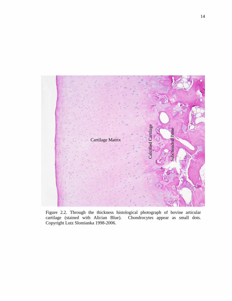

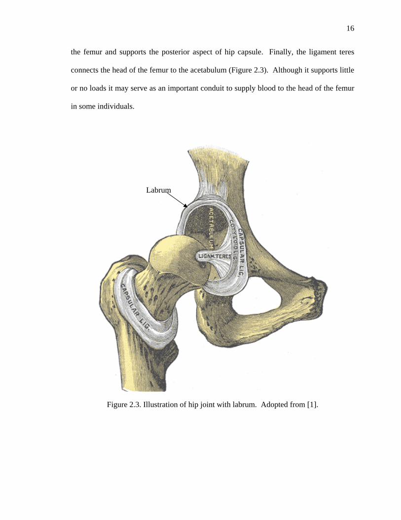


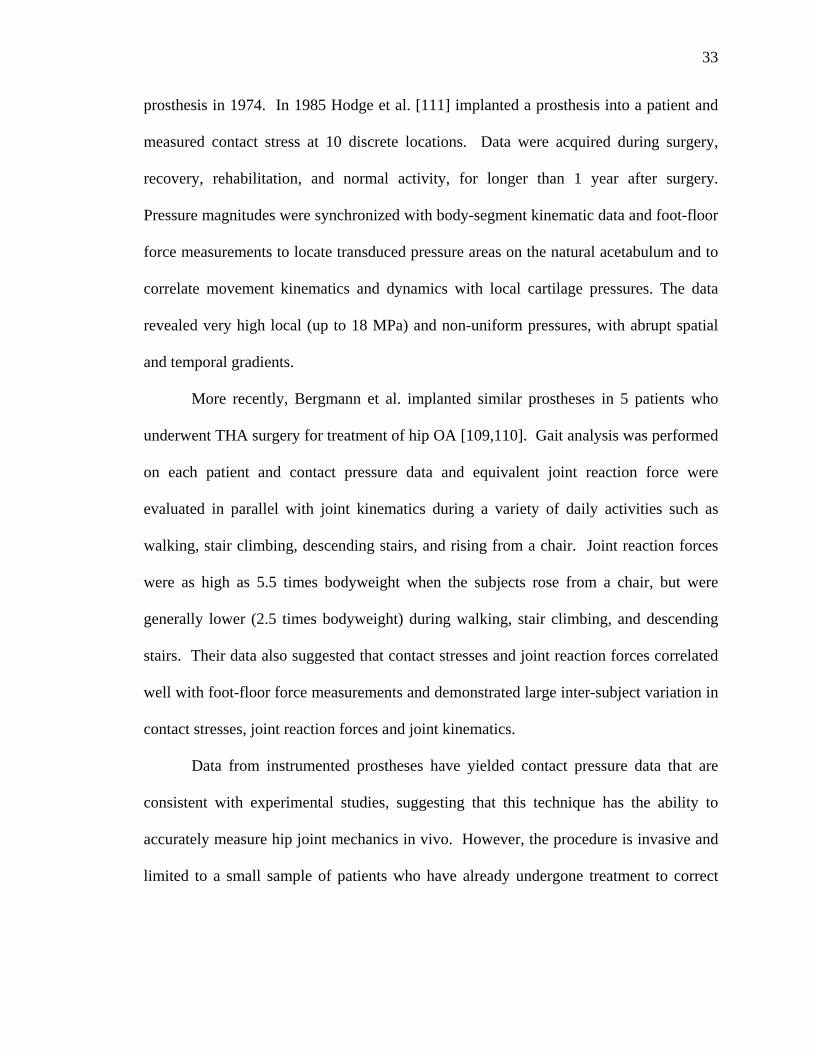


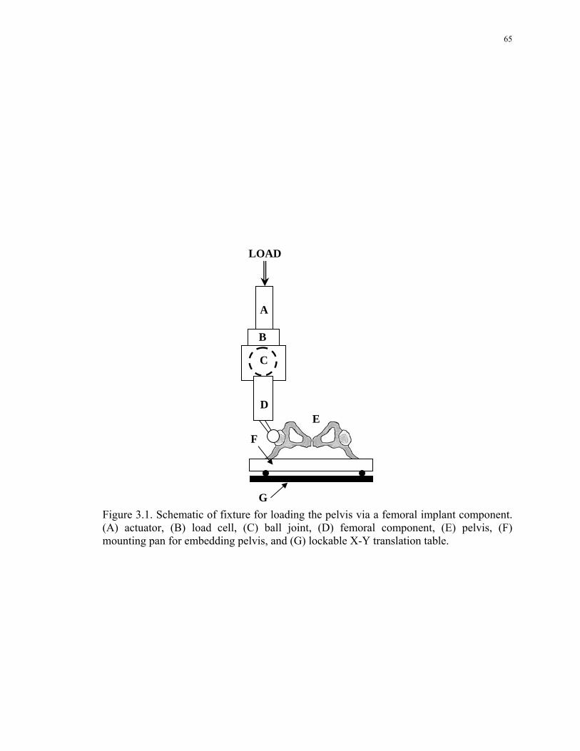


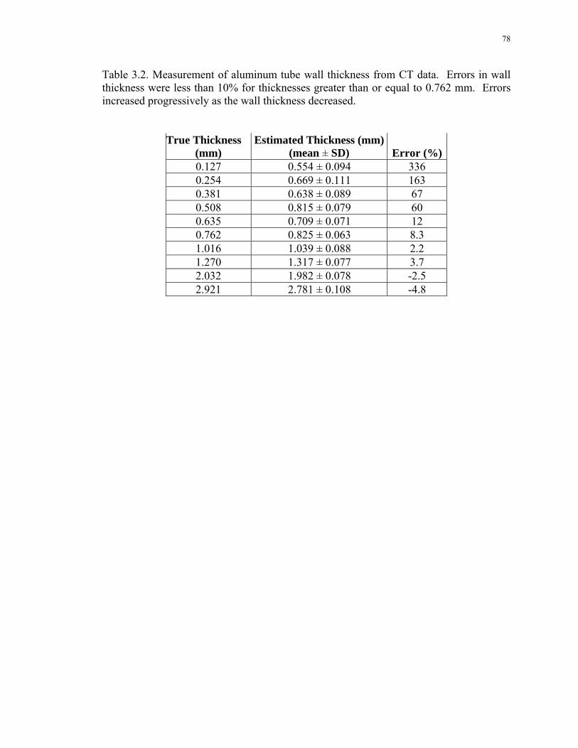


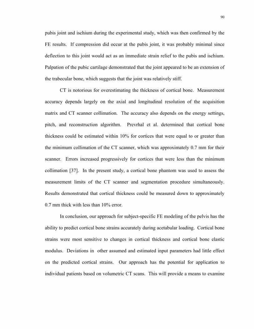


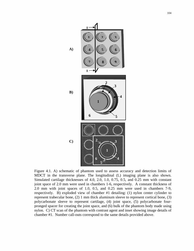


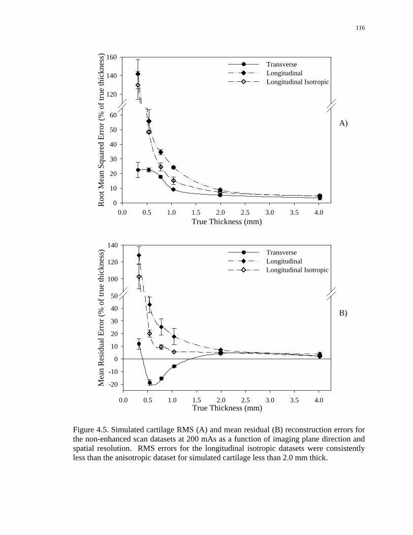


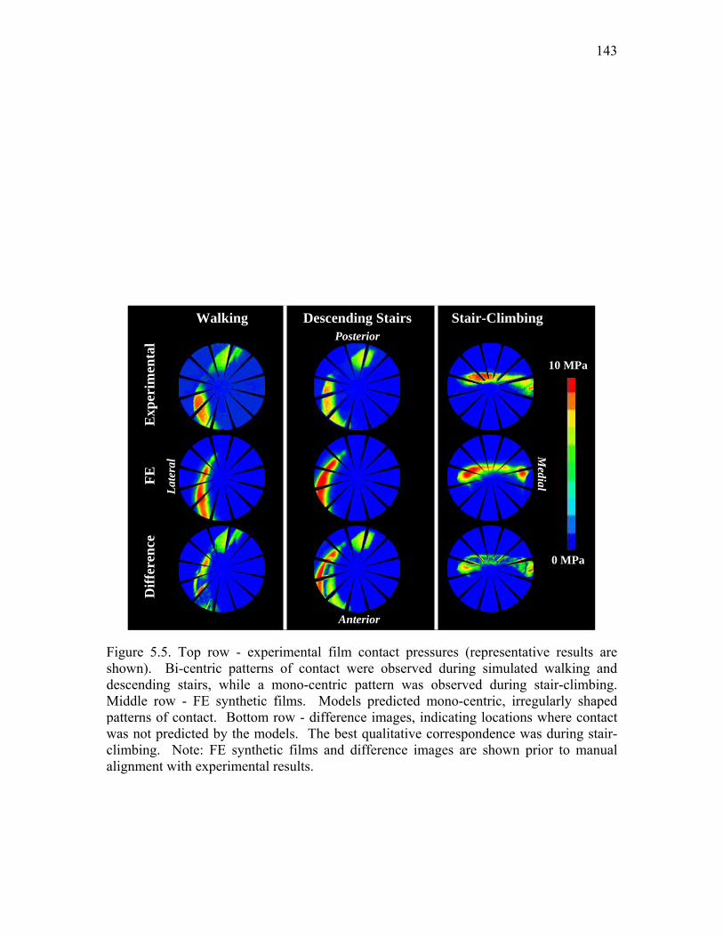


![BUS BUS BUS + + ] ] ] 1 1 1 1 1 1 1 1 1 1 1 1 1 1 1 1 1 1 9 April 2016 Liverpool Street to Colchester, Ipswich, Norwich and branches BUS BUS BUS + +] ] ] 1 1 1 1 1 1 1 1 1 1 1 1 1 1 1 1 1 1 Liverpool Street ...](https://static.documents.pub/doc/80x56/5ab66ff47f8b9a2f438d9b0b/bus-bus-bus-1-1-1-1-1-1-1-1-1-1-1-1-1-1-1-1-1-1-9-april-2016-liverpool.jpg)


![[XLS] Inventory List.xlsxWeb view3 1 2 425 25 1 3 3 1110814715 2 1110813211 2 310816244 1 1 64 37 1 1 1 1 3 1 7 1 1 10 11 4 4 763100386 1 17 4 3 1 2 1 3 7 3063002 1 1 1 1 2 1 41 1 4 3 2 1 1 1 2 1 1 1 8 5 3 2 3 4 2 3 2 1 1 1 1 1 1 1 1 1 2 2 2 2 1 1 1 2 1 1 1 1 1 1](https://static.documents.pub/doc/80x56/5b0810917f8b9a992a8bc102/xls-inventory-listxlsxweb-view3-1-2-425-25-1-3-3-1110814715-2-1110813211-2-310816244.jpg)