Sensitivity of a data-driven soil water balance model to estimatesummer evapotranspiration along a forest chronosequence
J. A. Brena Naranjo, M. Weiler, and K. Stahl
Institute of Hydrology, University of Freiburg, Germany
Received: 16 May 2011 – Published in Hydrol. Earth Syst. Sci. Discuss.: 26 May 2011Revised: 30 October 2011 – Accepted: 2 November 2011 – Published: 17 November 2011
Abstract. The hydrology of ecosystem succession gives riseto new challenges for the analysis and modelling of waterbalance components. Recent large-scale alterations of for-est cover across the globe suggest that a significant portionof new biophysical environments will influence the long-term dynamics and limits of water fluxes compared to pre-succession conditions. This study assesses the estimationof summer evapotranspiration along three FLUXNET sitesat Campbell River, British Columbia, Canada using a data-driven soil water balance model validated by Eddy Covari-ance measurements. It explores the sensitivity of the modelto different forest succession states, a wide range of compu-tational time steps, rooting depths, and canopy interceptioncapacity values. Uncertainty in the measured EC fluxes re-sulting in an energy imbalance was consistent with previousstudies and does not affect the validation of the model. Theagreement between observations and model estimates provesthat the usefulness of the method to predict summer AETover mid- and long-term periods is independent of stand age.However, an optimal combination of the parameters rootingdepth, time step and interception capacity threshold is neededto avoid an underestimation of AET as seen in past studies.The study suggests that summer AET could be estimated andmonitored in many more places than those equipped withEddy Covariance or sap-flow measurements to advance theunderstanding of water balance changes in different succes-sional ecosystems.
Forested ecosystems are strongly subjected to human distur-bances (Bonan, 2008; Hansen et al., 2010) and natural en-vironmental changes (e.g. Kurz et al., 2008). From the year2000 to the year 2005 more than 1 million km2 of global for-est cover was either converted to agricultural land or alteredinto developing successional forests (Hansen et al., 2010).Due to the magnitude of recent large-scale disturbances, thelong-term effects of ecological succession on the exchangesbetween the atmosphere and a recovering biosphere are amajor concern. Studies in temperate and boreal landscapeshave found substantial differences in the carbon cycle (Sitchet al., 2003; Magnani et al., 2007; McMillan et al., 2008)and energy budget (Amiro et al., 2006; Juang et al., 2007) ofdifferently aged forest including post-disturbance forest suc-cession. Forest hydrology studies have long focused on post-disturbance flood increase, but few studies have attempteda quantification of the systematic influence of a recoveringforest on the water balance. Jassal et al. (2009) found thatin a Douglas fir succession initially reduced actual evapo-transpiration (AET) recovered 12 yr after disturbance. BrenaNaranjo et al. (2011) detected a recovery effect on AET inforest chronosequences and on the water balance in variouswatersheds in the North American West. Although changesin AET exhibited a different timing, a gradual recovery wascommon for at least 60 yr after disturbance. The uncertaintyin estimating the timing of such long-time recovery leavesopen questions about the complexity models need to predictannual or seasonal AET in a post-disturbance forest coverscenario.
Micrometeorological data obtained from the Eddy Covari-ance technique (EC) in experimental forested sites that al-low to examine the effects of disturbance and successionon water, energy and biogeochemical fluxes are limited toa few research sites along chronosequences (e.g. Stoy et al.,
Published by Copernicus Publications on behalf of the European Geosciences Union.
3462 J. A. Brena Naranjo: Sensitivity of a data-driven soil water balance model
2006, Jassal et al., 2009). However the scale of disturbancecalls for more research and in particular for better monitor-ing of the water balance. In transitional climate zones suchas those with a Temperate to Mediterranean Climate Typethis research gap concerns particularly the summer AET ofchanging ecosystems.
Current experimental research in forests is characterizedby the holistic observation of the soil-vegetation-atmospherecontinuum. Measurements of water fluxes at the ecosystemscale for modelling purposes are, however, constrained bylimitations at the spatial scale. The high degree of hetero-geneity in soils can significantly affect the dynamics of wa-ter movement between the vadose zone and the atmosphereat large spatial scales. At the plot scale, the approximaterepresentative footprint of the soil moisture measurements isin the order of 100 m2 whereas the usual scale from the ECmeasurements is about 104 m2 (Wilson et al., 2001). Fur-thermore, EC measurements typically underestimate the la-tent heat flux because of a bias in the data acquisition in-struments, neglected energy storage sinks, losses from highfrequency signals and advection (Wilson et al., 2002). Witha lack of energy balance closure between 10 and 30 % thesurface energy imbalance presents considerable uncertainty.This issue is further discussed in Appendix A1. Despite thesechallenges, the comparison between AET derived from soilwater balance methods and EC observations have been pre-viously explored and validated (Wilson et al, 2001; Schumeet al., 2005; Kosugi et al., 2007).
Previous studies using EC observations to validate soil wa-ter budget methods are summarized in Table 1. Although thecharacteristics of each study are quite variable, most of theresults are based on short-term periods or field campaigns,especially during the summer season. While the verticalscale of the observations ranged from 0–100 cm± 40 cm, thenumber of spatial measurements varies from two or three soilwater content probes in semi-arid ecosystems (Scott, 2010)to a maximum of 100 probes in a temperate mixed forest(Schume et al., 2005). Some studies interrupted the soil wa-ter balance computations during rainfall periods as they hadno means to account for wetting front propagation, rechargeand/or due to inadequate turbulent flux measurements (Wil-son et al., 2001; Schelde et al., 2011). Other studies providedAET estimates based on continuous measurements (Cuencaet al., 1997; Moore et al., 2000). Another discrepancy foundwas the time step considered for modeling. As shown in Ta-ble 1 the soil water balance was estimated either using dailytime steps (Cuenca et al., 1997; Wilson et al., 2001; Scheldeet al., 2011) or shorter temporal resolutions (Schume et al.,2005; Schwarzel et al., 2009; Scott, 2010). Even though theresults from the water balance were moderately lower com-pared to the measurements from the EC technique (with theexception of Schume et al., 2005) the rainfall interception bythe canopy was not always explicitly considered in the mod-els (Table 1). Soil water balance models may have additionalreasons to underestimate actual evapotranspiration. These in-
clude the negligence of interception and root water uptake inshallower layers than the actual root zone depth (Table 1).
Although previous studies were successful in validatingthe use of the soil water budget to predict AET, none of themhas examined systematically: (Eq. 1) a wide range of thefew parameters in a data-driven soil water balance model and(Eq. 2) the potential errors arising from computation timesteps. This study aims to explore the sensitivity of a data-driven soil water balance model to estimate summer AETalong a forest chronosequence in a temperate climate. Be-sides testing the sensitivity of the model for different ageforests and to a range of rooting depths and canopy intercep-tion capacity values, we specifically consider the followingquestions: (a) does the model performance depend on thecomputation time step?, (b) how much is the aggregation ofthe computation time step neglecting hydrological processesat the point scale?, and (c) what is the adequate timescale atwhich simple mass-balance approaches can adequately pre-dict AET?
2 Modelling approach and validation
We will test two hypotheses concerning model behaviour.Our first hypothesis is that by choosing small computationtime steps1t , event-based processes affecting the soil waterdepletion from transpiration and soil evaporation and evap-oration from the canopy will be more frequently observedand taken into account in the model. However, as1t be-comes larger, recharge will be explicitly accounted for re-sulting in an underestimation of summer AET. Our secondhypothesis is that a soil water balance will provide better re-sults in younger than in older forested ecosystems as the lackof dense canopy foliage in young stands diminish the role ofinterception while at the same time it enhances soil moisturedepletion through soil evaporation and root water uptake asthe dominant processes in AET. Nevertheless, we acknowl-edge that the canopy interception component in temperateconiferous forests are primarily a function of the frequencyand duration of storms rather than stand structure (Gash andMorton, 1978).
During summer dry periods the soil water balance is pro-portional to the root water uptake and to evaporation fromthe soil. Previous research suggested that soil moisture lim-its evapotranspiration, especially during water stress periods(Teuling et al., 2006a, b). For most forest trees, includingDouglas fir, the majority of roots are within the upper 50 cm,and absorbing roots are in the top 20 cm (Hermann, 1977). Inregions with high rainfall amounts, compacted soil, or poordrainage, roots may be extremely shallow- in the top few cen-timetres only (Helliwell, 1989). This was corroborated byHumphreys et al. (2003) by estimating soil matric potential atthe MS with the support of soil water retention curves whichindicated that the bulk of the roots active in water uptakewere in the upper 30 cm of soil. In this study we consider the
J. A. Brena Naranjo: Sensitivity of a data-driven soil water balance model 3463
Table 1. Previous studies combining soil water balance and EC measurements.
Source Seasons Soil depth Probes Time∗ 1t Model Inter-ception Slope EBR EB# range (cm) /site (%) (h) performance EB gap
Cuenca et al. (1997) 1 0–120 5 0 24 Underest. Yes NAMoore et al. (2000) 2 0–155 NA 0 NA NA Yes 0.91 NA NAWilson et al. (2001) 1 0–70 7 57 24 Underest. No NA NA 0.8Schume et al. (2005) 1 0–100 100 0 0.25 OK No NA NA 0.85Schwarzel et al. (2009) 1 0–90 51 & 64 NA 1 Underest. Yes 0.82–0.87 NA NAScott (2010) 13 0–100 2–3 49 0.5 Underest. No 0.73–0.83 0.96–1.04 NASchelde et al. (2011) 1 0–75 8 47 24 Underest. Yes NA
∗ Amount of time removed because of rainfall and/or flux corrections.
soil moisture dynamics during a summer period of 100 daysfrom the end of June to the beginning of October (DOY 175to 275). Two parsimonious data-driven soil water balancemodels with different complexity were tested across the threedifferently aged stands. In addition to four canopy intercep-tion thresholds described in Sect. 3, six different model timesteps (1t): 30 min, 60 min, 180 min, 360 min, 720 min and1440 min and three different soil depths (Zr): 0–30, 0–60and 0–100 cm were used.
The chosen models do not consider physical and biologicaldrivers of evapotranspiration such as net radiation, vapourpressure deficit, leaf area index and canopy conductance, butassume that the soil water balance can estimate AET duringdry periods by:
Zrdθ(t)
dt= P(t)−q(t)−(Es(t)+T (t)) (1)
whereZr is the active root depth,P is rainfall, q is perco-lation, Es is soil evaporation,T is transpiration andθ is thevolumetric soil water content. With the exception ofZr (inmm) andθ(−), all variables are expressed in mm/1t . Forfurther simplification, we assume that the value ofZr and thesoil depth where soil moisture limitsEs+T is similar.
This simple water balance model may be valid in youngstands where rainfall interception is low. Nevertheless, asforests transition to mature ecosystems, interception willplay an important role in evapotranspiration (e.g. Savenije,2004). A second water balance model (Eq. 2) thereforeadded the evaporation from water stored in the canopyI (t).A maximum canopy interception capacityImax (mm h−1) isdefined to calculate the time variable evaporation from thecanopyI (t) = Imax whenP(t) ≥ Imax andI (t) = P(t) whenP(t) < Imax. The total AET will hence depend on the evapo-ration from canopy:
AET(t) = Es(t)+T (t)+I (t) (2)
Positive values ofdθ(t)dt
due to infiltration and hydraulic re-distribution of soil water were considered to be equivalentto percolationq(t). The model assumes thatq occurs onlyduring rainfall events and up to 2 h after the end of rainfall.During this period we did not calculate AET from the soil
moisture observations. For periods before and after this de-fined period, we assumed thatq is equal zero.
The aggregation of computation time steps from 30 mininto 1, 3, 6, 12 and 24 h implies to sum the fluxes (P , θ ,q, I ) so theI (t) values from low-intensity rainfall events,lower that the canopy interception capacity, are set toImax.Likewise, as the time scale of infiltration and redistributionafter a storm is smaller than the larger1t ’s and for which thesoil water content was averaged over1t values, the impactof summer storms will be implicitly included in the waterbalance calculations with the longer model time step.
For model validation, observed AET from the flux tow-ers was used. To assess sensitivity of the estimates to thedifferent model choices, modelled and observed AET werecompared at two different levels of aggregation:
1. mean total summer AET over the study period
2. mean diurnal cycle.
Furthermore, the sensitivity to the inter-annual climatic vari-ability was assessed based on the total annual summer AETas well as on Nash-Sutcliffe efficiency index (NSE) (Nashand Sutcliffe, 1970) for the simulated time series of eachsummer.
3 Study site
This study used data from an evergreen forest chronose-quence located on the east coast of Vancouver Island, BC,Canada. The Campbell River forest chronosequence, an ex-perimental research site member of the FLUXNET initiative(Baldocchi et al., 2001), consists of three differently agedcoastal Douglas-fir (Pseudotsuga menziesii(Mirbel) Franco)stands: a young (YS), intermediate (IS) and mature stand(MS). Published data available to the scientific communitywas obtained online(http://www.fluxnet-canada.ca/). Thethree sites were harvested in 2000, 1988 and 1949 respec-tively, followed by slash-burning and planting predominantlyDouglas-fir seedlings. Subsequently, several overstory andunderstory species have also grown. The climate at the sites
3464 J. A. Brena Naranjo: Sensitivity of a data-driven soil water balance model
Table 2. Characteristics of the successional forest chronosequence experimental sites in Campbell River, Canada.
Young stand Intermediate stand Mature stand
Abbreviation YS IS MSYear of establishment 2000 1988 1949Latitude 49◦52′20′′ N 49◦31′11′′ N 49◦52′8′′ NLongitude 125◦17′32′′ W 124◦54′6′′ W 125◦20′6′′ WElevation (masl)a 175 170 300Average tree height (m)a 2.4 7.5 33Stand density (trees ha−1)a 1400 1200 1100Mean summer LAI± std. dev (−) 1.9± 0.5b 5.5 to 6.8c 8.4c
Mean annual ET (mm)a 253 362 398Mean summer ET (mm) 126 161 168Mean summerP (mm) 112 121 135
afrom Jassal et al. (2009),bfrom 2002 to 2005,cfrom Humphreys et al. (2000)
is characterized by cool and rainy winters and, dry and rela-tively warm summers. Mean annual precipitation is 1497 mmand the mean annual temperature is 9◦C. The average grow-ing season extends from March to October. From May to Oc-tober the region has climatic moisture deficits with the largestvalues in July and August (Moore et al., 2010). Soil textureat all sites is in the range from gravely loamy sand to sand.Humphreys et al. (2006) and Jassal et al. (2009) describedfurther details about the sites. The main characteristics ofthe forest chronosequence are shown in Table 2.
A meteorological tower sampled the vertical exchangesof latent heatλE above each stand using the EC technique.Half-hourly fluxes of water vapour were provided from three-axis anemometers and infrared gas analysers (for more de-tails see Jassal et al., 2009). The quality of the turbulentfluxes at the three sites was not affected by the wind direc-tion and the energy balance closure did not decrease whenwind came from behind each EC tower (Humphreys et al.,2005). Moreover, specific wind directions were not used toremove observed fluxes given the sufficient area of homoge-neous stand footprint were within the typical values. At theMS, the fetch was 400 m to the southwest and about 700 to800 m to the northeast with Douglas fir stands between 25 to60 yr old surrounding the tower from all sides (Humphreyset al., 2003). At the IS, the fetch was between 400 and700 m in all directions and surrounded by young and matureforests. At the YS, the fetch was about 400 m in both thenortheast and southwest directions surrounded in all direc-tions by 60 yr-old Douglas-fir forests. Footprint assessmentssuggested that the minimum fetch estimated for all the siteswas sufficient for flux observations (Humphreys et al., 2006).Humphreys et al. (2003) established that anabatic–katabaticcirculation patterns occurring during most of the year couldreduce the expected generation of local circulations patternsdeveloped by the thermal convection due to clear-cut areas
surrounded by mature forests. The quality control proce-dures of measured latent heat fluxes involved despiking, es-pecially during periods of heavy rainfall, and removing por-tions of the high frequency time series associated with cal-ibrations before computing EC statistics (Humphreys et al.,2006). Fluxes with statistics that did not fall within reason-able limits and/or occurred during instrument malfunctionwere removed. Flux measurements were also removed whendata did not fall within the specified limits for realistic data,when the water vapour mixing ratio was negative and whenthe non-stationarity ratio was greater than 3.5 (Mahrt, 1998).The underestimation inλE ranged from 0 to 10 %. AnymissingλE measurements were replaced using the Penman-Monteith equation. Observed weather variables and canopyconductance were modelled using a Jarvis-Stewart parame-terization (see Humphreys et al., 2003).
Precipitation (P ) was measured in each stand using twotipping-bucket rain gauges. The frequency of the observa-tions was recorded at 3 s intervals and then averaged for30 min (model 2501 tipping bucket rain gauge, Sierra Misco,Berkeley, CA or model 4000 Jarek Manufacturing Ltd.,Sooke, BC, Canada). In order to avoid outliers, the precipita-tion records at the MS site and at the nearby Campbell RiverAirport, British Columbia were compared and considered ac-ceptable since the difference in total rainfall recorded at thetwo locations within the summer months was less than 5 %(Humphreys et al., 2003). Precipitation data were gap-filledusing statistical relationships with related data from the samesite or the other sites(http://fluxnet.ccrp.ec.gc.ca). Errors de-rived from wind factors (gage setup, wind speed and dropsize distribution) were not accounted. Scott (2010) foundan underestimation of 5 % for semi-arid ecosystems with anannualP between 280 and 400 mm. The summer precipita-tion across our the study site varied from less than 100 mmto more than 200 mm in dry and wet summers, respectively.
J. A. Brena Naranjo: Sensitivity of a data-driven soil water balance model 3465
Wind during the summer period is relative low compared tothe winter. Therefore we expect an overall error for precipi-tation during summer in the range of 2–5 %.
Percolation (q) was not measured. However volumetricsoil water content data (θ ) were available from two loca-tions at each site equipped with time-domain reflectometry(TDR) probes reporting depth ranges averaged over 0–30, 0–60 and 0–100 cm with a time resolution of 30 min (Jassal etal., 2009). Moreover, 11 additional TDR sensors integratingthe top 30 and 76 cm of the soil profile were manually mea-sured monthly with a cable length tester and used to observethe spatial variability inθ over the turbulent flux source areaat the MS (Humphreys et al., 2003). The probes were estab-lished below ground level and beneath the organic layers ofleaf litter, near the tower/hut. The high-resolution data fromthe two locations was averaged and then used as the modelinput. The original EC andθ data were screened for instru-ment failure and gap-filled (Humphreys et al., 2005, Jassal etal., 2009).
Humphreys et al (2003) estimated canopy interceptionwith two methods. The first method used measured through-fall and stemflow rates at the MS site. In addition, a secondmethod with the support six leaf wetness sensors was used todetermine the minimum depth of water required to saturatethe entire canopy surface (1.5 mm), or canopy interceptioncapacity (Imax) (Leyton et al., 1965) at different heights ofthe MS canopy. The canopy was assumed to be completelywet when all the leaf wetness sensors were wet or the cal-culated water stored on the canopy was greater than 1.5 mm.The canopy was assumed to be dry when all the leaf wetnesssensors were dry and the water stored on the canopy was0 mm. The degree of uncertainty was large, the agreementbetween estimates of the canopy wetness and, the canopyinterception capacity inferred from the sum of throughfalland stemflow ranged between 50 and 70 % (Humphreys etal., 2003). Moreover, the maximum threshold ofImax wasroughly approximated from the observed daily AET at the3 stands before the energy balance closure. The daily AETvaried from 2.5 mm to less than 1 mm day−1 at the early andlate stages of the summer season, respectively.
Based on these observations,Imax is considered not to belarger than 1 mm h−1. Because of differences in LAI, the sen-sitivity analysis in this study tested values ofImax of 0.25, 0.5and 1 mm h. Such values also fit with the interception thresh-old of 0.5 mm h−1 suggested by Gash (1979). The valueof Imax assumed that the water falling on the canopy dur-ing low-intensity rainfall intensity events (up toImax) willmostly be stored and evaporate. Rainfall intensities exceed-ing this threshold will cause throughfall to the soil surfaceand infiltration into the soil. Jassal et al. (2009) providesLAI data measured during the summer season in 2002–2005at the young stand and in 2002 at the intermediate/maturestands. The LAI variability observed for the mentioned peri-ods was not expected to change theImax range of values. Thedata is shown in Table 2. The mean annual energy balance
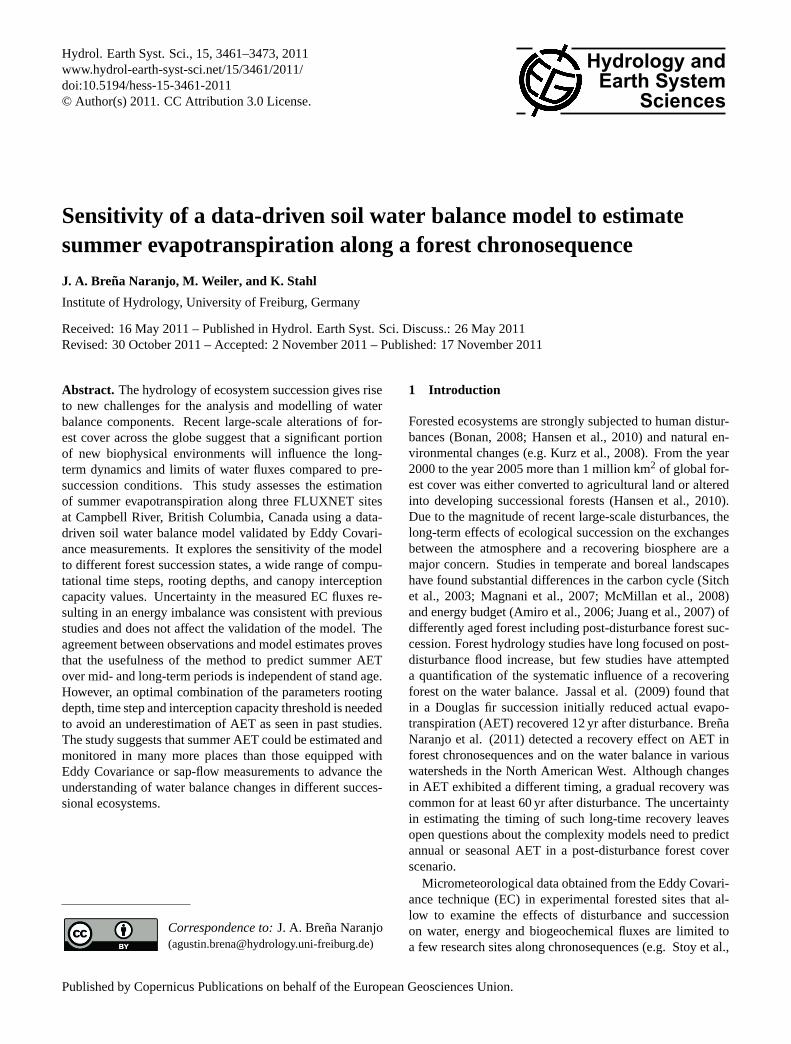
Fig. 1. Measured time series of precipitation (cumulative), evapo-transpiration (cumulative) and soil moisture during a dry summer(2003,a andb) and a wet summer (2004,c andd) at the maturestand (MS).
closure at the YS, IS and MS was 0.89, 0.83 and 0.88, respec-tively (Jassal et al., 2009). Our study period covered sevensummer seasons at the young and mature stands from June2001 to September 2008. Observations at the intermediatestand began in 2002.
An example of the water supply-demand in this study siteduring periods of different water-stress and the importanceof the soil water reservoir is shown in Fig. 1. Within thesame stand (MS), summer AET will be about 150 mm ina dry summer following a dry winter (Fig. 1a) and about170 mm in a wet summer (Fig. 1c). While the differencein AET between such contrasting summer seasons in about20 mm,P in the wet summer was twice as much as in thedry summer. In such cases, the soil water deficit from scarcesummer rainfall and water use by vegetation will be compen-sated by soil moisture stored during spring and winter (Fig. 4,top). Figure 1b, d show the vertical distribution of soil watercontent for the same contrasting summers. During dry sum-mers (Fig. 1b), the soil water content at shallow soil layersis rapidly depleted compared with the deeper layers whereasthis pattern changes at the end of the summer or during wetsummers (Fig. 1d).
4 Results
4.1 Sensitivity of the model
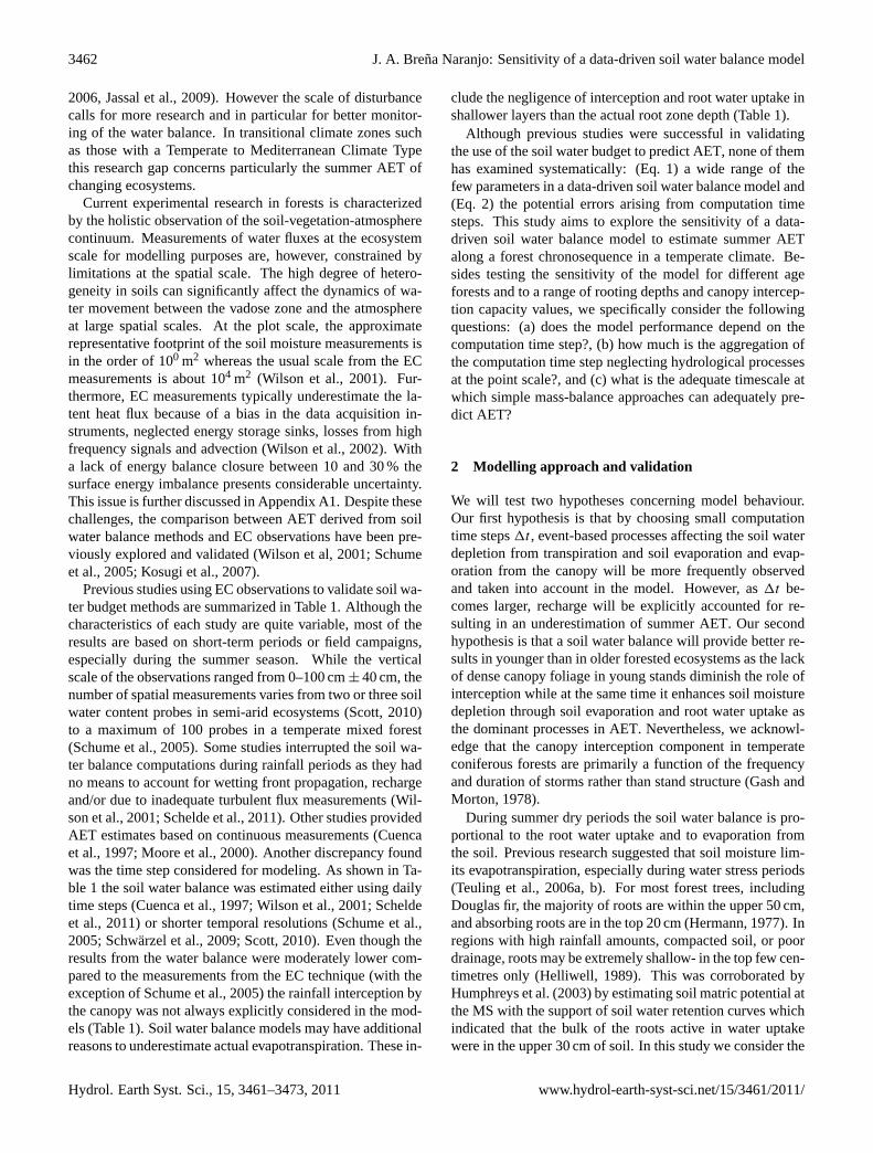
Figure 2 (top) shows the mean diurnal cycle of observed andsimulated summer AET from 2001 to 2008 usingZr = 30 cm,Imax= 0.25 mm h−1 and1t = 60 min. AET is generally un-derestimated during daytime: slightly at the young stand
3466 J. A. Brena Naranjo: Sensitivity of a data-driven soil water balance model
Fig. 2. Modeled and observed summer AET (2001–2008) based onZr = 30 cm,Imax= 0.25 mm h−1 and1t = 60 min: (top) mean diurnalcycle simulated (middle) mean daily AET values simulated (bottom) mean hourly AET values simulated (zoomed in from the whole timeseries).
(YS) and mature stand (MS), but strongly at the intermedi-ate stand (IS). AET is overestimated during nighttime, againmost strongly at IS, where the AET observations show aweaker diurnal variation than at the other stands. With theexception of the YS, the observed soil moisture depletionduring nighttime does not reflect the observed strong reduc-tion of latent heat fluxes during the night using EC.
Using the same modeling time step of1t = 60 min, Fig. 2(middle) shows the observed and simulated mean daily sum-mer AET from 2001 to 2008. AET is strongly underes-timated in early to mid summer and slighty overestimatedin late summer. Daily AET at IS and MS is overestimatedslightly more during the second half of the summer periodwhen autumn storms start to occur. For all sites, the esti-mated mean daily AET in the second half remains relativelyconstant whereas the measurements indicate a decrease. Fi-nally, the mean AET at each hourly time step (Fig. 2, bottom)shows the main weakness of the soil water balance model,which estimates significantly higher or lower values at cer-tain time steps.
Table 3 shows the sensitivity analysis of the model to amultiple combination of rooting depth (Zr) and canopy in-terception capacity values (Imax) for a fixed time step of1t = 30 min. The errors were calculated for the mean to-tal summer AET for the period 2001 to 2008. The resultsare acceptable when the soil moisture dynamics are consid-ered in the shallow soil layer of 0–30 cm. As the rootingdepth is assumed to be larger (e.g. 60 cm and 100 cm), the
depletion of the volume of soil water within the layer tendedto overestimate summer AET. An exception was observedat the intermediate stand for moderate and highImax. Thesensitivity of the model toImax was rather heterogeneous.The differences in the absolute error fromImax= 0 mm h−1
to Imax= 1 mm h−1 were lower for YS than for IS and MS.When the error was expressed relative to the observed AETthe differences between YS, IS, and MS are not as pro-nounced.
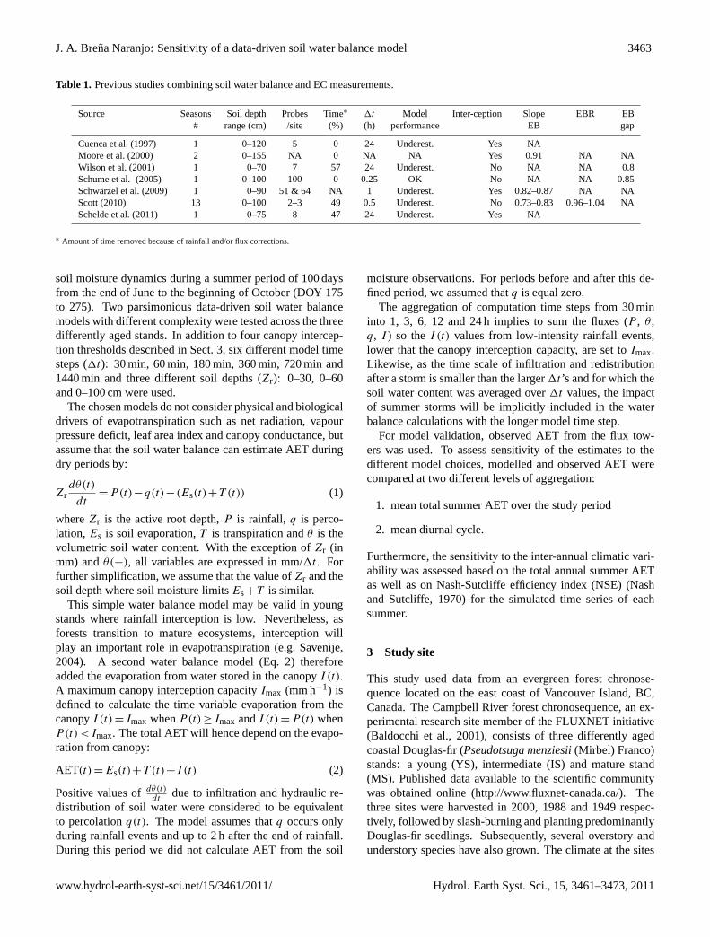
The sensitivity to the computational time step is shownin Table 4 and Fig. 3. Overall, the absolute and relative er-rors increased whereas the NSE decreased as the soil mois-ture data was aggregated over longer time steps. The step1t = 30 min provided the best results for the YS and IS but1t = 60 min proved to be more adequate for the MS. De-spite an overall decay of model performance as a function ofthe time step (Fig. 3), an example of model equifinality (i.e.same results with different model parameters) was observedat the YS when a similar error was obtained for1t =30 minand 180 min (Table 4). The main difference in the parametercombination was found to beZr = 30 cm for1t = 30 min andZr = 60 cm for1t = 180 min. Finally, the differences in theerror for the least optimal1t = 1440 min (= 24 h) at the threestands differed strongly. The largest error was observed atthe IS followed by the YS and the MS. Stand age was not animportant factor affecting model performance, but its sensi-tivity to the time step.
J. A. Brena Naranjo: Sensitivity of a data-driven soil water balance model 3467
Table 3. The sensitivity of the model to soil depth, canopy interception and a fixed1t = 30 min. The sensitivity is expressed as the absoluteerror (AE), relative error (RE) and Nash-Sutcliffe efficiency index from the mean total summer AET (mm) for the period 2001–2008. Thelowest errors in each stand are highlighted in bold. Uncertainty derived from the energy imbalance is not considered.
Young stand (YS) Intermediate stand (IS) Mature stand (MS)
Zr Imax AE RE NSE AE RE NSE AE RE NSE(cm) (mm h−1) (mm) (%) (−) (mm) (%) (−) (mm) (%) (−)
100 0.0 NA NA NA NA NA NA +127 +80 −0.910.25 NA NA NA NA NA NA +137 +95 −0.90.5 NA NA NA NA NA NA +157 +97 −1.221.0 NA NA NA NA NA NA +165 +102 −1.42
Fig. 3. Sensitivity of the data-driven soil water balance model tothe computational time step (1t). The relative error shown is thelowest error obtained by the combination ofZr andImax for eachtime step.
4.2 Interannual variability
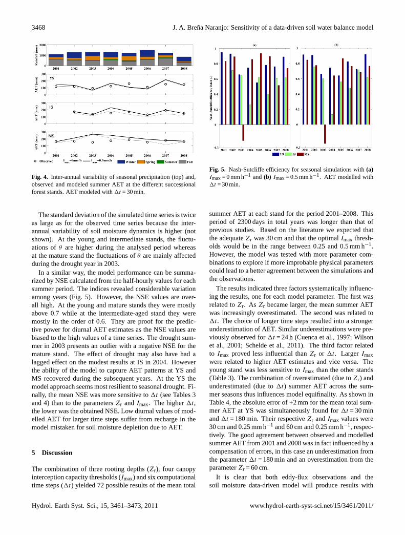
Observed summer AET shows considerable inter-annualvariability with differences along the chronosequence: AETat the YS and IS generally varies more from year to year thanAET at the MS (Fig. 4). For the different stands the perfor-mance of the model of each summer shows a different sen-sitivity to this climatic variability (Fig. 5). The summers in2003 and 2006 were dry compared to historical observations
Table 4. Sensitivity of the data-driven soil water balance modelto the computational time step (1t). The absolute error and NSEshown is the lowest obtained by the combination ofZr andImax foreach time step. The relative error is shown in Fig. 3. The absoluteerror (AE) after the correction from the slope of the energy balanceis shown in brackets.
while 2004 and 2007 were wet summers. Figure 4 shows thatthe observed AET in those years and the simulatedEs+T
(dashed line) at the YS and IS followed the expected vari-ation of ET from a dry to a wet summer and subsequentlyto a dry one. The behaviour at the MS was more complex.The soil water balance indicates an increase inEs+T untilthe occurrence of the extreme dry summer of 2003 and thenstarted a steady decrease until 2008 despite the subsequentwet summers. The inclusion of evaporation fromI (t) (boldline) has hardly any effect on the magnitude and interannualvariability of AET at the YS. However, at the IS the inclusionof I (t) improved the prediction of AET during five years outof six.
3468 J. A. Brena Naranjo: Sensitivity of a data-driven soil water balance model
Fig. 4. Inter-annual variability of seasonal precipitation (top) and,observed and modeled summer AET at the different successionalforest stands. AET modeled with1t = 30 min.
The standard deviation of the simulated time series is twiceas large as for the observed time series because the inter-annual variability of soil moisture dynamics is higher (notshown). At the young and intermediate stands, the fluctu-ations ofθ are higher during the analysed period whereasat the mature stand the fluctuations ofθ are mainly affectedduring the drought year in 2003.
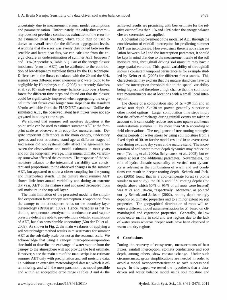
In a similar way, the model performance can be summa-rized by NSE calculated from the half-hourly values for eachsummer period. The indices revealed considerable variationamong years (Fig. 5). However, the NSE values are over-all high. At the young and mature stands they were mostlyabove 0.7 while at the intermediate-aged stand they weremostly in the order of 0.6. They are proof for the predic-tive power for diurnal AET estimates as the NSE values arebiased to the high values of a time series. The drought sum-mer in 2003 presents an outlier with a negative NSE for themature stand. The effect of drought may also have had alagged effect on the modest results at IS in 2004. Howeverthe ability of the model to capture AET patterns at YS andMS recovered during the subsequent years. At the YS themodel approach seems most resilient to seasonal drought. Fi-nally, the mean NSE was more sensitive to1t (see Tables 3and 4) than to the parametersZr andImax. The higher1t ,the lower was the obtained NSE. Low diurnal values of mod-elled AET for larger time steps suffer from recharge in themodel mistaken for soil moisture depletion due to AET.
5 Discussion
The combination of three rooting depths (Zr), four canopyinterception capacity thresholds (Imax) and six computationaltime steps (1t) yielded 72 possible results of the mean total
Fig. 5. Nash-Sutcliffe efficiency for seasonal simulations with(a)Imax= 0 mm h−1 and(b) Imax= 0.5 mm h−1. AET modelled with1t = 30 min.
summer AET at each stand for the period 2001–2008. Thisperiod of 2300 days in total years was longer than that ofprevious studies. Based on the literature we expected thatthe adequateZr was 30 cm and that the optimalImax thresh-olds would be in the range between 0.25 and 0.5 mm h−1.However, the model was tested with more parameter com-binations to explore if more improbable physical parameterscould lead to a better agreement between the simulations andthe observations.
The results indicated three factors systematically influenc-ing the results, one for each model parameter. The first wasrelated toZr. As Zr became larger, the mean summer AETwas increasingly overestimated. The second was related to1t . The choice of longer time steps resulted into a strongerunderestimation of AET. Similar underestimations were pre-viously observed for1t = 24 h (Cuenca et al., 1997; Wilsonet al., 2001; Schelde et al., 2011). The third factor relatedto Imax proved less influential thanZr or 1t . LargerImaxwere related to higher AET estimates and vice versa. Theyoung stand was less sensitive toImax than the other stands(Table 3). The combination of overestimated (due toZr) andunderestimated (due to1t) summer AET across the sum-mer seasons thus influences model equifinality. As shown inTable 4, the absolute error of +2 mm for the mean total sum-mer AET at YS was simultaneously found for1t = 30 minand1t = 180 min. Their respectiveZr andImax values were30 cm and 0.25 mm h−1 and 60 cm and 0.25 mm h−1, respec-tively. The good agreement between observed and modelledsummer AET from 2001 and 2008 was in fact influenced by acompensation of errors, in this case an underestimation fromthe parameter1t = 180 min and an overestimation from theparameterZr = 60 cm.
It is clear that both eddy-flux observations and thesoil moisture data-driven model will produce results with
J. A. Brena Naranjo: Sensitivity of a data-driven soil water balance model 3469
uncertainty due to measurement errors, model assumptionsand parameterization. Unfortunately, the eddy-flux commu-nity does not provide a continuous estimation of the error forthe estimated latent heat flux, which could then be used toderive an overall error for the different aggregation levels.Assuming that the error was evenly distributed between thesensible and latent heat flux, we can calculate from the en-ergy closure an underestimation of summer AET between 7and 13 % (Appendix A, Table A1). Part of the energy closureimbalance (error in AET) can be attributed to the contribu-tion of low-frequency turbulent fluxes by the EC technique.Differences in the fluxes calculated with the 20 and the 8 Hzsignals (from different sonic anemometers) were found to benegligible by Humphreys et al. (2005) but recently Sanchezet al. (2010) analysed the energy balance ratio over a borealforest for different time steps and found out that the closurecould be significantly improved when aggregating the origi-nal turbulent fluxes over longer time steps than the standard30 min available from the FLUXNET database. Unlike thesimulated AET, the observed latent heat fluxes were not ag-gregated into larger time steps.
We showed that summer soil moisture depletion at thepoint scale can be used to estimate summer AET at the foot-print scale as observed with eddy-flux measurements. De-spite important differences in the main canopy, understoryspecies and root structure, stand age at different stages ofsuccession did not systematically affect the agreement be-tween the observations and model estimates in most yearsand for the long-term average. Interannual climatic variabil-ity somewhat affected the estimates. The response of the soilmoisture balance to the interannual variability was consis-tent and proportional to the observed changes in the summerAET, but appeared to show a closer coupling for the youngand intermediate stands. In the mature stand summer AETshows little inter-annual variability and during an extremedry year, AET of the mature stand appeared decoupled fromsoil moisture in the top soil layer.
The main limitation of the presented model is the simpli-fied evaporation from canopy interception. Evaporation fromthe canopy to the atmosphere relies on the boundary-layermeteorology (Brutsaert, 1982). Hence, variables as net ra-diation, temperature aerodynamic conductance and vapourpressure deficit are able to provide more detailed simulationsof AET, but also considerable uncertainty (Van der Tol et al.,2009). As shown in Fig. 2, the main weakness of applying asoil water budget method results in misestimates for summerAET at the sub-daily scale but not at the seasonal scale. Weacknowledge that using a canopy interception-evaporationthreshold to describe the exchange of water vapour from thecanopy to the atmosphere will not provide the best estimate.However, since the main aim of the manuscript is to estimatesummer AET only with precipitation and soil moisture data,i.e. without an extensive meteorological dataset, which is of-ten missing, and with the most parsimonious model possibleand within an acceptable error range (Tables 3 and 4) the
achieved results are promising with best estimate for the rel-ative error of less than 1 % and 10 % when the energy balanceclosure correction was applied.
A potential improvement of the modelled AET through theconsideration of rainfall interception for predicting summerAET was inconclusive. However, since there is not a clear re-lation between LAI and the interception parameter, it shouldbe kept in mind that due to the measurement scale of the soilmoisture data, throughfall driving soil moisture may have alarge spatial variation. This spatial variability of throughfallshows a consistent temporal persistence as for example stud-ied by Keim et al. (2005) for different forest stands. Thischaracteristic may explain that the mature stand can have thesmallest interception threshold due to the spatial variabilitybeing highest and therefore a high chance that the soil mois-ture measurements are at locations with a small local inter-ception.
The choice of a computation step of1t = 30 min and anactive root depthZr = 30 cm proved generally superior toother model options. Larger computation time steps implythat the effects of recharge during rainfall events are taken inaccount so it can notably reduce root water uptake and henceunderestimate summer ET by more than 50 % according tofield observations. The negligence of tree rooting strategiesduring periods of water stress by using soil moisture from afixed depth of 30 cm for the model resulted in an overestima-tion during extreme dry years at the mature stand. The incor-poration of soil water to root depth dynamics may reduce theerror (Teuling et al., 2006a; Schymanski et al., 2008), but re-quires at least one additional parameter. Nevertheless, therole of hydro-climatic seasonality on vertical root dynam-ics is relevant as the combination of warm and wet condi-tions can result in deeper rooting depth. Schenk and Jack-son (2005) found that in a cool-temperate forest (a biomesimilar to our study), the 50 % and 95 % rooting depths (thedepths above which 50 % or 95 % of all roots were located)was at 21 and 104 cm, respectively. Moreover, as pointedout by Schenk and Jackson (2002), rooting depth stronglydepends on climatic properties and to a minor extent on soilproperties. The geographical distribution of roots will re-quire a different model parameterization forZr based on cli-matological and vegetation properties. Generally, shallowroots occur mainly in cold and wet regions due to the lackof water stress whereas deeper roots have been observed inwarm and dry regions.
6 Conclusions
During the recovery of ecosystems, measurements of heatfluxes, rainfall interception, stomata conductance and rootdepth, among others, show constant change. Under suchcircumstances, gross simplifications are needed in order toavoid a model over-parameterization at each successionalstage. In this paper, we tested the hypothesis that a data-driven soil water balance model using soil moisture and
3470 J. A. Brena Naranjo: Sensitivity of a data-driven soil water balance model
precipitation measurements can provide a reasonable approx-imation of summer AET when choosing an appropriate com-putational time step, rooting depth and canopy interception.The model was validated in a successional chronosequencecharacterized by long-term physiological changes that di-rectly affect the water balance partition in forests. We foundthat stand age does not affect the performance of the model.
The parsimonious data-driven model for the estimationof summer AET presented here has a main advantage overmore data-intensive modelling schemes to study hydrologi-cal changes in recovering forested ecosystems. For exam-ple, LAI, soil properties, boundary-layer meteorology anddetailed root depth parameterization are not required. Thecurrent approach proved to be useful for predicting evapo-transpiration during the water limited period of the year in adisturbed and successional temperate ecosystem and its dif-ferences in their magnitude caused by different patterns ofinterception, soil evaporation and transpiration. An eight-year comparison of both models’ output showed that in orderto provide acceptable AET estimates it is essential to accountfor rainfall in the soil water balance by choosing an adequatecalculation time step (1t) and rooting depth (Zr). However,we would like to emphasize that methods solely based on va-dose zone measurements cannot capture detailed processesoccurring at the vegetation-atmosphere continuum and there-fore are not suitable to describe AET at temporal resolutionsshorter than several days. The model showed to be less sen-sitive to the canopy interception threshold (Imax) than to theformer parameters. Overall, the combination of a1t be-tween 30 and 60 min and aZr between 0 and 30 cm providedthe best estimates for AET. Parameter values outside this op-timal range were likely to enhance error estimates leading toan over- or under-estimation of the summer AET. Accept-able errors using non-optimal parameters were observed butit was found to be the consequence of error compensationfrom the sum of over- and under-estimated periods. The errormeasurements derived from the energy balance non-closuredid not considerably affect the agreement between observedand simulated mean summer AET.
The results provided here showed that one single modelstructure can be sufficient to make an appropriate estimationof hydrologic change in a gradually evolving landscape andthus does not constitute a problem for modelling of transienthydrological systems. However, the model should be testedacross a wide range of forested and non-forested landscapesin different climates to evaluate applications including esti-mates at sites where Eddy Covariance measurements are lim-ited or difficult due to topographic complexity and in siteswhere long-term soil moisture data are available.
Table A1. Parameters of the linear regression between the availableenergy (Rn−G−Sb−SLE−SH ) and the turbulent fluxes (LE +H )at the three stands from 2001 to 2008.
Any model for prediction purposes relies on good quality in-put data. The validation of any model further relies on thequality of the measurements it is validated against. In thiscase, the model validation is affected by the energy balanceclosure of the EC derived AET observations. It is known thatthe EC technique overestimates the available energy and un-derestimates the turbulent fluxes and therefore AET (Wilsonet al., 2002). The energy imbalance also depends on localfactors such as topography, wind direction and friction veloc-ity, among others. In order to estimate the uncertainty in theobserved AET, the surface energy imbalance was estimatedusing two different methods following Wilson et al. (2002):the first is the Energy Balance Ratio (EBR) (Sanchez et al.,2010) over a certain time period. EBR is defined as the ratioof the available energy to the turbulent fluxes:
EBR=Rn−G−Sb−SLE −SH
LE+H(A1)
whereRn is the net radiation,G is the soil heat flux,Sb isthe biomass heat storage flux, SLE is the latent heat storageflux, SH is the sensible heat storage flux, LE is the latent heatflux above the canopy andH the sensible heat flux above thecanopy. All the units are expressed in W m2. The secondmethod used to estimate the lack of closure of the energybalance is an ordinary linear regression between the availableenergy and turbulent fluxes, numerator and denominator inEq. (A1), respectively.
Since the energy imbalance is larger during nocturnal pe-riods (Wilson et al., 2002), the EBR and the linear regressionparameters (slope, intercept,R2 and root mean square error)were estimated for 24 h periods as well as during the day(Table A1). Figure A1 shows the results for the EBR and lin-ear regression. With ERB between 0.71 and 0.85, slopes be-tween 0.75 and 0.85, andR2 between 0.84 and 0.95, the en-ergy imbalance values for the three stands are consistent withprevious studies (Wilson et al., 2002, Sanchez et al., 2010).The IS was the site with the lowest imbalance, the YS rankssecond. The imbalance is larger at the MS. The improvement
J. A. Brena Naranjo: Sensitivity of a data-driven soil water balance model 3471
Fig. A1. Left side: relationship between the measured turbulent fluxes (y-axis) and the available energy (x-axis) at the three stands YS (top),IS (middle) and MS (bottom) from 2001 to 2008. Right side: variability of the average energy balance ratio during the day.
of the closure when excluding the late evening/nocturnal pe-riods (Fig. A1, right side) was moderate at the IS and MS butdid not have any effect at the YS (Table A1).
Acknowledgements.The first author was supported by a schol-arship from the Graduate School of the Faculty of Forestry andEnvironmental Sciences of the University of Freiburg and theLandesgraduiertenforderung Baden-Wurttemberg. The authorsthank Andy Black and his BIOMET research group at the Uni-versity of British Columbia, Vancouver, Canada, for sharing thedata of the Canadian Carbon Program as well as the editor andthree anonymous reviewers for their constructive comments thathave greatly improved the quality of this paper. The GermanResearch Foundation (DFG) open access publication fund coveredthe publication costs.
Edited by: E. Zehe
References
Amiro, B. D., Orchansky, A. L., Barr, A. G., Black, T. A., Cham-bers, S. D., Chapin III, F. S., Goulden, M. L., Litvak, M., Liu, H.P., McCaughey, J. H., McMillan, A., and Randerson, J. T.: Theeffect of postfire stand age on the boreal forest energy balance,Agr. Forest Meteorol., 140, 41–50, 2006.
Baldocchi, D. D., Falge, E., Gu, L. H.,Olson, R., Hollinger, D.,Running, S., Anthoni, P., Bernhofer, C., Davis, K., Evans, R.,Fuentes, J., Goldstein, A., Katul, G., Law, B., Lee, X. H., Malhi,Y., Meyers, T., Munger, W., Oechel, W., Pilegaard, K., Schmid,H. P., Valentini, R., Verma, S., Vesala, T., Wilson, K., and Wofsy,
S.: Fluxnet: A new tool to study the temporal and spatial variabil-ity of ecosystem-scale carbon dioxide, water vapor, and energyflux densities, B. Am. Meteorol. Soc., 82, 2415–2434, 2001.
Bonan, G. B.: Forests and Climate Change: Forcings, Feedbacks,and the Climate Benefits of Forests, Science, 320, 1444–1449,doi:10.1126/science.1155121, 2008
Brena Naranjo, J. A., Stahl, K. and Weiler, M.: Evapotran-spiration and land cover transitions: long term watershedresponse in recovering forested ecosystems, Ecohydrology,doi:10.1002/eco.256, in preparation, 2011.
Brutsaert W.: Evaporation into the atmosphere, Reidel, Dordrecht,The Netherlands, 299 pp., 1982.
Cuenca, R., Stangel, D. and Kelly, S.: Soil water balance in a borealforest, J. Geophys. Res., 102, 29355–29365, 1997.
Gash, J. H. C.: An analytical model of rainfall interception byforests, Q. J. R. Meteorol. Soc., 105, 43–55, 1979.
Gash, J. H. C. and Morton, A. J.: An application of the Rutter modelto the estimation of the interception loss from Thetford forest, J.Hydrol, 38, 49–58, 1978.
Hansen, M. C., Stehman, S. V., and Potapov, P. V.: Quantificationof global forest cover loss, P. Natl. Acad. Sci. USA, 107, 8650–8655, 2010.
Helliwell, D. R.: Tree roots and the stability of trees, ArboriculturalJournal, 13, 243–248, 1989
Hermann, R. K.: Growth and production of tree roots: A review, in:The below ground ecosystem: A synthesis of plant – associatedprocesses, edited by: Marshall, J. K., Range, Colorado: ScienceDept Series No 26, Colorado State University, Fort Collins, 7–28, 1977
Humphreys, E. R., Black, T. A., Ethier, G. J., Drewitt, G. B., Spit-
3472 J. A. Brena Naranjo: Sensitivity of a data-driven soil water balance model
tlehouse, D. L., Jork, E. M., Nesic, Z., Livingstone, N. J.: Annualand seasonal variability of sensible and latent heat fluxes above acoastal Douglas-fir forest, British Columbia, Canada, Agr. ForestMeteorol, 115, 109–125, 2003.
Humphreys, E. R., Black, T. A., Morgenstern, K., Li, Z., andNesic, Z.: Net ecosystem production of a Douglas-fir stand forthree years following clearcut harvesting, Glob. Change Biol.,11, 450–464, 2005.
Humphreys, E. R., Black, T. A., Morgenstern, K., Cai, T. B.,Drewitt, G. B., Nesic, Z., and Trofymow, J. A.: Carbon dioxidefluxes in coastal Douglas-fir stands at different stages of develop-ment after clearcut harvesting, Agr. Forest Meteorol., 140, 6–22,doi:10.1016/j.agrformet.2006.03.018, 2006.
Jassal, R, Black, T. A., Spittlehouse, D. L., Brummer, C., and Nesic,Z.: Evapotranspiration and water use efficiency in different-agedPacific Northwest Douglas-fir stands, Agr. Forest Meteorol., 140,6–7,doi:10.1016/j.agrformet.2009.02.004, 2009.
Juang, J.-Y., Katul, G., Siqueira, M., Stoy, P., and Novick, K.: Sep-arating the effects of albedo from eco-physiological changes onsurface temperature along a successional chronosequence in thesoutheastern United States, Geophys. Res. Lett., 34, L21408,doi:10.1029/2007GL031296, 2007.
Keim, R. F., Skaugset A., and Weiler M.: Temporal persistence ofspatial patterns in throughfall, J. Hydrol., 314, 263–274, 2005.
Kosugi, Y. and Katsuyama, M.: Evapotranspiration over a Japanesecypress forest.II. Comparison of the eddy covariance and waterbudget methods. J. Hydrol., 334, 305–311, 2007.
Kurz, W. A., Dymond, C. C., Stinson, G., Rampley, G. J., Neilson,E. T., Carroll, A. L., Ebata, T., and Safranyik, L.: Mountain pinebeetle and forest carbon feedback to climate change, Nature, 452,987–990,doi:10.1038/nature067772008, 2008.
Leyton, L., Reynolds, E. R. C., Thompson, F. B.: Rainfall intercep-tion in forest and moorland, in: Proceedings of the National Sci-ence Foundation on Forest Hydrology, edited by: Sopper, W. E.,Lull, H. W., Advances in Science Seminar, Pennsylvania StateUniversity, University Park, PA, 163–178, 1965.
Magnani, F., Mencuccini, M., Borghetti, M., Berbigier, P.,Berninger, F., Delzon, S., Grelle, A., Hari, P., Jarvis, P. G., Ko-lari, P., Kowalski, A. S., Lankreijer, H., Law, B. E., Lindroth,A., Loustau, D., Manca, G., Moncrieff, J. B., Rayment, M.,Tedeschi, V., Valentini, R., and Grace, J.: The human footprintin the carbon cycle of temperate and boreal forests, Nature, 447,849–851, 2007.
Mahrt, L.: Flux sampling errors for aircraft and towers, J. Atmos.Oceanic Technol., 15, 416–429, 1998.
McMillan, A. M. S., Winston, G. C., and Goulden, M. L.: Agedependent response of boreal forest to temperature and rainfallvariability, Glob. Change Biol., 14, 1904–1916, 2008.
Moore, K., Fitzjarrald, D., Sakai, R., and Freedman, J.: GrowingSeason Water Balance at a Boreal Jack Pine Forest, Water Re-sour. Res., 36, 483–493, 2000.
Moore, R. D., Spittlehouse, D. L., Whitfield, P. H., and Stahl,K.: Chapter 3, Weather and Climate, in: Compendium of for-est hydrology and geomorphology in British Columbia, editedby: Pike, R. G., Redding, T. E., Moore, R. D., Winker, R. D.,and Bladon, K. D, B.C. Min. For. Range, For. Sci. Prog., Vic-toria, B.C. and FORREX Forum for Research and Extension inNatural Resources, Kamloops, B.C. Land Manag. Handb., 66,www.for.gov.bc.ca/hfd/pubs/Docs/Lmh/Lmh66.htm, 2010.
Nash, J. E. and Sutcliffe, J. V.: River flow forecasting through con-ceptual models, Part I, A discussion of principles, J. Hydrol., 10,282–290, 1970.
Sanchez, J. M., Caselles, V., and Rubio, E. M.: Analysis of the en-ergy balance closure over a FLUXNET boreal forest in Finland,Hydrol. Earth Syst. Sci., 14, 1487–1497,doi:10.5194/hess-14-1487-2010, 2010.
Savenije, H. H. G.: The importance of interception and why weshould delete the term evapotranspiration from our vocabulary,Hydrol. Process., 18, 1507–1511, 2004.
Schelde, K., Ringgaard, R., Herbst, M., Thomsen, A., Friborg,T., and SØgaard, H.: Comparing Exapotranspiration Rates Esti-mated from Atmospheric Flux and TDR Soil Moisture Measure-ments, Vadose Zone J., 10, 78–83,doi:10.2136/vzj2010.0060,2010.
Schenk, H. J. and Jackson, R. B.: The global biogeography of roots,Ecol. Monographs, 72, 311–328, 2002.
Schenk, H. J. and Jackson, R. B.: Mapping the global distributionof deep roots in relation to climate and soil characteristics, Geo-derma, 126, 129–140, 2005.
Schume, H., Hager, H., and Jost, G.: Water and energy exchangeabove a mixed European Beech—Norway Spruce forest canopy:a comparison of eddy covariance against soil water depletionmeasurement, Theor. Appl. Climatol., 81, 87–100, 2005.
Schymanski, S. J., Sivapalan, M., Roderick, M. L., Beringer, J., andHutley, L. B.: An optimality-based model of the coupled soilmoisture and root dynamics, Hydrol. Earth Syst. Sci., 12, 913–932,doi:10.5194/hess-12-913-2008, 2008.
Schwarzel, K., Menzer, A., Clausnitzer, F., Spank, U., Hantzschel,J., Grunwald, T., Kostner, B., Bernhofer, C., and Feger, K. H.:Soil water content measurements deliver reliable estimates ofwater fluxes: A comparative study in a beech and a spruce standin the Tharandt forest (Saxony, Germany), Agr. Forest Meteorol,149, 1994–2006, 2009.
Scott, R. L.: Using watershed water balance to evaluate the ac-curacy of eddy covariance evaporation measurements for threesemiarid ecosystems, Agr. Forest Meteorol., 150, 219–225,2010.
Sitch, S., Smith, B., Prentice, I. C., Arneth, A., Bondeau, A.,Cramer W., Kaplan, J., Levis, S., Lucht, W., Sykes, M., Thon-icke, K., and Venevski, S.: Evaluation of ecosystem dynamics,plant geography and terrestrial carbon cycling in the LPJ Dy-namic Vegetation Model, Glob. Change Biol., 9, 161–185, 2003.
Stoy, P., Katul, G. G., Siqueira, M. B. S., Juang, J. Y., Novick, K.A., McCarthy, H. R., Oishi, A. C., Uebelherr, J. M., Kim, H.S., and Oren, R.: Separating the effects of climate and vegeta-tion on evapotranspiration along a successional chronosequencein the southeastern US, Glob. Change Biol., 12, 2115–2135,doi:10.1111/j.1365-2486.2006.01244, 2006.
Teuling, A. J., Uijlenhoet, R., Hupet, F., and Troch, P. A.: Impact ofplant water uptake strategy on soil moisture and evapotranspira-tion dynamics during drydown, Geophys. Res. Lett., 33, L03401,doi:10.1029/2005GL025019, 2006a.
Teuling, A. J., Seneviratne, S. I., Williams, C., and Troch,P. A.: Observed timescales of evapotranspiration re-sponse to soil moisture, Geophys. Res. Lett., 33, L23403,doi:10.1029/2006GL028178, 2006b.
van der Tol, C., van der Tol, S., Verhoef, A., Su, B., Timmermans,J., Houldcroft, C., and Gieske, A.: A Bayesian approach to esti-
J. A. Brena Naranjo: Sensitivity of a data-driven soil water balance model 3473
mate sensible and latent heat over vegetated land surface, Hydrol.Earth Syst. Sci., 13, 749–758,doi:10.5194/hess-13-749-2009,2009.
Wilson, K. B., Hanson, P. J., Mulholland, P. J., Baldocchi, D. D.,and Wullschleger, S. D.: A comparison of methods for deter-mining forest evapotranspiration and its components: sap-flow,soil water budget, eddy covariance and catchment water balance,Agr. Forest Meteorol., 106, 153–168, 2001.
Wilson, K., Goldstein, A., Falge, E., Aubinet, M., Baldocchi, D.,Berbigier, P., Bernhofer, C., Ceulemans, R., Dolman, H., Field,C., Grelle, A., Ibrom, A., Law, B. E., Kowalski, A., Meyers, T.,Moncrieff, J., Monson, R., Oechel, W., Tenhunen, J., Valentini,R., and Verma, S.: Energy balance closure at FLUXNET sites,Agr. Forest Meteorol., 113, 223–243, 2002.


![1 $SU VW (G +LWDFKL +HDOWKFDUH %XVLQHVV 8QLW 1 X ñ 1 … · 2020. 5. 26. · 1 1 1 1 1 x 1 1 , x _ y ] 1 1 1 1 1 1 ¢ 1 1 1 1 1 1 1 1 1 1 1 1 1 1 1 1 1 1 1 1 1 1 1 1 1 1 1 1 1 1](https://static.documents.pub/doc/80x56/5fbfc0fcc822f24c4706936b/1-su-vw-g-lwdfkl-hdowkfduh-xvlqhvv-8qlw-1-x-1-2020-5-26-1-1-1-1-1-x.jpg)


![1 1 1 1 1 1 1 ¢ 1 1 1 - pdfs.semanticscholar.org€¦ · 1 1 1 [ v . ] v 1 1 ¢ 1 1 1 1 ý y þ ï 1 1 1 ð 1 1 1 1 1 x ...](https://static.documents.pub/doc/80x56/5f7bc722cb31ab243d422a20/1-1-1-1-1-1-1-1-1-1-pdfs-1-1-1-v-v-1-1-1-1-1-1-y-1-1-1-.jpg)


