1576 IEEE TRANSACTIONS ON SIGNAL PROCESSING, VOL. 62, NO. 6, MARCH 15, 2014
A Factor Graph Approach to Joint OFDMChannel Estimation and Decoding in Impulsive
Noise EnvironmentsMarcel Nassar, Member, IEEE, Philip Schniter, Fellow, IEEE, and Brian L. Evans, Fellow, IEEE
Abstract—We propose a novel receiver for orthogonal frequencydivision multiplexing (OFDM) transmissions in impulsive noiseenvironments. Impulsive noise arises in many modern wirelessand wireline communication systems, such asWi-Fi and powerlinecommunications, due to uncoordinated interference that is muchstronger than thermal noise. We first show that the bit-error-rateoptimal receiver jointly estimates the propagation channel coef-ficients, the noise impulses, the finite-alphabet symbols, and theunknown bits. We then propose a near-optimal yet computation-ally tractable approach to this joint estimation problem usingloopy belief propagation. In particular, we merge the recentlyproposed “generalized approximate message passing” (GAMP)algorithm with the forward-backward algorithm and soft-inputsoft-output decoding using a “turbo” approach. Numerical resultsindicate that the proposed receiver drastically outperforms ex-isting receivers under impulsive noise and comes within 1 dB ofthe matched-filter bound. Meanwhile, with tones, the proposedfactor-graph-based receiver has only complexity, andit can be parallelized.
T HE main impairments to a communication system,whether wireless or wireline, are due to multipath
propagation through a physical medium and additive noise.Multipath propagation is commonly modeled as a linear con-volution that, in the slow-fading scenario, can be characterizedby a channel impulse response that is fixed over the
Manuscript received June 07, 2013; revised October 15, 2013; acceptedNovember 27, 2013. Date of publication December 13, 2013; date of currentversion February 26, 2014. The associate editor coordinating the review ofthis manuscript and approving it for publication was Prof. Ignacio Santamaria.The work of P. Schniter was supported in part by NSF grant CCF-1218754,NSF grant CCF-1018368, and by DARPA/ONR grant N66001-10-1-4090. Thework of M. Nassar and B. L. Evans was supported by a grant funding from theSemiconductor Research Corporation under SRC GRC Task 1836.063 withliaisons Freescale Semiconductor, IBM, and Texas Instruments. This work wasdone while M. Nassar was at UT Austin.M. Nassar is with the Mobile Solutions Lab, Samsung Research America,
San Diego, CA 92037 USA (e-mail: [email protected]).P. Schniter is with the Department of Electrical and Computer Engineering,
The Ohio State University, Columbus, OH 43210 USA (e-mail: [email protected]).B. L. Evans is with the Wireless Networking and Communications Group,
Department of Electrical and Computer Engineering, The University of Texasat Austin, Austin, TX 78712 USA (e-mail: [email protected]).Color versions of one or more of the figures in this paper are available online
at http://ieeexplore.ieee.org.Digital Object Identifier 10.1109/TSP.2013.2295063
duration of one codeword. In the well-known “uncorrelatedRayleigh/Ricean-fading” scenario, the (complex-baseband)channel “taps” are modeled as independent circular Gaussianrandom variables. Similarly, in the equally well-known “addi-tive white Gaussian noise” (AWGN) scenario, the time-domainadditive noise samples are modeled as independentcircular Gaussian random variables [1].
A. Motivation
In this work, we focus on applications where the uncorre-lated-Rayleigh/Ricean-fading assumption holds but the AWGNassumption does not. Our work is motivated by extensive mea-surement campaigns of terrestrial wireless installations whereinthe additive noise is impulsive, with peak noise amplitudesreaching up to 40 dB above the thermal background noise level[2]–[7]. The noise affecting powerline communications (PLC)has also been shown to be highly impulsive, as well as bursty[8]–[10].We restrict our attention to systems employing (coded or
uncoded) orthogonal frequency division multiplexing (OFDM)[1], as used in many modern cellular wireless standards (e.g.,IEEE802.11n and LTE) and PLC standards (e.g., PRIME andIEEE1901). OFDM is advantageous in that it facilitates datacommunication across convolutive multipath channels withhigh spectral efficiency and low complexity.The impulsivity of noise has particular consequences for
OFDM systems. Recall that, in conventional OFDM receivers,the time-domain received signal is converted to the frequencydomain through a discrete Fourier transform (DFT) [1], afterwhich each subcarrier (or “tone”) is demodulated indepen-dently. Such tone-by-tone demodulation is in fact optimalwith AWGN and perfect channel estimates [1], and is highlydesirable from a complexity standpoint, since it leaves the DFTas the primary source of receiver complexity, and thus requiresonly multiplies per symbol for tones. When thetime-domain noise is impulsive, however, the correspondingfrequency-domain noise samples will be highly dependent, andtone-by-tone demodulation is no longer optimal. We are thusstrongly motivated to find near-optimal demodulation strategiesthat preserve the complexity of classical OFDM.In this work, we propose one such solution that exploits recentbreakthroughs in loopy belief propagation.
B. Prior Work
1) OFDM Reception in Impulsive Noise: One popularapproach to OFDM reception in impulsive noise stems from
the argument that the noiseless time-domain received OFDMsamples can be modeled as i.i.d Gaussian (according to the cen-tral limit theorem with sufficiently many tones), in which casethe noise impulses can be detected using a simple thresholdtest. This approach straightforwardly leads to a decoupledprocedure for impulse mitigation and OFDM reception: thetime-domain received signal is pre-processed via clipping orblanking techniques [11], [12] or (nonlinear) MMSE estimation[13], and the result passed to a conventional DFT receiverfor decoding. While agreeable from a complexity standpoint,these techniques give relatively poor communication perfor-mance, especially when the power of the impulsive noise iscomparable to the power of the OFDM signal, or when higherorder modulations are used [13]. This loss of performance canbe explained by the fact that the OFDM signal structure isnot exploited for noise mitigation. In an attempt to improvecommunication performance, it has been suggested to iteratebetween such pre-processing and OFDM decoding, but theapproaches suggested to date (e.g., [14]–[17]) have shown lim-ited success, mainly because the adaptation of preprocessingwith each iteration is challenging and often done in an ad-hocmanner.Another popular approach models the time-domain impul-
sive noise sequence as a sparse vector and then uses sparse-re-construction techniques to estimate this sequence from the ob-served OFDM null and pilot (i.e., known) tones. The recov-ered impulse vector is then subtracted from the time-domainreceived signal, and the result is passed to a conventional DFTreceiver for decoding. Algebraic techniques were proposed in[18]–[20], and sparse reconstruction techniques based on com-pressive-sensing were proposed in [21], [22]. With typical num-bers of known tones, these techniques have been shown to workwell for very sparse impulsive noise sequences (e.g., one im-pulse in a 256-tone OFDM system with 30 known tones) but notfor practical sparsity rates [21], [23]. Recently, under the highlyrestrictive condition requiring no overlap between the supportof impulsive noise and channel impulse response, this approachwas extended to incorporate channel estimation [24].A more robust approach was proposed in [23], which per-
forms joint symbol detection and impulse-noise estimationusing sparse Bayesian learning (SBL). Because [23] decoupleschannel estimation from impulse-noise estimation and symboldetection, and because it integrates coding in an ad-hoc manner,there is considerable room for improvement. In addition, itperforms matrix inversion that is impractical for typical OFDMreceivers with hundreds of tones.2) Factor Graph Receivers: Factor-graph-based receivers
[25] have been proposed as a computationally efficient meansof tackling the difficult task of joint channel, symbol, and bit(JCSB) estimation. Here, messages (generally in the form ofpdfs) are passed among the nodes of the factor graph accordingto belief propagation strategies like the sum-product algorithm(SPA) [26]. Due to the loopy nature of the OFDM factorgraph, however, exact implementation of the sum product al-gorithm is infeasible, and so various approximations have beenproposed [27]–[30]. Notably, [30] merged the “generalizedapproximate message passing” (GAMP) algorithm [31] witha soft-input soft-output decoder in a “turbo” configuration
to accomplish near-optimal1 joint structured-sparse-channelestimation and decoding of bit-interleaved coded-modula-tion (BICM)-OFDM with complexity. To ourknowledge, no factor-graph-based OFDM receivers have beenproposed to tackle impulsive noise, however.
C. Contribution
In this paper, we propose a novel OFDM receiver thatperforms near-optimally in the presence of impulsive noisewhile maintaining the complexity order of theconventional -tone OFDM receiver. Our approach is basedon computing joint soft estimates of the channel taps, theimpulse-noise samples, the finite-alphabet symbols, and theunknown bits. Moreover, all observed tones (i.e., pilots, nulls,and data tones) are exploited in this joint estimation. To do this,we leverage recent work on “generalized approximate messagepassing” (GAMP) [31], its “turbo” extension to larger factorgraphs [34], and off-the-shelf soft-input/soft-output (SISO)decoding [35]. The receiver we propose can be categorized asan extension of the factor-graph-based receiver [30] that explic-itly addresses the presence of impulsive noise. The resultingreceiver provides a flexible performance-versus-complexitytradeoff and can be parallelized, making it suitable for FPGAimplementations [36].
D. Organization and Notation
In Section II, we describe our OFDM, channel, and noisemodels, and provide an illustrative example of impulsive noise.Then, in Section III, we detail our proposed approach, whichwe henceforth refer to as joint channel, impulse, symbol, andbit (JCISB) estimation. In Section IV, we provide extensive nu-merical results, and, in Section V, we conclude the paper.Notation: Vectors and matrices are denoted by boldface
lower-case and upper-case notation , respectively.then represents the sub-matrix constructed from rows
and columns of , where the simplified notationmeans and “:” indicates all columns of . The notations
and denote transpose and conjugate transpose, re-spectively. The probability density function (pdf) of a randomvariable (RV) is denoted by , with the subscriptomitted when clear from the context. Similarly, for discreteRVs, the probability mass function (pmf) is denoted by .We denote the circular Gaussian distribution with mean andvariance by and the pdf of a RV corresponding tothat distribution by . The expectation and varianceof a RV are then given by and VV , respectively. Weuse the sans-serif font to indicate frequency domain variableslike and bold sans-serif to indicate frequency domain vectorslike .
II. SYSTEM MODEL
A. Coded OFDM Model
We consider an OFDM system with tones partitioned intopilot tones (indexed by the set ), null tones (indexed
by the set ), and data tones (indexed by the set ), each
1The approach was shown to be near-optimal in the sense of achieving [32]the pre-log factor of the sparse channel’s noncoherent capacity [33].
1578 IEEE TRANSACTIONS ON SIGNAL PROCESSING, VOL. 62, NO. 6, MARCH 15, 2014
modulated by a finite-alphabet symbol chosen from an -aryconstellation . The coded bits (which determine the datasymbols) are generated by encoding information bits usinga rate- coder, interleaving them, and allocating the resulting
bits among an integer numberof OFDM symbols.In the sequel, we use with to
denote the th element of , and todenote the corresponding bits as defined by the symbol map-ping. Likewise, we use to denote the scalar symbol trans-mitted on the th tone of the th OFDM symbol. Based on thetone partition, we note that: for all , where
is a known pilot symbol; for all ; andfor some such that for all ,
where denotes the coded/in-terleaved bits corresponding to . On the frame level, weuse to denote the coded/interleaved bits allocated to thedata tones of the th OFDM symbol, andto denote the entire codeword obtained from the informationbits by coding/interleaving. Similarly, weuse to denote the th OFDMsymbol’s tone vector, including pilot, null, and data tones.For OFDMmodulation, an inverse of the unitary -point dis-
crete Fourier transform (IDFT) matrix is applied to the thOFDM symbol’s tone vector , producing the time-domainsequence , to which acyclic prefix is prepended. The resulting sequence propagatesthrough an -tap linear-time-invariant channel with impulse re-sponse before being corrupted byboth AWGN and impulsive noise. Assuming a cyclic prefix oflength , inter-symbol interference is avoided by simplydiscarding the cyclic prefix at the receiver, after which the re-maining samples are
(1)
where is the time-domain noise vector and is the cir-culant matrix formed by [1]. Applying a DFT, the resultingfrequency-domain received vector becomes
(2)
where is the frequency-domain channelvector, is the frequency-domain noise vector, anddenotes the Hadamard (i.e., elementwise) product. The secondequality in (2) follows from the fact that a circulant matrix is di-agonalized by the Fourier basis. In fact, (2) illustrates the prin-cipal advantage of OFDM: each transmitted tone experi-ences a flat scalar subchannel, since
(3)
B. Channel Modeling
We assume that the channel taps remain constant during theentire duration of one OFDM symbol, as required by (2). Since
Fig. 1. Modeling a noise realization collected from a receiver embedded ina laptop: A 2-component GM model provides a significantly better fit than aGaussian model.
we make no assumptions on how the taps change across sym-bols, for simplicity we take and to be statistically in-dependent for . Furthermore, we use the Rayleigh-fadinguncorrelated-scattering model
(4)
where is the power delay profile. Exten-sions to sparse [32], structured-sparse [30], and time-varyingsparse channels [37] are straightforward, but not covered here.
C. Impulsive Noise Models
In many wireless and power-line communication (PLC) sys-tems, the additive noise is non-Gaussian (see the example inFig. 1) and the result of random emission events from uncoor-dinated interferers (due to, e.g., aggressive spectrum reuse) ornon-communicating electronic devices. In his pioneering work,Middleton modeled these random spatio-temporal emissions, orthe “noise field,” using Poisson point processes (PPP), givingrise to the “Middleton class-A” and “Middleton class-B” noisemodels (for a recent review see [38]). Recently, his approachhas been extended to modeling fields of interferers in wirelessand PLC networks using spatial and temporal PPPs, and the re-sulting interference was shown to follow either the Symmetricalpha stable, the Middleton class-A (MCA), or the more generalGaussian mixture (GM) distribution, depending on the networkarchitecture [9], [10], [39], [40]. Fig. 1 illustrates that a GMmodel provides a significantly better fit to a noise realizationcollected from a receiver embedded in a laptop than a Gaussianmodel does.Since our factor-graph-based receiver is inherently Bayesian,
these statistical models provide natural priors on the noise.Thus, we model the additive noise using a GM model, noting
NASSAR et al.: JOINT OFDM CHANNEL ESTIMATION 1579
that—given the pdf parameters—there is no distinction be-tween the MCA and GM models. In particular, we decompose2
a given time-domain noise sample into a Gaussianbackground component and a sparse impulsivecomponent with Bernoulli-GM pdf
(5)
where denotes the Dirac delta and .Equivalently, we can model the (hidden) mixture state
of the impulsive component as arandom variable, giving rise to the hierarchical model (with
)
(6a)
(6b)
In many applications, such as PLC, the noise is not only im-pulsive but also bursty and thus the noise samples are no longerstatistically independent. Such burstiness can be captured via aBernoulli-Gaussian3 hidden Markov model (BGHMM) on theimpulse-noise [8], [41] or equivalently a Markov model onthe GM state in (6). For this, we model the sequence asa homogeneous (stationary) -ary Markov chain with a statetransition matrix such that
(7)
In this case, the marginal pmf of steady-state obeys , and the mean duration of the event
is [41].As an illustrative example, Fig. 2 plots two realizations of
the total noise with impulsive component generatedby the hierarchical Bernoulli-GM model (6). Both realizationshave identical marginal statistics: their impulsive componentshave two non-trivial emission states with powers 20 dB and 30dB above the background noise power that occur 7% and 3% ofthe time, respectively. However, in one case the emission state
was generated i.i.d whereas in the other case it is generatedMarkov with state-transition matrix
(8)
The GHMM realization clearly exhibits bursty behavior.In practice, assuming the noise statistics are slowly varying,
the noise parameters and can be estimated usingthe expectation-maximization (EM) algorithm [26] during quietintervals when there is no signal transmission.
2Our approach is equivalent to modeling the total noise by a GM pdfwith and
for .3Here, Bernoulli refers to the impulse noise support. The non-zero samples
follow multiple Gaussian emission probabilities characterized by different vari-ances .
Fig. 2. Two realizations of noise with identical marginals but differenttemporal statistics: the emission states in the top were generated i.i.d andthose in the bottom were generated Markov via (8) to model burstiness.
III. MESSAGE-PASSING RECEIVER DESIGN
In this section, we design computationally efficient message-passing receivers that perform near-optimal bit decoding which,as we shall see, involves jointly estimating the coded bits, fi-nite-alphabet symbols, channel taps, and impulsive noise sam-ples. In doing so, our receivers exploit knowledge of the statis-tical channel and noise models discussed above and the OFDMsignal structure (i.e., the pilot and null tones, the finite-alphabetsymbol constellation, and the codebook).
A. MAP Decoding of OFDM in Impulsive Noise
Maximum a posteriori (MAP) decoding, i.e.,
(9)
is well known to be optimal in the sense of minimizing thebit-error rate. Here, collects the receivedOFDM symbols of the corresponding frame. Using the lawof total probability, we can write the posterior information-bitprobability from (9) as
(10)
(11)
(12)
1580 IEEE TRANSACTIONS ON SIGNAL PROCESSING, VOL. 62, NO. 6, MARCH 15, 2014
Fig. 3. Factor graph representation of a coded data frame spanning OFDMsymbols. Round open circles denote random variables, round solid circles de-note deterministic variables (e.g., known pilots or nulls), and solid squares de-note pdf factors. The large rectangle on the left represents the coding-and-inter-leaving subgraph, whose details are immaterial. The time-domain impulse-noisequantities and start at time due to the use of an -length cyclicprefix.
where “ ” denotes equality up to a constant,, and the information bits
are assumed to be independent with .Equation (12) shows that optimal decoding of involvesmarginalizing over the finite-alphabet symbols , coded bits, noise states , impulse noise samples , channel taps , andother info bits .The probabilistic structure exposed by the factorization
(12) is illustrated by the factor graph in Fig. 3. There and inthe sequel, for brevity, we drop the “ ” (i.e., OFDM symbol)index when doing so does not cause confusion. Note that wewrite the factor graph using time-domain channel coefficients,rather than frequency-domain channel coefficients, becausewe assume that the time-domain coefficients are statisticallyindependent, as is standard practice in the literature. Notingthat the corresponding frequency-domain coefficients are notstatistically independent, there is no advantage to writing thefactor graph using frequency-domain channel coefficients.Later in Section III.C, we show that, despite the dense subgraphconnecting the time-domain channel taps, efficient low-com-plexity channel inference is possible.Clearly, direct evaluation of from (12) is com-
putationally intractable due to the high-dimensional integralsinvolved. Belief propagation (BP), and in particular thesum-product algorithm (SPA) [26] described below, offers apractical alternative to direct computation of marginal pos-teriors. In fact, when the factor graph has no loops, the SPAperforms exact inference after only two rounds of messagepassing (i.e., forward and backward). On the other hand, whenthe factor graph is loopy, the computation of exact marginalposteriors is generally NP hard [42] and thus the posteriorscomputed by BP are generally inexact. Nevertheless, loopy BP
has been successfully applied to many important problems,such as multi-user detection [43], [44], turbo decoding [45],LDPC decoding [35], compressed sensing [31], [46], andothers.In fact, for certain large dense loopy graphs that arise in the
context of compressed sensing, SPA approximations such asthe AMP [46] and GAMP [31] algorithms are known to obeya state evolution whose fixed points, when unique, yield exactposteriors [47], [48]. Looking at the factor graph in Fig. 3, wesee dense loopy sub-graphs between the factors and thetime-domain noise samples and channel taps , whichare due to the linear mixing of the Fourier matrix . It is thesetypes of dense loopy graphs for which AMP and GAMP are de-signed.4 In the sequel, we will describe exactly howwe combinethe sum-product and GAMP algorithms for approximate com-putation of the bit posteriors in (12). First, however, we reviewthe SPA.
B. Belief Propagation Using Sum-Product Algorithm
Belief propagation (BP) transforms a high-dimensionalmarginalization problem (like (12)) into a series of locallow-dimensional marginalization problems by passing beliefs,or messages, which usually take the form of (possibly un-nor-malized) pdfs or pmfs, along the edges of a factor graph. Thesum-product algorithm (SPA) [26] is probably the best knownapproach to BP, and it operates according to the following rules(note that integrals are replaced by sums for discrete randomvariables):1) Messages From Factor Nodes to Variables: Sup-
pose the pdf factor depends on the variables. Then the message passed from factor node
to variable node is
representing the belief that node has about the variable .2) Messages From Variables to Factor Nodes: Suppose the
factors all involve the variable . Thenthe message passed from variable node to factor node
is
and represents the belief about the variable that nodepasses to node .3) Marginal Beliefs: SPA’s approximation to the marginal
posterior pdf on the variable is
where is a normalization constant and is the set of allneighbors.
4Although rigorous GAMP guarantees have been established only for gen-eralized linear inference problems with i.i.d sub-Gaussian transform matrices[48], equally good performance has been empirically observed over much widerclasses of matrices [49].
NASSAR et al.: JOINT OFDM CHANNEL ESTIMATION 1581
C. Joint Channel/Impulse-Noise Estimation and Decoding
We now propose a strategy to approximate the bit posteriorsin (12) by iterating (an approximation of) the SPA on the loopyfactor graph in Fig. 3. To distinguish our approach from othersin the literature, we will refer to it as “joint channel, impulse,symbol, and bit estimation” (JCISB).Given the loopy nature of the factor graph, there exists con-
siderable freedom in the message-passing schedule. In JCISB,we choose to repeatedly pass messages from right to left, andthen left to right, as follows.1) Beliefs about coded bits flow rightward through thesymbol-mapping nodes , the finite-alphabet symbolnodes , and into the factor nodes .
2) GAMP-based messages are then passed repeatedly be-tween the and nodes until convergence.
3) GAMP-based messages are passed repeatedly between theand nodes until convergence, and then through
the nodes using the forward-backward algorithm, al-ternating these two steps until convergence.
4) Finally, the messages are propagated from left-ward through the symbol nodes , the symbol-map-ping nodes , the coded-bit nodes , andthe coding-interleaving block—the last step via anoff-the-shelf soft-input/soft-output (SISO) decoder.
In the sequel, we will refer to steps 1)–4) as a “turbo” iteration,and to the iterations within step 3) as “impulse iterations,” Wenote that it is also possible to execute a parallel schedule if thehardware platform supports it. The details of these four messagepassing steps are given below.1) Bits to Symbols: Beliefs about the coded bits
(for each data tone ) are first passed through the symbolmapping factor node . The SPA dictates that
(13)
where (13) follows from the deterministic symbol mapping. The resulting message is then copied
forward through the node, i.e., , alsoaccording to the SPA. Note that, at the start of the first turboiteration, we have no knowledge of the bits and thus we take
to be uniform across for all .2) GAMP for Channel Estimation: The next step in our
message-passing schedule is to pass messages between thefactor nodes and the time-domain channel nodes .According to the SPA, the message passed from to is
(14)
Exact evaluation of (14) involves an integration of the samehigh-dimensionality that made (12) intractable. Thus,we instead approximate the message passing between the
and nodes using generalized approximate message
TABLE ITHE ALGORITHM WITH COEFFICIENTS-OF-INTEREST ,
LINEAR TRANSFORM , TRANSFORM OUTPUTS ,AND OBSERVED OUTPUTS
passing (GAMP) algorithm [31] reviewed in Appendix A andsummarized in Table I.To do this, we temporarily treat the messages
and as fixed, allowing us to em-ploy “ ,” using the notation establishedin the caption of Table I. Definition (D1) [later used in steps(R3)–(R4)] requires us to specify the likelihoodrelating the transform output to the corresponding observedoutput . From Fig. 3, we see that there are two types ofbelief flowing into each node (apart from beliefs about
) that determine this likelihood: beliefs about the symbols, which we parameterize as with
, and beliefs about the frequency-domainimpulsive noise , which GAMP approximates as
, where the values were computed byin the previous turbo iteration.5 Here,
refers to the impulsive component of the frequency-domainnoise , with , so that [from(2)]
(15)
From (3) and (15), the likelihood is
(16)
with the corresponding “output MMSE estimation func-tions” and VV , as used in
5During the first turbo iteration, we use and .
1582 IEEE TRANSACTIONS ON SIGNAL PROCESSING, VOL. 62, NO. 6, MARCH 15, 2014
TABLE IIGAMP OUTPUT MMSE ESTIMATION FUNCTIONS USED IN JCISB
steps (R3)–(R4), specified in Table II. (See Appendix B forderivations).
also requires us to derive the“input MMSE estimation functions” andVV for GAMP steps (R9)–(R10). Given thechannel model specified in Section II.B and definition (D2),it is straightforward to show [31] that the input MMSE esti-mation functions are andVV .After is iterated to convergence, the
outputs and of steps (R4)–(R3) are close approxima-tions to the marginal posterior mean and variance, respectively,of . These outputs will be used in the next step of the mes-sage-passing schedule, as described below. Similarly, the out-puts and of steps (R10)–(R9) are close approxima-tions to the marginal posterior mean and variance, respectively,of .3) Turbo-GAMP for Noise Estimation: The next step in our
schedule is to pass messages between the factor nodes ,the time-domain impulse-noise nodes , and the noise-statenodes . According to the SPA, the message passed fromto is
(17)
which poses the same difficulties as (12) and (14).Although GAMP can help approximate the messages in (17),
GAMP alone is insufficient due to connections between thenodes, which are used to model the burstiness of the time-do-main impulse-noise . However, recognizing that the under-lying problem is estimation of a clustered-sparse sequencefrom compressed linear measurements, we can use the solu-tion proposed in [34], which alternated GAMP with the for-ward-backward (FB) algorithm [26], as described below.
First, by temporarily treating the messages, and as fixed, we can apply
under the likelihood model
(18)
implied by (3) and (15), and the coefficient prior
(19)
implied by (5). In (18), are the symbolbeliefs coming from the nodes and arethe frequency-domain channel estimates previously cal-culated by . Meanwhile, in (19),
represents the pmf on the noise state that is setas . The resulting outputMMSE estimation functions, derived in Appendix C, are listedin Table II, and the input MMSE estimation functions are
(20)
VV
(21)
Here, is the posterior pmf for noise-state , with
(22)
where is the noise statelikelihood.
NASSAR et al.: JOINT OFDM CHANNEL ESTIMATION 1583
Using these input and output MMSE estimation functions,is iterated until convergence, generating (for
each ) an outgoing belief about thenoise-impulse . This belief flows through the factor nodewhich, according to the SPA, gives the rightward flowing noise-state belief
(23)
that acts as a prior for “Markov-chain (MC) decoding,” i.e.,inference on the rightmost sub-graph in Fig. 3. Since the MCsub-graph is non-loopy, it suffices to apply one pass of theforward-backward algorithm; see [26] for details. Subsequentlythe refined noise-state beliefs are passed back tothe noise subgraph where each is used to compute the corre-sponding pmf used in (22) by the next invocationof .When the noise-state beliefs have converged,
the impulse-noise iterations are terminated and theproduced by are close approximations to themarginal posterior means and variances of that will beused by in the next turbo iteration. Inaddition, for each data tone yieldsthe leftward flowing soft symbol beliefs
(24)
that are subsequently used for decoding (as described below).Here, and play the role of soft frequency-domain channel and impulse-noise estimates, respectively.Note that if the noise is notmodeled as bursty, then there
is no need to apply the forward-backward algorithm and it suf-fices to run only once per turbo iteration. Inthis case, (19) reduces to (5) and reduces to the time-in-variant prior parameter discussed in Section II.C.4) Symbols to Bits: The SPA dictates that the messages
flowing leftward through the symbol nodes come outunchanged, i.e., . Moreover, it dictates thatthe message flowing leftward out of the symbol-mapping node
and into the coded-bit node takes the form
(25)
(26)
where the last step is derived in [30].Finally, the computed coded-bit beliefs are passed to the
coding/interleaving factor node. This can be viewed as passing(extrinsic) soft information into a soft-input/soft-output (SISO)decoder, where it is treated as prior information for decodingaccording to the “turbo” principle. SISO decoding has beenstudied extensively and we refer the interested reader to [35]for a detailed account. After SISO decoding terminates, itwill produce extrinsic soft information, in the form of beliefs
, that will be passed rightward to the symbol-map-ping nodes at the start of the next turbo iteration. The turboiterations are terminated after either the decoder detects no biterrors, the beliefs have converged, or a maximumnumber of turbo iterations has elapsed.
D. Simplified Receivers
Although the JCISB receiver, as presented in Section III.C,utilizes all data, pilot, and null tones to perform inference overthe complete factor graph in Fig. 3, the proposed framework isflexible in that it can be easily modified to provided a desiredtrade-off between performance and computational complexity.For example, due to computational or architectural constraints,one might opt to simplify the receiver by either 1) using only asubset of tones, or 2) replacing variable nodes in the factorgraph with fixed exogenous soft estimates of those variables.(An example of a simplified receiver based on JCISB is givenin [36].)Since reducing the size of the tone subset will reduce both
receiver complexity and performance (see Section III.F),the selection of should be done carefully to balancethese conflicting objectives. In the sequel, we will de-note the JCISB receiver that utilizes only the tone subset
by . A generic implementationof would execute the steps in Section III.F but with
and , andthen compute approximate-MMSE estimates of and
at using GAMP’s time-domainapproximate-MMSE estimates and and thelinear relationships and . That said, the case
deserves special attention, since here it suffices toperform joint channel and impulse (JCI) estimation in a mannerthat is decoupled from symbol and bit estimation.There are several ways that one might remove variable nodes
from the factor graph in Fig. 3 to simplify the resulting JCISBreceiver (at the expense of performance: see Section IV). Forexample,1) Non-Bursty JCISB: Here the time-domain impulse-noiseis modeled as non-bursty, in which case it suffices to
remove the noise-state nodes , use the GM prior (5) inthe factor nodes , and execute one impulse-noise iteration(without the forward-backward algorithm) per turbo iteration.2) Joint Channel, Symbol, and Bit (JCSB) Estimation: Here
we separately estimate from only the null tones using, and then fix the resulting soft estimates
over the turbo iterations, avoiding the need to runmore than once.
3) Joint Impulse, Symbol, and Bit (JISB) Estimation: Herewe compute soft linear-MMSE estimates of the frequency-do-main channel coefficients and use these in place ofthe GAMP-computed nonlinear-MMSE estimates ,avoiding the need to ever run .4) GAMP-Impulse (GI) Estimation: Here we first LMMSE
estimate from the pilot tones, then use those outputswith to estimate from the pilot andnull tones, and finally use both the soft channel and impulseestimates to recover the symbols and bits via standard SISO de-coding. The principal feature distinguishing this approach from
1584 IEEE TRANSACTIONS ON SIGNAL PROCESSING, VOL. 62, NO. 6, MARCH 15, 2014
conventional OFDM estimation is the use of GAMP-impulseestimation from pilot and null tones. The GI provides an impor-tant reference point since it uses the same information providedby the null and pilot tones as the prior work in [21]–[23].
E. Computational Complexity
The computational complexity of JCISB stems primarilyfrom repeated calls to the GAMP algorithm, whose complexitygrows as per GAMP iteration. For smallconstellations , GAMP’s per-iteration complexity is dom-inated by steps (R2) and (R8) of Table I, which can eachbe implemented in multiplies using an -lengthFFT; due to the constant-modulus nature of the entries ofthe DFT-matrix , steps (R1) and (R7) reduce to simplesummations. For large constellations like 1024-QAM, steps(R3)–(R4), which involve summations of terms each(see Table II), may also be of significant complexity.As discussed, the simplifications discussed in Section III.D
can be used to reduce the complexity. For example, whendoes not include data tones, the GAMP likelihoods (16) and (18)do not involve the -term summations and so GAMP com-plexity is no longer dependent on . Even in that case, though,the final symbol beliefs (24) must be evaluated at allsymbol possibilities , and so the proposed receiver com-plexity order remains at , as does that of theconventional OFDM receiver.In contrast, the state-of-the-art approach [23] uses the SBL
algorithm for impulse-noise estimation, an iterative approachthat computes a matrix inversion at each iteration, and thus hasoverall complexity . Thus, given that is usuallyin the hundreds or thousands, the proposed JCISB approach willrequire much less computation than [23].
F. Pilot and Null Tone Placement and Selection
In conventional OFDM systems, it is typical to place pilottones on a uniformly spaced grid, as this yields MMSE optimalchannel estimates in AWGN-corrupted frequency-selectivechannels [50]. Meanwhile, it is customary to place null tonesat the spectrum edges in order to reduce out-of-band emissions[51]. These practices, however, should be re-examined whenthe receiver is expected to operate in the presence of impulsivenoise, since there the MMSE channel estimator is nonlinear andthe frequency-domain noise is dependent across tones, makingit suboptimal to ignore null-tones while decoding.Viewing impulse-noise estimation as a sparse reconstruction
problem [21], we realize that the placement of the tones usedfor estimation strongly affects the isometry of the linear trans-formation relating the sparse tone sequence to the linearlycompressed measurements . For sparse signal reconstruc-tion, recovery guarantees can be stated when the measurementmatrix has sufficiently low coherence [52]
(27)
using to denote the th column of . Section IV provides ev-idence that predicts the performance of tone placementin impulse-noise corrupted OFDM.
IV. NUMERICAL RESULTS
In this section, we evaluate the performance of our proposedJCISB receivers using Monte-Carlo simulations, comparing toboth existing work and fundamental bounds. We demonstratethat, in both coded and uncoded scenarios, the proposed JCISBframework provides significant performance gains over existingtechniques at a computational complexity only slightly higherthan the conventional DFT receiver and thus significantlylower than the best performing prior work. In fact, we showthat JCISB performs within 1 dB of theoretical performancebounds, establishing its near-optimality. Furthermore, we con-duct numerical studies that investigate the impact of receiversimplifications, impulse-noise modeling and mitigation, andpilot/null tone placement.
A. Setup
Unless stated otherwise, pilot tones were spaced on a uniformgrid while the null tones were placed randomly. Noise realiza-tions were generated according to one of the two models de-scribed in Section II.C: non-bursty i.i.d-GM noise, having twoimpulsive noise states with powers 20 dB and 30 dB above thebackground noise occurring 7% and 3% or the time, respec-tively; and bursty GHMM noise, with the same marginal sta-tistics but with temporal dynamics governed by the state transi-tion matrix in (8). Unless noted otherwise, JCISB was run usingat most 5 turbo iterations, 5 noise iterations, and 15 GAMP it-erations. Throughout, signal-to-noise ratio refers to theratio of the received signal power to the total noise power.
B. Comparison With Existing Schemes
Fig. 4 plots uncoded symbol-error rate versusfor a prototypical PLC setting: 4-QAM modulated OFDM with256 subcarriers, of which 80 tones are nulls and 15 are pilots,under a 5-tap Rayleigh-fading channel corrupted by i.i.d GMnoise. In Fig. 4, the “JCIS” trace represents our proposed JCISBapproach but without bit estimation (since here we evaluateuncoded ), and the “GI” trace represents the proposed GIsimplification from Section III.D. The “DFT” trace representsthe conventional OFDM receiver, which performs LMMSEpilot-aided channel estimation, LMMSE equalization, anddecoupled symbol-detection on each equalized tone. The “PP”trace refers to [13], which performs MMSE-optimal processingprior to conventional OFDM reception and has been shown toperform best among the “pre-processing” techniques discussedin Section I.B. The “SBL” trace refers to [23], which was re-cently shown to perform best among the “sparse reconstruction”methods. Here, the PP and SBL approaches include LMMSEchannel estimation, whereas in the original formulations [13],[23] the channel was treated as known. The “MFB” trace showsthe matched-filter bound, which computes tone-averagedassuming that each symbol is detected under perfect knowledgeof every other symbol as well as the channel. By subtracting theknown effect of the other symbols, the received signal underMFB is given by
(28)
where the unknown symbol is sent on tone and where isthe standard basis and is the -th column of . Using the
NASSAR et al.: JOINT OFDM CHANNEL ESTIMATION 1585
Fig. 4. Uncoded versus for 4-QAM OFDM with 256 total tones,80 null tones, and 15 pilot tones over a 5-tap Rayleigh-fading channel in i.i.dGM noise.
factorization of the noise pdf in time domain, it is straight-forward to find the MAP detection rule for [53]. Due tothe non-Gaussianity of the noise, we evaluated the MFB viaMonte-Carlo.The curves in Fig. 4 show that the proposed JCIS
receiver drastically outperforms the conventional OFDM re-ceiver (by 15 dB), the PP receiver (by 15 dB in the highregime), and the state-of-the-art SBL receiver (by 13 dB). Weattribute these huge performance gains to the fact that JCISutilizes all received tones (pilots, nulls, and data) for jointchannel, impulse, and symbol estimation. In contrast, PP doesnot use OFDM signal structure for impulse-noise mitigation;and SBL decouples the estimation of the channel, impulses, andsymbols, and performs linear MMSE channel estimation usingonly pilot tones, which not only ignores information on dataand null tones, but is also strongly suboptimal in the presenceof impulsive noise. Moreover, the proposed JCIS receiverfollows the MF bound to within 1 dB over the full SNR range,demonstrating its near-optimality. Fig. 4 also shows that theproposed JCI simplification performs only 3 dB worse thanJCIS, and that the GI simplification performs 13 dB worse thanJCIS but 2 dB better than the state-of-the-art6 SBL receiver.
C. Impact of Impulse-Noise Modeling and Mitigation
In this section, we evaluate the relative success of variousstrategies for modeling and mitigating impulsive noise inOFDM, again restricting our attention to uncoded transmis-sions. For clarity, we consider a trivial (unit-gain non-fading)channel that is perfectly known to the receiver, and thus weinclude no pilot tones. Without channel estimation and bitdecoding, our proposed JCISB approach then reduces to JIS.Below, we compare JIS to the SBL receiver [23] and to theGI simplification proposed in Section III.D. Given the absenceof pilot tones, GI and SBL are quite similar: both performimpulse-noise estimation using only null tones and in a mannerthat is decoupled from symbol estimation.We first compare the noise-estimation performance of JIS, GI,
and SBL using the normalized mean squared estimation
6Although PP outperforms both SBL and GI when , the achieveds are unusably high.
Fig. 5. versus when estimating the noise sequence for(a) i.i.d-GM and (b) GHMM noise models, for OFDM with 256 total tonesand 60 null tones, under a known trivial channel. The correspondingperformance is plotted in Fig. 6.
error metric, which can be interpreted as
follows. Recalling that increases proportionally to, which
includes both background noise and impulse-estimation error,and noticing7 that , we recognize
as the factor by which the effective signal-to-noise ratiois smaller than the stated signal-to-noise ratio .
Fig. 5(a) plots in the estimation of i.i.d GM noiseversus for the JIS, GI, and SBL receivers. The GI tracesin Fig. 5(a) imply that GAMP is a uniformly better estimator ofi.i.d GM noise than SBL, although the difference is dB for
s between and 8 dB. This behavior is expected, giventhat the underlying problem is one of estimating a length-256i.i.d-GM sequence from 60 randomly selected Fourier observa-tions, for which the superiority of GM-GAMP over SBLwas es-tablished in [54]. The JIS traces in Fig. 5(a) show s thatare significantly (i.e., dB) better than GI and SBL acrossthe range, and this is because JIS uses both null and datatones, rather than just null tones. To extract meaningful noise in-formation from the data tones, JIS must accurately infer the datasymbols. The latter is easier with 4-QAM than with 16-QAM,which explains the gap between the traces in Fig. 5(a).Fig. 5(b) plots in the estimation of GHMM noise
versus for the proposed JIS receiver with the for-ward-backward (FB) iterations, and two simplifications: JISwithout FB (labelled as “JIS” for consistency with Fig. 5(a))and GI. Comparing Fig. 5(b) to (a), we see that GHMM noise issignificantly more challenging than i.i.d-GM noise: theof JIS is 7 dB worse, and that of GI is 5 dB worse, in theGHMM case. However, the FB iterations help significantly:they restore approximately 6 dB of the lost .Next we compare the performance of JIS, GI, and SBL
in the same trivial-channel setting. Fig. 6(a) shows the case ofi.i.d-GM noise. There we see that JIS significantly outperformsSBLwith both 4-QAM (red) and 16-QAM (blue) constellations,as expected from the superior noise-estimation in Fig. 5and from the fact that JIS estimates the symbols jointly with thenoise impulses. Meanwhile, it shows GI performing on par withSBLwith 4-QAMbut somewhat better than SBLwith 16-QAM,especially at medium .
7For a unit signal power, , so thatand thus .
1586 IEEE TRANSACTIONS ON SIGNAL PROCESSING, VOL. 62, NO. 6, MARCH 15, 2014
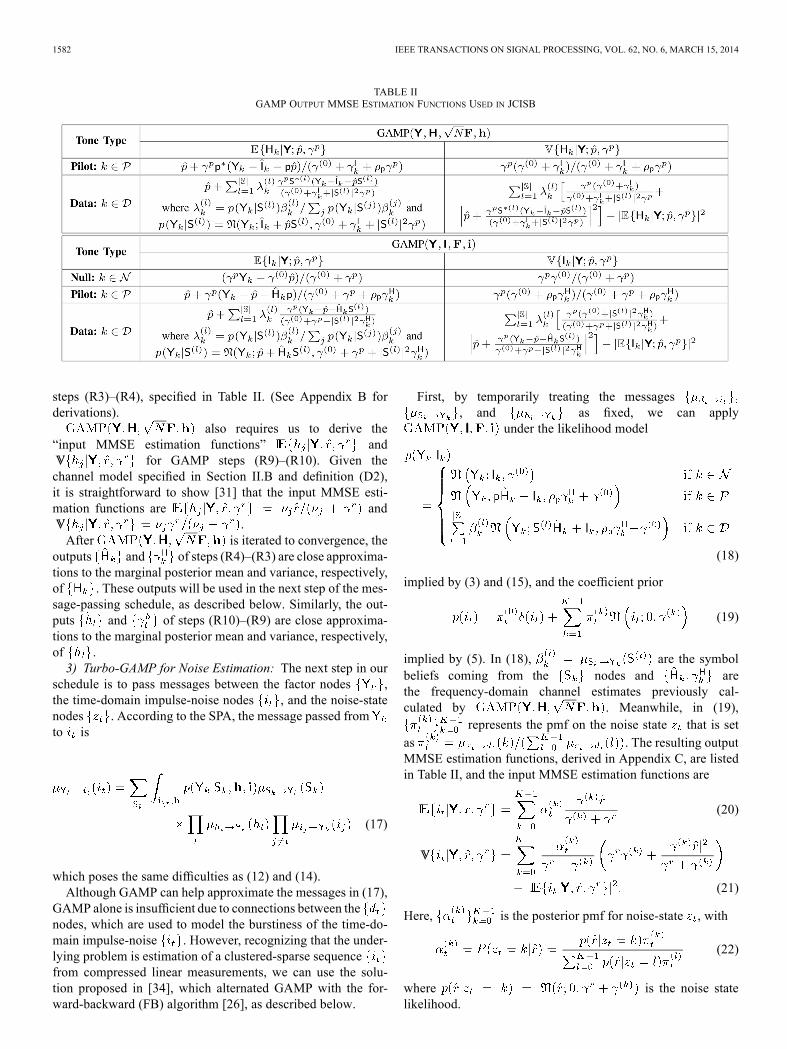
Fig. 6. Uncoded versus for OFDM with 256 total tones and 60null tones under a known trivial channel for (a) i.i.d GM and (b) GHMM noise.Red traces denote 4-QAM while blue traces denote 16-QAM.
Fig. 6(b) then shows under GHMM (i.e., bursty) noise.Comparing Fig. 6(b) to (a), we see that the burstiness of thenoise causes the of all receivers to degrade significantly.Moreover, this degradation persists when the JIS receiver usesMC iterations, even though the results in Fig. 5 showonly about a 1 dB loss due to burstiness. We attribute thesensitivity to the fact that the noise burstiness makes someOFDM-symbols much more noise-corrupted than others, andthose heavily corrupted symbols lead to a degradation in ,reported in Fig. 6(b), that exceeds the degradation expectedof 1 dB i.i.d. Gaussian noise (unreported simulations showthat the errors in GHMM noise estimation under JIS-FB arenon-Gaussian and dependent). Regardless, Fig. 6(b) showsthat the FB-assisted JIS receiver significantly outperformsnon-FB-assisted JIS, GI, and the state-of-the-art SBL algo-rithm, especially at medium . To investigate whether thekink in the JIS FB trace was due to suboptimality of the FBnoise-state inference, we simulated a genie-aided receiver thatknows the true state of the GHMM noise at each time index.Since the genie trace also exhibits the kink, it is evidently notdue to suboptimality of FB.
D. Impact of Pilot and Null Tone Placement
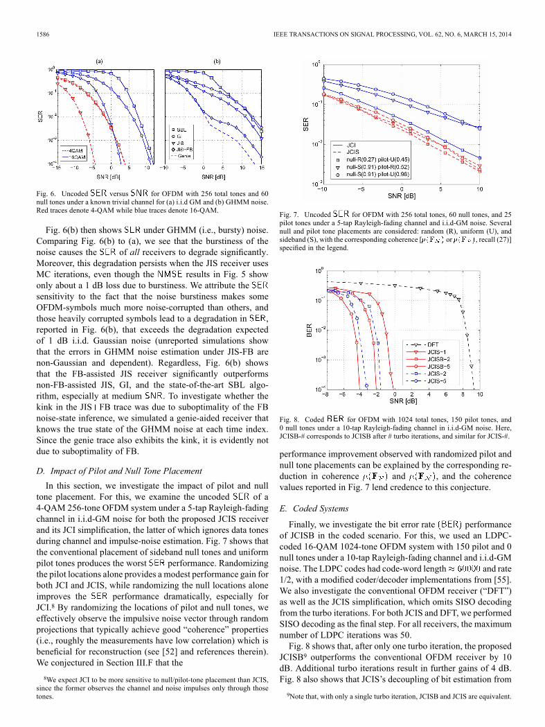
In this section, we investigate the impact of pilot and nulltone placement. For this, we examine the uncoded of a4-QAM 256-tone OFDM system under a 5-tap Rayleigh-fadingchannel in i.i.d-GM noise for both the proposed JCIS receiverand its JCI simplification, the latter of which ignores data tonesduring channel and impulse-noise estimation. Fig. 7 shows thatthe conventional placement of sideband null tones and uniformpilot tones produces the worst performance. Randomizingthe pilot locations alone provides a modest performance gain forboth JCI and JCIS, while randomizing the null locations aloneimproves the performance dramatically, especially forJCI.8 By randomizing the locations of pilot and null tones, weeffectively observe the impulsive noise vector through randomprojections that typically achieve good “coherence” properties(i.e., roughly the measurements have low correlation) which isbeneficial for reconstruction (see [52] and references therein).We conjectured in Section III.F that the
8We expect JCI to be more sensitive to null/pilot-tone placement than JCIS,since the former observes the channel and noise impulses only through thosetones.
Fig. 7. Uncoded for OFDM with 256 total tones, 60 null tones, and 25pilot tones under a 5-tap Rayleigh-fading channel and i.i.d-GM noise. Severalnull and pilot tone placements are considered: random (R), uniform (U), andsideband (S), with the corresponding coherence [ or , recall (27)]specified in the legend.
Fig. 8. Coded for OFDM with 1024 total tones, 150 pilot tones, and0 null tones under a 10-tap Rayleigh-fading channel in i.i.d-GM noise. Here,JCISB-# corresponds to JCISB after # turbo iterations, and similar for JCIS-#.
performance improvement observed with randomized pilot andnull tone placements can be explained by the corresponding re-duction in coherence and , and the coherencevalues reported in Fig. 7 lend credence to this conjecture.
E. Coded Systems
Finally, we investigate the bit error rate performanceof JCISB in the coded scenario. For this, we used an LDPC-coded 16-QAM 1024-tone OFDM system with 150 pilot and 0null tones under a 10-tap Rayleigh-fading channel and i.i.d-GMnoise. The LDPC codes had code-word length and rate1/2, with a modified coder/decoder implementations from [55].We also investigate the conventional OFDM receiver (“DFT”)as well as the JCIS simplification, which omits SISO decodingfrom the turbo iterations. For both JCIS and DFT, we performedSISO decoding as the final step. For all receivers, the maximumnumber of LDPC iterations was 50.Fig. 8 shows that, after only one turbo iteration, the proposed
JCISB9 outperforms the conventional OFDM receiver by 10dB. Additional turbo iterations result in further gains of 4 dB.Fig. 8 also shows that JCIS’s decoupling of bit estimation from
9Note that, with only a single turbo iteration, JCISB and JCIS are equivalent.
NASSAR et al.: JOINT OFDM CHANNEL ESTIMATION 1587
channel, impulse, and symbol estimation costs approximately1 dB.
V. CONCLUSION
In a this paper, we presented a factor-graph approach toOFDM reception in multipath distorted and impulse-noisecorrupted channels that performs near-optimal joint channel,impulse-noise, symbol, and bit (JCISB) estimation. Ourapproach merges recent work on generalized approximate mes-sage passing (GAMP) [31], its “turbo” extension to larger factorgraphs [34], and soft-input-soft-output SISO decoding [35].Extensive numerical simulations show that the proposed JCISBreceiver provides drastic performance gains over existing re-ceivers for OFDM in impulsive noise, and performs within 1dBof the matched-filter bound, all while matching the complexityorder of the conventional OFDM receiver. Furthermore, JCISBis easily parallelized, providing a natural mapping to FPGAimplementations (see [36] for a recent FPGA implementationof the GI receiver). Additional numerical simulations inves-tigated the impact of JCISB simplifications, noise modelingand mitigation, and null/pilot tone placement. Throughoutthis paper we have assumed prior knowledge of the noiseparameters while in practical settings this information mighthave to be estimated by the receiver. Incorporating parameterestimation in the proposed framework is an interesting topicfor future work.
The GAMP algorithm, an extension of AMP from [46],was developed in [31] to address the estimation of a vectorof independent possibly-non-Gaussian random variablesthat are linearly mixed via a linear transform toform and subsequently observed as
according to the general likelihood function. The GAMP algorithm is intended
for the case when the dimensions and are both large, inwhich case the central limit theorem suggests approximatingthe product of messages flowing leftward into each factor node
in Fig. 9 as andthe product of messages flowing rightward into each variablenode as , where the quanti-ties , and can be computed from Table I. Similarly,to remain computationally tractable, the pdf representing eachmessage leaving a factor or a variable node is simplified bytaking its second order Taylor series expansion. As a result,each of those messages can be approximated by two parame-ters resulting from the Taylor expansion. The corresponding“ ” algorithm is summarized in Table I. Thedetailed derivation and theoretical guarantees of the GAMPalgorithm are beyond the scope of this paper; we refer theinterested reader to [31] and [48] for more information.
APPENDIX BDERIVATION OF LIKELIHOOD
This Appendix derives the output MMSE estimation func-tions and VV used in steps
Fig. 9. Factor graph used to derive GAMP with illustrations of messageapproximations.
(R3)–(R4) of . We start with the caseof data tones , where
is Gaussian when conditioned on , and so according tothe definition (D1) in Table I this is a standard linear MMSEproblem whose solution is given by ([56], Ch. 12),
(29)
Given the belief about symbol and the decouplingachieved by GAMP between and ( depends only on), the law of total expectation implies
(30)
(31)
where
(32)
is the posterior symbol probability and. Similarly, the law of
total variance implies
VV
VV
VV (33)
(34)
The derivation for pilot tones reduces to the above under, and .
APPENDIX CDERIVATION OF LIKELIHOOD
This Appendix derives the output MMSE estimationfunctions and VV used in steps
1588 IEEE TRANSACTIONS ON SIGNAL PROCESSING, VOL. 62, NO. 6, MARCH 15, 2014
(R9)–(R10) of . We start with the case of datatones , where
is Gaussian when conditioned on , and so according tothe definition (D1) in Table I this is a standard linear MMSEproblem whose solution is given by ([56], Ch. 12),
(35)
Given the belief about symbol and the decouplingachieved by GAMP between and ( depends only on ),the law of total expectation implies
(36)
(37)
where is the posterior symbol probabilityfrom (32) but now with
. Similarly, thelaw of total variance implies
VV
VV
VV
(38)
The derivation for pilot tones reduces to the aboveunder , and . Meanwhile, thederivation for null tones is the special case of pilots with
.
ACKNOWLEDGMENT
The authors would like to express gratitude to Dr. Omar ElAyach for many useful discussions and suggestions.
REFERENCES[1] D. Tse and P. Viswanath, Fundamentals of Wireless Communication.
Cambridge, U.K.: Cambridge Univ. Press, 2005.[2] K. Blackard, T. Rappaport, and C. Bostian, “Measurements and models
of radio frequency impulsive noise for indoor wireless communica-tions,” IEEE J. Sel. Areas Commun., vol. 11, no. 7, pp. 991–1001, 1993.
[3] W. Lauber and J. Bertrand, “Statistics of motor vehicle ignition noiseat VHF/UHF,” IEEE Trans. Electromagn. Compat., vol. 41, no. 3, pp.257–259, 1999.
[4] M. Sanchez, L. de Haro, M. Ramon, A. Mansilla, C. Ortega, and D.Oliver, “Impulsive noise measurements and characterization in a UHFdigital TV channel,” IEEE Trans. Electromagn. Compat., vol. 41, no.2, pp. 124–136, 1999.
[5] M. Sanchez, A. Alejos, and I. Cuinas, “Urban wide-band measure-ment of the UMTS electromagnetic environment,” IEEE Trans. Veh.Technol., vol. 53, no. 4, pp. 1014–1022, 2004.
[6] M. Nassar, X. Lin, and B. L. Evans, “Stochastic modeling of mi-crowave oven interference in WLANs,” in Proc. IEEE Int. Conf.Commun., 2011, pp. 1–6.
[7] M. Nassar, K. Gulati, M. DeYoung, B. L. Evans, and K. Tinsley,“Mitigating near-field interference in laptop embedded wirelesstransceivers,” J. Signal Process. Syst., vol. 63, pp. 1–12, 2011.
[8] M. Zimmermann and K. Dostert, “Analysis and modeling of impulsivenoise in broad-band powerline communications,” IEEE Trans. Electro-magn. Compat., vol. 44, no. 1, pp. 249–258, 2002.
[9] M. Nassar, K. Gulati, Y. Mortazavi, and B. L. Evans, “Statistical mod-eling of asynchronous impulsive noise in powerline communicationnetworks,” in Proc. IEEE Global Commun. Conf., 2011, pp. 1–6.
[10] M. Nassar, J. Lin, Y. Mortazavi, A. Dabak, I. H. Kim, and B. L. Evans,“Local utility power line communications in the 3–500 KHz band:Channel impairments, noise, and standards,” IEEE Signal Process.Mag., vol. 29, no. 5, pp. 116–127, 2012.
[11] S. Zhidkov, “Analysis and comparison of several simple impul-sive noise mitigation schemes for OFDM receivers,” IEEE Trans.Commun., vol. 56, no. 1, pp. 5–9, 2008.
[12] D.-F. Tseng, Y. Han, W. H. Mow, L.-C. Chang, and A. Vinck, “Robustclipping for OFDM transmissions over memoryless impulsive noisechannels,” IEEE Commun. Lett., vol. 16, no. 7, pp. 1110–1113, 2012.
[13] J. Haring, Error Tolerant Communication Over the CompoundChannel. New York, NY, USA: Springer-Verlag, 2002.
[14] J. Haring and A. Vinck, “Iterative decoding of codes over complexnumbers for impulsive noise channels,” IEEE Trans. Inf. Theory, vol.49, no. 5, pp. 1251–1260, 2003.
[15] A. Mengi and A. Vinck, “Successive impulsive noise suppression inOFDM,” in Proc. IEEE Int. Symp. Power Line Commun. Appl., 2010,pp. 33–37.
[16] M. Nassar and B. L. Evans, “Low complexity EM-based decoding forOFDM systems with impulsive noise,” in Proc. Asilomar Conf. Sig-nals, Syst. Comput., 2011, pp. 1943–1947.
[17] C.-H. Yih, “Iterative interference cancellation for OFDM signalswith blanking nonlinearity in impulsive noise channels,” IEEE SignalProcess. Lett., vol. 19, no. 3, pp. 147–150, 2012.
[18] J. Wolf, “Redundancy, the discrete Fourier transform, and impulsenoise cancellation,” IEEE Trans. Commun., vol. COM-31, no. 3, pp.458–461, 1983.
[19] F. Abdelkefi, P. Duhamel, and F. Alberge, “Impulsive noise cancella-tion in multicarrier transmission,” IEEE Trans. Commun., vol. 53, no.1, pp. 94–106, 2005.
[20] F. Abdelkefi, P. Duhamel, and F. Alberge, “A necessary condition onthe location of pilot tones for maximizing the correction capacity inOFDM systems,” IEEE Trans. Commun., vol. 55, no. 2, pp. 356–366,2007.
[21] G. Caire, T. Al-Naffouri, and A. Narayanan, “Impulse noise cancella-tion in OFDM: An application of compressed sensing,” in Proc. IEEEInt. Symp. Inf. Theory, 2008, pp. 1293–1297.
[22] L. Lampe, “Bursty impulse noise detection by compressed sensing,” inProc. IEEE Int. Symp. Power Line Commun. Appl., 2011, pp. 29–34.
[23] J. Lin,M. Nassar, and B. L. Evans, “Impulsive noise mitigation in pow-erline communications using sparse Bayesian learning,” IEEE J. Sel.Areas Commun., vol. 31, no. 7, pp. 1172–1183, Jul. 2013.
[24] A. Mehboob, L. Zhang, J. Khangosstar, and K. Suwunnapuk, “Jointchannel and impulsive noise estimation for OFDM based power linecommunication systems using compressed sensing,” in Proc. IEEE Int.Symp. Power Line Commun. Appl., 2013, pp. 203–208.
[25] A. P.Worthen andW. Stark, “Unified design of iterative receivers usingfactor graphs,” IEEE Trans. Inf. Theory, vol. 47, no. 2, pp. 843–849,2001.
[26] C. Bishop, Pattern Recognition and Machine Learning. New York,NY, USA: Springer, 2006.
[27] C. Novak, G.Matz, and F. Hlawatsch, “Factor graph based design of anOFDM-IDMA receiver performing joint data detection, channel esti-mation, and channel length selection,” inProc. IEEE Int. Conf. Acoust.,Speech, Signal Process., 2009, pp. 2561–2564.
[28] Y. Liu, L. Brunel, and J. Boutros, “Joint channel estimation and de-coding using Gaussian approximation in a factor graph over multi-path channel,” in Proc. IEEE Int. Symp. Pers., Indoor Mobile RadioCommun., 2009, pp. 3164–3168.
[29] G. Kirkelund, C. Manchon, L. Christensen, E. Riegler, and B. Fleury,“Variational message-passing for joint channel estimation and de-coding in MIMO-OFDM,” in Proc. IEEE Global Telecommun. Conf.,2010, pp. 1–6.
[30] P. Schniter, “A message-passing receiver for BICM-OFDM over un-known clustered-sparse channels,” IEEE J. Sel. Topics Signal Process.,vol. 5, no. 8, pp. 1462–1474, 2011.
[31] S. Rangan, “Generalized approximate message passing for estimationwith random linear mixing,” in Proc. IEEE Int. Symp. Inf. Theory,2011, pp. 2174–2178, (See also longer version in Arxiv:1010.5141).
[32] P. Schniter, “Belief-propagation-based joint channel estimation and de-coding for spectrally efficient communication over unknown sparsechannels,” Phys. Commun., vol. 5, no. 3, pp. 91–101, 2012.
[33] A. P. Kannu and P. Schniter, “On communication over unknown sparsefrequency-selective block-fading channels,” IEEE Trans. Inf. Theory,vol. 56, no. 6, pp. 6619–6632, Oct. 2011.
NASSAR et al.: JOINT OFDM CHANNEL ESTIMATION 1589
[34] P. Schniter, “Turbo reconstruction of structured sparse signals,” inProc. Conf. Inf. Sci. Syst., 2010, pp. 1–6.
[35] D. MacKay, Information Theory, Inference, and Learning Algo-rithms. Cambridge, MA, USA: Cambridge Univ. Press, 2003.
[36] K. F. Nieman, M. Nassar, J. Lin, and B. L. Evans, “FPGA implemen-tation of a message-passing OFDM receiver for impulsive noise chan-nels,” presented at the Asilomar Conf. Signals, Syst., Comput., PacificGrove, CA, USA, Nov. 3–6, 2013.
[37] P. Schniter and D. Meng, “A message-passing receiver forBICM-OFDM over unknown time-varying sparse channels,” pre-sented at the Allerton Conf. Commun., Control, Comput., Monticello,IL, USA, Sep. 2011, Invited Paper.
[38] D. Middleton, “Non-Gaussian noise models in signal processing fortelecommunications: New methods an results for class A and class Bnoise models,” IEEE Trans. Inf. Theory, vol. 45, no. 4, pp. 1129–1149,1999.
[39] J. Ilow and D. Hatzinakos, “Analytic alpha-stable noise modeling in aPoisson field of interferers or scatterers,” IEEE Trans. Signal Process.,vol. 46, no. 6, pp. 1601–1611, 1998.
[40] K. Gulati, B. L. Evans, J. Andrews, and K. Tinsley, “Statistics ofco-channel interference in a field of Poisson and Poisson-Poissonclustered interferers,” IEEE Trans. Signal Process., vol. 58, no. 12,pp. 6207–6222, 2010.
[41] S. Fruhwirth-Schnatter, Finite Mixture and Markov SwitchingModels. New York, NY, USA: Springer, 2006.
[42] G. F. Cooper, “The computational complexity of probabilistic in-ference using Bayesian belief networks,” Artif. Intell., vol. 42, pp.393–405, 1990.
[43] J. Boutros and G. Caire, “Iterative multiuser joint decoding: Unifiedframework and asymptotic analysis,” IEEE Trans. Inf. Theory, vol. 48,no. 7, pp. 1772–1793, 2002.
[44] D. Guo and C.-C. Wang, “Random sparse linear systems observed viaarbitrary channels: A decoupling principle,” in Proc. IEEE Int. Symp.Inf. Theory, 2007, pp. 946–950.
[45] R. McEliece, D. MacKay, and J.-F. Cheng, “Turbo decoding as aninstance of Pearl’s belief propagation algorithm,” IEEE J. Sel. AreasCommun., vol. 16, no. 2, pp. 140–152, 1998.
[46] D. Donoho, A. Maleki, and A. Montanari, “Message passing algo-rithms for compressed sensing,” in Proc. Natl. Acad. Sci., 2009, vol.106, pp. 18 914–18 919.
[47] M. Bayati and A. Montanari, “The dynamics of message passing ondense graphs, with applications to compressed sensing,” IEEE Trans.Inf. Theory, vol. 57, no. 2, pp. 764–785, 2011.
[48] A. Javanmard and A. Montanari, “State evolution for general approx-imate message passing algorithms, with applications to spatial cou-pling,” Nov. 2012, arXiv:1211.5164.
[49] H. Monajemi, S. Jafarpour, andM. Gavish, “Stat 330/CME 362 collab-oration, and D. L. Donoho Deterministic matrices matching the com-pressed sensing phase transitions of Gaussian random matrices,” inProc. Natl. Acad. Sci., Jan. 2013, vol. 110, no. 4, pp. 1181–1186.
[50] R. Negi and J. Cioffi, “Pilot tone selection for channel estimation ina mobile OFDM system,” IEEE Trans. Consum. Eletron., vol. 44, pp.1122–1128, Aug. 1998.
[51] Powerline Related Intelligent Metering Evolution (PRIME), Prime Al-liance Std. [Online]. Available: http://www.prime-alliance.org
[52] C. Studer, P. Kuppinger, G. Pope, and H. Bolcskei, “Recovery ofsparsely corrupted signals,” IEEE Trans. Inf. Theory, vol. 58, no. 5,pp. 3115–3130, 2012.
[53] A. Spaulding and D. Middleton, “Optimum reception in an impul-sive interference environment-part I: Coherent detection,” IEEE Trans.Commun., vol. COM-25, no. 9, pp. 910–923, 1977.
[54] J. P. Vila and P. Schniter, “Expectation-maximization gaussian-mix-ture approximate message passing,” IEEE Trans. Signal Process., vol.61, no. 19, pp. 4658–4672, Oct. 2013.
[55] I. Kozintsev, Matlab Programs for Encoding and Decoding of LDPCCodes Over GF(2M) [Online]. Available: http://www.kozintsev.net/soft.html
[56] S. M. Kay, Fundamentals of Statistical Signal Processing: EstimationTheory. Englewood Cliffs, NJ, USA: Prentice-Hall, 1993.
Marcel Nassar (M’05) received the B.E. degree incomputer and communications engineering, with aminor degree in mathematics, from the AmericanUniversity of Beirut in 2006, and the M.S. and Ph.D.degrees in electrical and computer engineering fromThe University of Texas at Austin in 2008 and 2013,respectively.During his studies, he interned at the University of
California, Berkeley in 2005, at Intel Corporation in2008 and 2009, and at Texas Instruments in 2011 and2012. After receiving his Ph.D. degree, he joined the
Mobile Solutions Lab at Samsung Research America, CA as a Senior ResearchEngineer. His interests lie at the intersection of signal processing and machinelearning with applications to statistical modeling and mitigation of interferencein communication systems.Dr. Nassar received the Best Paper Award at the 2013 IEEE International
Symposium on Power Line Communications and Its Applications, and secondplace in the Student Paper Contest at the 2013 Asilomar Conference on Signals,Systems, and Computers.
Philip Schniter (F’14) received the B.S. and M.S.degrees in electrical engineering from the Universityof Illinois at Urbana-Champaign in 1992 and 1993,respectively, and the Ph.D. degree in electrical engi-neering from Cornell University, Ithaca, NY, in 2000.From 1993 to 1996, he was with Tektronix Inc.,
Beaverton, OR, as a systems engineer. After re-ceiving the Ph.D. degree, he joined the Departmentof Electrical and Computer Engineering at The OhioState University, Columbus, where he is currentlya Professor and a member of the Information Pro-
cessing Systems (IPS) Lab. In 2008–2009, he was a Visiting Professor atEurecom, Sophia Antipolis, France, and Supélec, Gif-sur-Yvette, France. Hisareas of interest currently include signal processing, machine learning, andwireless communications and networks.Dr. Schniter received the National Science Foundation CAREER Award in
2003, he was elected to serve on the IEEE SPCOM Technical Committee from2005 to 2010 and on the IEEE SAM Technical Committee since 2013.
Brian L. Evans (F’09) received the B.S.E.E.C.S(1987) degree from the Rose-Hulman Institute ofTechnology, and the MSEE (1988) and Ph.D. E.E.(1993) degrees from the Georgia Institute of Tech-nology. From 1993 to 1996, he was a PostdoctoralResearcher at the University of California, Berkeley.In 1996, he joined the faculty at UT Austin.He holds the Engineering Foundation Professor-
ship at UT Austin. His research bridges the gap be-tween digital signal processing theory and embeddedreal-time implementation. His research interests in-
clude wireless interference mitigation, smart grid communications, smart phonevideo acquisition, and cloud radio access networks. Prof. Evans has publishedmore than 220 refereed conference and journal papers, and graduated 21 Ph.D.and 9 M.S. students.Dr. Evans received the Best Paper Award at the 2013 IEEE International Sym-
posium on Power Line Communications and Its Applications, and a Top 10%Paper Award at the 2012 IEEE Multimedia Signal Processing Workshop. Hehas also received three teaching awards at UT Austin: Gordon Lepley Memo-rial ECE Teaching Award (2008), Texas Exes Teaching Award (2011) and HKNOutstanding ECE Professor (2012). He received a 1997 US National ScienceFoundation CAREER Award.