MIT OpenCourseWare http://ocw.mit.edu 16.323 Principles of Optimal Control Spring 2008 For information about citing these materials or our Terms of Use, visit: http://ocw.mit.edu/terms.

16.323 Lecture 4

HJB Equation

DP in continuous time •

• HJB Equation

• Continuous LQR

Factoids: for symmetric R

∂uT Ru= 2u T R

∂u

∂Ru = R

∂u

�

�

Spr 2008 16.323 4–1 DP in Continuous Time

• Have analyzed a couple of approximate solutions to the classic control problem of minimizing:

tf

min J = h(x(tf ), tf ) + g(x(t), u(t), t) dt t0

subject to

x = a(x, u, t)

x(t0) = given

m(x(tf ), tf ) = 0 set of terminal conditions

u(t) ∈ U set of possible constraints

• Previous approaches discretized in time, state, and control actions

– Useful for implementation on a computer, but now want to consider the exact solution in continuous time

– Result will be a nonlinear partial differential equation called the Hamilton-Jacobi-Bellman equation (HJB) – a key result.

• First step: consider cost over the interval [t, tf ], where t ≤ tf of any control sequence u(τ ), t ≤ τ ≤ tf

tf

J(x(t), t, u(τ )) = h(x(tf ), tf ) + g(x(τ ), u(τ ), τ ) dτ t

– Clearly the goal is to pick u(τ ), t ≤ τ ≤ tf to minimize this cost.

J�(x(t), t) = min J(x(t), t, u(τ )) u(τ)∈Ut≤τ≤tf

June 18, 2008

� � �

� � � �

Spr 2008 16.323 4–2

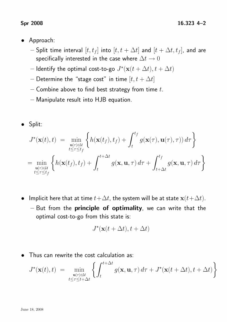
• Approach:

– Split time interval [t, tf ] into [t, t + Δt] and [t + Δt, tf ], and are specifically interested in the case where Δt 0→

– Identify the optimal cost-to-go J�(x(t + Δt), t + Δt)

– Determine the “stage cost” in time [t, t + Δt]

– Combine above to find best strategy from time t.

– Manipulate result into HJB equation.

• Split: tf

J�(x(t), t) = min h(x(tf ), tf ) + g(x(τ ), u(τ ), τ )) dτ tu(τ)∈U

t≤τ≤tf

t+Δt tf

= min h(x(tf ), tf ) + g(x, u, τ ) dτ + g(x, u, τ ) dτ t t+Δtu(τ)∈U

t≤τ ≤tf

• Implicit here that at time t+Δt, the system will be at state x(t+Δt).

– But from the principle of optimality, we can write that the optimal cost-to-go from this state is:

J�(x(t + Δt), t + Δt)

Thus can rewrite the cost calculation as: • �� t+Δt �

J�(x(t), t) = min g(x, u, τ ) dτ + J�(x(t + Δt), t + Δt) tu(τ )∈U

t≤τ≤t+Δt

June 18, 2008

� �

� �

Spr 2008 16.323 4–3

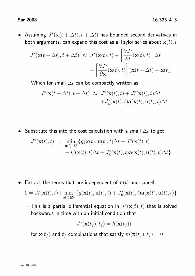
• Assuming J�(x(t + Δt), t + Δt) has bounded second derivatives in both arguments, can expand this cost as a Taylor series about x(t), t

∂J�

J�(x(t + Δt), t + Δt) ≈ J�(x(t), t) + (x(t), t) Δt ∂t

∂J�

+ (x(t), t) (x(t + Δt) − x(t))∂x

– Which for small Δt can be compactly written as:

J�(x(t + Δt), t + Δt) ≈ J�(x(t), t) + J�(x(t), t)Δtt

+Jx�(x(t), t)a(x(t), u(t), t)Δt

• Substitute this into the cost calculation with a small Δt to get

J�(x(t), t) = u(t)∈U

{g(x(t), u(t), t)Δt + J�(x(t), t)min

+J�(x(t), t)Δt + J�(x(t), t)a(x(t), u(t), t)Δt}t x

• Extract the terms that are independent of u(t) and cancel

0 = J�(x(t), t)+ min (x(t), t)a(x(t), u(t), t)}u(t)∈U

{g(x(t), u(t), t) + J� t x

– This is a partial differential equation in J�(x(t), t) that is solved backwards in time with an initial condition that

J�(x(tf ), tf ) = h(x(tf ))

for x(tf ) and tf combinations that satisfy m(x(tf ), tf ) = 0

June 18, 2008

Spr 2008 16.323 4–4 HJB Equation

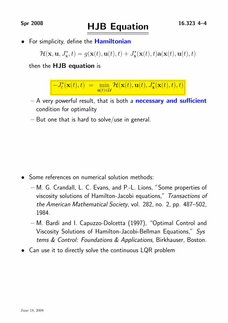
For simplicity, define the Hamiltonian •

H(x, u, Jx�, t) = g(x(t), u(t), t) + Jx

�(x(t), t)a(x(t), u(t), t)

then the HJB equation is

−J� t (x(t), t) = min

u(t)∈U H(x(t), u(t), J�

x(x(t), t), t)

– A very powerful result, that is both a necessary and sufficient condition for optimality

– But one that is hard to solve/use in general.

Some references on numerical solution methods: •

– M. G. Crandall, L. C. Evans, and P.-L. Lions, ”Some properties of viscosity solutions of Hamilton-Jacobi equations,” Transactions of the American Mathematical Society, vol. 282, no. 2, pp. 487–502, 1984.

– M. Bardi and I. Capuzzo-Dolcetta (1997), “Optimal Control and Viscosity Solutions of Hamilton-Jacobi-Bellman Equations,” Sys­

tems & Control: Foundations & Applications, Birkhauser, Boston.

Can use it to directly solve the continuous LQR problem •

June 18, 2008

�

Spr 2008 16.323 4–5 HJB Simple Example

• Consider the system with dynamics

x = Ax + u

for which A + AT = 0 and �u� ≤ 1, and the cost functiontf

J = dt = tf0

Then the Hamiltonian is •

H = 1 + J�(Ax + u)x

and the constrained minimization of H with respect to u gives

u � = −(Jx�)T/�Jx

��

• Thus the HJB equation is:

−Jt� = 1 + Jx�(Ax) − �Jx

��

• As a candidate solution, take J�(x) = xT x/�x� = �x�, which is not an explicit function of t, so

T

Jx � =

xand Jt

� = 0 �x�

which gives: T

0 = 1 +x

(Ax) − �x� �x� �x�

1 = (x TAx) �x�1 1

= x T (A + AT )x = 0 �x� 2

so that the HJB is satisfied and the optimal control is:

� x u = −

�x�

June 18, 2008

�

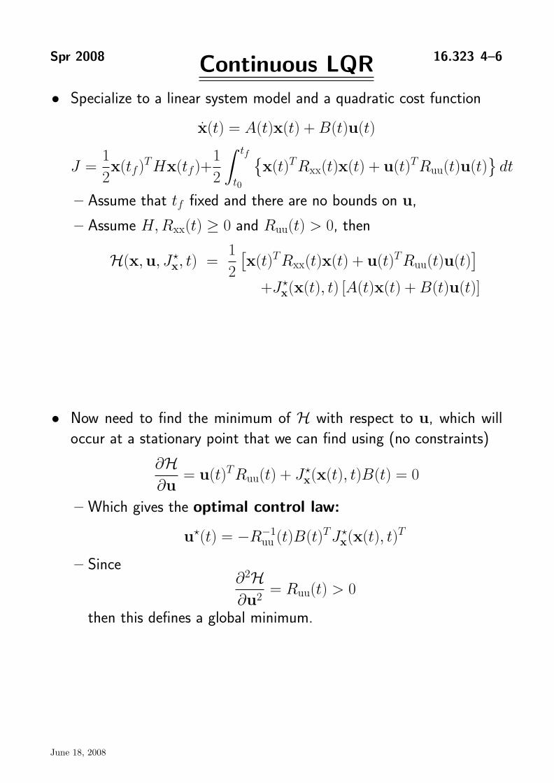
Spr 2008 16.323 4–6 Continuous LQR• Specialize to a linear system model and a quadratic cost function

x(t) = A(t)x(t) + B(t)u(t)

J =1 x(tf )

THx(tf )+1 tf �

x(t)TRxx(t)x(t) + u(t)TRuu(t)u(t) � dt

2 2 t0

– Assume that tf fixed and there are no bounds on u,

– Assume H,Rxx(t) ≥ 0 and Ruu(t) > 0, then

1 � � H(x, u, Jx

�, t) = x(t)TRxx(t)x(t) + u(t)TRuu(t)u(t)2

+Jx�(x(t), t) [A(t)x(t) + B(t)u(t)]

• Now need to find the minimum of H with respect to u, which will occur at a stationary point that we can find using (no constraints)

∂H = u(t)TRuu(t) + J�(x(t), t)B(t) = 0

∂u x

– Which gives the optimal control law:

u �(t) = −R−1(t)B(t)TJ�(x(t), t)T uu x

– Since ∂2H

= Ruu(t) > 0 ∂u2

then this defines a global minimum.

June 18, 2008

� �

Spr 2008 16.323 4–7

• Given this control law, can rewrite the Hamiltonian as:

H(x, u �, J�, t) =x

1 � � 2

x(t)TRxx(t)x(t) + J�(x(t), t)B(t)R−1(t)Ruu(t)R−1(t)B(t)TJx uu uu

�(x(t), t)T x

+J�(x(t), t) A(t)x(t) − B(t)R−1(t)B(t)TJ�(x(t), t)Tx uu x

1= x(t)TRxx(t)x(t) + Jx

�(x(t), t)A(t)x(t)2

1−2 Jx�(x(t), t)B(t)Ru

−u 1(t)B(t)TJx

�(x(t), t)T

• Might be difficult to see where this is heading, but note that the boundary condition for this PDE is:

J�(x(tf ), tf ) = 1 x T (tf )Hx(tf )

2– So a candidate solution to investigate is to maintain a quadratic

form for this cost for all time t. So could assume that 1

J�(x(t), t) = x T (t)P (t)x(t), P (t) = PT (t)2

and see what conditions we must impose on P (t). 6

– Note that in this case, J� is a function of the variables x and t7

∂J�

= x T (t)P (t)∂x

∂J� 1= x T (t)P (t)x(t)

∂t 2• To use HJB equation need to evaluate:

−J�(x(t), t) = min , t)u(t)∈U

H(x(t), u(t), J� t x

6See AM, pg. 21 on how to avoid having to make this assumption.

7Partial derivatives taken wrt one variable assuming the other is fixed. Note that there are 2 independent variables in this problem x and t. x is time-varying, but it is not a function of t.

June 18, 2008

Spr 2008 16.323 4–8

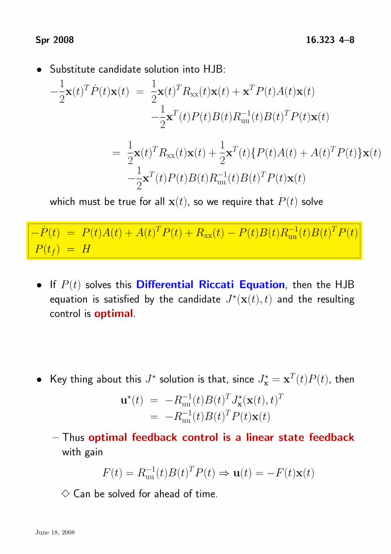
Substitute candidate solution into HJB: • 1 1 −2 x(t)T P (t)x(t) =

2 x(t)TRxx(t)x(t) + x TP (t)A(t)x(t)

1 −2 x T (t)P (t)B(t)R−1(t)B(t)TP (t)x(t)uu

=1 x(t)TRxx(t)x(t) +

1 x T (t){P (t)A(t) + A(t)TP (t)}x(t)

2 2 1 −2 x T (t)P (t)B(t)R−1(t)B(t)TP (t)x(t)uu

which must be true for all x(t), so we require that P (t) solve

−P (t) = P (t)A(t) + A(t)T P (t) + Rxx(t) − P (t)B(t)R−1 uu (t)B(t)T P (t)

P (tf ) = H

• If P (t) solves this Differential Riccati Equation, then the HJB equation is satisfied by the candidate J�(x(t), t) and the resulting control is optimal.

• Key thing about this J� solution is that, since Jx � = xT (t)P (t), then

u �(t) = −R−1(t)B(t)TJ�(x(t), t)T uu x

= −R−1(t)B(t)TP (t)x(t)uu

– Thus optimal feedback control is a linear state feedback with gain

F (t) = R−1(t)B(t)TP (t) ⇒ u(t) = −F (t)x(t)uu

�Can be solved for ahead of time.

June 18, 2008

Spr 2008 16.323 4–9

• As before, can evaluate the performance of some arbitrary time-

varying feedback gain u = −G(t)x(t), and the result is that

1JG = x TS(t)x

2where S(t) solves

−S(t) = {A(t) − B(t)G(t)}TS(t) + S(t){A(t) − B(t)G(t)}

+ Rxx(t) + G(t)TRuu(t)G(t)

S(tf ) = H

– Since this must be true for arbitrary G, then would expect that this reduces to Riccati Equation if G(t) ≡ R−1(t)BT (t)S(t)uu

• If we assume LTI dynamics and let tf → ∞, then at any finite time t, would expect the Differential Riccati Equation to settle down to a steady state value (if it exists) which is the solution of

PA + ATP + Rxx − PBR−1BTP = 0 uu

– Called the (Control) Algebraic Riccati Equation (CARE)

– Typically assume that Rxx = CzTRzzCz, Rzz > 0 associated with

performance output variable z(t) = Czx(t)

June 18, 2008

Spr 2008 16.323 4–10 LQR Observations • With terminal penalty, H = 0, the solution to the differential Riccati

Equation (DRE) approaches a constant iff the system has no poles that are unstable, uncontrollable8, and observable9 by z(t)

– If a constant steady state solution to the DRE exists, then it is a positive semi-definite, symmetric solution of the CARE.

• If [A,B,Cz] is both stabilizable and detectable (i.e. all modes are stable or seen in the cost function), then:

– Independent of H ≥ 0, the steady state solution Pss of the DRE approaches the unique PSD symmetric solution of the CARE.

• If a steady state solution exists Pss to the DRE, then the closed-loop system using the static form of the feedback

u(t) = −R−1BTPssx(t) = −Fssx(t)uu

is asymptotically stable if and only if the system [A,B,Cz] is stabilizable and detectable.

– This steady state control minimizes the infinite horizon cost func­

tion lim J for all H ≥ 0 tf →∞

• The solution Pss is positive definite if and only if the system [A,B,Cz] is stabilizable and completely observable.

• See Kwakernaak and Sivan, page 237, Section 3.4.3.

816.31 Notes on Controllability

916.31 Notes on Observability

June 18, 2008

�

�

� � �

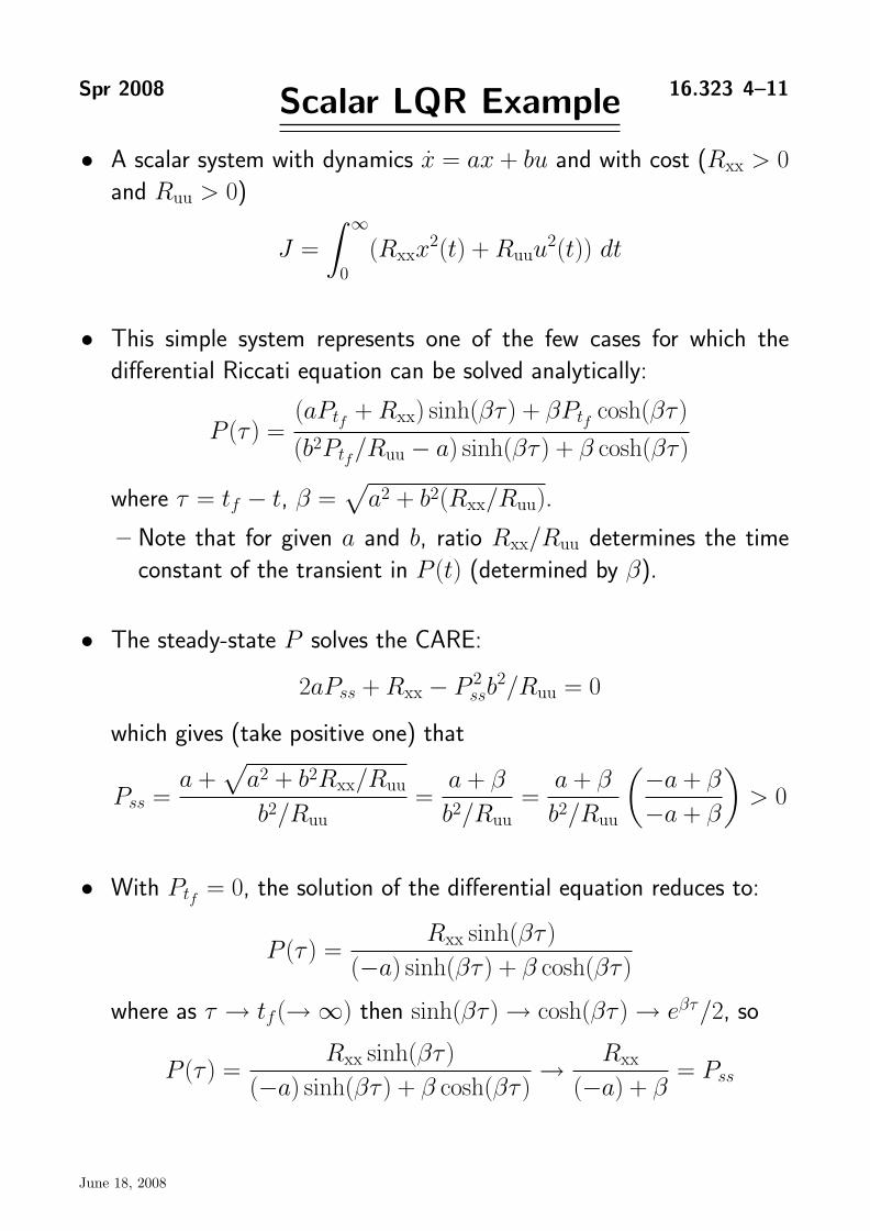
Spr 2008 16.323 4–11 Scalar LQR Example

• A scalar system with dynamics x = ax + bu and with cost (Rxx > 0 and Ruu > 0)

J = ∞

(Rxxx 2(t) + Ruuu 2(t)) dt 0

• This simple system represents one of the few cases for which the differential Riccati equation can be solved analytically:

(aPtf + Rxx) sinh(βτ ) + βPtf cosh(βτ ) P (τ ) =

(b2Ptf /Ruu − a) sinh(βτ ) + β cosh(βτ )

where τ = tf − t, β = a2 + b2(Rxx/Ruu).

– Note that for given a and b, ratio Rxx/Ruu determines the time constant of the transient in P (t) (determined by β).

• The steady-state P solves the CARE:

2aPss + Rxx − P 2 b2/Ruu = 0 ss

which gives (take positive one) that

a + a2 + b2Rxx/Ruu a + β a + β −a + β Pss = = = > 0

b2/Ruu b2/Ruu b2/Ruu −a + β

• With Ptf = 0, the solution of the differential equation reduces to:

Rxx sinh(βτ )P (τ ) =

(−a) sinh(βτ ) + β cosh(βτ )

where as τ → tf (→∞) then sinh(βτ ) → cosh(βτ ) → eβτ /2, so

Rxx sinh(βτ ) RxxP (τ ) = = Pss

(−a) sinh(βτ ) + β cosh(βτ ) →

(−a) + β

June 18, 2008

�

� �

�

�

Spr 2008 16.323 4–12

• Then the steady state feedback controller is u(t) = −Kx(t) where

= R−1bPss = a + a2 + b2Rxx/Ruu

Kss uu b

• The closed-loop dynamics are

x = (a − bKss)x = Aclx(t) b �

= a − (a + a2 + b2Rxx/Ruu) x b

= a2 + b2Rxx/Ruu x−

which are clearly stable.

• As Rxx/Ruu →∞, Acl ≈ −|b| Rxx/Ruu

– Cheap control problem

– Note that smaller Ruu leads to much faster response.

• As Rxx/Ruu → 0, K ≈ (a + |a|)/b – Expensive control problem

– If a < 0 (open-loop stable), K ≈ 0 and Acl = a − bK ≈ a

– If a > 0 (OL unstable), K ≈ 2a/b and Acl = a − bK ≈ −a

• Note that in the expensive control case, the controller tries to do as little as possible, but it must stabilize the unstable open-loop system.

– Observation: optimal definition of “as little as possible” is to put the closed-loop pole at the reflection of the open-loop pole about the imaginary axis.

June 18, 2008

Spr 2008 16.323 4–13 Numerical P Integration

• To numerically integrate solution of P , note that we can use standard Matlab integration tools if we can rewrite the DRE in vector form.

– Define a vec operator so that ⎤⎡

vec(P ) =

⎢⎢⎢⎢⎢⎢⎢⎢⎢⎢⎢⎣

P11

P12... P1n

P22

P23... Pnn

⎥⎥⎥⎥⎥⎥⎥⎥⎥⎥⎥⎦

≡ y

– The unvec(y) operation is the straightforward

– Can now write the DRE as differential equation in the variable y

• Note that with τ = tf − t, then dτ = −dt, – t = tf corresponds to τ = 0, t = 0 corresponds to τ = tf

– Can do the integration forward in time variable τ : 0 tf→

Then define a Matlab function as •

doty = function(y);global A B Rxx Ruu %P=unvec(y); %% assumes that P derivative wrt to tau (so no negative)dot P = (P*A + A^T*P+Rxx-P*B*Ruu^{-1}*B^T*P);%doty = vec(dotP); %return

– Which is integrated from τ = 0 with initial condition H

– Code uses a more crude form of integration

June 18, 2008

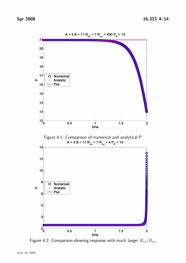
Spr 2008 16.323 4–14

Figure 4.1: Comparison of numerical and analytical P

Figure 4.2: Comparison showing response with much larger Rxx/Ruu

June 18, 2008

Spr 2008 16.323 4–15

Figure 4.3: State response with high and low Ruu. State response with time-varying gain almost indistinguishable – highly dynamic part of x response ends before significant variation in P .

June 18, 2008

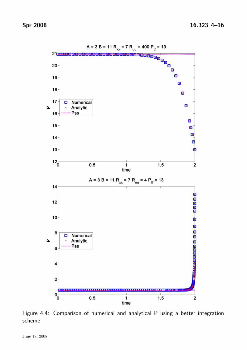
Spr 2008 16.323 4–16

Figure 4.4: Comparison of numerical and analytical P using a better integration scheme

June 18, 2008

1

2

3

4

5

6

7

8

9

10

11

12

13

14

15

16

17

18

19

20

21

22

23

24

25

26

27

28

29

30

31

32

33

34

35

36

37

38

39

40

41

42

43

44

45

46

47

48

49

50

51

52

53

54

55

56

57

58

59

60

61

62

63

64

65

66

67

Spr 2008 16.323 4–17

Numerical Calculation of P

% Simple LQR example showing time varying P and gains % 16.323 Spring 2008 % Jonathan How % reg2.m clear all;close all; set(0, ’DefaultAxesFontSize’, 14, ’DefaultAxesFontWeight’,’demi’) set(0, ’DefaultTextFontSize’, 14, ’DefaultTextFontWeight’,’demi’) global A B Rxx Ruu

A=3;B=11;Rxx=7;Ptf=13;tf=2;dt=.0001;Ruu=20^2;Ruu=2^2;

% integrate the P backwards (crude form)time=[0:dt:tf];P=zeros(1,length(time));K=zeros(1,length(time));Pcurr=Ptf;for kk=0:length(time)-1

P(length(time)-kk)=Pcurr; K(length(time)-kk)=inv(Ruu)*B’*Pcurr; Pdot=-Pcurr*A-A’*Pcurr-Rxx+Pcurr*B*inv(Ruu)*B’*Pcurr; Pcurr=Pcurr-dt*Pdot;

end

options=odeset(’RelTol’,1e-6,’AbsTol’,1e-6)[tau,y]=ode45(@doty,[0 tf],vec(Ptf));Tnum=[];Pnum=[];Fnum=[];for i=1:length(tau)

Tnum(length(tau)-i+1)=tf-tau(i);temp=unvec(y(i,:));Pnum(length(tau)-i+1,:,:)=temp;Fnum(length(tau)-i+1,:)=-inv(Ruu)*B’*temp;

end

% get the SS result from LQR[klqr,Plqr]=lqr(A,B,Rxx,Ruu);

% Analytical predbeta=sqrt(A^2+Rxx/Ruu*B^2);t=tf-time;Pan=((A*Ptf+Rxx)*sinh(beta*t)+beta*Ptf*cosh(beta*t))./...

((B^2*Ptf/Ruu-A)*sinh(beta*t)+beta*cosh(beta*t)); Pan2=((A*Ptf+Rxx)*sinh(beta*(tf-Tnum))+beta*Ptf*cosh(beta*(tf-Tnum)))./...

((B^2*Ptf/Ruu-A)*sinh(beta*(tf-Tnum))+beta*cosh(beta*(tf-Tnum)));

figure(1);clfplot(time,P,’bs’,time,Pan,’r.’,[0 tf],[1 1]*Plqr,’m--’)title([’A = ’,num2str(A),’ B = ’,num2str(B),’ R_{xx} = ’,num2str(Rxx),...

’ R_{uu} = ’,num2str(Ruu),’ P_{tf} = ’,num2str(Ptf)]) legend(’Numerical’,’Analytic’,’Pss’,’Location’,’West’) xlabel(’time’);ylabel(’P’) if Ruu > 10

print -r300 -dpng reg2_1.png;else

print -r300 -dpng reg2_2.png;end

figure(3);clfplot(Tnum,Pnum,’bs’,Tnum,Pan2,’r.’,[0 tf],[1 1]*Plqr,’m--’)title([’A = ’,num2str(A),’ B = ’,num2str(B),’ R_{xx} = ’,num2str(Rxx),...

’ R_{uu} = ’,num2str(Ruu),’ P_{tf} = ’,num2str(Ptf)]) legend(’Numerical’,’Analytic’,’Pss’,’Location’,’West’) xlabel(’time’);ylabel(’P’) if Ruu > 10

print -r300 -dpng reg2_13.png;else

print -r300 -dpng reg2_23.png;end

June 18, 2008

1

2

3

4

5

6

7

8

9

10

11

Spr 2008 16.323 4–18

68

69 Pan2=inline(’((A*Ptf+Rxx)*sinh(beta*t)+beta*Ptf*cosh(beta*t))/((B^2*Ptf/Ruu-A)*sinh(beta*t)+beta*cosh(beta*t))’); 70 x1=zeros(1,length(time));x2=zeros(1,length(time)); 71 xcurr1=[1]’;xcurr2=[1]’; 72 for kk=1:length(time)-1 73 x1(:,kk)=xcurr1; x2(:,kk)=xcurr2; 74 xdot1=(A-B*Ruu^(-1)*B’*Pan2(A,B,Ptf,Ruu,Rxx,beta,tf-(kk-1)*dt))*x1(:,kk); 75 xdot2=(A-B*klqr)*x2(:,kk); 76 xcurr1=xcurr1+xdot1*dt; 77 xcurr2=xcurr2+xdot2*dt; 78 end 79

80 figure(2);clf 81 plot(time,x2,’bs’,time,x1,’r.’);xlabel(’time’);ylabel(’x’) 82 title([’A = ’,num2str(A),’ B = ’,num2str(B),’ R_{xx} = ’,num2str(Rxx),... 83 ’ R_{uu} = ’,num2str(Ruu),’ P_{tf} = ’,num2str(Ptf)]) 84 legend(’K_{ss}’,’K_{analytic}’,’Location’,’NorthEast’) 85 if Ruu > 10 86 print -r300 -dpng reg2_11.png; 87 else 88 print -r300 -dpng reg2_22.png; 89 end

1 function [doy]=doty(t,y); 2 global A B Rxx Ruu; 3 P=unvec(y); 4 dotP=P*A+A’*P+Rxx-P*B*Ruu^(-1)*B’*P; 5 doy=vec(dotP); 6 return

1 function y=vec(P); 2

3 y=[]; 4 for ii=1:length(P); 5 y=[y;P(ii,ii:end)’]; 6 end 7

8 return

function P=unvec(y);

N=max(roots([1 1 -2*length(y)]));P=[];kk=N;kk0=1;for ii=1:N;

P(ii,ii:N)=[y(kk0+[0:kk-1])]’;kk0=kk0+kk;kk=kk-1;

end P=(P+P’)-diag(diag(P)); return

June 18, 2008

� � � �

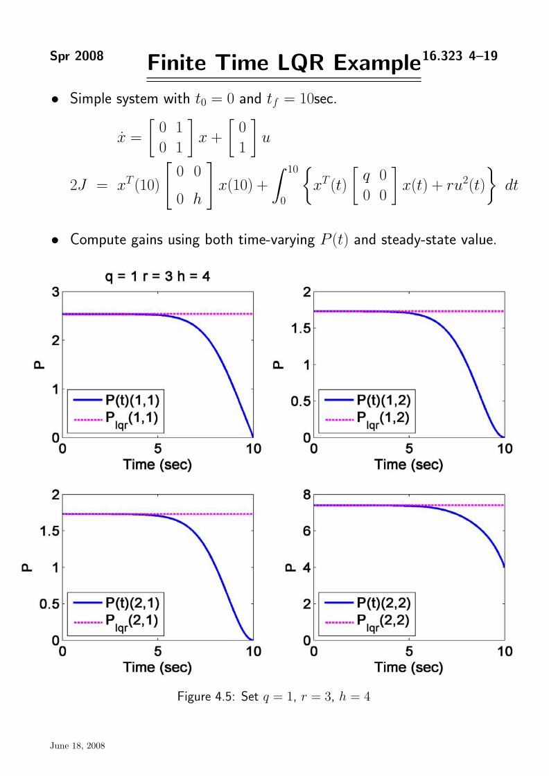
Spr 2008 Finite Time LQR Example16.323 4–19

• Simple system with t0 = 0 and tf = 10sec.

0 1 0 x = x + u

0 1 1 � � � 10 � � � �

2J = xT (10)0 0

x(10) + xT (t) q 0

x(t) + ru 2(t) dt 0 h 0 0 0

• Compute gains using both time-varying P (t) and steady-state value.

Figure 4.5: Set q = 1, r = 3, h = 4

June 18, 2008

Spr 2008 16.323 4–20

• Find state solution x(0) = [1 1]T using both sets of gains

Figure 4.6: Time-varying and constant gains - Klqr = [0.5774 2.4679]

Figure 4.7: State response - Constant gain and time-varying gain almost indistin­guishable because the transient dies out before the time at which the gains start to change – effectively a steady state problem.

• For most applications, the static gains are more than adequate - it is only when the terminal conditions are important in a short-time horizon problem that the time-varying gains should be used.

– Significant savings in implementation complexity & computa­

tion.

June 18, 2008

1

2

3

4

5

6

7

8

9

10

11

12

13

14

15

16

17

18

19

20

21

22

23

24

25

26

27

28

29

30

31

32

33

34

35

36

37

38

39

40

41

42

43

44

45

46

47

48

49

50

51

52

53

54

55

56

57

58

59

60

61

62

63

64

65

66

67

Spr 2008 16.323 4–21

Finite Time LQR Example

% Simple LQR example showing time varying P and gains % 16.323 Spring 2008 % Jonathan How % reg1.m % clear all;%close all; set(0, ’DefaultAxesFontSize’, 14, ’DefaultAxesFontWeight’,’demi’) set(0, ’DefaultTextFontSize’, 14, ’DefaultTextFontWeight’,’demi’) global A B Rxx Ruu jprint = 0;

h=4;q=1;r=3;A=[0 1;0 1];B=[0 1]’;tf=10;dt=.01;Ptf=[0 0;0 h];Rxx=[q 0;0 0];Ruu=r;Ptf=[0 0;0 1];Rxx=[q 0;0 100];Ruu=r;

% alternative calc of Ricc solutionH=[A -B*B’/r ; -Rxx -A’];[V,D]=eig(H); % check order of eigenvaluesPsi11=V(1:2,1:2);Psi21=V(3:4,1:2);Ptest=Psi21*inv(Psi11);

if 0

% integrate the P backwards (crude)time=[0:dt:tf];P=zeros(2,2,length(time));K=zeros(1,2,length(time));Pcurr=Ptf;for kk=0:length(time)-1

P(:,:,length(time)-kk)=Pcurr; K(:,:,length(time)-kk)=inv(Ruu)*B’*Pcurr; Pdot=-Pcurr*A-A’*Pcurr-Rxx+Pcurr*B*inv(Ruu)*B’*Pcurr; Pcurr=Pcurr-dt*Pdot;

end

else% integrate forwards (ODE)options=odeset(’RelTol’,1e-6,’AbsTol’,1e-6)[tau,y]=ode45(@doty,[0 tf],vec(Ptf),options);Tnum=[];Pnum=[];Fnum=[];for i=1:length(tau)

time(length(tau)-i+1)=tf-tau(i); temp=unvec(y(i,:)); P(:,:,length(tau)-i+1)=temp; K(:,:,length(tau)-i+1)=inv(Ruu)*B’*temp;

end

end % if 0

% get the SS result from LQR[klqr,Plqr]=lqr(A,B,Rxx,Ruu);

x1=zeros(2,1,length(time));x2=zeros(2,1,length(time));xcurr1=[1 1]’;xcurr2=[1 1]’;for kk=1:length(time)-1

dt=time(kk+1)-time(kk);x1(:,:,kk)=xcurr1;x2(:,:,kk)=xcurr2;xdot1=(A-B*K(:,:,kk))*x1(:,:,kk);xdot2=(A-B*klqr)*x2(:,:,kk);xcurr1=xcurr1+xdot1*dt;xcurr2=xcurr2+xdot2*dt;

end

June 18, 2008

Spr 2008 16.323 4–22

68 x1(:,:,length(time))=xcurr1;69 x2(:,:,length(time))=xcurr2;70

71 figure(5);clf72 subplot(221)73 plot(time,squeeze(K(1,1,:)),[0 10],[1 1]*klqr(1),’m--’,’LineWidth’,2)74 legend(’K_1(t)’,’K_1’)75 xlabel(’Time (sec)’);ylabel(’Gains’)76 title([’q = ’,num2str(1),’ r = ’,num2str(r),’ h = ’,num2str(h)])77 subplot(222)78 plot(time,squeeze(K(1,2,:)),[0 10],[1 1]*klqr(2),’m--’,’LineWidth’,2)79 legend(’K_2(t)’,’K_2’)80 xlabel(’Time (sec)’);ylabel(’Gains’)81 subplot(223)82 plot(time,squeeze(x1(1,1,:)),time,squeeze(x1(2,1,:)),’m--’,’LineWidth’,2),83 legend(’x_1’,’x_2’)84 xlabel(’Time (sec)’);ylabel(’States’);title(’Dynamic Gains’)85 subplot(224)86 plot(time,squeeze(x2(1,1,:)),time,squeeze(x2(2,1,:)),’m--’,’LineWidth’,2),87 legend(’x_1’,’x_2’)88 xlabel(’Time (sec)’);ylabel(’States’);title(’Static Gains’)89

90 figure(6);clf91 subplot(221)92 plot(time,squeeze(P(1,1,:)),[0 10],[1 1]*Plqr(1,1),’m--’,’LineWidth’,2)93 legend(’P(t)(1,1)’,’P_{lqr}(1,1)’,’Location’,’SouthWest’)94 xlabel(’Time (sec)’);ylabel(’P’)95 title([’q = ’,num2str(1),’ r = ’,num2str(r),’ h = ’,num2str(h)])96 subplot(222)97 plot(time,squeeze(P(1,2,:)),[0 10],[1 1]*Plqr(1,2),’m--’,’LineWidth’,2)98 legend(’P(t)(1,2)’,’P_{lqr}(1,2)’,’Location’,’SouthWest’)99 xlabel(’Time (sec)’);ylabel(’P’)

100 subplot(223) 101 plot(time,squeeze(P(2,1,:)),[0 10],[1 1]*squeeze(Plqr(2,1)),’m--’,’LineWidth’,2), 102 legend(’P(t)(2,1)’,’P_{lqr}(2,1)’,’Location’,’SouthWest’) 103 xlabel(’Time (sec)’);ylabel(’P’) 104 subplot(224) 105 plot(time,squeeze(P(2,2,:)),[0 10],[1 1]*squeeze(Plqr(2,2)),’m--’,’LineWidth’,2), 106 legend(’P(t)(2,2)’,’P_{lqr}(2,2)’,’Location’,’SouthWest’) 107 xlabel(’Time (sec)’);ylabel(’P’) 108 axis([0 10 0 8]) 109 if jprint; print -dpng -r300 reg1_6.png 110 end 111

112 figure(1);clf 113 plot(time,squeeze(K(1,1,:)),[0 10],[1 1]*klqr(1),’r--’,’LineWidth’,3) 114 legend(’K_1(t)(1,1)’,’K_1(1,1)’,’Location’,’SouthWest’) 115 xlabel(’Time (sec)’);ylabel(’Gains’) 116 title([’q = ’,num2str(1),’ r = ’,num2str(r),’ h = ’,num2str(h)]) 117 print -dpng -r300 reg1_1.png 118 figure(2);clf 119 plot(time,squeeze(K(1,2,:)),[0 10],[1 1]*klqr(2),’r--’,’LineWidth’,3) 120 legend(’K_2(t)(1,2)’,’K_2(1,2)’,’Location’,’SouthWest’) 121 xlabel(’Time (sec)’);ylabel(’Gains’) 122 if jprint; print -dpng -r300 reg1_2.png 123 end 124

125 figure(3);clf 126 plot(time,squeeze(x1(1,1,:)),time,squeeze(x1(2,1,:)),’r--’,’LineWidth’,3), 127 legend(’x_1’,’x_2’) 128 xlabel(’Time (sec)’);ylabel(’States’);title(’Dynamic Gains’) 129 if jprint; print -dpng -r300 reg1_3.png 130 end 131

132 figure(4);clf 133 plot(time,squeeze(x2(1,1,:)),time,squeeze(x2(2,1,:)),’r--’,’LineWidth’,3), 134 legend(’x_1’,’x_2’) 135 xlabel(’Time (sec)’);ylabel(’States’);title(’Static Gains’); 136 if jprint; print -dpng -r300 reg1_4.png 137 end

June 18, 2008

� �

Spr 2008 Weighting Matrix Selection 16.323 4–23

• A good rule of thumb when selecting the weighting matrices Rxx and Ruu is to normalize the signals:

⎡ ⎤α2

1 ⎢⎢⎢⎢⎢⎢⎢⎢⎣

⎥⎥⎥⎥⎥⎥⎥⎥⎦

(x1)2 max

α2 2

(x2)2 max Rxx =

. . . α2 n

(xn)2 max

β2 1

(u1)2 max

β2 2

⎡ ⎤⎥⎥⎥⎥⎥⎥⎥⎥⎦

⎢⎢⎢⎢⎢⎢⎢⎢⎣

Ruu = ρ (u2)2 max . . .

β2 m

(um)max2

• The (xi)max and (ui)max represent the largest desired response/control input for that component of the state/actuator signal.

iα2 i = 1 and iβ

2 i = 1 are used to add an additional relativeThe•

weighting on the various components of the state/control

• ρ is used as the last relative weighting between the control and state penalties gives us a relatively concrete way to discuss the relative ⇒ size of Rxx and Ruu and their ratio Rxx/Ruu

• Note: to directly compare the continuous and discrete LQR, you must modify the weighting matrices for the discrete case, as outlined here using lqrd.

June 18, 2008