1978 Correlation of Laser Velocimeter Measurments Over a Wing.pdf

NASA Technical Paper 1168

Correlation of Laser Velocimeter

Measurements Over a Wing With

Results of Two Prediction Techniques

Danny R. HoadStructures LaboratoryU.S. Army R&T Laboratories (AVRADCOM)Langley Research Center, Hampton, Virginia

James F. MeyersLangley Research CenterHampton, Virginia

Warren H. Young, Jr., and Timothy E. HepnerStructures LaboratoryU.S. Army R&T Laboratories (AVRADCOM)Langley Research Center, Hampton, Virginia

Nat ional Aeronaut ics

and Space Administ rat ion

Scienti f ic and Technical

Information Off ice

1978

SUMMARY

An analyt ica l invest igat ion was conducted using two methods todetermine the flow field at the center line of an unswept wing with anaspect ratio of eight. The analysis included a two-dimensional viscous-flow prediction technique for the flow-field calculation and a three-dimensional potential-flow panel method to evaluate the degree of two-dimensionality achieved at the wing center line.

The analysis was intended to provide an acceptable reference forc o m p a r i s o n w i t h v e l o c i t y m e a s u r e m e n t s o b t a i n e d f r o m a l a s e rvelocimeter. These experimental measurement results are presented inNASA TM-74040 and provide a precise detailed definition of the flownear the wing center line.

G o o d a g r e e m e n t b e t w e e n l a s e r v e l o c i m e t e r m e a s u r e m e n t s a n dtheoretical results indicated that both provided a true representation ofthe velocity field about the wing at angles of attack of 0.6

o

and 4.75o

.Velocity measurements with the very small wake region indicate atypical velocity defect. However, at an angle of attack of 4.75

o

, somediscrepancies near the surface were found which were probably causedby a short laminar-separation bubble that was not modeled by thetheory.

INTRODUCTION

Evaluations of new or improved theoretical or experimental techniquesare sometimes difficult due to the complexity of the technique. Quiteoften the theoretical technique is compared with careful experimentalmeasurements. In many cases, the experimental measurement is sod i f f i cu l t that i t i s not an accurate measure of the phenomenonanalytically modeled. In recent years, significant advancements havebeen made in analyt ica l techniques . In part icu lar, methods forpredicting the two-dimensional unseparated viscous flow over airfoilshave become very precise. On the other hand, significant improvementshave been made in experimental measurement techniques with thedevelopment of the laser velocimeter (LV).

The LV is a nonintrusive fluid-velocity measurement instrument. It hasthe inherent potential of measuring velocities at which more traditionalinstruments either cannot physically survive or their presence wouldcompromise the desired measurement. Even with its usefulness sodefined, researchers sometimes question the value of the measurementsby the LV. In response to these concerns, some investigators performed adetailed error analysis of the LV system including seed-particle size for

accurate response to velocity gradients (refs. 1 and 2). For situations inwhich the ve loc i ty gradients are too great for accurate part i c leresponse, the effect of this error should be determined and is discussedin references 3 and 4. The LV measurements are compared withmeasurements from traditional devices when possible (refs. 5 and 6),however, these comparisons are usually influenced by the presence ofthe conventional probe.

The LV application in the Langley V/STOL tunnel is planned formeasuring the flow field in and near the wake of a rotor system (ref. 7)where other devices cannot accurately make these measurements(refs. 8 to 11). In these situations, it is not possible to provide anothermeasurement or analytical computation with sufficient confidence thatcan be used as a reference for correlation.

The requirement then exists for such a reference measurement or for acomputation obtained in a situation in which the LV technique is thedevice with the least interference to the flow field. Such investigationshave been conducted around simple shapes such as hemispheres and arereported in references 12 and 13. The investigation described in thepresent paper was designed to provide a correlation with a flow analysisabout the midspan of a simple straight wing as the configuration baseline. A two-dimensional viscous-flow prediction program, described inreference 14, was chosen as the reference condition and was justified bythe fact that this program accurate ly predicts measured surfacepressures, computed from local surface velocities, on a single-elementairfoil at low angles of attack. (See ref. 15.) Since a two dimensionalinvestigation could not be conducted, measurements were obtained atthe center line of the wing near where two-dimensional flow does exist.To verify this assumption, a three-dimensional potential-flow program(ref. 16) was used as a comparison with the two-dimensional programresults.

Recently, a system was installed in the Langley V/STOL tunnel for ashort time to measure the flow characteristics over a stalled three-dimensional wing (ref. 1). The system described in this report wass imi lar to that of reference 1. The system was operated in thebackscatter mode to facilitate a common platform for transmitting andreceiving optics, and for measuring two components of flow velocity.The tunnel flow was seeded with particles of kerosene smoke with aknown particle-size distribution output. This seeding is required inorder to (1) increase the number of velocity measurements per unit timeto minimize tunnel run time; and (2) control measurement precision byproviding particles with density and size characteristics which improvetracking fidelity.

2

SYMBOLS

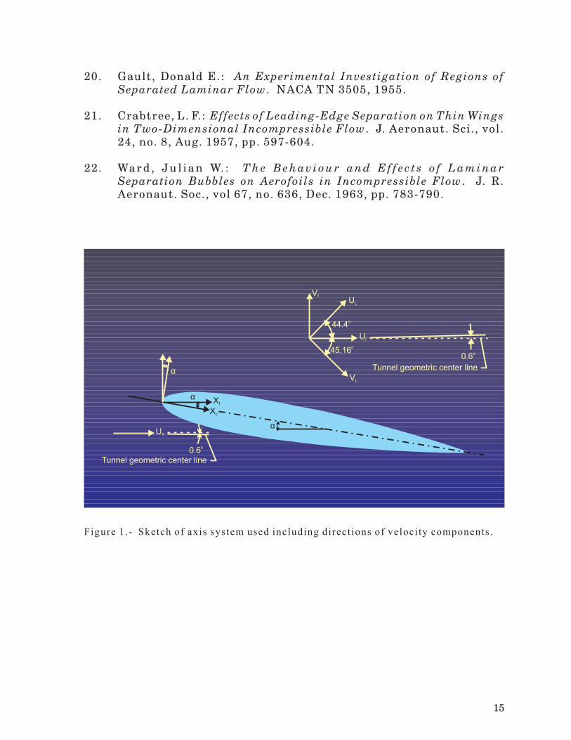
The axes used for this investigation are presented in figure 1. The unitsfor the physical quantities defined in this paper are in the InternationalSystem of Units (SI). Although most quantities were measured in thissystem, some were measured in U.S. Customary Units and converted byusing factors given in reference 17.

c wing chord, 0.3048 m

N number of velocity measurements in one ensemble

Ni

number of velocity measurements in ith histogram interval aspercent of N

U ,V local velocity components, direction described by subscript (seefig. 1)

UR local total velocity, U V

2 2 , m/sec

UT

free-stream velocity determined from pitot-static probe, m/sec

Xc,Y

ccoordinate axis relative to wing chord (fig. 1)

Xf,Y

fcoordinate axis relative to free stream (fig. 1)

xc

distance downstream from wing leading edge along chord, m

Yc

distance above and perpendicular to wing chord, m

α wing angle of attack, deg

Subscripts:

e ensemble-average data

f direction indication of parameters U , V , X , and Y parallel andperpendicular to free stream (see fig. 1)

i ith measurement in ensemble

L direction indication of velocity components inclined 44.4o abovefree stream and 45.6o below free stream (see fig. 1)

3

MODEL AND TEST TECHNIQUE

Apparatus

A fringe-type LV optics system operating in the backscatter mode wasused for the tests discussed in this report. This system was used tomeasure two components of velocity inclined 44.4

o

and -45.6o

to a planeparallel to the free stream, and utilized a Bragg cell to eliminatedirectional ambiguity problems as experienced in reference 1. A sketchof the optics system is presented in figure 2 and a photograph of thesystem is presented in figure 3. A high-speed burst counter was used tomeasure the period of the high-frequency signal contained in the burstfrom the particle traversing the sample volume. LV system control, dataacquisition, and data reduction were handled by a minicomputer. Ablock diagram of the data acquisition system is presented in figure 4. Acomplete description of the LV optical system, electronics system, anddata acquisition and reduction is available in reference 2.

The model used in this investigation was a simple straight wing. It had aspan of 2.438 m, a chord of 0.3048 m, and a NACA 0012 airfoil section.Ve l o c i t y m e a s u r e m e n t s w e r e m a d e a t m i d s p a n t o o b t a i n t w o -dimensional characteristics. The wing was supported by struts from thefloor near the tunnel center line and no balance measurements weretaken. The location of the strut mount to the wing was chosen as faroutboard as structurally feasible. This provided ample space betweenstruts to minimize f low disturbance at the wing center l ine . Aphotograph of the model with crossing laser beams is presented infigure 5.

Local flow velocities were measured about the wing center line at twoangles of attack, 0.6

o

and 4.75o

, to compare with theoretical predictions.A pitot-static probe was mounted 2.5 m below and 1 m ahead of the wingcenter line to provide accurate reference of the free-stream tunneld y n a m i c p r e s s u r e . A h y g r o m e t e r w a s u s e d t o o b t a i n w e t - b u l btemperatures; the total temperature was measured in the settlingchamber. Thus, the tunnel air density could be calculated and, withd y n a m i c p r e s s u r e m e a s u r e m e n t s , t h e t u n n e l v e l o c i t y c o u l d b eaccurately calculated.

Tunnel Seeding

Perhaps the foremost problem in achieving LV measurement accuracy isparticle lag. In most applications, the gas velocity distribution isdesired; however, the LV measures the velocity of seed particles in thegas. In many cases, these velocities are identical; however, in regions of

4

large velocity gradients, such as along a stagnation streamline, theinertia of larger particles does not allow them to adjust immediately tolocal flow velocity. Care is taken to ensure that the particles within theflow are small enough to follow the flow accurately. This problem wasaddressed in the investigation described in reference 1. It was foundt h a t 3 - µ m p a r t i c l e s r e s p o n d e d t o t h e s e v e r e v e l o c i t y g r a d i e n t(1540 m/sec per meter) along the stagnation line of a hemisphere at aMach number of 0.55.

Using this LV system, it was determined from laboratory tests andpre l iminary ca l cu lat ions that , a t the foca l l engths used in th isinvestigation, the minimum particle size for reasonable signal intensitywas on the order of 2 µm . This then put a 2- to 4-µm restriction on theparticle size required for practical use of the LV in the Langley V/STOLtunnel.

The smoke generator normally used in the V/STOL tunnel for flowvisual izat ion was modi f ied to yie ld the appropriate part ic le -s izedistribution for this test. This distribution was measured by an opticaltechnique similar to that discussed in reference 1 and is presented infigure 6(a). The smoke generator vaporized liquid kerosene by addingheat and emitted a dense white smoke through a nozzle. The nozzle waspositioned in the settling chamber of the tunnel to minimize flowdisturbance on the model. The nozzle position was critical in that theparticles were intended to be only in the area of the measurementvolume. The smoke plume in the test section was about 0.4 m indiameter. Any extensive movement of the sample volume resulted in itst ravers ing out o f the smoke p lume; thus , the nozz le had to berepositioned. This was done manually and was very time-consuming,requiring 20 to 60 min.

DATA ACQUISITION AND REDUCTION

Laser Velocimeter Data Processing

Statist ical quantit ies . - The LV measures velocity events that arePoisson distributed in time at a location in the flow. During themeasurement process, two assumptions are made. First, the particlesembedded in the flow are not only randomly dispersed in space but area l s o r a n d o m l y d i s p e r s e d i n t h e v e l o c i t y f i e l d ; a n d s e c o n d , t h emeasurement sample taken over a finite period of time is a goodrepresentat ion o f the s ta t ionary cond i t i on at the measurementlocation. The statistical quantities of sample mean and standarddeviation (and their statistical uncertainties), skew, and excess werecomputed. Graphical representat ions of the veloc i ty probabi l i ty

5

density functions for each of the velocity components were made byplacing each time-history sample of velocity measurements (ensemble)in histogram form and are presented in reference 2.

The sample mean was calculated by three different methods: (1)arithmetic mean, (2) arithmetic mean with corrections for velocity biasand Bragg cell bias (ref. 2), and (3) time averaging (ref. 18). An analysisof these methods is presented in reference 2. It was found in thisinvestigation that the three methods yielded similar results when themean data rate was above 10 particles per second. (See tables 2 to 4 inref. 2.) Thus, the statistical mean calculated from the test data wasdetermined by using the simple equation

VV

Ne

i=

Ins t rument prec i s i on . - The overa l l measurement prec i s i on wasobtained by determining the accuracies of all variables in the systemwhich would a f fec t the accuracy o f each ve loc i ty measurement .Reference 1 provides a complete description of the type of errorsinvolved in this investigation and of the error analysis method.

These errors yield an effective total bias error of -1.33 percent to0.91percent in velocity calculated by an algebraic sum of the partial biaserrors. The total effect of random error was ±0.47 percent uncertainty,which was obtained by taking the square root of the sum of the squares ofthe partial random errors described in reference 2.

In large velocity gradients, velocity measurement errors may occur ifthe measurement point is not at the desired locat ion. The two-component mechanical traversing system had a placement uncertaintyof ±1 mm, which yielded a worst case (based on the measured velocityflow field) uncertainty in velocity of 1.6percent due to position.

Particle Lag

Since the LV measures particle velocities and not the gas velocity, thefinal measurement accuracy is dependent on the ability of the particle tofollow the flow faithfully. The size distribution of the seed particle wasmeasured with an optical particle-size analyzer which was placed in thetest section to capture particles from the generator which yieldeda c c e p t a b l e LV s i g n a l s . T h e r e s u l t i n g d i s t r i b u t i o n i s s h o w n i nfigure 6(a). The particle size necessary for the LV to obtain validmeasurements was determined by using the computer simulation of the

6

LV developed by Meyers (ref. 19). The probability of a successfulmeasurement (ref. 2) as a funct ion of part ic le s ize is shown infigure 6(b). Thus, the overall measurement probability for this test wasfound (fig. 6 (c)). It was determined from reference 1 that a 3-µmparticle traveling at a free-stream Mach number of 0.55 would faithfullyfollow a velocity gradient of 1540 m/sec per meter. Since this velocitygradient is far greater than any obtained in the present tests, it isc o n c l u d e d t h a t t h e v e l o c i t y m e a s u r e m e n t s o b t a i n e d i n t h i sinvestigation are a true representation of the gas velocity flow field.

TEST AND PROCEDURES

This investigation was conducted in the Langley V/STOL tunnel at anominal free-stream Mach number of 0.15. The Reynolds number basedo n t h e w i n g c h o r d w a s a p p r o x i m a t e l y 1 x 1 0

6

. F r e e - s t r e a mmeasurements were made with the tunnel clear except for the pitot-static probe which was used as a reference. These measurements weremade in the vicinity where the model would be positioned. The wing wasinstalled at two angles of attack, 0.6

o

and 4.75o

.

The scan capability of this particular prototype LV system was notsufficient to survey above, ahead of, and behind the wing withoutmoving either the wing or the LV system platform. There was no surveybehind the wing at 0.6

o

angle of attack. With the wing at 4.75o

angle ofattack, a complete survey was made. To obtain the measurementsbehind the trailing edge, the model was moved forward and raised insidethe test section with very little change to the LV system platform.

To obtain measurements very near the leading edge and trailing edge ofthe model, the optical center line was inclined off-perpendicular to thetunnel such that the beam nearest the leading (or trailing) edge wasaligned with the edge. Thus, the angle of inclination of the opticalcenter line to the wing span was approximately 3

o

and parallel to thetunnel floor.

DISCUSSION

As ment ioned prev ious ly, a l l the ve loc i ty measurements at eachmeasurement location were first reduced to histogram form. Thesehistograms are presented in reference 2 with a figure list and a shortdiscussion of interpretation. Statistical analysis of the data wasperformed as described previously, and the results are presented intabulated form in reference 2.

7

Free-Stream Data

Preliminary analysis indicated that, at the Mach number used for thistest, the average flow angularity in the tunnel was 0.6

o

(inclined abovetunnel center line). The U

f, eand V

f, evelocities presented in this paper

are, therefore, referenced to free stream rather than tunnel center line.The freestream velocity computed from measurements by the pitot-s ta t i c probe U

Twas used to nondimens iona l i ze these ve loc i ty

components. Free-stream measurement comparison with the local totalvelocity U

Rindicated errors comparable to the combined pitot-static

probe and LV instrument error.

Basic Velocity Data for Wing at α = 4.75o

and 0.6o

Details of the statistical characteristics of the velocity data can be foundin reference 2. Some of these are summarized herein in the form ofcontour plots generated by using spline-fit routines between datapoints. These contour plots are presented in figures 7 to 10 for the wingat α = 4.75

o

and figures 11 to 14 for the wing at α = 0.6o

. The “arrow”plots (figs. 7 and 11) indicate the relative location of the velocitymeasurements and the magnitude and angle of the velocity vector.These plots, of course, were the matrix of data points used to generatethe contour plots. These arrow plots indicate the flow field to be whatone would expect about an airfoil at low angle of attack. The wake regionis definitely evident when α = 4.75

o

. The measurements near the leadingedge a t α = 4 .75

o

ind i ca te an unexpec ted phenomenon . Th i sphenomenon is discussed subsequently.

Streamlines (figs. 8 and 12) were generated by allowing a simulatedpar t i c l e to progress through the ve loc i ty - f i e ld matr ix that wasgenerated. The simulated particle responded to the velocity field as ittraversed the field. The path of the particle was stored and plotted on-line as a computed streamline. The phenomenon near the leading edgeof the wing at α = 4.75

o

is reflected in the streamline plots. Except fort h i s , t h e s e p l o t s a r e w h a t o n e w o u l d e x p e c t t o o b s e r v e u s i n gc o n v e n t i o n a l f l o w - v i s u a l i z a t i o n t e c h n i q u e s . L o c a l f l o w a n g l e spresented in this manner (figs. 9 and 13) indicate consistent andreasonable characteristics, except for the noted abnormality in theleading-edge region at α = 4.75

o

. Large local flow angles near the crest ofthe airfoil (25

o

at α = 4.75o

and 17o

at α = 0.6o

) were expected. The flowapproaches an angle tangent to the surface at the trailing edge. Thecontours of constant U

R/U

Tindicate the velocity decrease ahead of the

airfoil , an increase in velocity over the airfoil , and for the wing atα = 4.75

o

, a wake region with approximately 70 percent of the free-stream velocity,

8

Prediction Techniques

The external forces generated on a body in a fluid are manifested in thevelocity distribution of the fluid about the body. Accurate prediction ofthis velocity distribution can provide the researcher with a diagnostictool in interpret ing the results of more restr ict ive measurementtechniques. In developing such a prediction technique, a researcherverifies the prediction on the surface of the body with conventionalpressure measurements and force measurements . This has beenaccomplished for the two-dimensional viscous-flow prediction programand is reported in reference 15. Since the local surface pressures arecomputed from predicted local surface velocities, the off-body velocityprediction should be a very accurate measure of the flow phenomena asmeasured by the LV. The acceptability of the prediction technique as areference for the LV measurements is justified by the very accurateagreement with surface pressure measurements.

The theory for the two-dimensional viscous-flow prediction techniqueis well defined in reference 14 and will be described only in generalherein. It involves an iterative procedure which first obtains aninviscid-flow solution for the basic airfoil . A boundary-layer solution iscomputed based on the inviscid-flow solution, and a modified airfoil isthen constructed by adding the boundary-layer displacement thicknessto the original airfoil . The inviscid solution for the modified airfoil isobtained and the steps are then repeated until appropriate convergencecriteria are satisfied.

Since the wing in this case is not two-dimensional, a three-dimensionalflow program was used to determine the effect of three-dimensionalityat the center line of the wing. The prediction technique used for thiss tep i s an inv i sc id - f l ow pred i c t ion program and is descr ibed inreference 16. This method uses finite-strength vorticity distributionsinstead of concentrated-line vorticity on the body as is used by othercurrent methods. In this case, the wing was modeled by 160 panels.

Comparison of Experiment With Theory

The two LV-measured components of velocity rotated to the free-streamcoordinate system X

f,Y

fare presented in figures 15 to 33 for the wing at

α = 4.75o

and in figures 34 to 45 for the wing at α = 0.6o

. Each figurecorresponds to a scan perpendicular to the wing chord and can becoupled with the statistical characteristics plots and the histograms inre ference 2 . The ca l cu la ted ve loc i t i e s f rom the two pred i c t iont e c h n i q u e s a r e p r e s e n t e d i n e a c h f i g u r e f o r c o m p a r i s o n w i t hexperiment. The three-dimensional predicted velocities agree with the

9

two-dimensional predicted velocities within 2 percent except very nearthe airfoil surface. Thus, the assumption of two dimensionality at thecenter line of the wing is justified.

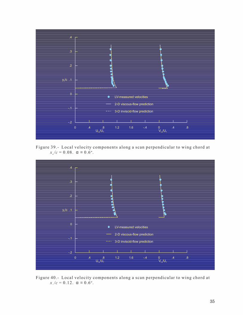
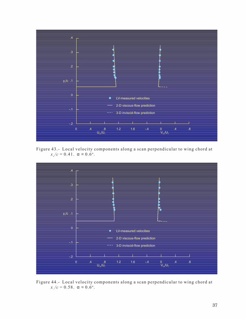
The theoretical predictions agree well with the LV-measured velocitiesfor the wing at α = 0.6

o

. The prediction technique is excellent above thewing and downstream of x

c/c = 0.08 (figs. 40 to 45). However, near the

leading edge and near the surface of the wing (fig. 37), the predictedvelocities are higher than the velocity field. Ahead of the wing (figs. 34to 36) , the pred ic t ion techniques prov ide a reasonably accurateassessment of the velocity field.

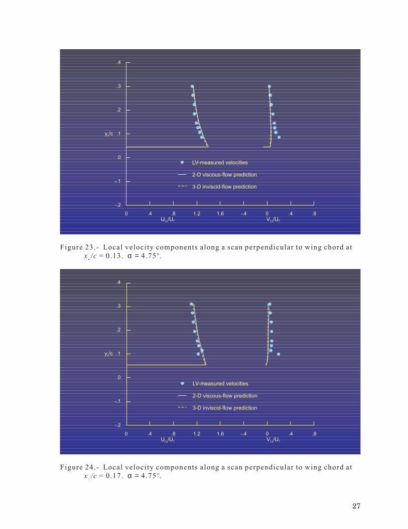
With the wing at α = 4.75o

, the prediction agrees only with the velocitymeasurements away from the surface and the lead ing edge . Atxc/c = –0.08 and -0.04 (figs. 16 and 17), the agreement is good until the

measurement location approaches the leading edge. At the leading edge( f ig . 18) the predicted veloc i t ies are higher than the measuredvelocities, and this discrepancy continues near the wing surface, atleast in the U

f, evelocity component, to chord position x

c/c = 0.13

(figs. 19 to 23). The Vf, e

velocity component is underestimated near thesurface to chord position x

c/c = 0.17 (figs. 19 to 24). The experimental

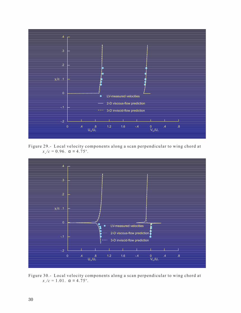
and theoretical velocity values are in good agreement farther aft of thischord position, except in the wake region, since the theory is inadequatein this region. (See figs. 30 to 33.) The wake profile is well defined withthe LV. The thickness of the wake is approximately 1.3 mm, which ismuch too small for conventional probes to measure without altering thecharacteristics of the wake.

The comparison of experiment and theory in this paper has been shownto be quite good except near the surface of the leading edge for the wingat α = 4.75

o

. This discrepancy is not an inadequacy of the predictionmethods , but a phenomenon of f low not modeled by the theory.Reference 2 indicated that double-peaked histograms at this locationwere evidence of a leading-edge laminar separation bubble. This bubbleexisted between the leading edge, along the upper surface, and trailingedge at α = 4.75

o

.

Samples of the histograms are presented in figures 46 and 47. Thehistograms are presented with a sketch of the wing cross section inwhich arrows indicate the position, direction, and relative magnitude ofthe mean velocity vectors. A run consisted of an ensemble of dataacquired at the position desired. The scan, therefore, was a series ofruns at various y

c/c positions at a constant chordwise position. The

histogram is a graphical representation of the variation of velocitymeasured over a time period. The histograms are presented with N

i, the

percentage of that number of measurements within an incremental

10

velocity band, as a function of velocity. In all cases, the UL

component ispresented on the left and the V

Lcomponent on the right. Interpretation

of histogram information is provided in appendix B of reference 2.

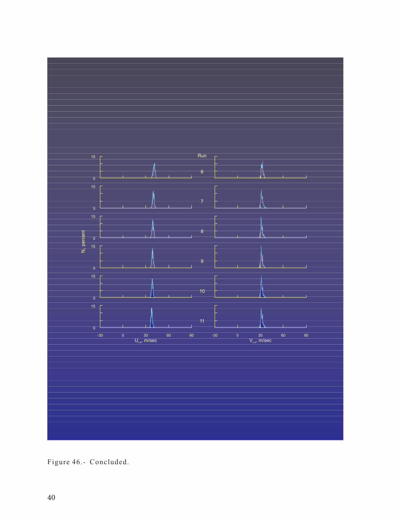
Figure 46 presents the histograms in a scan in which the predictiontechn iques agreed wi th the exper imenta l l y determined ve loc i tycomponents. (See fig. 15.) The histograms are well-defined Gaussian-type distributed velocity measurements with slight skew indicatingf luctuat ions in veloc i ty and angle as descr ibed in appendix B ofreference 2. Figure 47 presents the histograms in a scan in which thedouble peak appears, for example runs 50 to 52, which indicates thepresence of the shear layer. These double-peaked histograms indicatethat there are two predominant velocity values. The flow oscillatesbetween the two values and shows a tendency to be at or near one valueor the other, but spends little time between the two general values. TheV

L , ecomponent indicates that at the position for run 51, the flow is at

the lower velocity value most of the time; however at the position forrun 52, the flow is at the higher velocity value most of the time. Thepositions are only 0.007 chord lengths different in height (2.1 mm).These points are probably on opposite sides of the proposed shear layer.The most likely explanation of the double peak is that the shear layer isoscillatory. If the shear layer was steady, the double peaks wouldp r o b a b l y n o t e x i s t , a n d a s h i f t i n v e l o c i t y w o u l d o c c u r a s t h emeasurement location was traversed through it. This was believed to bean oscil lating shear layer from a laminar-separation bubble. Thelaminar separation bubble was justified by a similar situation reportedin reference 20. An NACA 0010 (modif ied) airfoi l was tested todetermine its characteristics when laminar separation was developed.Reference 20 indicates that at a Reynolds number of 1.5 x 10

6

at 4.75o

angle of attack, the NACA 0010 (modified) airfoil should have a laminarseparation at approximately x

c/c = 0.02, and the flow should make the

transition from laminar to turbulent and reattach at xc/c = 0.05.

Realizing that the present investigation of the NACA 0012 airfoil was ata Reynolds number of 1 x 10

6

at α = 4.75o

, it seems entirely possible thatthe phenomenon observed was a laminar-separation bubble. Theoscillation of the shear layer was justified by the skewed histogramsahead of this point on the airfoil . A skewed histogram, as explained inappendix B of reference 2, indicates a fluctuation primarily in flowangle. Thus, the flow was experiencing variations in velocity and angle.T h e p o s i t i o n o f t h e l a m i n a r - s e p a r a t i o n p o i n t a s m e a s u r e d i nreference 20 was found to be highly sensitive to slight wing angle-of-attack changes; therefore, it is possible that the separation point wasmoving with the flow-angle oscillation. This unsteadiness in separationpoint would result in unsteadiness in the shear layer of the separationand trigger an undulating shear layer.

11

References 21 and 22 provide an analysis of the effects of the separationbubble on airfoils. Reference 21 in particular indicates that localsurface velocities just ahead of the bubble are lower than those withoutthe bubble. The local surface velocities downstream are increased bythe presence of the bubble, and if the bubble reattaches, the velocitiesapproach those of the airfoil without the bubble. The data presented inreference 2 are summarized in figure 48 and indicate similar trends;that is, ahead of the airfoil and the proposed laminar-separation bubble,the theoretical ly computed velocit ies (without laminar-separationbubble) are higher than the experimentally measured velocities (withlaminar-separation bubble). Figure 48 indicates that downstream ofxc/c = 0.7 the experimental values are larger than the theoretical

values, and at the trailing edge the velocities compare favorably. Thiswould indicate, based on the analysis in reference 22, that the bubblebegan near the leading edge and reattached downstream.

CONCLUDING REMARKS

An analyt ica l invest igat ion was conducted using two methods todetermine the flow field at the center line of an unswept wing with anaspect ratio of eight. The analysis used a two-dimensional viscous-flowpred ic t ion technique for the f low- f i e ld ca l cu lat ion and a three -dimensional potential-flow panel method to evaluate the degree of two-dimensionality achieved at the wing center line.

The three-dimensional potential-flow program results differed verylittle from the two-dimensional viscous-flow program results (outsidethe boundary layer), which indicates essentially two-dimensional flowconditions at the measurement location.

The agreement between experiment and these theories indicated thatboth the theoretical techniques and the experiment provided truerepresentations of the velocity field about the airfoil .

Measurements within the very small wake region of this airfoil wereobtained and indicated a typical velocity defect.

The data for the wing at α = 4.75o

indicated that a laminar-separationbubble probably existed with a thin osci l lat ing shear layer. Theprediction technique did not model this bubble; therefore, in the area ofthe bubble, the correlation was poor.

Langley Research CenterNational Aeronautics and Space AdministrationHampton, VA 23665 March 15, 1978

12

REFERENCES

1. Young, Warren H., Jr.; Meyers, James F.; and Hepner, Timothy E.:Laser Velocimeter Systems Analysis Applied to a Flow SurveyAbove a Stalled Wing. NASA TN D-8408, 1977.

2. Hoad, Danny R.; Meyers, James F.; Young, Warren H., Jr.; andHepner, Timothy E.: Laser Velocimeter Survey About a NACA 0012Wing at Low Angles of Attack. NASA TM-74040, 1978.

3. Meyers, James F.; Feller, William V.; and Hepner, Timothy E.: AFeasibility Test of the Laser Velocimeter in the Mach 5 Nozzle TestChamber . Proceedings of the Second International Workshop onLaser Velocimetry, Volume I, H. D. Thompson and W. H. Stevenson,eds., Eng. Exp. Stn. Bull. No. 144, Purdue Univ., 1974, pp. 290-313.

4. Whiff en, M. C.; and Meadows, D. M.: Two Axis, Single ParticleL aser Velocimeter System for Turbulence Spectral Analysis .Proceedings of the Second International Workshop on LaserVelocimetry, Volume I, H. D. Thompson and W. H. Stevenson, eds.,Eng. Exp. Stn. Bull. No. 144, Purdue Univ., 1974, pp. 1-15.

5. Egg ins , P. L . ; and Jackson , D. A . : L aser-Dopp l e r Ve lo c i t yMeasurements in an Under-Expanded Free Jet . J. Phys. D: Appl.Phys., vol. 7, no. 14, Sept. 21, 1974, pp. 1894-1906.

6. Goldman, Louis J.; Seasholtz, Richard G.; and McLallin, Kerry L.:Velocity Surveys in a Turbine Stator Annular-Cascade FacilityUsing Laser Doppler Techniques . NASA TN D-8269, 1976.

7. Wilson, John C.: A General Rotor Model System for Wind-TunnelInvestigations . J. Aircr., vol. 14, no. 7, July 1977, pp. 639-643.

8. Sullivan, John P.: An Experimental Investigation of Vortex Ringsand Helicopter Rotor Wakes Using a Laser Doppler Velocimeter .T e c h . R e p . N o . 1 8 3 ( C o n t r a c t N o . N 0 0 0 1 9 - 7 2 - C - 0 4 5 0 ) ,Massachusetts Inst. Technol., June 1973. (Available from DDC asAD 778 768.)

9. Johnson, Bruce V.: LDV Measurements in the Periodic VelocityField Adjacent to a Model Helicopter Rotor . Proceedings of theSecond International Workshop on Laser Velocimetry, Volume II,H. D. Thompson and W. H. Stevenson, eds., Eng. Exp. Stn. Bull.No. 144, Purdue Univ., 1974, pp. 169-181.

13

10. Landgrebe, Anton J.; and Johnson, Bruce V.: Measurement ofModel Helicopter Rotor Flow Velocities With a Laser DopplerVelocimeter . J. American Helicopter Soc., vol. 19, no. 3, July 1974,pp. 39-43.

11. Biggers, James C.; and Orloff, Kenneth L.: Laser VelocimeterMeasurements of the Helicopter Rotor-Induced Flow Field . J.American Helicopter Soc., vol. 20, no. 1, Jan. 1975, pp. 2-10.

12. Hsieh, Tsuying: Analysis of Veloci ty Measurements About aHemisphere-Cylinder Using a Laser Velocimeter . J. Spacecr. &Rockets, vol. 14, no.,5, May 1977, pp. 280-283.

13. Meyers, James F.; Couch, Lana M; Feller, William V.; and Walsh,Michael J.: Laser Velocimeter Measurements in a Large TransonicWind Tunnel . Minnesota Symposium on Laser Anemometry -Proceedings, E. R. G. Eckert, ed., Univ. of Minnesota, Oct. 1975,pp. 84-111.

14. Smetana, Frederick O.; Summey, Delbert C.; Smith, Neill S.; andCarden, Ronald K. : Light Aircraf t Lif t , Drag, and MomentPrediction - A Review and Analysis . NASA CR-2523, 1975.

15. M c G h e e , R o b e r t J. ; a n d B e a s l e y, Wi l l i a m D. : L o w - S p e e dAerodynamic Characteristics of a 17-Percent-Thick Airfoil SectionDesigned for General Aviation Applications . NASA TN D-7428,1973.

16. Hess, John L.: Calculation of Potential Flow About ArbitraryThree-Dimensional Lif t ing Bodies . Rep. No. MDC J5679-01(Contract N00019-71-C-0524), McDonnell Douglas Corp., Oct.1972. (Available from DDC as AD 755 480.)

17. Mechtly, E. A.: The International System of Units - PhysicalConstants and Conversion Factors (Second Revision) . NASA SP-7012, 1973.

18. Yule, G. Udny; and Kendall, M. G.: An Introduction to theTheory of Statistics . Charles Griffin & Co., Ltd., 1940.

19. Meyers, James F.; and Walsh, Michael J.: Computer Simulation ofa Fringe Type Laser Velocimeter . Proceedings of the SecondInternational Workshop on Laser Velocimetry, Volume I, H. D.Thompson and W. H. Stevenson, eds., Eng. Exp. Stn. Bull. No. 144,Purdue Univ., 1974, pp. 471-510.

14

20. Gault, Donald E.: An Experimental Investigation of Regions ofSeparated Laminar Flow . NACA TN 3505, 1955.

21. Crabtree, L. F.: Effects of Leading-Edge Separation on Thin Wingsin Two-Dimensional Incompressible Flow . J. Aeronaut. Sci. , vol.24, no. 8, Aug. 1957, pp. 597-604.

22. Wa r d , J u l i a n W. : T h e B e h a v i o u r a n d E f f e c t s o f L a m i n a rSeparation Bubbles on Aerofoils in Incompressible Flow . J. R.Aeronaut. Soc., vol 67, no. 636, Dec. 1963, pp. 783-790.

Figure 1.- Sketch of axis system used including directions of velocity components.

15

Vf

UL

44.4o

Uf

45.16o

VL

Tunnel geometric center line

0.6o

Tunnel geometric center line

0.6o

UT

Xc

Xf

α

α

α

Figure 2.- Schematic of laser velocimeter optics.

Figure 3.- Laser velocimeter optics platform in Langley V/STOL tunnel.

16

TunnelWindow

Traversing System

Mirrors

Argon ion Laser

Mirrors

Mirrors

Photo-multiplier

TubeSpatialFilter

FocusingLensBragg Cell

Optical Switch

Beam SplitterLens

Negative Lens

Figure 4.- Block diagram of laser velocimeter data-acquisi t ion system.

Figure 5.- NACA 0012 wing installed in Langley V/STOL tunnel.

17

PhotomultiplierTube

High-speedBurst Counter Optical Traverse

System

Optical ScanController

CRT Terminal

Line Printer

Plotter

15-MbyteDisk

Minicomputer

Laser VelocimeterAutocorrelation

Buffer

PhotomultiplierTube

High-speedBurst Counter

9-trackMagnetic Tape

Figure 6.- Part icle-size and probabil i ty distr ibutions measured by laser velocimeter.

18

0 1 2 3 4 5

Diameter of seed particle, microns

(c) Overall measurement probability1.0

0.5

0

(b) Probability of successful measurement.1.0

0.5

0

1.0

0.5

0

(a) Particulate size distribution.

Pro

babili

tydis

trib

ution

function

(norm

aliz

ed

topeak

am

plit

ude)

Figure 7.- Velocity vectors computed from measurements over wing at α = 4.75 o .

Figure 8.- Streamlines computed from interpolated flow-angle distr ibution over wing

at α = 4.75 o .

19

Figure 9.- Contours of constant local flow angle measured over wing at α = 4.75 o .

Figure 10.- Contours of constant UR , e /UT measured over wing at α = 4.75 o .

20

5

5

5 5

6

6

7

10

1520

25

4 3 2 10 -1

-2 -3 -4

-4

-5

-6

-7

-7

-6

-5

-5

-4

-4

-3-3

-7

-6

-8

.85.9.95

.95

1.0

1.05 1.10 1.151.15

1.2

1.2

1.251.3

1.1

1.1 1.05

1.0

.95

.9

.9

.7

1.05

1.0

1.0

.95

Figure 11.- Velocity vectors computed from measurements over wing at α = 0.6 o .

Figure 12.- Streamlines computed from interpolated flow-angle distr ibution over wing

at α = 0.6 o .

21

Figure 13.- Contours of constant local flow angle measured over wing at α = 0.6 o .

Figure 14.- Contours of constant UR , e /UT measured over wing at α = 0.6 o .

22

1

2

3

17 161412109

87

3

4

5

6

3 2 1

00

-3

0 -1

-2

-3

.825.85

.875

.90

.925

.95

.975

1.0

1.0251.05

1.075

1.1251.15

1.175

1.05

1.10

Figure 15.- Local velocity components along a scan perpendicular to wing chord at

x c /c = -0.16. α = 4.75 o .


x c /c = -0.08. α = 4.75 o .

23

.8.40-.41.61.2.8.40V /Uf,e TU /Uf,e T

-.2

-.1

0

.1

.2

.3

.4

y /cc

LV-measured velocities

2-D viscous-flow prediction

3-D inviscid-flow prediction

.8.40-.41.61.2.8.40V /Uf,e TU /Uf,e T

-.2

-.1

0

.1

.2

.3

.4

y /cc





x c /c = -0.04. α = 4.75 o .


x c /c = 0. α = 4.75 o .

24




.8.40-.41.61.2.8.40V /Uf,e TU /Uf,e T

-.2

-.1

0

.1

.2

.3

.4

y /cc

.8.40-.41.61.2.8.40V /Uf,e TU /Uf,e T

-.2

-.1

0

.1

.2

.3

.4

y /cc




.8.40-.41.61.2.8.40V /Uf,e TU /Uf,e T

-.2

-.1

0

.1

.2

.3

.4

y /cc


x c /c = 0.03. α = 4.75 o .


x c /c = 0.04. α = 4.75 o .

25




.8.40-.41.61.2.8.40V /Uf,e TU /Uf,e T

-.2

-.1

0

.1

.2

.3

.4

y /cc




.8.40-.41.61.2.8.40V /Uf,e TU /Uf,e T

-.2

-.1

0

.1

.2

.3

.4

y /cc


x c /c = 0.06. α = 4.75 o .


x c /c = 0.09. α = 4.75 o .

26




.8.40-.41.61.2.8.40V /Uf,e TU /Uf,e T

-.2

-.1

0

.1

.2

.3

.4

y /cc




.8.40-.41.61.2.8.40V /Uf,e TU /Uf,e T

-.2

-.1

0

.1

.2

.3

.4

y /cc


x c /c = 0.13. α = 4.75 o .


x c /c = 0.17. α = 4.75 o .

27




.8.40-.41.61.2.8.40V /Uf,e TU /Uf,e T

-.2

-.1

0

.1

.2

.3

.4

y /cc




.8.40-.41.61.2.8.40V /Uf,e TU /Uf,e T

-.2

-.1

0

.1

.2

.3

.4

y /cc


x c /c = 0.29. α = 4.75 o .


x c /c = 0.42. α = 4.75 o .

28




.8.40-.41.61.2.8.40V /Uf,e TU /Uf,e T

-.2

-.1

0

.1

.2

.3

.4

y /cc




.8.40-.41.61.2.8.40V /Uf,e TU /Uf,e T

-.2

-.1

0

.1

.2

.3

.4

y /cc


x c /c = 0.58. α = 4.75 o .


x c /c = 0.75. α = 4.75 o .

29




.8.40-.41.61.2.8.40V /Uf,e TU /Uf,e T

-.2

-.1

0

.1

.2

.3

.4

y /cc




.8.40-.41.61.2.8.40V /Uf,e TU /Uf,e T

-.2

-.1

0

.1

.2

.3

.4

y /cc


x c /c = 0.96. α = 4.75 o .


x c /c = 1.01. α = 4.75 o .

30




.8.40-.41.61.2.8.40V /Uf,e TU /Uf,e T

-.2

-.1

0

.1

.2

.3

.4

y /cc

.8.40-.41.61.2.8.40V /Uf,e TU /Uf,e T

-.2

-.1

0

.1

.2

.3

.4

y /cc





x c /c = 1.03. α = 4.75 o .


x c /c = 1.09. α = 4.75 o .

31

.8.40-.41.61.2.8.40V /Uf,e TU /Uf,e T

-.2

-.1

0

.1

.2

.3

.4

y /cc




.8.40-.41.61.2.8.40V /Uf,e TU /Uf,e T

-.2

-.1

0

.1

.2

.3

.4

y /cc





x c /c = 1.13. α = 4.75 o .


x c /c = -0.17. α = 0.6 o .

32

.8.40-.41.61.2.8.40V /Uf,e TU /Uf,e T

-.2

-.1

0

.1

.2

.3

.4

y /cc




.8.40-.41.61.2.8.40V /Uf,e TU /Uf,e T

-.2

-.1

0

.1

.2

.3

.4

y /cc





x c /c = -0.09. α = 0.6 o .


x c /c = -0.05. α = 0.6 o .

33

.8.40-.41.61.2.8.40V /Uf,e TU /Uf,e T

-.2

-.1

0

.1

.2

.3

.4

y /cc




.8.40-.41.61.2.8.40V /Uf,e TU /Uf,e T

-.2

-.1

0

.1

.2

.3

.4

y /cc





x c /c = 0. α = 0.6 o .


x c /c = 0.04. α = 0.6 o .

34

.8.40-.41.61.2.8.40V /Uf,e TU /Uf,e T

-.2

-.1

0

.1

.2

.3

.4

y /cc




.8.40-.41.61.2.8.40V /Uf,e TU /Uf,e T

-.2

-.1

0

.1

.2

.3

.4

y /cc





x c /c = 0.08. α = 0.6 o .


x c /c = 0.12. α = 0.6 o .

35

.8.40-.41.61.2.8.40V /Uf,e TU /Uf,e T

-.2

-.1

0

.1

.2

.3

.4

y /cc




.8.40-.41.61.2.8.40V /Uf,e TU /Uf,e T

-.2

-.1

0

.1

.2

.3

.4

y /cc





x c /c = 0.16. α = 0.6 o .


x c /c = 0.29. α = 0.6 o .

36

.8.40-.41.61.2.8.40V /Uf,e TU /Uf,e T

-.2

-.1

0

.1

.2

.3

.4

y /cc




.8.40-.41.61.2.8.40V /Uf,e TU /Uf,e T

-.2

-.1

0

.1

.2

.3

.4

y /cc





x c /c = 0.41. α = 0.6 o .


x c /c = 0.58. α = 0.6 o .

37

.8.40-.41.61.2.8.40V /Uf,e TU /Uf,e T

-.2

-.1

0

.1

.2

.3

.4

y /cc




.8.40-.41.61.2.8.40V /Uf,e TU /Uf,e T

-.2

-.1

0

.1

.2

.3

.4

y /cc





x c /c = 0.70. α = 0.6 o .

38

.8.40-.41.61.2.8.40V /Uf,e TU /Uf,e T

-.2

-.1

0

.1

.2

.3

.4

y /cc




Figure 46.- Histograms in scan at x c /c = -0.16. α = 4.75 o .

39

Run

123456789

1011

15

0

Run

1

15

0

2

15

0

3

15

0

4

15

0

5

-30 0 30 60 90 -30 0 30 60 90

U , m/secL,e V , m/secL,e

N,

pe

rce

nt

i

Figure 46.- Concluded.

40

15

0

Run

6

15

0

7

15

0

8

15

0

9

15

0

10

15

0

11

-30 0 30 60 90 -30 0 30 60 90


N,

pe

rce

nt

i

Figure 47.- Histograms in scan at x c /c = 0. α = 4.75 o .

41

Run4344454647484950515253

15

0

Run

43

15

0

44

15

0

45

15

0

47

-30 0 30 60 90 -30 0 30 60 90


15

0

46

N,

pe

rce

nt

i

Figure 47.- Concluded.

42

15

0

Run

48

15

0

49

15

0

50

15

0

51

15

0

52

15

0

53

-30 0 30 60 90 -30 0 30 60 90


N,perc

ent

i

Figure 48.- Local total velocity comparison with theory at constant heights above wing.

α = 4.75 o .

43

1.4

1.3

1.2

1.1

1.0

.9

.8

U /UR,e T

-.2 -.1 0 .1 .2 .3 .4 .5 .6 .7 .8 .9 1.0 1.1 1.2

x /cc

.06c above wing surface

1.4

1.3

1.2

1.1

1.0

U /UR,e T


1.4

1.3

1.2

1.1

1.0

U /UR,e T


1.4

1.3

1.2

1.1

1.0

U /UR,e T


LV-measured velocities2-D viscous-flow prediction

Date post:	03-Feb-2022
Category:	Documents
Upload:	others
View:	6 times
Download:	0 times

1978 Correlation of Laser Velocimeter Measurments Over a Wing.pdf

Documents