1996, Vol. 11, No. 4, 283{319 Bioequivalence Trials ...

Statistical Science1996, Vol. 11, No. 4, 283–319

Bioequivalence Trials, Intersection–UnionTests and Equivalence Confidence SetsRoger L. Berger and Jason C. Hsu

Abstract. The bioequivalence problem is of practical importance be-cause the approval of most generic drugs in the United States and theEuropean Community (EC) requires the establishment of bioequivalencebetween the brand-name drug and the proposed generic version. Theproblem is theoretically interesting because it has been recognized asone for which the desired inference, instead of the usual significant dif-ference, is practical equivalence. The concept of intersection–union testswill be shown to clarify, simplify and unify bioequivalence testing. Atest more powerful than the one currently specified by the FDA and ECguidelines will be derived. The claim that the bioequivalence problemdefined in terms of the ratio of parameters is more difficult than theproblem defined in terms of the difference of parameters will be refuted.The misconception that size-α bioequivalence tests generally correspondto 100�1 − 2α�% confidence sets will be shown to lead to incorrect sta-tistical practices, and should be abandoned. Techniques for constructing100�1−α�% confidence sets that correspond to size-α bioequivalence testswill be described. Finally, multiparameter bioequivalence problems willbe discussed.

Key words and phrases: Bioequivalence; bioavailability; hypothesis test;confidence interval; intersection–union; size; level; equivalence test;pharmacokinetic; unbiased.

1. BIOEQUIVALENCE PROBLEM

Two different drugs or formulations of the samedrug are called bioequivalent if they are absorbedinto the blood and become available at the drug ac-tion site at about the same rate and concentration.Bioequivalence is usually studied by administeringdosages to subjects and measuring concentration ofthe drug in the blood just before and at set timesafter the administration. These data are then usedto determine if the drugs are absorbed at the samerate.

The determination of bioequivalence is very im-portant in the pharmaceutical industry becauseregulatory agencies allow a generic drug to be mar-keted if its manufacturer can demonstrate that the

Roger L. Berger is Professor, Department of Sta-tistics, North Carolina State University, Raleigh,North Carolina 27695-8203 (e-mail: [email protected]). Jason C. Hsu is Professor, Departmentof Statistics, Ohio State University, Columbus, Ohio43210-1247 (e-mail: [email protected]).

generic product is bioequivalent to the brand-nameproduct. The assumption is that bioequivalentdrugs will provide the same therapeutic effect. Ifthe generic drug manufacturer can demonstratebioequivalence, it does not need to perform costlyclinical trials to demonstrate the safety and effi-cacy of the generic product. Yet, this bioequivalencemust be demonstrated in a statistically sound wayto protect the consumer from ineffective or unsafedrugs.

These concentration by time measurements areconnected with a polygonal curve and several vari-ables are measured. The common measurementsare AUC (area under curve), Cmax (maximumconcentration) and Tmax (time until maximum con-centration). The two drugs are bioequivalent if thepopulation means of AUC and Cmax are sufficientlyclose. Descriptive statistics for Tmax are usuallyprovided, but formal tests are not required.

For example, let µT denote the population meanAUC for the generic (test) drug and let µR denotethe population mean AUC for the brand-name (ref-erence) drug. To demonstrate bioequivalence, the

283

284 R. L. BERGER AND J. C. HSU

following hypotheses are tested:

H0xµTµR≤ δL or

µTµR≥ δU

(1) versus

Hax δL <µTµR

< δU:

The values δL and δU are standards set by regula-tory agencies that define how “close” the drugs mustbe to be declared bioequivalent. Currently, both theUnited States Food and Drug Administration (FDA,1992a) and the European Community use δU = 1:25and δL = 0:80 = 1/1:25 for AUC. For Cmax, theUnited States again uses δU = 1:25 and δL = 0:80,but Europe uses the less restrictive limits δU = 1:43and δL = 0:70 = 1/1:43 (Hauck et al., 1995). Notethat these limits for AUC and Cmax are symmetricabout 1 in the ratio scale.

Often, logarithms are taken and hypotheses (1)are stated as

H0x ηT − ηR ≤ θL or ηT − ηR ≥ θU(2) versus

Hax θL < ηT − ηR < θU:

Here, ηT = log�µT�, ηR = log�µR�, θU = log�δU�and θL = log�δL�. With δU = 1:25 and δL = 0:80or δU = 1:43 and δL = 0:70, θU = −θL, and thestandards are symmetric about zero.

In a hypothesis test of (1) or (2), the Type I errorrate is the probability of declaring the drugs to bebioequivalent, when in fact they are not. By settingup the hypotheses as in (1) or (2) and controllingthe Type I error rate at a specified small value, say,α = 0:05, the consumer’s risk is being controlled.That (1) or (2) is the proper formulation in problemslike these was recognized early on by some authors.For example, Lehmann (1959, page 88), not specifi-cally discussing bioequivalence, says, “One then setsup the (null) hypothesis that [the parameter] doesnot lie within the required limits so that an error ofthe first kind consists in declaring [the parameter]to be satisfactory when in fact it is not.” But not un-til Schuirmann (1981, 1987a), Westlake (1981) andAnderson and Hauck (1983) were hypotheses cor-rectly formulated as in (1) or (2) in bioequivalenceproblems.

Despite the fact that bioequivalence testing prob-lems are now correctly formulated as (1) or (2),many inappropriate statistical procedures are stillused in this area. Tests that claim to have a spec-ified size α, but are either liberal or conservative,

are used. Liberal tests compromise the consumer’ssafety, and conservative tests put an undue burdenon the generic drug manufacturer. Tests are oftendefined in terms of confidence intervals in statis-tically unsound ways. These tests, again, do notproperly control the consumer’s risk.

In this paper, we will describe current bioequiva-lence tests that have incorrect error rates. We willoffer new tests that correctly control the consumer’srisk. In several cases, the tests we propose are uni-formly more powerful than the existing tests whilestill controlling the Type I error rate at the speci-fied rate α. We will examine and criticize the cur-rent practice of defining tests in terms of 100�1 −2α�% confidence sets. We will show that this onlyworks in special cases and gives poor results inother cases. We will discuss how properly to con-struct 100�1 − α�% confidence sets that correspondto size-α tests. And we will discuss how our methodscan be applied to complicated, multiparameter bioe-quivalence problems that have received only slightattention in the literature. The intersection–unionmethod of testing will be found to be very usefulin understanding and constructing bioequivalencetests. Section 2 provides a more detailed outline ofour discussions.

Hypotheses such as (1) and (2) that specify onlythat population means should be close are calledaverage bioequivalence hypotheses. Hypotheses thatstate that the whole distribution of bioavailabilitiesis the same for the test and reference populationsare called population bioequivalence hypotheses. Ifa parametric form of these populations is assumed,then hypotheses such as (25) that specify that allpopulation parameters (e.g., variances as well asmeans) should be close are population bioequiva-lence hypotheses. Sometimes bioequivalence is de-fined in terms of parameters that more directly mea-sure equivalence of response within an individual.Good introductions to individual bioequivalence aregiven by Anderson and Hauck (1990), Hauck andAnderson (1992), Sheiner (1992), Schall and Luus(1993) and Anderson (1993). Although we do notexplicitly consider individual bioequivalence in thispaper, many of the concepts and techniques we de-scribe should be applicable in that area also.

In this paper, our discussion will be entirely interms of bioequivalence testing. But our commentsand techniques apply to other problems, such asin quality assurance, in which the aim is to showthat two parameters are close or that a parame-ter is between two specification limits. Because ofthis wider applicability, the methods we will discussmight more properly be referred to as equivalencetests and equivalence confidence intervals.

BIOEQUIVALENCE TRIALS 285

2. TESTS, CONFIDENCE SETSAND CURIOSITIES

Various experimental designs are used to gatherdata for bioequivalence trials. Chow and Liu (1992)describe parallel designs (two independent samples)and two-period and multiperiod crossover designs.The issues we discuss apply to all these differentdesigns. For brevity, we will discuss only the simpleparallel design and two period crossover design.

2.1 Difference Hypotheses

It is customary to employ lognormal models inbioequivalence studies of AUC and Cmax. See Sec-tion 2.2 for rationales for this model.

LetX∗ denote a lognormal measurement from thetest drug in the original scale, and let X = log�X∗�.Similarly, let Y∗ denote an original measurement,and let Y = log�Y∗� for the reference drug. Let�ηT; σ2� denote the lognormal parameters for X∗

and �ηR; σ2� denote the lognormal parameters forY∗. Then the test and reference drug means areµT = exp�ηT + σ2/2� and µR = exp�ηR + σ2/2�, re-spectively. Therefore, the condition

δL <µTµR= exp�ηT − ηR� < δU

is equivalent to

θL < ηT − ηR < θU;(3)

where θL = log�δL� and θU = log�δU� are knownconstants. Thus, the hypothesis to be tested in thislognormal model can be stated as either (1) or (2).Usually the hypotheses are stated as (2) and thetest is based on log transformed data that is nor-mally distributed with means ηT and ηR and com-mon variance σ2. The equivalence of (1) and (2) isdependent on the assumption of equal variances. Onthe other hand, if µT and µR represent the mediansof X∗ and Y∗ and ηT = log�µT� and ηR = log�µR�,then ηT and ηR are the medians of X and Y, re-spectively. So, in terms of medians, (1) and (2) are al-ways equivalent, and the analysis can be carried outin either the original or log transformed scale. But,bioequivalence is almost always defined in terms ofmeans rather than medians.

Westlake (1981) and Schuirmann (1981) proposedwhat has become the standard test of (2). It is calledthe “two one-sided tests” (TOST). The TOST has thisgeneral form. Let D be an estimate of ηT −ηR thathas a normal distribution with mean ηT − ηR andvariance σ2

D. Let SE�D� be an estimate of σD that isindependent of D and such that r�SE�D��2/σ2

D hasa χ2 distribution with r degrees of freedom. Then

t = D− �ηT − ηR�SE�D�

has a Student’s t-distribution with r degrees of free-dom. The TOST is based on the two statistics

TU =D− θUSE�D� and TL =

D− θLSE�D� :(4)

The TOST tests (2) using the ordinary, one-sided,size-α t-test based on TL for

H01x ηT − ηR ≤ θL(5) versus

Ha1x ηT − ηR > θLand the ordinary, one-sided, size-α t-test based onTU for

H02x ηT − ηR ≥ θU(6) versus

Ha2x ηT − ηR < θU:It rejects H0 at level α and declares the two drugsto be bioequivalent if both tests reject, that is, if

TU < −tα; r and TL > tα; r;(7)

where tα; r is the upper 100α percentile of a Stu-dent’s t-distribution with r degrees of freedom. Fortesting (2), all the tests we will discuss are func-tions of �D;SE�D��. The distribution of �D;SE�D��is determined by the parameter �ηT; ηR; σ2

D�.In the simple parallel design, let X∗1; : : : ;X

∗m

denote the independent lognormal �ηT; σ2� mea-surements on m subjects from the test drug inthe original scale, and let X1; : : : ;Xm denote thelogarithms of these measurements. Similarly, letY∗1; : : : ;Y

∗n and Y1; : : : ;Yn denote the original

measurements [lognormal�ηR; σ2�� and logarithmsfor an independent sample of n subjects on thereference drug. If X denotes the sample meanof X1; : : : ;Xm, Y denotes the sample mean ofY1; : : : ;Yn and S2 denotes the pooled estimate ofσ2, computed from both samples, then

D =X−Yand

SE�D� = S√

1m+ 1n:

The degrees of freedom are r =m+ n− 2.In bioequivalence studies, much more com-

mon than simple parallel designs are two-period,crossover designs. In a two-period, crossover de-sign, a group of m subjects (Sequence 1) receivesthe reference drug and observations on the phar-macokinetic response are made. After a washoutperiod to remove any carryover effect, this groupreceives the test drug and observations are again


made. A second group of n subjects (Sequence 2)receives the drugs in the opposite order. After logtransformation, the response of the kth subject inthe jth period of the ith sequence is modeled as

Yijk = γ +Sik +Pj +F�i; j� + εijk;where γ is the overall mean; Pj is the fixed effectof period j; F�i; j� is the fixed effect of the formu-lation administered in period j of sequence i, thatis, F�1;1� = F�2;2� = FR and F�1;2� = F�2;1� = FT;Sik is the random effect of subject k in sequencei; and εijk is the random error. It is assumed thatP1 + P2 = FT + FR = 0. The Sik’s and the εijk’sare all independent normal random variables withmean 0. The variance of Sik is σ2

S and the varianceof εijk is σ2

T and σ2R for the test and reference for-

mulations, respectively. For this design,

D = Y12• −Y11• +Y21• −Y22•2

is a normally distributed unbiased estimate of FT−FR = ηT − ηR with variance

σ2D = �σ2

R + σ2T�

14

(1m+ 1n

):

The standard error of D is

SE�D� = S12

√1m+ 1n;

where

S2 = 1m+ n− 2

·[ m∑k=1

(Y12k −Y11k − �Y12• −Y11•�

)2

+n∑k=1

(Y21k −Y22k − �Y21• −Y22•�

)2]:

The estimate D is the average of the averages ofthe intrasubject differences for the two sequences,and S2 is a pooled estimate of the variance of an in-trasubject difference. For this crossover design, also,the degrees of freedom are r =m+ n− 2.

Following Lehmann (1959), we define the size ofa test as

size = supH0

P�reject H0�:

The size of the TOST is exactly equal to α, eventhough P�reject H0� < α for every �ηT; ηR; σ2

D� inthe null hypothesis. The supremum value of α is at-tained in the limit as ηT − ηR = θL (or θU) andσ2D → 0. Both the FDA bioequivalence guideline

(FDA, 1992a) and the European Community guide-line (EC-GCP, 1993) specify that bioequivalence beestablished using a 5% TOST.

The TOST is unusual in that two size-α tests arecombined to form a size-α test. Often, when multi-ple tests are combined, some adjustment must bemade to the sizes of the individual tests to achievean overall size-α test. Why this is not necessary forthe TOST is best understood through the theory ofintersection–union tests (IUT’s), which we describein Section 3. In Sections 4.1 and 4.2 we will showthat the IUT theory is useful for understanding theTOST. Also, the IUT theory can guide the construc-tion of tests for (2) that have the same size α as theTOST but are uniformly more powerful than theTOST.

2.2 Ratio Hypotheses

Sometimes, a normal model should be used. Inthis model, the original measurements are normallydistributed with means µT and µR. This model isdifferent from the lognormal model in that now thehypothesis to be tested concerns the ratio of themeans of these normal observations. That is, wewish to test (1). This problem has received less at-tention than (2). Dealing with the ratio µT/µR hasbeen perceived as more difficult than dealing withthe difference ηT − ηR.

For AUC and Cmax, the FDA (1992a) stronglyrecommends logarithmically transforming the dataand testing the hypotheses (2). They offer three ra-tionales for their recommendation. Based on these,the FDA (1992a, page 7) states:

Based on the arguments in the precedingsection, the Division of Bioequivalencerecommends that the pharmacokineticparameters AUC and Cmax be log trans-formed. Firms are not encouraged to testfor normality of data distribution af-ter log transformation, nor should theyemploy normality of data distributionas a justification for carrying out thestatistical analysis on the original scale.

The emphasis is ours.The FDA’s three rationales for log transformation

are labeled “Clinical,” “Pharmacokinetic” and “Sta-tistical.” The Clinical Rationale is that the real in-terest is in the ratio µT/µR rather than the differ-ence µT−µR. But, the link between this fact (whichwe certainly do not dispute) and the log transfor-mation of the data is based on statistical considera-tions. It is that a linear statistical model can be usedfor the transformed data to make inferences aboutthe difference ηT−ηR. These inferences then can berestated in terms of µT/µR. Thus, the justificationof the log transformations seems to be based mainlyon the perceived difficulty in dealing with the ratio


µT/µR, rather than the difference ηT−ηR. If appro-priate statistical procedures can be used to make in-ferences about the ratio µT/µR directly, then thereseems to be no need for a log transformation.

The Pharmacokinetic Rationale is based on multi-plicative compartmental models of Westlake (1973,1988). The multiplicative model is changed to a lin-ear model by the log transformation. Part of theStatistical Rationale is that, in the original scale,much bioequivalence data is skewed and appearsmore lognormal than normal. We agree that thesetwo considerations suggest that the first method ofanalysis to be considered in bioequivalence studiesis on the log transformed data, and, in most cases,this analysis will be appropriate.

The Statistical Rationale consists of the previouslognormal justification and two more points. Thefirst is that:

Standard parametric methods are ill-suited to making inferences about theratio of two averages, though some validmethods do exist. Log transformationchanges the problem to one of making in-ferences about the difference (on the logscale) of the two averages, for which thestandard methods are well suited.

The second is that the small sample sizes used intypical bioequivalence studies (20–30) will producetests for normality that have fairly low power ineither the original or log scale. The FDA recom-mends that no check of normality be made on thelog transformed data. But, if a low-power normalitytest rejects the hypothesis of normality for the logtransformed data, then surely some caution is war-ranted in the use of procedures that assume nor-mality. In this case, tests such as the TOST, basedon the Student’s t-distribution, are inappropriate.If normality of the log transformed data is rejectedand the original data appear more normal than thelog transformed data, then procedures that assumenormality of the original data would seem more ap-propriate. In Section 4.3, we show that Sasabuchi(1980,1988a,b) described the size-α likelihood ratiotest for (1). It is a simple test based on the Stu-dent’s t-distribution. So the FDA’s statement aboutill-suited standard parametric procedures seems un-founded. We also show that the tests commonly usedare liberal and have size greater than the nomi-nal value of α. Furthermore, we show that the IUTmethod can be used in this problem, also, to con-struct size-α tests that are uniformly more power-ful than the likelihood ratio test. Thus, the FDA’savoidance of (1) because of statistical difficulties isunwarranted.

An alternative test, when normality is in doubt,might be to use a Wilcoxon–Mann–Whitney ana-logue of the TOST [based on the original loga-rithmically transformed data for a parallel design,or the intrasubject between-period differences ofthe logarithmically transformed data, as proposedby Hauschke, Steinijans and Diletti (1990), for acrossover design].

2.3 100(1 2 2a)% Confidence Intervals

One would expect the TOST to be identical tosome confidence interval procedure: for some ap-propriate 100�1− α�% confidence interval �D−;D+�for ηT − ηR, declare the test drug to be bioequiva-lent to the reference drug if and only if �D−;D+� ⊂�θL; θU�.

It has been noted (e.g., Westlake, 1981;Schuirmann, 1981) that the TOST is operationallyidentical to the procedure of declaring equivalenceonly if the ordinary 100�1− 2α�%, not 100�1− α�%,two-sided confidence interval for ηT − ηR,

�D− tα; rSE�D�;D+ tα; rSE�D��;(8)

is contained in the interval �θL; θU�. In fact, bothFDA (1992a) and EC-GCP (1993) specify that theTOST should be executed in this fashion.

The fact that the TOST seemingly corresponds toa 100�1−2α�%, not 100�1−α�%, confidence intervalprocedure initially caused some concern (Westlake,1976, 1981). Recently, Brown, Casella and Hwang(1995) called this relationship an “algebraic coin-cidence.” But many authors (e.g., Chow and Shao,1990, and Schuirmann, 1989) have defined bioequiv-alence tests in terms of 100�1−2α�% confidence sets.

Standard statistical results, such as Theorems 3and 4 in Section 5, give relationships between size-αtests and 100�1 − α�% confidence intervals. In Sec-tion 5, we discuss a 100�1−α�% confidence intervalthat corresponds exactly to the size-α TOST. We alsoexplore the relationship between 100�1− 2α�% con-fidence intervals and size-α tests. We describe situ-ations more general than the TOST in which size-αtests can be defined in terms of 100�1− 2α�% confi-dence intervals. But we also give examples from thebioequivalence literature of tests that have been de-fined in terms of 100�1− 2α�% confidence intervalsand sets that are not size-α tests. Tests defined by100�1− 2α�% confidence intervals can be either lib-eral or conservative. Because of these potential diffi-culties, our conclusion is that the practice of definingbioequivalence tests in terms of 100�1− 2α�% confi-dence intervals should be abandoned. If both a confi-dence interval and a test are required, a 100�1−α�%confidence interval that corresponds to the givensize-α test should be used.


2.4 Multiparameter Problems

In Section 6, we discuss multiparameter bioequiv-alence problems. We discuss two examples in whichthe IUT theory can be used to define size-α teststhat are uniformly more powerful than tests thathave been previously proposed. These examplesconcern controlling the experimentwise error ratewhen several parameters are tested for equivalence,simultaneously.

3. INTERSECTION–UNION TESTS

Berger (1982) proposed the use of intersection–union tests in a quality control context closelyrelated to bioequivalence testing. Tests for manydifferent bioequivalence hypotheses are easily con-structed using the IUT method. The TOST is asimple example of an IUT. Tests with a specifiedsize are easily constructed using this method, evenin complicated problems involving several param-eters. And tests that are uniformly more powerfulthan standard tests can often be constructed usingthis method.

The IUT method is useful for the following typeof hypothesis testing problem. Let θ denote the un-known parameter (θ can be vector valued) in the dis-tribution of the data X. Let 2 denote the parameterspace. Let 21; : : : ; 2k denote subsets of 2. Supposewe wish to test

H0x θ ∈k⋃i=1

2i versus Hax θ ∈k⋂i=1

2ci;(9)

where Ac denotes the complement of the set A. Theimportant feature in this formulation is the null hy-pothesis is expressed as a union and the alterna-tive hypothesis is expressed as an intersection. Fori = 1; : : : ; k, let Ri denote a rejection region for atest of H0ix θ ∈ 2i versus Haix θ ∈ 2ci . Then anIUT of (9) is the test that rejects H0 if and only ifX ∈ ⋂k

i=1Ri. The rationale behind an IUT is sim-ple. The overall null hypothesis, H0x θ ∈

⋃ki=12i,

can be rejected only if each of the individual nullhypotheses, H0ix θ ∈ 2i, can be rejected.

Berger (1982) proved the following two theorems.

Theorem 1. If Ri is a level-α test of H0i, for i =1; : : : ; k, then the intersection–union test with rejec-tion regionR = ⋂k

i=1Ri is a level-α test of H0 versusHa in (9).

An important feature in Theorem 1 is that eachof the individual tests is performed at level-α, butthe overall test also has the same level α. There isno need for multiplicity adjustment for performingmultiple tests. The reason there is no need for such a

correction is the special way the individual tests arecombined. Hypothesis H0 is rejected only if everyone of the individual hypotheses, H0i, is rejected.

Theorem 1 asserts that the IUT is level-α. Thatis, its size is at most α. In fact, a test constructedby the IUT method can be quite conservative. Itssize can be much less than the specified value α.However, Theorem 2 (a generalization of Theorem2 in Berger, 1982) provides conditions under whichthe IUT is not conservative; its size is exactly equalto the specified α.

Theorem 2. For some i = 1; : : : ; k, suppose Ri isa size-α rejection region for testing H0i versus Hai.For every j = 1; : : : ; k; j 6= i, suppose Rj is a level-αrejection region for testing H0j versus Haj. Supposethere exists a sequence of parameter points θl; l =1;2; : : : ; in 2i such that

liml→∞

Pθl�X ∈ Ri� = α

and, for every j = 1; : : : ; k; j 6= i,liml→∞

Pθl�X ∈ Rj� = 1:

Then the intersection–union test with rejection re-gion R = ⋂k

i=1Ri is a size-α test of H0 versus Ha.

Note that in Theorem 2 the one test defined byRi has size exactly α. The other tests defined byRj; j = 1; : : : ; k; j 6= i, are level-α tests. That is,their sizes may be less than α. The conclusion is theIUT has size α. Thus, if rejection regions R1; : : : ;Rk

with sizes α1; : : : ; αk are combined in an IUT andTheorem 2 is applicable, then the IUT will havesize equal to maxi�αi�. We will discuss bioequiva-lence examples in which tests of different sizes arecombined. The resulting test has size equal to themaximum of the individual sizes.

4. OLD AND NEW TESTS FOR DIFFERENCEAND RATIO HYPOTHESES

4.1 Two One-Sided Tests

The TOST is naturally thought of as an IUT. Thebioequivalence alternative hypothesis Hax θL <ηT − ηR < θU is conveniently expressed as theintersection of the two sets,

2c1 = ��ηT; ηR; σ2D�x ηT − ηR > θL�

and

2c2 = ��ηT; ηR; σ2D�x ηT − ηR < θU�:

The test that rejects H01x ηT − ηR ≤ θL in (5) ifTL ≥ tα; r is a size-α test ofH01. The test that rejectsH02x ηT − ηR ≥ θU in (6) if TU ≤ −tα; r is a size-α


test of H02. So, by Theorem 1, the test that rejectsH0 only if both of these tests reject is a level-α testof (2).

To use Theorem 2 to see that the size of the TOSTis exactly α, consider parameter points with ηT −ηR = θU and take the limit as σ2

D → 0. Such pa-rameters are on the boundary of H02. Therefore,

P�X ∈ R2� = P�TU ≤ −tα; r� = α;for any σ2

D > 0. But,

P�X ∈ R1� = P�TL ≥ tα; r� → 1 as σ2D→ 0;

because the power of a one-sided t-test converges to1 as σ2

D → 0 for any point in the alternative. Thevalue ηT − ηR = θU is in the alternative, Ha1.

The advantage of considering bioequivalenceproblems in an IUT format is not limited to verify-ing properties of the TOST. Rather, other bioequiv-alence hypotheses, such as (1), state an intervalas the alternative hypothesis. This interval canbe expressed as the intersection of two one-sidedintervals. So two one-sided, size-α tests can be com-bined to obtain a level-α (typically, size-α) test.Furthermore, as we will see in Section 6, evenmore complicated forms of bioequivalence can beexpressed in the IUT format. This allows the easyconstruction of tests with guaranteed size-α forthese problems.

4.2 More Powerful Tests

Despite its simplicity and intuitive appeal, theTOST suffers from a lack of power. The line labeledTOST in the top part of Table 1 shows the powerfunction, P�reject H0�, for parameter points withηT − ηR = θU (or θL), points on the boundary be-tween H0 and Ha. The power function is near αfor σ2

D near 0, but decreases as σ2D grows. An unbi-

ased test would have power equal to α for all suchparameter points. The TOST is clearly biased. The

Table 1Powers of three bioequivalence tests; r = 30, α = 0:05 and θU =

log�1:25� = −θL

σD

0.00 0.04 0.08 0.12 0.16 0.20 0.30 ∞

ηT − ηR = θU or θLTOST 0.050 0.050 0.050 0.031 0.003 0.000 0.000 0.000BHM 0.050 0.050 0.050 0.050 0.050 0.050 0.050 0.050New 0.050 0.050 0.050 0.047 0.049 0.050 0.050 0.050

ηT − ηR = 0TOST 1.000 1.000 0.720 0.158 0.007 0.000 0.000 0.000BHM 1.000 1.000 0.721 0.260 0.131 0.093 0.066 0.050New 1.000 1.000 0.720 0.247 0.128 0.092 0.066 0.050

bottom part of Table 1 shows the power functionwhen the two drugs are exactly equal, ηT = ηR. Thepower is near 1 for σ2

D near 0, but decreases to 0 asσ2D increases. Despite these shortcomings, Diletti,

Hauschke and Steinijans (1991) declared that theTOST maximizes the power among all size-α tests.This is incorrect.

Anderson and Hauck (1983) proposed a test withhigher power than the TOST. Whereas the TOSTdoes not reject H0 if SE�D� is sufficiently large, theAnderson and Hauck test always rejects H0 if D isnear enough to 0, even if SE�D� is large. This pro-vides an improvement in power. However, the An-derson and Hauck test does not control the Type Ierror probability at the specified level α. It is liberaland the size is somewhat greater than α. Shortlyafter Anderson and Hauck proposed their test, Pa-tel and Gupta (1984) and Rocke (1984) proposedthe same test. This scientific coincidence was com-mented upon by Anderson and Hauck (1985) andMartin Andres (1990).

Due to the seriousness of a Type I error, declar-ing two drugs to be equivalent when they are not,the search for a size-α test that was uniformly morepowerful than the TOST continued. Munk (1993)proposed a slightly different test. Munk claims thatthis test is a size-α test that is uniformly more pow-erful than the TOST, but this claim is supported bynumerical calculations, not analytic results.

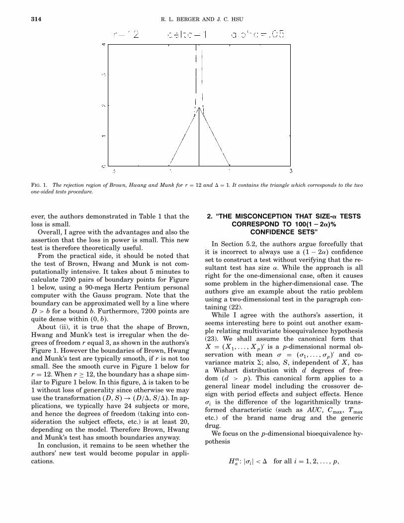
Brown, Hwang and Munk (1995) constructed anunbiased, size-α test of (2) that is uniformly morepowerful than the TOST. Their construction is re-cursive. To determine if a point �d; se�D�� is in therejection region of the Brown, Hwang and Munktest, a good deal of computing can be necessary. Thismay limit the practical usefulness of the Brown,Hwang and Munk test. Also, sometimes the Brown,Hwang and Munk rejection region has a quite irreg-ular shape. An example of this is shown in Figure 1.

We will now describe a new test of the hypotheses(2). This test is uniformly more powerful than theTOST. Unlike the Anderson and Hauck and Munktests, our test is a size-α test. Our test is nearlyunbiased. It is simpler to compute than the Brown,Hwang and Munk test. It will not have the irregu-lar boundaries that the Brown, Hwang and Munktest sometimes possesses. The construction of thisnew test again illustrates the usefulness of the IUTmethod.

To simplify the notation in describing our test, weassume, without loss of generality, that θL = −θUand we call θU = 1. Following Brown, Hwang andMunk, define S2

∗ = r�SE�D��2. It is simpler to defineour test in terms of the polar coordinates, centered


Fig. 1. Irregular boundary of Brown, Hwang and Munk test�solid line� and smoother boundary of test from Section 4:2�dashed line�; the TOST rejection region is bounded by the tri-angle with vertices at −1; 1 and T. Here r = 3; α = 0:16 and−θL = θU = 1:

at �1;0�,v2 = �d− 1�2 + s2

∗

and

b = cos−1 ��d− 1�/v� :In the �d; s∗� space, v is the distance from �1;0� to�d; s∗� and b is the angle between the d axis and theline segment joining �1;0� and �d; s∗�. To define asize-α test, we need the distribution of �V;B� whenθ = 1. In this case, it is easy to verify that V andB are independent. The probability density functionof B is

f�b� = 0��r+ 1�/2�0�r/2�√π �sin�b��r−1; 0 < b < π;

which does not depend on σ2D. To implement our

test, it is useful to note that the cumulative distri-bution function of B has a closed form given by

F�b� = b

π− 1

2√π

·�r−1�/2∑k=1

�sin�b��2k−1 cos�b� 0�k�0�k+ �1/2�� ;

if r is odd, and

F�b� = 12− 1

2√π

r/2∑k=1

�sin�b��2k−2 cos�b�0�k− �1/2��0�k� ;

if r is even. The probability density function of Vwill be denoted by gσD�v�.

We will describe the rejection region of the newtest geometrically here. Exact formulas are in the

Appendix. The new test will be an IUT. We will de-fine a size-α, unbiased rejection region, R2, for test-ing (6). This R2 will contain the rejection regionof the size-α TOST and will be approximately sym-metric about the line d = 0. Then we will defineR1 = ��d; s∗�x �−d; s∗� ∈ R2�; R1 is R2 reflectedacross the line d = 0; R1 is a size-α, unbiased rejec-tion region for testing (5). Then R = R1 ∩R2 is therejection region of the new test. Because R2 is ap-proximately symmetric about the line d = 0, R1 isalmost the same as R2, and not much is deletedwhen we take the intersection. This foresight inchoosing the individual rejection regions so that theintersection is not much smaller is always usefulwhen using the IUT method.

The set �V = v� is a semicircle in �d; s∗� space.For each value of v, R2�v� ≡ �V = v� ∩R2 is eitherone or two intervals of b values, that is, one or twoarcs on �V = v�. These arcs will be chosen so that,for every v > 0,

∫R2�v�

f�b�db = α:(10)

Then the rejection probability

P�R2� =∫ ∞

0

∫R2�v�

f�b�dbgσD�v�dv

=∫ ∞

0αgσD�v�dv = α;

for every σD > 0 if ηT − ηR = 1. This will ensurethat R2 is a size-α, unbiased rejection region fortesting (6).

We now define the arc(s) that make up R2�v�. Re-fer to Figure 2 in this description. The rejection re-gion of the size-α TOST, call it RT, is the trian-gle bounded by the lines s∗ = 0, d = 1 − tα; rs∗/

√r

(call this line lU) and d = −1 + tα; rs∗/√r (call this

Fig. 2. Arcs that define the rejection region R2.


line lL). Let v0 denote the distance from �1;0� tolL. In this description, we assume 1/2 > α > α∗ ≡1 − F�3π/4�. Brown, Hwang and Munk (1995) intheir Table 1 show that if r ≥ 4, then α = 0:05 > α∗.The new test for α ≤ α∗ is given in the Appendix.Brown, Hwang and Munk did not propose any testfor α ≤ α∗. The condition α > α∗ ensures that thepoint on lL closest to �1;0� is on the boundary ofRT, as shown.

Let b0 denote the angle between the d-axis andlU. For 0 < v ≤ v0, R2�v� = �bx b0 < b < π�. The arcA0 in Figure 2 is an example of such an arc. So, forv < v0, R2�v� is exactly the points in the TOST.

For v0 < v, the semicircle V = v intersects lLat two points. Let b1 < b2 denote the angles corre-sponding to these two points. If v0 < v < 21, letA2�v� = �bx b2 < b < π�. These are the points inRT adjacent to the d-axis, and A2 in Figure 2 is anexample of such an arc. If 21 ≤ v, let A2�v� be theempty set. Let α�v� denote the probability contentof A2�v� under F. That is,

α�v� ={

1−F�b2�; v0 < v < 21;0; 21 ≤ v:

For v0 < v, R2�v� = A1�v�∪A2�v�, where, to ensurethat (10) is true, A1�v� must satisfy

∫A1�v�

f�b�db = α− α�v�:(11)

Let �d1; s∗1� denote the point where the �V = v0�semicircle intersects lU, and let v1 denote the radiuscorresponding to �−d1; s∗1�. For v0 < v < v1, let bL1be the angle defined by

F�b1� −F�bL1� = α− α�v�;(12)

where b1 is as defined in the previous paragraph.Then A1�v� = �bx bL1 < b < b1� is the arc that sat-isfies (11) whose endpoint is on lL. For v0 < v < v1,R2�v� = A1�v� ∪A2�v�, using this A1�v�. The arcslabeled A1 and A2 in Figure 2 comprise such anR2�v�. For v < v1, the cross sections R2�v� we havedefined are the same as the cross sections for theBrown, Hwang and Munk (1995) test. They now de-fine the remainder of their rejection region recur-sively in terms of these arcs. We define our rejectionregion in a nonrecursive manner.

For v1 ≤ v, define two values bL�v� < bU�v� suchthat F�bU�v�� −F�bL�v�� = α− α�v�, and the anglebetween the line joining �0;0� and �v; bL�v�� and thes∗-axis is the same as the angle between the linejoining �0;0� and �v; bU�v�� and the s∗-axis. Thisequal angle condition is what we meant earlier bythe phrase “approximately symmetric about the lined = 0.” If bU�v� ≥ b1, then A1�v� = �bx bL�v� < b <bU�v��. But, if bU�v� < b1, then this arc does not

contain all the points in the TOST. So, if bU�v� < b1,A1�v� = �bx bL1 < b < b1�, where bL1 is defined by(12). For v1 ≤ v, R2�v� = A1�v� ∪ A2�v�. Recall,if 21 ≤ v, A2�v� is empty, and R2�v� is the singlearc A1�v�. Also, for v2 ≥ max�412; 12 + 12r/t2α; r�,the semicircle �V = v� does not intersect RT, andR2�v� is the arc defined by bL�v� and bU�v�. Theb1-condition never applies in this case. In Figure 2,the solid parts of the arcs A3 and A4 are examplesof R2�v� for v1 ≤ v.

The cross sections R2�v� have been defined forevery v > 0, and this defines R2; R1 is the reflectionof R2 across the s∗-axis, and the rejection region ofthe new test is R = R1 ∩ R2. This construction isillustrated in Figure 3.

In Figure 1, the rejection region R with the samesize as the Brown, Hwang and Munk test is theregion between the dotted lines. The boundary ofR is smooth compared to the irregular boundaryof the Brown, Hwang and Munk test. This smooth-ness results from the attempt in the construction ofR to center arcs around the s∗-axis. To determineif a sample point �d; s2

∗� is in R, two arcs, R2�v�and R1�v� = R2�v′� (v′ = �−d − 1�2 + s2

∗, computedfrom �−d; s2

∗�), must be constructed. If �d; s2∗� is on

both arcs, �d; s2∗� ∈ R. But, to determine if �d; s2

∗�is in the rejection region of the Brown, Hwang andMunk test, a starting point is selected. Then a se-quence of arcs is constructed until �d; s2

∗� is passed.Then another sequence of arcs is constructed froma new starting point. This process is continued un-til enough arcs in the vicinity of �d; s2

∗� are obtainedto approximate the boundary of the rejection region.From this it is determined if �d; s2

∗� is in the rejec-tion region. Thus, a good deal more computation is

Fig. 3. Rejection region of new test; region R2 �between solidlines� and region R1 �between dashed lines); rejection region R =R1 ∩R2; r = 10 and α = 0:05.


needed to implement the Brown, Hwang and Munktest. Also, the Brown, Hwang and Munk test is notdefined for α ≤ α∗. This smoothness, general appli-cability and simplicity of computation recommendsR as a reasonable alternative to the Brown, Hwangand Munk test. But R is slightly biased whereas theBrown, Hwang and Munk test is unbiased.

A small power comparison of the TOST, Brown,Hwang and Munk test and our new test is given inTable 1 for α = 0:05 and r = 30. In the top blockof numbers, ηT − ηR = 1. For these boundary val-ues, the power is exactly α = 0:05 for the unbi-ased Brown, Hwang and Munk test. The power isalso very close to 0.05 for our test, indicating it hasonly slight bias. But the TOST is highly biased withpower much less than 0.05 for moderate and largeσD. In the bottom block of numbers, ηT − ηR = 0.The drugs are equivalent. Our test and the Brown,Hwang and Munk test have very similar powers.Their powers are much greater than the TOST’spower for all but small σD. For example, it canbe seen that the power improvement is about 60%when σD = 0:12 and about 85% when σD = 0:16.Sample sizes for bioequivalence tests are often cho-sen so that the test has power of about 0.8 whenηT = ηR. In this case, Table 1 indicates there is noadvantage to using the new tests over the TOST.But if the variability turns out to be larger thanexpected in the planning stage, the new tests offersignificant power improvements.

The tests of Anderson and Hauck (1983), Brown,Hwang and Munk (1995) and our new test all havethe property that, as s∗→∞, the width of the rejec-tion region increases, eventually containing valuesof �d; s∗� with d outside the interval �θL; θU�. Therewill be values �d; s∗1� and �d; s∗2� with s∗1 < s∗2,but �d; s∗1� is not in the rejection region while�d; s∗2� is in the rejection region. This “flaring out”of the rejection region is evident in Figures 1 and5 (see Section A.2). This counterintuitive shapewas pointed out by Rocke (1984). The rejection re-gion of any bioequivalence test that is unbiased, orapproximately unbiased, must eventually containsample points with d outside the interval �θL; θU�.Some have suggested that such procedures shouldbe truncated in the sense that the narrowest pointof the rejection region be determined and then therejection region is extended along the s∗-axis only ofthis width. Brown, Hwang and Munk suggest thisas a possible modification of their test, although theresulting test will no longer be unbiased. We be-lieve that notions of size, power and unbiasednessare more fundamental than “intuition” and do notrecommend truncation. But for those who disagree,our new test could be truncated in this same way.

The narrowest point will need to be determinednumerically for all these tests, and the smoothershape of our rejection region will make this deter-mination easier. Referring to Figure 1, a numericalroutine might be fooled by the irregular shape ofthe Brown, Hwang and Munk test.

4.3 Tests for Ratios of Parameters

Usually, data from a bioequivalence trial is loga-rithmically transformed before analysis. This leadsto a test of the hypotheses (2), as described in theprevious section. In the model we will considernow, the original data are normally distributed.Let X1; : : : ;Xm form a random sample from a nor-mal population with mean µT and variance σ2, andlet Y1; : : : ;Yn form an independent random sam-ple from a normal population with mean µR andvariance σ2. In this section, we will present ourcomments in terms of this simple parallel design.Yang (1991) and Liu and Weng (1995) describe mod-els for this normally distributed data in crossoverexperiments.

The bioequivalence hypothesis to be tested in thiscase is (1), namely,

H0xµTµR≤ δL or

µTµR≥ δU

(13) versus

Hax δL <µTµR

< δU:

In the past, the values of δL = 0:80 and δU = 1:20were commonly used (called the ±20 rule). However,the FDA Division of Bioequivalence (FDA, 1992a)now uses δL = 0:80 and δL = 1:25. These limits aresymmetric about 1 in the ratio scale since 0:80 =1/1:25.

The parameter µR is positive because the mea-sured variable, AUC or Cmax, is positive. Thereforethe hypotheses (13) can be restated as

H0x µT − δLµR ≤ 0 or µT − δUµR ≥ 0

(14) versus

Hax µT − δLµR > 0 and µT − δUµR < 0:

The testing problem (14) was first considered bySasabuchi (1980, 1988a, b). Let X, Y and S2 de-note the two sample means and the pooled estimateof σ2. Sasabuchi showed that the size-α likelihoodratio test of (14) rejects H0 if and only if

T1 ≥ tα; r and T2 ≤ −tα; r;where

T1 =X− δLY

S√

1/m+ δ2L/n


and

T2 =X− δUY

S√

1/m+ δ2U/n

:

This will be called the T1/T2 test.The T1/T2 test is easily understood as an IUT.

The usual, normal theory, size-α t-test of H01x µT −δLµR ≤ 0 versus Ha1x µT − δLµR > 0 is the testthat rejects H01 if T1 ≥ tα; r. Similarly, the usual,normal theory, size-α t-test of H02x µT − δUµR ≥ 0versus Ha2x µT − δUµR < 0 is the test that rejectsH02 if T2 ≤ −tα; r. Because Ha is the intersectionof Ha1 and Ha2, these two t-tests can be combined,using the IUT method, to get a level-α test of H0versus Ha. Using an argument like that in Section4.1, Theorem 2 can be used to show that the size ofthis test is α.

Yang (1991) and Liu and Weng (1995) proposedtests closely related to the T1/T2 test for the bioe-quivalence problem of testing (13) in a crossover ex-periment. Hauck and Anderson (1992) also discussthe hypotheses in the form (14), but no reference toSasabuchi’s earlier work is given. The derivation ofthe confidence set for µT/µR in Hsu, Hwang, Liuand Ruberg (1994) contains a mistake in the stan-dardization. Properly corrected, their rather com-plicated confidence set would lead to the rejection of(14) when the simple test described above does. So,somehow, the value of this simple, size-α test seemsto have been completely overlooked in the bioequiv-alence literature. Rather, Chow and Liu (1992) andLiu and Weng (1995) both report that the follow-ing is the standard analysis. Rewrite the hypotheses(13) or (14) as

H0x µT − µR ≤ �δL − 1�µRor µT − µR ≥ �δU − 1�µR

versus

Hax �δL − 1�µR < µT − µR < �δU − 1�µR:

(15)

These hypotheses look like (2), but there is an im-portant difference. In (2), θL and θU are knownconstants. In (15), �δL − 1�µR and �δU − 1�µR areunknown parameters. Nevertheless, the standardanalysis proceeds to use the TOST with �δL − 1�Yreplacing θL in TL and �δU − 1�Y replacing θU inTU. The standard analysis ignores the fact that aconstant has been replaced by a random variableand compares these two test statistics to standardt-percentiles as in the TOST. This test will be calledthe T∗1/T

∗2 test.

The statistics that are actually used in this anal-ysis are

T∗1 =X−Y− �δL − 1�YS√

1/m+ 1/n

= X− δLYS√

1/m+ 1/n= T1

√n+mδ2

L

n+m ;

and

T∗2 =X−Y− �δU − 1�YS√

1/m+ 1/n

= X− δUYS√

1/m+ 1/n= T2

√n+mδ2

U

n+m :

The statistics T1 and T2 are properly scaled tohave Student’s t-distributions, but T∗1 and T∗2 arenot. The T∗1/T

∗2 test is an IUT in which the two

tests have different sizes. The test that rejects H01if T∗1 > tα; r has size

PµT=δLµR(T∗1 > tα; r

)

= PµT=δLµR(T1 >

√n+mn+mδ2

L

tα; r

)

= α1 < α;

because√

n+mn+mδ2

L

> 1:

On the other hand, the test that rejects H02 if T∗2 <−tα; r has size

PµT=δUµR(T∗2 < −tα; r

)

= PµT=δUµR(T2 < −

√n+mn+mδ2

U

tα; r

)

= α2 > α;

because√

n+mn+mδ2

U

< 1:

Theorem 2 can be used to show that, as a test of thehypothesis (13), the T∗1/T

∗2 test has size α2 > α. It

is a liberal test.The true size of the T∗1/T

∗2 test, for a nominal size

of α = 0:05, is shown in Table 2. In Table 2 it isassumed that the sample sizes from the test andreference drugs are equal, m = n. In this case, thesize of the T∗1/T

∗2 test is simply

α2 = P(T < −

√2

1+ δ2U

tα; r

);


Table 2Actual size of T∗1/T

∗2 test for nominal α = 0:05

m = n 5 10 15 20 30 ∞

Size 0.070 0.071 0.072 0.072 0.073 0.073

whereT has a Student’s t-distribution with r = 2n−2 degrees of freedom. It can be seen that the size ofthe T∗1/T

∗2 test is about 0.07 for all sample sizes.

The liberality worsens slightly as the sample sizeincreases. On the other hand, the T1/T2 test hassize exactly equal to the nominal α. It is just assimple to implement as the T∗1/T

∗2 test. Therefore

the T1/T2 test should replace the T∗1/T∗2 test for

testing (13).In Section 4.2, the IUT method was used to con-

struct a size-α test that is uniformly more power-ful than the TOST. For the known σ2 case, Berger(1989) and Liu and Berger (1995) used the IUTmethod to construct size-α tests that are uniformlymore powerful than the T1/T2 test. In Figure 4,the cone-shaped region labeled R0 is the rejectionregion of the T1/T2 test for α = 0:05. The regionbetween the dashed lines is the rejection region ofLiu and Berger’s size-α test that is uniformly morepowerful. We refer the reader to Berger (1989) andLiu and Berger (1995) for the details about thesetests. We believe that, for the case of σ2 unknown,size-α tests that are uniformly more powerful thanthe T1/T2 test will be found.

Fig. 4. Rejection region for T1/T2 test is cone shaped R0; regionbetween dashed lines is rejection region of uniformly more pow-erful Liu and Berger �1995� test. The estimates X and Y satisfyδL < X/Y < δU in the larger cone-shaped region.

5. CONFIDENCE SETS ANDBIOEQUIVALENCE TESTS

5.1 A 100(1 2 a)% Confidence Interval

We will show that the 100�1− α�% confidence in-terval �D−1 ;D+1 � given by

[(D− tα; rSE�D�

)−;(D+ tα; rSE�D�

)+](16)

corresponds to the size-α TOST for (2). Here x− =min�0; x� and x+ = max�0; x�. The 100�1 − α�%interval (16) is equal to the 100�1 − 2α�% interval(8) when the interval (8) contains zero. But, whenthe interval (8) lies to the right (left) of zero, theinterval (16) extends from zero to the upper (lower)endpoint of interval (8).

The confidence interval (16) has been derived byHsu (1984), Bofinger (1985) and Stefansson, Kimand Hsu (1988) in the multiple comparisons setting,and by Muller-Cohrs (1991), Bofinger (1992) andHsu et al. (1994) in the bioequivalence setting. Ourderivation follows Stefansson, Kim and Hsu (1988)and Hsu et al. (1994), which makes the correspon-dence to TOST more explicit.

To see this correspondence, we use the standardconnection between tests and confidence sets. Mostoften in statistics, this connection is used to con-struct confidence sets from tests via a result suchas the following.

Theorem 3 (Lehmann, 1986, page 90). Let thedata X have a probability distribution that de-pends on a parameter u. Let 2 denote the parameterspace. For each u0 ∈ 2, let A�u0� denote the accep-tance region of a level-α test of H0x u = u0. That is,for each u0 ∈ 2, Pθ=θ0

�X ∈ A�u0�� ≥ 1 − α: ThenC�x� = �u ∈ 2x x ∈ A�u�� is a level 100�1 − α�%confidence set for u.

However, in bioequivalence testing in the past,tests have often been constructed from confidencesets. A result related to this practice follows.

Theorem 4. Let the data X have a probability dis-tribution that depends on a parameter u. SupposeC�X� is a 100�1 − α�% confidence set for u. Thatis, for each u ∈ 2, Pθ�u ∈ C�X�� ≥ 1 − α. Con-sider testing H0x u ∈ 20 versus Hax u ∈ 21, where20 ∩ 21 = \. Then the test that rejects H0 if andonly if C�X� ∩20 = \ is a level-α test of H0.

Proof. Let u0 ∈ 20. Then

Pθ0�reject H0� ≤ 1−Pθ0

�u0 ∈ C�X�� ≤ α:


Unfortunately, Theorem 4 has not always beencarefully applied in the bioequivalence area. Com-monly, 100�1 − 2α�% confidence sets are used inan attempt to define level-α tests. Theorem 4 guar-antees only that a level-2α test will result from a100�1− 2α�% confidence set. Sometimes, the size ofthe resulting test is, in fact, α, but this is not gen-erally true. In this subsection we use Theorem 4 toshow the correspondence between the 100�1 − α�%confidence interval (16) and the size-α TOST. In thenext subsection, we criticize the practice of using100�1 − 2α�% confidence sets to define bioequiva-lence tests.

Let θ = ηT − ηR. The family of size-α tests withacceptance regions

A�θ0� ={�d; se�D��x �d− θ0� ≤ tα/2; rse�D�

}(17)

leads to the usual equivariant confidence interval,which is of the form (8) but with tα; r replaced bytα/2; r.

However, no current law or regulation states onemust employ confidence sets that are equivariantover the entire real line. Using Theorem 4 and in-verting the family of size-α tests defined by, forθ0≥0,

A�θ0� ={�d; se�D��x d− θ0 ≥ −tα; rse�D�

}(18)

and, for θ0 < 0,

A�θ0� ={�d; se�D��x d− θ0 ≤ tα; rse�D�

}(19)

yields the 100�1−α�% confidence interval (16). Tech-nically, when inverting (18) and (19), the upper con-fidence limit will be open when D+ tα; rSE�D� < 0.This point is inconsequential in bioequivalence test-ing. The only value of the upper bound with positiveprobability is 0, and, in bioequivalence testing, theinference ηT 6= ηR is not of interest. In terms of op-erating characteristics, the confidence interval withthe possibly open endpoint has coverage probabil-ity 100�1−α�% everywhere. The confidence interval(16) also has coverage probability 100�1 − α�% ex-cept at ηT − ηR = 0, where it has 100% coverageprobability.

Note that the family of tests (18) contains the one-sided size-α t-test for (6), and the family of tests (19)contains the one-sided size-α t-test for (5), in con-trast to the family of tests (17). The 5% TOST isequivalent to asserting bioequivalence, θL < ηT −ηR < θU, if and only if the 95% confidence interval�D−1 ;D+1 � ⊂ �θL; θU�. Therefore, as pointed out byHsu et al. (1994), it is more consistent with standardstatistical theory to say that the 100�1 − α�% con-fidence interval �D−1 ;D+1 �, instead of the ordinary100�1−2α�% confidence interval (8), corresponds tothe TOST.

Pratt (1961) showed that for the r = ∞ case [i.e.,SE�D� = σD], when ηT = ηR, that is, when thetest drug is indeed equivalent to the reference drug,�D−1 ;D+1 � has the smallest expected length amongall 100�1 − α�% confidence intervals for ηT − ηR.On the other hand, when ηT − ηR is far from zero,�D−1 ;D+1 � has larger expected length than the equiv-ariant confidence interval (8). So the bioequivalenceconfidence interval �D−1 ;D+1 � can be thought of asspecifically constructed from Theorem 4 for moreprecise inference when it is expected that ηT isclose to ηR. One multiparameter extension of thisconstruction, utilized by Stefansson, Kim and Hsu(1988), gives rise to the multiple comparison withthe best (MCB) confidence intervals of Hsu (1984),which eliminate treatments that are not the bestand identify treatments close to the true best. Infact, the bioequivalence confidence interval (16) isan MCB confidence interval because, when only twotreatments are being compared, a treatment closeto the other treatment is either the true best treat-ment or close to the true best treatment.

This ability of a MCB confidence interval to givepractical equivalence inference is useful in anotherproblem. Ruberg and Hsu (1992) pointed out thatwhether to include certain parameters in a regres-sion model should sometimes be formulated as apractical equivalence problem rather than a signif-icant difference problem. In modeling the stabilityof a drug, for example, given the clear intent ofthe FDA (1987) Guideline that data from batchesof a drug can be pooled only if they have practi-cally equivalent degradation rates, the decision ofwhich time × batch interaction terms to includein the model can logically be based on MCB confi-dence intervals comparing the degradation rate ofeach batch with the true worst degradation rate.Another problem which has not been but should beformulated as one of practical equivalence is the es-tablishment of safety of substances such as bovinegrowth hormone in toxicity studies (e.g., Juskevichand Guyer, 1990), since the desired inference ispractical equivalence between the treated groupsand the (negative) control group (cf. Hsu, 1996,Chapter 2).

A different multiparameter extension of the sameconstruction was utilized by Brown, Casella andHwang (1995) to obtain the confidence region for avector parameter u which has the smallest expectedvolume when u = 0, generalizing Pratt’s result. Theconfidence set is constructed through Theorem 4 us-ing the family of size-α Neyman–Pearson likelihoodratio tests for H0x u = u0 versus Hax u = 0. Whenu is multivariate normal with unknown mean vec-tor u and known variance–covariance matrix 6; the


acceptance regions are

A�u0�={

ux u′06−1�u− u0�/

√u′06

−1u0 > −tα;∞};

which leads to the confidence region

C�u�={

ux u′6−1u/√

u′6−1u+ tα;∞>√

u′6−1u}:(20)

Their paper describes and illustrates interesting ge-ometric properties of C�u�:

It should be pointed out that the utility of The-orem 4 is not restricted to the construction ofconfidence sets which give better practical equiv-alence inference. Stefansson, Kim and Hsu (1988)and Hayter and Hsu (1994) used Theorem 4 to con-struct confidence sets associated with step-downand step-up multiple comparison methods, whichare usually thought of as specifically constructedto give better significant difference inference thansingle-step methods.

5.2 100(1 2 2a)% Confidence Intervals

Bioequivalence tests are often defined in terms of100�1 − 2α�% confidence sets. That is, if u denotesthe parameter of interest, 2c0 denotes the set of pa-rameter values for which the drugs are bioequiva-lent and C�X� is a 100�1 − 2α�% confidence set foru, then the drugs are declared bioequivalent if andonly if C�X� ⊂ 2c0. This practice seems to be basedentirely on the perceived equivalence between the100�1− 2α�% confidence interval (8) and the size-αTOST of (2). This practice is encouraged by the factthat both FDA (1992a) and EC-GCP (1993) specifythat the α = 0:05 TOST should be executed by con-structing a 90% confidence interval. In the bioequiv-alence literature, when used in this way, the 90% iscalled the assurance of the confidence set.

The intent of the regulating agencies is clearly touse a test with size α = 0:05. Unfortunately, bioe-quivalence tests have been proposed using 100�1 −2α�% confidence sets without any verification thatthe resulting tests have size α. Theorem 4 guaran-tees that the resulting test is a level-2α test, notsize-α. In this section, we will explore the usage of100�1−2α�% confidence sets. We shall show that theusual 100�1−2α�% confidence interval (8) results ina size-α TOST of (2) because (8) is “equal-tailed.” Sothe relationship is deeper than the “algebraic coin-cidence” mentioned by Brown, Casella and Hwang(1995). Hauck and Anderson (1992) discuss this factwithout proof. We shall see in examples that the useof 100�1−2α�% confidence sets can result in both lib-eral and conservative bioequivalence tests. Becausethere is no general guarantee that a 100�1 − 2α�%confidence set will result in a size-α test, we be-lieve it is unwise to attempt to define a size-α test

in terms of a 100�1 − 2α�% confidence set. Rather,a test with the specified Type I error probability ofα should be used. Theorem 4 might be used to con-struct the corresponding 100�1−α�% confidence set.

Let �C−;C+� denote (8), the usual 100�1 − 2α�%confidence interval for ηT − ηR. Why does rejectingH0 in (2) if and only if �C−;C+� ⊂ �θL; θU� resultin a size-α test? The superficial answer is that, ob-viously, C+ < θU is equivalent to TU < −tα; r andC− > θL is equivalent to TL > tα; r. Thus, the testbased on �C−;C+� is equivalent to the size-α TOST.But a more thorough understanding of this is sug-gested by the following result (Casella and Berger,1990, Exercise 9.1).

Theorem 5. Let the data X have a probabilitydistribution that depends on a real-valued parame-ter θ. Suppose �−∞;U�X�� is a 100�1− α1�% upperconfidence bound for θ. Suppose �L�X�;∞� is a100�1 − α2�% lower confidence bound for θ. Then�L�X�;U�X�� is a 100�1 − α1 − α2�% confidenceinterval for θ.

Now consider the 100�1−2α�% confidence interval�C−;C+� for θ = ηT − ηR. The interval �−∞;C+� isa 100�1 − α�% upper confidence bound for θ. FromTheorem 4, the test that rejects H02 in (6) if andonly if C+ < θU is a level-α test of H02. Likewise,�C−;∞� is a 100�1 − α�% lower confidence boundfor θ, and the test that rejects H01 in (5) if andonly if C− > θL is a level-α test of H01. Formingan IUT from these two level-α tests yields a level-αtest of H0 in (2), by Theorem 1. Thus, we see thatit is not so important that �C−;C+� is a 100�1 −2α�% confidence interval for θ. Rather, it is the factthat �−∞;C+� and �C−;∞� are both 100�1 − α�%confidence intervals that yields a level-α test. Thatis, it is important that �C−;C+� is an “equal-tailed”confidence interval.

It is easy to see that 100�1− 2α�% confidence in-tervals will not always yield size-α tests. Consideran “unequal-tailed” 100�1 − 2α�% confidence inter-val for θ = ηT − ηR, �C−1 ;C+1 �, defined by

[D− tα2; r

SE�D�; D+ tα1; rSE�D�

];(21)

where α1+α2 = 2α. Using �−∞;C+1 � to define a testof H02 yields a size-α1 test, and using �C−1 ;∞� todefine a test of H01 yields a size-α2 test. Therefore,by Theorem 1, the IUT that rejects H0 if and only if�C−1 ;C+1 � ⊂ �θL; θU� has level max�α1; α2�. That thistest has size equal to max�α1; α2� can be verified us-ing Theorem 2. This relationship between the sizeof the test and the maximum of the one-sided er-ror probabilities is alluded to by equation (1) in Yee(1986). The size of this test can be made arbitrarily


close to 2α by choosing α1 close to zero and α2 closeto 2α. In this problem, the only 100�1− 2α�% confi-dence interval of the form (21) that defines a size-αtest happens to be the usual, equal-tailed confidenceinterval, �C−;C+�.

The preceding example using an unequal-tailedtest simply illustrates that defining a bioequiva-lence test in terms of a 100�1 − 2α�% confidenceinterval can lead to a liberal test with size greaterthan α. But, no one has proposed using the inter-val (21) to define a bioequivalence test. So we nowdiscuss two other examples that have been proposedin the bioequivalence literature. Both examples con-cern testing (1) about the ratio µT/µR.

Tests based on 100�1 − 2α�% Fieller-type con-fidence intervals provide examples of tests thatare sometimes liberal. Mandallaz and Mau (1981),Locke (1984) and Kinsella (1989) all propose us-ing a Fieller-type (Fieller, 1940, 1954) confidenceinterval to estimate µT/µR. Neither Locke nor Kin-sella proposes constructing a bioequivalence testusing this interval. But Mandallaz and Mau (1981),Yee (1986, 1990), Metzler (1991) and Schuirmann(1989) all propose defining a test of (1) usingthese Fieller confidence intervals, and all suggestthat a 100�1 − 2α�% confidence interval should beused. A test defined in this way using the Locke100�1− 2α�% confidence interval is, in fact, a size-αtest because the Locke interval is equal-tailed.However, Metzler (1991) and Schuirmann (1989)give graphs of the power function of the Mandallazand Mau (1981) test that show that the test hassize greater than the specified α. For example, Fig-ures 3 through 9 in Metzler (1991) are graphs of1 − (power function) based on the Mandallaz andMau (1981) confidence interval. At δU = 1:2, therejection probability is about 0:07 for the α = 0:05test, and the power is about 0:15 for the α = :10test. These figures cover a variety of sample sizesand variances, but in all cases the rejection prob-ability exceeds the nominal α at δU = 1:2. Thesame liberality of the Mandallaz and Mau test isillustrated by Figures 3–13 of Schuirmann (1989).

On the other hand, a test defined in terms of a100�1−2α�% confidence set might be very conserva-tive. An example is the test proposed by Chow andShao (1990) for testing (1) about the ratio µT/µR.Specifically, Chow and Shao considered a two-periodcrossover design with no carry-over, period or se-quence effects. Let X denote the sample mean vectorwith mean m = �µT; µR�′ and let S denote the sumof cross-products matrix. Let m patients receive thefirst sequence, let n patients receive the second se-quence and let n∗ = n + m. Then, C = �mx T1 ≤Fα;2; n∗−2� defines a 100�1 − α�% confidence ellipse

for m, where T1 = n∗�n∗ − 2��X − m�′S−1�X − m�/2and Fα;2; n∗−2 is the upper 100α percentile of anF-distribution with 2 and n∗−2 degrees of freedom.Chow and Shao propose rejecting H0 in (1) and con-cluding Hax δL < µT/µR < δU is true if and only ifthe 90% confidence ellipse is contained in the conedefined by Ha. They do not comment on the actualsize of this test, but we assume 90% was chosen tobe 100�1− 2α�%, where α = 0:05.

Chow and Shao’s test can be described much moresimply by recalling the relationship between theconfidence ellipse, C, and simultaneous confidenceintervals for all linear functions l ′m (Scheffe, 1959).m ∈ C if and only if

l ′X −√

2Fα;2; n∗−2l ′Sl /�n∗�n∗ − 2��

≤ l ′m ≤ l ′X +√

2Fα;2; n∗−2l ′Sl /�n∗�n∗ − 2��for every vector l . In fact, the only two vec-tors needed to define Chow and Shao’s test arel L = �1;−δL�′ and lU = �1;−δU�′. The hypothe-ses in (1) or (14) can be written as H0x l ′Lm ≤0 or l ′Um ≥ 0 and Hax l ′Um < 0 < l ′Lm. Further-more, the ellipse C is below the line l ′Um = 0 if and

only if l ′UX +√

2Fα;2; n∗−2l ′USlU/�n∗�n∗ − 2�� < 0,that is, the upper endpoint of the confidenceinterval for l ′Um is negative. Similarly, the el-lipse C is above the line l ′Lm = 0 if and only if

l ′LX −√

2Fα;2; n∗−2l ′LSl L/�n∗�n∗ − 2�� > 0. If wedefine

TL =l ′LX√

l ′LSl L/�n∗�n∗ − 2��and

TU =l ′UX√

l ′USlU/�n∗�n∗ − 2��;

then Chow and Shao’s test rejects H0 if and only if

TL>√

2Fα;2; n∗−2 and TU < −√

2Fα;2; n∗−2:(22)

This simple description of Chow and Shao’s testhas not appeared before. In this form, it is apparentthat this test can be viewed as an IUT. A reason-able test of H0Lx l ′Lµ ≤ 0 versus HaLx l ′Lµ > 0 isthe test that rejectsH0L if TL >

√2Fα;2; n∗−2. A rea-

sonable test of H0Ux l ′Um ≥ 0 versus HaUx l ′Um < 0is the test that rejects H0U if TU < −

√2Fα;2; n∗−2.

Thus, Chow and Shao’s test is the IUT of H0 ver-sus Ha formed by combining these two tests. The-orems 1 and 2 then tell us that the actual size ofthis test is α′ = P�T > √

2Fα;2; n∗−2�, where T has aStudent’s t-distribution with n∗ − 1 degrees of free-dom. This is because TL has this t-distribution if


l ′Lm = 0, and TU has this t-distribution if l ′Um = 0.That is, α′ is the size of each of the two individ-ual tests. We computed α′ using a 90% confidenceellipse as suggested by Chow and Shao. We foundthat α′ = 0:017 for m = n = 5, 10 and 15, andα′ = 0:016 for m = n = 20, 30 and ∞. Thus, if theintent of using a 100�1− 2α�% = 90% confidence el-lipse was to produce a bioequivalence test with TypeI error probability of α = 0:05, the result was veryconservative.

A test of H0 versus Ha with the desired size of αcan be obtained by replacing

√2Fα;2; n∗−2 with the

t-percentile, tα;n∗−1 in (22). Then each of the indi-vidual tests is size-α and the combined IUT alsohas size α. This test is uniformly more powerfulthan Chow and Shao’s test because the rejectionregion of Chow and Shao’s test is a proper subsetof this one. This test is the analogue of the TOSTfor this crossover model. In fact, Yang (1991) pro-posed this test for this problem as an alternative toChow and Shao’s test, but Yang did not state thatthis test was uniformly more powerful nor quantifythe conservativeness of Chow and Shao’s test.

Our conclusions from the results and examplesin this subsection are simple. The usage of 100�1−2α�% confidence sets to define bioequivalence testsshould be abandoned. This practice produces testswith the appropriate size only when special, “equal-tailed” confidence intervals are used and offers nointuitive insight. The mixture of 100�1−2α�% confi-dence sets and size-α tests is only confusing. Rather,a test with the specified Type I error probability ofα should be used. The IUT method can usually beused to construct such a test. Then Theorem 4 mightbe used to construct the corresponding 100�1− α�%confidence set.

6. MULTIPARAMETEREQUIVALENCE PROBLEMS

Until now, we have discussed bioequivalence test-ing in terms of only one parameter. In this section,we discuss two problems in which the desired in-ference is equivalence in terms of two parameters.These results immediately generalize to situationsin which bioequivalence is defined in terms of morethan two parameters.

These two examples have been discussed as mul-tiparameter bioequivalence problems by several au-thors, but, in some cases, the tests that have beenproposed do not have the correct size α. The pro-posed tests do not properly account for the multiple-testing aspect of this problem. These two multipa-rameter examples vividly illustrate that the IUTmethod can provide a simple mechanism for con-

structing tests with the correct size α, even in seem-ingly complicated bioequivalence problems. Size-αtests can be combined to obtain an overall size-αtest. No adjustment for multiple testing is needed ifthe IUT method is used.

6.1 Simultaneous AUC and Cmax Bioequivalence

Sections 4 and 5 discussed bioequivalence testingin terms of only one parameter. That is, the test andreference drugs are to be compared with respect toeither average AUC or average Cmax. FDA (1992a)and EC-GCP (1993) consider two drugs to be bioe-quivalent only if they are similar in both parame-ters. Westlake (1988) and Hauck et al. (1995) haveconsidered the problem of comparing AUC and Cmaxsimultaneously. (Westlake actually compares threeparameters, including Tmax also, but this does notconform to current FDA guidelines.)

Assume the measurements are lognormal so that,after log transformation, we wish to consider hy-potheses like (2). Let the superscripts A and C re-fer to the variables AUC and Cmax, respectively. Forexample, ηCR denotes the mean of log�Cmax� for thereference drug. The test and reference drugs are tobe considered bioequivalent only if

Hma x θL < η

AT − ηAR < θU and

θL < ηCT − ηCR < θU:

(23)

Using current FDA guidelines, θU = log�1:25� =− log�0:80� = −θL. If one variable is deemed moreimportant than another, the limits could be differ-ent for the different variables. For example, if AUCwas considered more important than Cmax, then thelimits θAL and θAU for AUC could be chosen to be nar-rower than the limits θCL and θCU for Cmax, as theyare in Europe.

The statement Hma in (23) should be the alterna-

tive hypothesis in this multivariate bioequivalencetest. The null hypothesis, Hm

0 should be the nega-tion of Hm

a . That is, Hm0 states that one or more

of the four inequalities in Hma is false. Westlake

proposed testing Hm0 versus Hm

a by doing two sep-arate tests, one for each variable. Specifically, heproposed using the TOST to test (2) for each vari-able. The drugs will be declared bioequivalent onlyif each of the tests rejects its hypothesis. Further-more, Westlake said a Bonferroni correction shouldbe used, and each TOST should be performed at theα/2 level to account for the multiple testing. (West-lake actually said α/3 because he was consideringthree tests.)

Westlake’s procedure is conservative. The size ofWestlake’s test is α/2, not α. This is true because,although he did not use this terminology, he has


proposed an IUT. The alternative Hma is the in-

tersection of two statements, one about each vari-able. Computing two separate TOST’s and conclud-ing that Hm

a is true only if both TOST’s reject is anIUT. By Theorem 1, this test has level α/2 if eachTOST is performed at level α/2. In fact, Theorem 2can be used to show that this test has size equal toα/2.

Therefore, to test Hm0 versus Hm

a , Westlake’s pro-cedure can be used except that each of the twoTOSTs should be performed at size α. The result-ing test has probability at most α of declaringthe drugs to be bioequivalent if they are bioin-equivalent.

Hauck et al. (1995) propose testing (23) usingtwo size-α TOST’s. They recognize that the Bonfer-roni adjustment recommended by Westlake is un-necessary, but they come to the opposite conclusion.Based on a simulation study, they conclude that thistest is too conservative and suggest that the twoTOST’s might be performed using a higher errorrate than α, and the resulting test of (23) wouldbe size-α. (They admit that more simulations areneeded to confirm this conjecture.) However, if thetwo TOST’s are each size-α, then the test of (23) isexactly size-α. To see this, use Theorem 2 by settingθL = ηAT − ηAR, ηCT = ηCR and considering the limitas σDA → 0 and σDC → 0. Here, DA and DC arethe estimates of ηAT − ηAR and ηCT − ηCR, respectively.In this limit, three of the four one-sided tests willhave rejection probability converging to 1, becausethese parameter points are in the alternative hy-pothesis and the corresponding standard deviationsare converging to 0. The fourth one-sided test willhave rejection probability exactly equal to α, for allsuch parameter points, because θL = ηAT − ηAR is onthe boundary.

A test that is uniformly more powerful but stillhas size α will be obtained if the test we propose inSection 4.2 is used to perform the two tests, ratherthan using the two TOST’s. Again, both of thesetests would be performed at size α.

An alternative way of assessing the simultane-ous bioequivalence of AUC and Cmax is to inspectthe Brown, Casella and Hwang (1995) confidenceset (20), generalized to the 6 unknown case. Sup-pose �XA

i ;XCi �′; �YA

i ;YCi �′; i = 1; : : : ; n; are log-

transformed i.i.d. observations on AUC and Cmaxunder the test and reference drugs, respectively. LetZi = �XA

i ;XCi �′ − �YA

i ;YCi �′; i = 1; : : : ; n; which

are assumed to be multivariate normal with meanu = �ηAT − ηAR; ηCT − ηCR�′ and unknown variance–

covariance matrix 6: Let u = �ZA;Z

C�′ and 6 bethe sample mean vector and variance–covariancematrix of the Zi’s. Then u′u is univariate nor-

mal with mean u′u and variance u′6u/n; while�n− 1�u′6u/u′6u is independent of u′u and has a χ2

distribution with n − 1 degrees of freedom. Thus,a size-α test for H0x u = u0 is obtained using theacceptance region

A�u0� ={�u; 6�x u′0�u− u0�√

u′06u0/n> −tα;n−1

};

which leads to the confidence region

C�u; 6� ={

ux u′u√u′6u/n

+ tα;n−1 >u′u√

u′6u/n

}:(24)

Brown, Casella and Hwang (1995) applied (20) tothe simultaneous AUC and Cmax problem for il-lustration, assuming 6 is known. In practice, thisassumption is perhaps unrealistic considering themoderate sample size typical in bioequivalencetrials.

6.2 Mean and Variance Bioequivalence

Anderson and Hauck (1990) and Liu and Chow(1992a) discuss another type of multiparameterbioequivalence. They point out that bioequivalenceshould not be defined only in terms of the meanresponses for the two drugs. Rather, the variancesof the responses of the two drugs should also beconsidered. If two drugs have bioequivalent meansbut different variances, the drug with the smallervariance might be preferred. This kind of multipa-rameter bioequivalence is often called populationbioequivalence.

Consider a single variable, for example, AUC. LetηT and ηR denote the means of log�AUC�. Let σ2

T

and σ2R denote the intrasubject variances of the test

and reference drugs, respectively. The test and ref-erence drugs will be considered bioequivalent onlyif ηT and ηR are similar and σ2

T and σ2R are similar.

To demonstrate bioequivalence, we wish to test

Hm0 x

ηT − ηR ≤ θL or ηT − ηR ≥ θUor

σ2T/σ

2R ≤ κL or σ2

T/σ2R ≥ κU

(25) versus

Hma x

θL < ηT − ηR < θUand κL < σ

2T/σ

2R < κU:

The constants θL, θU, κL and κU would be chosento define clinically important differences.

Liu and Chow (1992a) propose a size-α test of

Hσ0 x σ2

T/σ2R ≤ κL or σ2

T/σ2R ≥ κU

versus

Hσa x κL < σ

2T/σ

2R < κU:


Their test is an IUT composed of two size-α tests,one for testing each inequality. Wang (1994) describean unbiased, size-α test that is uniformly more pow-erful than the Liu and Chow test.

The hypotheses

Hη0 x ηT − ηR ≤ θL or ηT − ηR ≥ θU

versus

Hηa x θL < ηT − ηR < θU

can be tested with a TOST. Because Hma is the inter-

section of Hηa and Hσ

a , the IUT method can be usedto construct a test of Hm

0 versus Hma . The test that

rejects Hm0 only if the size-α Liu and Chow test re-

jects Hσ0 and the size-α TOST rejects Hη

0 is a size-αtest of Hm

0 versus Hma .

Liu and Chow, however, propose a more conser-vative combination of these two tests. Let α denotethe desired size of the test of Hm

0 . Let α1 denote thesize of the TOST and let α2 denote the size of theLiu and Chow test. They say to choose α1 and α2 sothat

α = 1− �1− α1��1− α2�:(26)

Liu and Chow note that the test statistics use forthe TOST are independent of the test statistics usedin their test, but they give no further explanationof (26). The probability that Hη

0 is accepted, giventhat Hη

0 is true, is bounded below by 1 − α1. Theprobability that Hσ

0 is accepted, given that Hσ0 is

true, is bounded below by 1− α2. So the quantity αin (26) is an upper bound for the probability that atleast one of the two tests rejects its null hypothesis,given that both H

η0 and Hσ

0 are true. This is notthe error probability of the proposed test. The errorprobability is the probability the both tests reject,given that either Hη

0 or Hσ0 is true. Hypothesis Hm

0is the union of Hη

0 and Hσ0 , not the intersection.

Again, it should be noted that a more powerfulsize-α test of Hm

0 will be obtained if the test fromSection 4.2, rather than the TOST, is used to testHη0 and Wang’s (1994) test is used to test Hσ

0 .

7. CONCLUDING REMARKS

We have shown that the theory of intersection–union tests is central to bioequivalence studies. Wehave demonstrated the danger of incorrect associa-tion of confidence sets with such tests. Due to thetraditional emphasis on significant difference infer-ence in statistics, many practical equivalence prob-lems have not been recognized as such, we believe.It is our hope (and anticipation) that the conceptsand techniques discussed in this article will, in time,

prove to be useful not only in bioequivalence stud-ies, but in other practical equivalence problems aswell.

APPENDIXDETAILS OF NEW TEST IN SECTION 4.2

A size-α, nearly unbiased test for (2) was de-scribed geometrically in Section 4.2. In SectionA.1, formulas and computational suggestions aregiven for the quantities that define that test. Theconstruction in Section 4.2 is valid for α > α∗. InSection A.2 a similar construction yields a size-α,nearly unbiased test for α ≤ α∗. Brown, Hwang andMunk did not propose any test for α ≤ α∗.A.1 Formulas for Section 4.2

Define functional notation for the transformationfrom rectangular to polar coordinates by

v�d; s∗� =√�d− 1�2 + s2

∗;

b�d; s∗� = cos−1��d− 1�/v�d; s∗��;for −∞ < d < ∞ and s∗ ≥ 0. The inverse transfor-mation is

d�v; b� = 1+ v cos�b�;

s∗�v; b� = v sin�b�;for v ≥ 0 and 0 ≤ b ≤ π. The point �d; s∗� =�0; 1√r/tα; r� is the vertex of the triangular regionRT. Therefore,

b0 = b�0; 1√r/tα; r�;

v0 = 21 sin�π − b0�;�d1; s∗1� = �d�v0; b0�; s∗�v0; b0��;

v1 = v�−d1; s∗1�:The line of length v0 in Figure 2 has b = 3π/2− b0.Therefore, The angle bL1, defined by (12), is easilyfound by a numeric root-finding method such as bi-section.

Finally, for any point �d; s∗� on �V = v�, s∗ =√v2 − �d− 1�2. For any point �du; s∗u� on �V = v�

with du ≤ 0, there is a unique point �dl; s∗l� on �V =v� with dl ≥ 0 such that the line joining �dl; s∗l�and �0;0� and the s∗-axis form the same angle asthe line joining �du; s∗u� and �0;0� and the s∗-axis.This point satisfies

du√v2 − �du − 1�2

= − dl√v2 − �dl − 1�2

;

which has the solution

dl =du�v2 − 12�

v2 + 2du1− 12:(27)


Using this expression for dl in terms of du, the equa-tion

F�b�du; su�� −F�b�dl; sl�� = α− α�v�is a function of the single variable du. The uniquesolution to this equation, in the interval 1−v ≤ du ≤0 is easily found by a numeric root-finding methodsuch as bisection. Call the solution dU. Define dLby (27) using du = dU. The angles bU�v� and bL�v�are

bU�v� = b(dU;

√v2 − �dU − 1�2

);

bL�v� = b(dL;

√v2 − �dL − 1�2

):

A.2 New Test for a≤a ∗

For small values of α ≤ α∗, a size-α, nearly un-biased test of (2) that is uniformly more powerfulthan the TOST can be constructed. The construc-tion is very similar to and somewhat simpler thanthe construction in Section 4.2. The notation of Sec-tion A.1 will be used, and Figure 5 illustrates theconstruction.

For α ≤ α∗, the point on lL closest to �1;0� isthe vertex of RT, �d0; s∗0� = �0; 1

√r/tα; r�. Let v0 =

v�d0; s∗0�. For v ≤ v0, R2�v� = �bx b0 < b < π�,exactly the points in the TOST. The arc A0 is suchan arc. For v0 < v < 21, R2�v� consists of two arcs;

R2�v� = �bx bL�v� < b < bU�v�� ∪ �bx b2 < b < π�ybL�v�, bU�v� and b2 are defined as before. The twosolid pieces of arcA1 are examples of these arcs. Thesemicircle �V = v� does not intersect RT near thes∗-axis so there is no need to check that �bx bL�v� <b < bU�v�� covers all the TOST. For v ≥ 21, R2�v� =

Fig. 5. Rejection region of new test for α ≤ α∗: region R2�between solid lines� and region R1 �between dashed lines�; rejec-tion region R = R1 ∩R2; r = 3 and α = 0:05.

�bx bL�v� < b < bU�v��. The solid piece of arc A3is such an arc. In Figure 5, R2 is outlined with asolid line, R1 is outlined with a dashed line, andthe intersection is the rejection region of the IUT.

ACKNOWLEDGMENTS

We thank Dr. Hans Frick and Dr. Volker Rahlfs forreferences on European bioequivalence guidelines.

REFERENCES

Anderson, S. (1993). Individual bioequivalence: a problem ofswitchability (with discussion). Biopharmaceutical Report 21–11.

Anderson, S. and Hauck, W. W. (1983). A new procedure fortesting equivalence in comparative bioavailability and otherclinical trials. Comm. Statist. Theory Methods 12 2663–2692.

Anderson, S. and Hauck, W. W. (1985). Letter to the Editor.Biometrics 41 561–563.

Anderson, S. and Hauck, W. W. (1990). Consideration of indi-vidual bioequivalence. Journal of Pharmacokinetics and Bio-pharmaceutics 18 259–273.

Berger, R. L. (1982). Multiparameter hypothesis testing and ac-ceptance sampling. Technometrics 24 295–300.

Berger, R. L. (1989). Uniformly more powerful tests for hy-potheses concerning linear inequalities and normal means.J. Amer. Statist. Assoc. 84 192–199.

Bofinger, E. (1985). Expanded confidence intervals. Comm.Statist. Theory Methods 14 1849–1864.

Bofinger, E. (1992). Expanded confidence intervals, one-sidedtests, and equivalence testing. Journal of BiopharmaceuticalStatistics 2 181–188.

Brown, L. D., Casella, G. and Hwang, J. T. G. (1995a). Optimalconfidence sets, bioequivalence, and the limaçon of Pascal.J. Amer. Statist. Assoc. 90 880–889.

Brown, L. D., Hwang, J. T. G. and Munk, A. (1995b). An unbi-ased test for the bioequivalence problem. Technical report,Cornell Univ.

Casella, G. and Berger, R. L. (1990). Statistical Inference.Duxbury, Belmont, CA.

Chow, S.-C. and Liu, J.-P. (1992). Design and Analysis ofBioavailability and Bioequivalence Studies. Dekker, NewYork.

Chow, S.-C. and Shao, J. (1990). An alternative approach for theassessment of bioequivalence between two formulations of adrug. Biometrical J. 32 969–976.

Diletti, E., Hauschke, D. and Steinijans, V. W. (1991). Samplesize determination for bioequivalence assessment by meansof confidence intervals. International Journal of ClinicalPharmacology, Therapy and Toxicology 29 1–8.

EC-GCP (1993). Biostatistical Methodology in Clinical Trials inApplications for Marketing Authorization for Medical Prod-ucts. CPMP Working Party on Efficacy of Medical Products,Commission of the European Communities, Brussels. (Draftguideline edition.)

FDA (1987). Guideline for Submitting Documentation for Stabil-ity Studies of Human Drugs and Biologics. Center for Drugsand Biologics, Food and Drug Administration, Rockville, MD.

FDA (1992a). Bioavailability and bioequivalence requirements.In U.S. Code of Federal Regulations 21, Chapter 320. U.S.Government Printing Office, Washington, D.C.

Fieller, E. (1954). Some problems in interval estimation. J. Roy.Statist. Soc. Ser. B 16 175–185.


Fieller, E. C. (1940). The biological standardisation of insulin.J. Roy. Statist. Soc. Supplement 7 1–64.

Hauck, W. W. and Anderson, S. (1992). Types of bioequivalenceand related statistical considerations. International Journalof Clinical Pharmacology, Therapy and Toxicology 30 181–187.

Hauck, W. W., Hyslop, T., Anderson, S., Bois, F. Y. and Tozer,T. N. (1995). Statistical and regulatory considerations formultiple measures in bioequivalence testing. Clinical Re-search and Regulatory Affairs 12 249–265.

Hauschke, D., Steinijans, V. W. and Diletti E. (1990). Adistribution-free procedure for the statistical analysis ofbioequivalence studies. International Journal of ClinicalPharmacology, Therapy and Toxicology 28 72–78.

Hayter, A. J. and Hsu, J. C. (1994). On the relationship betweenstepwise decision procedures and confidence sets. J. Amer.Statist. Assoc. 89 128–136.

Hsu, J. C. (1984). Constrained two-sided simultaneous confi-dence intervals for multiple comparisons with the best. Ann.Statist. 12 1136–1144.

Hsu, J. C. (1996). Multiple Comparisons. Chapman and Hall,London.

Hsu, J. C., Hwang, J. T. G., Liu, H.-K. and Ruberg, S. J.(1994). Confidence intervals associated with tests for bio-equivalence. Biometrika 81 103–114.

Juskevich, J. C. and Guyer, C. G. (1990). Bovine growth hor-mone: human food safety evaluation. Science 249 875–884.

Kinsella, A. (1989). Bootstrapping a bioequivalence measure.The Statistician 38 175–179.

Lehmann, E. L. (1959). Testing Statistical Hypothesis. Wiley,New York.

Lehmann, E. L. (1986). Testing Statistical Hypothesis, 2nd ed.Wiley, New York.

Liu, H. and Berger, R. L. (1995). Uniformly more powerful, one-sided tests for hypotheses about linear inequalities. Ann.Statist. 23 55–72.

Liu, J.-P. and Chow, S.-C. (1992). On the assessment of variabil-ity in bioavailability/bioequivalence studies. Comm. Statist.Theory Methods 21 2591–2607.

Liu, J.-P. and Weng, C.-S. (1995). Bias of two one-sided testsprocedures in assessment of bioequivalence. Statistics inMedicine 14 853–861.

Locke, C. S. (1984). An exact confidence interval from untrans-formed data for the ratio of two formulation means. Journalof Pharmacokinetics and Biopharmaceutics 12 649–655.

Mandallaz, D. and Mau, J. (1981). Comparison of differentmethods for decision-making in bioequivalence assessment.Biometrics 20 213–222.

Martin Andres, A. (1990). On testing for bioequivalence. Bio-metrical J. 32 125–126.

Metzler, C. M. (1991). Sample sizes for bioequivalence studies.Statistics in Medicine 10 961–970.

Muller-Cohrs, J. (1991). An improvement of the Westlake sym-metric confidence interval. Biometrical J. 33 357–360.

Munk, A. (1993). An improvement on commonly used tests inbioequivalence assessment. Biometrics 49 1225–1230.

Patel, H. I. and Gupta, G. D. (1984). A problem of equivalencein clinical trials. Biometrical J. 26 471–474.

Pratt, J. W. (1961). Length of confidence intervals. J. Amer.Statist. Assoc. 56 541–567.

Rocke, D. M. (1984). On testing for bioequivalence. Biometrics40 225–230.

Ruberg, S. J. and Hsu, J. C. (1992). Multiple comparison proce-dures for pooling batches in stability studies. Technometrics34 465–472.

Sasabuchi, S. (1980). A test of a multivariate normal meanwith composite hypotheses determined by linear inequali-ties. Biometrika 67 429–439.

Sasabuchi, S. (1988a). A multivariate one-sided test with com-posite hypotheses when the covariance matrix is completelyunknown. Mem. Fac. Sci. Kyushu Univ. Ser. A 42 37–46.

Sasabuchi, S. (1988b). A multivariate test with composite hy-potheses determined by linear inequalities when the covari-ance matrix has an unknown scale factor. Mem. Fac. Sci.Kyushu Univ. Ser. A 42 9–19.

Schall, R. and Luss, G. H. (1993). On population and individualbioequivalence. Statistics in Medicine 12 1109–1124.

Scheffe, H. (1959). The Analysis of Variance. Wiley, New York.Schuirmann, D. J. (1987). A comparison of the two one-sided

tests procedure and the power approach for assessing theequivalence of average bioavailability. Journal of Pharma-cokinetics and Biopharmaceutics 15 657–680.

Schuirmann, D. J. (1989). Confidence intervals for the ratio oftwo means from a crossover study. In Proceedings of theBiopharmaceutical Section 121–126. Amer. Statist. Assoc.,Alexandria, VA.

Schuirmann, D. L. (1981). On hypothesis testing to determine ifthe mean of a normal distribution is contained in a knowninterval. Biometrics 37 617.

Sheiner, L. B. (1992). Bioequivalence revisited. Statistics inMedicine 11 1777–1788.

Stefansson, G., Kim, W. C. and Hsu, J. C. (1988). On confidencesets in multiple comparisons. In Statistical Decision Theoryand Related Topics IV (S. S. Gupta and J. O. Berger, eds.) 289–104. Springer, New York.

Wang, W. (1994). Optimal unbiased tests for bioequivalence invariability. Technical report, Cornell Univ.

Westlake, W. J. (1973). The design and analysis of comparativeblood-level trials. In Current Concepts in the PharmaceuticalSciences, Dosage Form Design and Bioavailability (J. Swar-brick, ed.) 149–179. Lea and Febiger, Philadelphia.

Westlake, W. J. (1976). Symmetric confidence intervals for bio-equivalence trials. Biometrics 32 741–744.

Westlake, W. J. (1981). Response to T.B.L. Kirkwood: bioequiv-alence testing—a need to rethink. Biometrics 37 589–594.

Westlake, W. J. (1988). Bioavailability and bioequivalence ofpharmaceutical formulations. In Biopharmaceutical Statis-tics for Drug Development (Karl E. Peace, ed.) 329–352.Dekker, New York.

Yang, H.-M. (1991). An extended two one-sided tests procedure.In Proceedings of the Biopharmaceutical Section 157–162.Amer. Statist. Assoc., Alexandria, VA.

Yee, K. F. (1986). The calculation of probabilities in rejectingbioequivalence. Biometrics 42 961–965.

Yee, K. F. (1990). Correspondence to the Editor. The Statistician39 465–466.


CommentWalter W. Hauck and Sharon Anderson

We commend Berger and Hsu for this fine re-view. This paper does a very nice job of presentingthe intersection–union principle and demonstratinghow it can be used to develop tests and confidenceintervals for various equivalence hypotheses. It willbe a valuable reference for our work and that ofothers.

Note that we said “equivalence hypotheses,” notbioequivalence hypotheses, in the above paragraph.It would be very unfortunate if the authors’s de-cision to bill this as a bioequivalence paper keptit from being a major reference for general equiva-lence problems. It seems to us that the real valueof this paper is not in the bioequivalence area. Wehave a variety of reasons for this.

First, established practice for average bioequiv-alence (two one-sided tests, TOST) is easily under-stood by the nonstatisticians who do much of theanalysis and almost all the interpretation of thatanalysis. Since the power advantage of the almostunbiased test proposed here, as well as that of thetest proposed by Brown and colleagues (Brown,Casella and Hwang, 1995; Brown, Hwang andMunk, 1995) is minimal in practical cases, there islittle rationale for changing practice. That is, whenthe TOST approach for the hypotheses (2) yieldsreasonable power, there is essentially no advan-tage to the other procedures (for studies designedto have at least 80% power, for example). This isevident in Table 1. While the bias and power loss ofthe TOST are certainly real, they occur for largervariabilities than practically encountered. As theauthors note, however, the power advantage couldbe helpful if the variability assumed for study de-sign was lower than that obtained in the study.We do recognize that there is an obvious argumentthat the better (more powerful) test should be used.

Walter W. Hauck is Professor of Medicine andHead, Biostatistics Section, Division of ClinicalPharmacology, Thomas Jefferson University, 125South Ninth Street, #403, Philadelphia, Pennsyl-vania 19107 (e-mail: w [email protected]).Sharon Anderson is Director of Biostatistics andData Management, Bristol-Myers Squibb, Prince-ton, New Jersey 08543-4000 (e-mail: anderson [email protected]), and Adjunct Associate Professor ofMedicine, Thomas Jefferson University.

However, the little power gain and the need to trun-cate the rejection region make it a very difficult“sell.”

Second, in the United States, at least, thereis a movement away from average bioequiva-lence to individual bioequivalence. Most individualbioequivalence criteria, and specifically the onerecommended by the FDA Working Group on In-dividual Bioequivalence (August 1996 meeting ofthe FDA Advisory Committee on PharmaceuticalSciences), are aggregate and use one-sided crite-ria. By “aggregate” is meant that all components(formulation means, subject-by-formulation interac-tion and within-subject variances) are included ina single measure of inequivalence. Since there willbe a single one-tailed criterion (and test), insteadof the interval equivalence hypothesis for averagebioequivalence, tests for these individual bioequiv-alence criteria do not require the intersection–union principle. References to these approachesare largely in the pharmacology and biostatisticsliteratures.

Third, and most important, we think equivalencetesting approaches are underutilized. We often seeexamples where statisticians and non-statisticiansare testing the wrong hypotheses, apparently stuckin a mode of thinking based on null hypotheses ofno-difference. For example, one sees tests of thenull hypotheses of no interaction or of equal vari-ances when what is needed are tests of alterna-tive hypotheses of negligible interaction and of sim-ilar variances. The authors cite Lehmann on theprinciples of hypothesis testing, but could also havecited Fisher (1935). It is our hope that this paperwill help to stimulate better practice in this areaby providing some principles for approaching theproblems.

A related concern is confidence intervals and re-porting so-called negative studies (i.e., studies thatdo not attain statistical significance). The increasedemphasis on confidence intervals in recent years hashelped (e.g., Simon, 1986, and Braitman, 1991), buta very common error in the clinical literature re-mains the equating of the lack of statistical sig-nificance with “no difference.” We raise this here,since interpreting negative studies depends, at leastimplicitly, on equivalence notions. There is clearlysome challenge to developing confidence intervalsthat correspond to proper tests of interval equiva-lence hypotheses.


CommentMichael P. Meredith and Mark A. Heise

Professors Berger and Hsu are to be congratu-lated for making significant contributions to theareas of hypothesis testing and confidence set esti-mation in bioequivalence. Their pedagogically lucidpaper illustrates the statistical shortcomings ofquite a few methods that have been proposed overthe past 15 years in the bioequivalence literature,and then they proceed to give proper or improvedsolutions to these problems. In addition, the au-thors give a review of simultaneous AUC and Cmaxbioequivalence testing, and mean and variancebioequivalence. These are both important areasthat have received inadequate statistical attention.This should prove to be an important paper forthose who work in bioequivalence trials and relatedhypothesis testing since most of the major issuesappear in this paper.

Considerable effort is devoted to developing anearly unbiased size-α test for bioequivalence thatis uniformly more powerful than the two one-sidedtests (TOST) procedure. This component is alongthe lines of several recent papers on bioequivalencetesting (Brown, Hwang and Munk, 1995; Brown,Casella and Hwang, 1995; Hsu et al., 1994). Inconsolidating many of the erroneous methods thathave been promulgated in journals or proceedingsthat do not generally receive statistical peer review(as well as in some statistical journals) the authorsappear to have sifted carefully through a large andvaried morass of literature as reflected in their ci-tations. The authors also point to the overlookedwork of Sasabuchi (1980, 1988a, b) that supportsderivation of proper bioequivalence tests for ratiosof parameters.

It is worthwhile to recognize that the methodsdeveloped for the rather narrow bioequivalencefocus are applicable to numerous other areas inclinical trial research. Many later-phase clinical tri-

Michael P. Meredith is Research Fellow, Biometricsand Statistical Sciences Department, Procter andGamble Company, Cincinnati, Ohio 45242, and Ad-junct Associate Professor of Biological Statistics,Biometrics Unit, Cornell University, Ithaca, NewYork 14853. Mark A. Heise is Statistical Scientist,Biometrics and Statistical Sciences Department,Procter and Gamble Pharmaceuticals, Cincinnati,Ohio 45242 (e-mail: [email protected]).

als are being conducted to demonstrate clinical ortherapeutic equivalence directly, with rather weakstatistical guidance. Anti-infectives are a commonarea for this kind of equivalence trial where theobjective is to demonstrate that a new compoundis at-least-as-good-as an existing drug that may beless useful due to evolving resistant strains of tar-get pathogens. More generally, the TOST procedureor the herein proposed test can be applicable inpositive control studies where it is unethical to in-clude a placebo control arm. In pharmacoeconomics,managed-care providers want to mandate the lowestcost therapy that is no worse than other availabletherapies. This provides another important motiva-tion to demonstrate therapeutic equivalence. Themethodology described in this paper can be adaptedto handle clinical endpoints that are often dichoto-mous or ordinal categorical.

The authors’ results are also important in demon-strating clinical equivalence of a variety of productsthat are not suitable for traditional demonstrationsof bioequivalence. Examples include formulationsthat are applied topically (such as corticosteroidalor analgesic ointments), are not ingested (such astherapeutic mouth rinses) or are nonsystemicallyavailable (e.g., those acting only within the gas-trointestinal tract and not absorbed) as in somelaxatives and antidiarrheals. In vitro assays aresometimes substituted for actual clinical use toconfirm a new formulation’s comparability to theoriginal—this practice also requires similar statis-tical guidance for testing equivalence. Observationsfrom many of these clinical endpoints or in vitroassays are not lognormally distributed, and resultsfrom the section on bioequivalence tests for ratiosof parameters should prove useful.

Testing for bioequivalence is regarded generallyas testing AUC and Cmax for acceptable equivalence;however, this is not always the case, as describedabove and as follows. Sometimes the primary con-cern is showing that a test drug’s Cmax is 125% orless than that of the reference drug. For many drugsthis is sensible guidance from the safety perspec-tive. Further, there is a motivation to allow widerequivalence limits on Cmax due to its larger variabil-ity than AUC, and the authors cover this situationin Section 6.1. Finally, there are drug formulationswhose Cmax may be of no practical importance—these are primarily extended release formulationsor transdermal patch delivery systems that have a


very flat drug concentration versus time responseprofile. The drug’s AUC becomes the primary focusfor bioequivalence assessment.

Note that the measures AUC and Cmax are de-rived simply by “connecting the dots” and “pick-ing the maximum,” respectively, for each individualdrug concentration profile. These are clearly designdependent responses that must reflect accuratelythe extent and rate of bioavailability of the drugin order to test bioequivalence meaningfully. Onemust be assured that the time points chosen forblood samples are sufficient to define the concen-tration curve and yield accurate estimates of AUCand Cmax. Modeling prior pharmacokinetic data canhelp one develop an efficient design for selection oftime points for blood collection, although the inter-subject variability is sufficiently large to make thisan approximation at best.

The authors claim that the TOST has greatly in-ferior power to the new test and to the BHM test forall but very small σ0. The comparison of power (Ta-ble 1) is sparse and fails to illuminate sufficientlyany meaningful distinctions between the tests. Veryclearly, there is no difference between any of thetests for bioequivalence studies that are sized ad-equately (generally accepted to be greater than orequal to 80% power) as acknowledged in the penul-timate paragraph of Section 4.3. If we compare thestandard error of d for a fixed level of power, thenwe may consider the relative efficiency of the testsat a specified power. For example, from Table 1 di-rectly, the tests are indistinguishable for power of72% or greater. If we choose a low power of 50%,then the relative efficiency of the TOST procedureto the new test procedure is about 96% (expandingTable 1). Thus, about 4% more volunteers would beneeded using TOST versus the new test. It is hardto argue that this places “: : :an undue burden onthe generic drug manufacturers” as stated in Sec-tion 1. The power “advantage” occurs for trials withinadequate power (less than 50%), where the rel-ative efficiency of the TOST procedure to the newtest procedure finally begins to drop noticeably. Thedevelopment and discussion of the new test is quiteinstructional, providing vivid interpretation of itscharacteristics versus those of the TOST procedure,but the practical advantages of the new test to theTOST are seen to be limited.

In Section 4.2, Berger and Hsu point out thatthe rejection region of their test, or any such ap-proximately unbiased test that is uniformly morepowerful than the TOST, will contain sample pointsfor which d is outside the interval �θL; θU�. Theysubsequently comment that “notions of size, powerand unbiasedness are more fundamental than “in-

tuition”.” Certainly, these statistical notions are fun-damental. But, “intuition” aside, one must first seekto meet the regulatory objectives in testing for bioe-quivalence. These objectives are not well met in us-ing the proposed test since, even in the truncatedversion, outside the rejection region of the TOSTthis test concludes bioequivalence secondary to over-whelming variability. The TOST better meets theobjectives precisely because it excludes such flawedconclusions. Further, if one could invert the Berger–Hsu test to obtain a 100�1−α�% confidence interval,the above appears to imply that the resulting con-fidence set for ηT − ηR may, for some values of s∗,actually exclude d; the point estimate for ηT − ηR.We agree that such a result would not be “intu-itive.” The degree to which test (or confidence re-gion) performance is nonintuitive could make theBerger–Hsu approach very difficult to sell to phar-macokineticists, physicians and the general public,who are all consumers of statistical bioequivalenceassessments to one degree or another.

In Section 4.2 the following appears: “Due to theseriousness of a Type I error, declaring two drugs tobe equivalent when they are not, the search for asize-α test that was uniformly more powerful thanthe TOST continued.” The search for a size-α testthat was uniformly more powerful than the TOSTcontinues, but not due to the seriousness of anyType I errors! Note that a Type II error is failingto conclude bioequivalence when, in fact, the formu-lations are bioequivalent. The seriousness of a TypeII error is costly only to the manufacturer and doesnot place any consumer at risk. We agree that aType I error can be very serious for consumers, andthe TOST is conservative (as noted in Table 1) withregard to the Type I error rate for highly variable,under-powered studies. As indicated above, the pri-mary advantage of nearly unbiased tests is in thecase of extremely variable, underpowered studies,in which case it could be considered detrimental toconsumers to conclude bioequivalence.

The tutorial of Section 5 reviews the proper useof standard theorems relating confidence sets tohypothesis tests. Their demonstration of the equiv-alence of the �D−1 ; D+1 � interval to the TOST “: : : ismore consistent with standard statistical theory : : :”but is of questionable practical value. As in most hy-pothesis testing situations, there is often a practicalinterest in estimation as well. In general, nonsta-tistical consumers of bioequivalence testing willfind the 100�1 − 2α�% confidence interval more in-formative than the proposed 100�1− α�% �D−1 ; D+1 �confidence interval with respect to estimation.Granted, there is the logical discontinuity betweenthe size-α TOST and a 100�1 − 2α�% confidence


set, and the best solution may be simply to reportthe estimate and its associated standard error. The�D−1 ; D+1 � 100�1 − α�% confidence interval can failto provide a useful interval estimate, despite thelogical statistical consistency regarding test sizeand stated confidence level. For example, if the 90%confidence interval is (1.24, 1.28), the �D−1 ; D+1 �95% confidence interval is [1.00, 1.28]. Using theequivalence interval of [0.80, 1.25], one fails to re-ject the null hypothesis using the TOST. However,the 100(1 − 2α)% interval (albeit 90%) makes itclear that the primary reason for failure to showequivalence is a rather large difference betweenformulations. Looking at the latter interval one isunsure whether there is a large formulation differ-ence or if perhaps the sample size was inadequateto demonstrate equivalence. Finally, a practicalquestion to address regarding implementation of�D−1 ; D+1 � versus the 100(1 − 2α)% confidence in-terval is whether there can be any difference withrespect to conclusions about bioequivalence, andthe answer is no, as shown nicely in Section 5.This fact should not, as set forth by the authors,be taken as an endorsement for generating size-αtests from 100(1− 2α)% confidence sets!

As an aside, in the biopharmaceutical sciences the“Min” test (Laska and Meisner, 1986, 1989), an IUT,

is often referenced for testing some intersection–union hypotheses. In this case the simultaneoustesting of Cmax and AUC for bioequivalence usingthe TOST procedure for each could be considered anapplication of the Min test. Tests uniformly morepowerful than the Min test have been investigatedby Liu and Berger (1995).

In conclusion, Berger and Hsu have made valu-able contributions by dispelling several incorrectstatistical methods that have been described in thebioequivalence testing literature, in addition to illu-minating the value of deriving tests and confidencesets based upon the intersection–union test meth-ods. We believe it would be helpful to see a tenableexample juxtaposing the TOST and the new testwhere conclusions reached by the two tests differ:that is, TOST is unable to reject the hypothesis ofbioinequivalence whereas the new test can rejectand conclude bioequivalence. The 95% �D−1 ; D+1 �confidence interval and the 95% confidence intervalcorresponding to the new test, if known, could bereported. Our greatest concern with this otherwiseexcellent paper is that it focuses too much attentionon a new test that provides no practical advantage,and possibly some practical disadvantages, over theTOST procedure.

CommentJen-pei Liu and Shein-Chung Chow

1. INTRODUCTION

In the pharmaceutical industry, bioequivalencetesting is usually performed as a surrogate fortherapeutic equivalence in effectiveness and safetybetween drug products, for example, different for-mulations of the same drug product or an innovatordrug and its generic copies. Bioequivalence isassessed based on the so-called fundamental bio-equivalence assumption (Metzler, 1974; Chow andLiu, 1992). The fundamental bioequivalence as-sumption states that bioequivalent formulations or

Jen-pei Liu is a member of the Department of Statis-tics, National Cheng-Kung University, Tainan, Tai-wan, 70101 (e-mail: [email protected]).Shein-Chung Chow is with the Biostatistics andData Management, Bristol-Myers Squibb Company,Plainsboro, New Jersey 08536.

drug products are therapeutically equivalent (i.e.,they have the similar therapeutic effect in terms ofefficacy and safety). Hence, they can be used inter-changeably. This important assumption originatedfrom the Drug Price Competition and Patent TermRestoration Act passed by the United States (U.S.)congress in 1984. Based on this act, the U.S. FoodDrug and Food Administration (FDA) was autho-rized to approve generic copies of an innovator drugproduct after the patent has expired. The spon-sors are required to conduct bioequivalence trialsto demonstrate that these generic copies are bioe-quivalent to the innovator drug product through anabbreviated new drug application (ANDA).

As indicated in Chow and Liu (1995), drug in-terchangeability can be classified as prescribabilityor switchability. Drug prescribability is referredto as the physician’s choice for prescribing an ap-propriate drug product for his or her new patientsbetween an innovator drug product and a num-


ber of generic copies of the innovator drug prod-uct which have been shown to be bioequivalent tothe innovator drug product. Drug prescribabilityis usually assessed by population bioequivalence(Chow and Liu, 1992). Drug switchability is relatedto the switch from a drug product (e.g., an inno-vator drug product) to an alternative drug (e.g.,a generic drug product) within the same subjectwhose concentration of the drug product has beentitrated to a steady, efficacious and safe level. Toassure drug switchability, it is recommended thatbioequivalence be assessed within the individualsubject.

As a result, there are three types of bioequiv-alence, namely, average bioequivalence (ABE),population bioequivalence (PBE) and individualbioequivalence (IBE). The concept of PBE inves-tigates the closeness between the distributions ofthe pharmacokinetic responses (e.g., AUC or Cmax).Chow and Liu (1992) indicate that if the pharma-cokinetic responses, or their transformations, followapproximately a normal distribution, to ensure drugprescribability, requires establishing bioequivalencein both average and variability of bioavailability.On the other hand, drug switchability is for in-dividual bioequivalence. The concept of individualbioequivalence is to examine the similarity betweenthe two distributions of the pharmacokinetic re-sponses from the same subjects. However, currentregulations of the U.S. FDA, European Commu-nity (EC) and Japan only require that the evidenceof average bioequivalence be provided in order toobtain approval of generic drugs. For detailed reg-ulations on statistical procedures for assessmentof ABE, the readers may refer to the guidanceentitled Statistical Procedures for BioequivalenceStudies Using a Two-treatment Crossover De-sign issued by the U.S. FDA in July 1992 (FDA,1992b).

Berger and Hsu provided an interesting and in-formative review of the application of intersection–union tests (IUT) to the problem of bioequivalencetesting. Their criticisms of current statistical prac-tices for evaluating average bioequivalence cancertainly spur further research and discussion inthe area of bioequivalence testing. In this Comment,we further address some scientific issues from theperspective of pharmaceutical industry. Berger andHsu focused on the assessment of ABE. Very lim-ited information was given regarding IBE andPBE. Note that ABE has been criticized due to itslimitation for addressing drug prescribability andswitchability, which will be discussed extensively ina special issue of the Journal of BiopharmaceuticalStatistics (Chow, 1997).

2. UNIFORMLY MORE POWERFUL TESTSVERSUS UNIFORMLY MOST POWERFUL TEST

Let �X1; : : : ;Xn� be i.i.d. random variables ina sample from N�η; σ2�; where σ2 is known.Consider the one-sample version of the interval hy-potheses (Chow and Liu, 1992) for equivalence forequation (2) in the article:

�1a� H0x η ≤ θL or η ≥ θUversus

�1b� Hax θL < η < θU:

The uniformly most powerful (UMP) test existsfor hypotheses (1a) and (1b) (see Roussas, 1973,page 285). In practice, however, the variance isusually unknown in a one-sample problem. In addi-tion, for bioequivalence testing, we may encountera two-sample problem for comparing drug productsin terms of average and variability of bioavailabil-ity. As a result, under a two-sequence, two-period�2 × 2� crossover design as given in the article, itis a concern whether the uniformly most powerfulunbiased or invariant tests (UMPU or UMPI) forequation (2) in the article exist. Note that TL andTU of Schuirmann’s two one-sided tests (TOST)as defined in (4) (or tL and tU in Liu and Chow’sTOST) are UMPU tests for hypotheses (5) and (6)(or one-sided hypotheses on variability) in the ar-ticle, respectively. The intersection–union principlefor combining these two individual UMPU testsproposed by Berger and Hsu (1996) leads to a bi-ased test rather than an unbiased test. Therefore, itis of interest to know whether the UMPU or UMPItest can be constructed from the intersection–unionprinciple. Suppose that there is no UMPU or UMPItest for (2); one can always derive a test for (2)which, under certain circumstances, will be morepowerful than either the unbiased test (BHM)proposed in the unpublished technical report byBrown, Hwang and Munk (1995) or the nearly un-biased test (BH new) suggested in the article. Thesame comment is applicable to the Wang test forvariability (Wang, 1994).

3. THE STANDARD ANALYSIS ANDEQUIVALENCE LIMITS

Before the U.S. FDA statistical guidance on bioe-quivalence was issued in July 1992, the averagebioequivalence was evaluated based on the ratio ofaverage bioavailabilities through the hypotheses of(15) reformulated from (13) in the article. In thiscase, the bioequivalence limits involve unknown pa-rameters. The standard analysis prior to the 1992


Table 1Impact of correlation on the level of significance; sample size = 18, CV = 15%

Nonparametric Parametric

Correlation ηT − ηR Standard Liu and Weng Standard Liu and Weng

0.50 80 0.0380 0.0547 0.0497 0.0650120 0.0767 0.0577 0.0837 0.0693

0.75 80 0.0407 0.0527 0.0533 0.0633120 0.0787 0.0557 0.0847 0.0673

0.90 80 0.0497 0.0510 0.0847 0.0570120 0.0840 0.0547 0.0920 0.0630

0.95 80 0.0727 0.0575 0.0790 0.0593120 0.0943 0.0520 0.1027 0.0650

0.99 80 0.1647 0.0497 0.1673 0.0633120 0.1647 0.0500 0.1693 0.0550

0.999 80 0.3634 0.0467 0.3620 0.0580120 0.3423 0.0440 0.3460 0.0507

0.9999999 80 0.5120 0.0473 0.5120 0.0527120 0.4913 0.0537 0.4913 0.0600

Simulated data were generated from a normal distribution under a 2× 2 crossover design.Source: Liu and Weng (1995)

guidance was to substitute the unknown referenceaverage in the limits with its least squares estimate(LSE) assuming that the resulting quantities arethe true parameters. Chow and Liu (1992) and Liuand Weng (1995) reported that this was the stan-dard analysis at the time, while academia seemednot to pay much attention to the bioequivalenceproblem. They, however, did not indicate that it isa correct analysis. On the contrary, Chow and Liu(1992) emphasized that the standard analysis failsto take into account the variability of the LSE ofthe reference average as the equivalence limits. Fur-thermore, Liu and Weng (1995) not only recognizedthis deficiency in the standard analysis but also,under a 2 × 2 crossover design, proposed a para-metric procedure and its Wilcoxon nonparametriccounterpart to overcome the drawback. Unlike thetwo-group parallel design used in the article, thereare two correlated pharmacokinetic (PK) responsesfrom the same subject for a bioequivalence studyconducted in a 2 × 2 crossover design. When thecorrelation between the two PK responses from thesame subject goes to 1, Liu and Weng (1995) showedthat, theoretically and empirically, the size of thestandard analysis approaches 0.5. Our Table 1 re-produces the simulation results of the impact of cor-relation on the level of significance from Table 1 ofLiu and Weng (1995). As indicated in Table 1, ifthe correlation is less than 0.95, the two tests forT∗1/T∗2 of the standard parametric analysis andits nonparametric version have different sizes in themanner which was described in the article for thetwo independent samples. However, when the cor-

relation exceeds 0.95, the sizes of both tests are ap-proximately the same but are greatly inflated. Onthe other hand, the modified TOST, either the para-metric or nonparametric version, proposed by Liuand Weng (1995) adequately controls its size at thenominal level.

For evaluation of therapeutic equivalence, unlikethe pharmacokinetic responses from bioequivalencestudies, the clinical endpoints are usually binarydata such as cure rate or eradication rate in theantiinfective areas. The equivalence limits are de-termined on the estimated eradication rate of thereference drug from the previous studies. Our Table2 gives the equivalence limits suggested by the FDA(Huque and Dubey, 1990). However, quite often, theestimated reference eradication rate, say 82%, ob-tained from the current study is different from that,say 77%, from previous studies. According to Ta-ble 2, an eradication rate of 82% corresponds to theequivalence limits of plus or minus 20%, while thelimits of plus or minus 15% are for the eradicationrate of 77%. As a result, the equivalence limits are

Table 2Equivalence limits for binary responses

Response rate for Equivalencethe response drug limits

50%–80% ± 20%81%–90% ± 15%91%–95% ± 10%> 95% ± 5%

Source: Huque and Dubey (1990).


to be changed from those stated in the protocol, andsample size might not be adequate to provide suffi-cient power because of the change of the equivalencelimits. See Weng and Liu (1994) for more details. Apossible approach to resolve this issue is to find aTOST for hypothesis (14) in the article, with aver-ages replaced by eradication rates for the test andreference drug products. However, difficulty arisesfrom the fact that the variance of binary responsesis a function of the average. Further research in thisarea is needed.

4. POWER AND SAMPLE SIZES

Table 1 of the article provides the sizes and pow-ers of the Schuirmann TOST, the BHM unbiasedtest and the new nearly unbiased BH test suggestedby the article. Clearly, the Schuirmann’s TOST isconservative as σD increases. However, the bottomline is whether the variability in Table 1 of the ar-ticle is frequently encountered in bioequivalencetrials. Our Table 3 converts σD on the logarithmicscale into the intrasubject coefficient of variation(CV) of the reference product on the original scale.In practice, a reference is classified as a highlyvariable drug if the intrasubject CV of its phar-macokinetic responses such as AUC exceeds 30%.From Table 3, except for σD = 0:04, sometimes,σD = 0:08 the variability used for comparison ofsize and power in the article is very unlikely to beencountered in practice. On the other hand, whenmost bioequivalence trials generate a CV under30%, Table 1 of the article demonstrates that thesize and power of the Schuirmann TOST, the BHMunbiased test and the new BH test are almost in-distinguishable. The relative improvement of powerover the Schuirmann TOST given in Table 1 of thearticle is more than 60% when σD is large. However,one needs to realize that the largest absolute im-provement in power by both the BHM and the newBH tests is only 10.2%. Furthermore, sample size

Table 3Sample sizes required for Schuirmann’s two one-sided test pro-cedure for 80% power at the 5% significance level for Table 1 of

the article

Power when ηT − ηR = 0

σD CV TOST BHM NewSample size

TOST

0.04 16.1% 1.000 1.000 1.000 120.08 32.8% 0.720 0.721 0.720 420.12 50.9% 0.158 0.260 0.247 940.16 71.1% 0.007 0.131 0.128 1780.20 94.7% 0.000 0.093 0.092 3120.30 179.5% 0.000 0.066 0.066 1112

determination for bioequivalence trials is to achievean absolute power of at least 80%. Liu and Chow(1992b) provided an approximate formula of samplesize determination based on TOST which later wasextended to logarithmic responses by Hauschke,Steinijans, Diletti and Burke (1992). Table 3 alsogives estimated sample sizes to achieve a powerof 80% for various values of σD at ηT − ηR = 0.From Table 3, unless σD ≤ 0:08; the sample sizeare formidably large compared to the sample sizeof a typical bioequivalence trial conducted by phar-maceutical industry, which ranges from 16 to 36subjects. Because neither Brown and colleagues(Brown, Casella and Hwang, 1995; Brown, Hwangand Munk, 1995) nor Berger and Hsu provide theformulas for sample size estimation with respect tothe BHM unbiased and the new BH nearly unbi-ased tests, a direct comparison in savings of samplesize cannot be made.

One characteristic shared by both the BHM un-biased and the new BH tests is that the rejectionregion is an open region whose width increases asthe estimated variability increases. This disturbinganomaly is exacerbated when sample points in therejection region eventually lie outside the equiva-lence limits. On the other hand, the rejection regionof the Schuirmann TOST does not share this coun-terintuitive shape of the rejection region becauseit is a triangle. Any sample points with variabilitygreater than 1

√r/tα; r will be outside the rejection

region. This conservativeness may provide a desir-able consequence. Currently, all regulatory agenciesin the world only require the evidence of averagebioequivalence assessed by the Schuirmann TOSTfor approval of generic drug products. Note that σ2

D

in Section 2.1 of the article is a function of the av-erage of the intrasubject variabilities over the testand reference formulations. Therefore, when theusual intrasubject CV observed in bioequivalencestudies is less than 30%, because the SchuirmannTOST cannot declare average bioequivalence if ther�SE�D��2 exceeds 1

√r/tα; r; any difference in in-

trasubject variability between test and referenceformulations may have less serious consequencesthan the BHM unbiased test and the new BH test.This may be one reason no disastrous mishap hasoccurred since implementation of the SchuirmannTOST by the U.S. FDA, European Community andother countries more than 10 years ago.

Construction of the BHM unbiased test is recur-sive and requires intensive computation. Althoughthe new BH nearly unbiased test is simpler to com-pute than the BHM unbiased test, it is still muchmore complicated than the Schuirmann TOST. Mostof all, both the BHM unbiased test and the new


BH test are based on the polar coordinates. Hence,they lack a direct intuitive interpretation for phar-macologists, clinicians or scientists to understand.Furthermore, it is more difficult to present the re-sults from the BHM unbiased test and the BH newtest than the Schuirmann TOST in the report of abioequivalence study for nonstatistician reviewerswith limited statistical background. In summary, formost of bioequivalence trials with an intrasubjectCV less than 30%, the BHM unbiased test and thenew BH test do not offer any real advantages overthe current Schuirmann TOST. As a result, BHMand BH are of little practical importance in bioe-quivalence testing.

5. CONFIDENCE INTERVAL

A very important fact was established in thearticle: that an equal-tailed �1 − 2α�100% confi-dence interval always yields a two one-sided testof size α for the interval hypothesis obtained fromthe intersection–union principle. Let L and U de-note the lower and upper limits for equal-tailed�1 − 2α�100% confidence interval. Then the arti-cle showed that the lower and upper limits of the�1 − α�100% confidence interval corresponding to asize-α TOST are given, respectively, as

�2� L− = min�0;L� and U+ = max�0;U�:

However, because both intervals lead to the sameTOST of the same size, it follows that, as demon-strated in our Table 4, the same decision of claim-ing bioequivalence (or not bioequivalence) will beconcluded from both intervals. Therefore, in the ac-tual decision-making process, the conclusion will notbe altered by the �1 − α�100% confidence interval.

In addition, the consumer’s risk associated with thedecision is the size of the TOST and is not 1 minusthe confidence level of the interval. On the otherhand, unfortunately, the article does not provide the�1−α�100% confidence interval corresponding to theBHM unbiased and the BH nearly unbiased tests.Otherwise, performance of these confidence inter-vals could then be evaluated.

6. LOGARITHMIC TRANSFORMATION

We agree with the viewpoints about the logarith-mic transformation required for AUC and Cmax bythe FDA statistical guidance on bioequivalence. Af-ter logarithmic transformation, the equivalence lim-its in hypothesis (2) in the article are still knownconstants. On the other hand, if the analysis were tobe performed on the original scale, the equivalencelimits in hypothesis (15) in the article are unknownconstants. As a result, the reason for the logarith-mic transformation is to avoid the unknown param-eters as the equivalence limits in (15). However, wethink that scientific integrity should not and cannotbe sacrificed nor compromised for regulatory conve-nience. In addition, the TOST for hypothesis (15)has been proposed by Liu and Weng (1995) and oth-ers. Therefore, we agree with the article that thescale of the PK responses for the analysis cannot bedictated by regulations and should be determined bythe distributions of the random components of themodel such as the one in Section 2.1 of the article fora 2 × 2 crossover design. For detailed comparisonsof TOST between the original scale and logarithmicscale, see the simulation results of Liu and Weng(1994).

Logarithmic transformation has been requiredby the FDA and European Community and has been

Table 4Decision of claiming bioequivalence by confidence intervals in �8� and �16� of the article with respect to the equivalence limits of

ln�1:25� = − ln�0:8�

Decision of BE

Situation �L;U� �L;U+� L > ln�0:8� U < ln�1:25� �L;U� �L;U+�

L < 0 < U �L;U� �L;U� Yes Yes BE BEYes No NBE NBENo Yes NBE NBENo No NBE NBE

0 < L < U �L;U� �0;U� Yes Yes BE BEYes No NBE NBE

L < U < 0 �L;U� �L;0� Yes Yes BE BENo Yes NBE NBE

L = D− tα; rSE�D�; U = D+ tα; rSE�D�; L− = min�0;L�; U+ = max�0;U�:BE = bioequivalent; NBE = not bioequivalent.


implemented by industry for quite some time. Al-though the FDA guidance requests that the resultsof analysis on the logarithmic scale also be pre-sented in the original scale after the inverse trans-formation, little attention is paid to the estimationof the ratio of averages, exp�ηT − ηR�: Clearly, itsmaximum likelihood estimator (MLE), a ratio ofgeometric means on the original scale, produces apositive bias. This bias could be large because thesample size of bioequivalence is quite small. Some-times, no estimated standard error of the MLE forexp�ηT − ηR� is even given in the report. If it isprovided, it is incorrect. Liu and Weng (1992) dis-cussed the minimum variance unbiased estimator(MVUE) of exp�ηT − ηR� and its variance whichshould be used for bioequivalence studies. The arti-cle suggested that, when the normality assumptionis in doubt, the nonparametric counterpart of TOSTcan be used as an alternative. However, simulationsperformed by Liu and Weng (1993) and Hauck et al.(1997) indicate that for evaluation of average bioe-quivalence the TOST based on t-statistics given in(4) in the article are quite robust to the departurefrom the normality assumption.

7. IUT AND INDIVIDUAL BIOEQUIVALENCE

Although the current requirement of averagebioequivalence performs satisfactorily for approvalof generic drugs, Chen (1997) pointed out thefollowing limitations of average bioequivalence:

1. It only focuses on population average of test andreference formulations.

2. It ignores distribution of interest between testand reference formulations.

3. It ignores subject-by-formulation interaction.

Individual bioequivalence has the following mer-its for assessing equivalence between drug products:

1. It compares both averages and variances.2. It considers subject-by-formulation interaction.3. It addresses “switchability.”4. It provides flexible bioequivalence criteria for dif-

ferent drugs based on their therapeutic window.5. It provides reasonable bioequivalence criteria for

drugs with high intrasubject variability.6. It encourages and rewards sponsors to manufac-

ture a better formulation.

Currently, the criterion proposed by Scall andLuus (1993) is under consideration by the U.S. FDAfor individual bioequivalence. However, this crite-rion is an aggregation of three components: squareof average differences; subject-by-formulation; and

difference in intrasubject variabilities. As a result,the use of an aggregate criterion in fact masksthe contribution made by each component. On theother hand, inference for the aggregate criterion isquite complicated and the bootstrap technique hasto be used for the pharmacokinetic responses froma bioequivalence study with sample size only from18 to 36 because its estimators and distribution ofthe estimators are intractable.

However, we can consider the average, subject-by-formulation interaction and intrasubject variabilityas three characteristics representing the quality as-surance for a drug product. It follows that theseimportant characteristics should be examined in-dividually, and the results then can be combinedthrough the intersection–union principle. Accordingto Chen (1997), to demonstrate individual bioequiv-alence we need to test the following: (1) intrasubjectvariability,

�3a� H0vxσ2T

σ2R

≤ cL orσ2T

σ2R

≥ cU

versus

�3b� Havx cL <σ2T

σ2R

< cUy

(2) subject-by-formulation interaction,

�4a� H0ix σ2I ≥ cI

versus

�4b� Haix σ2I < cIy

and (3) average,

�5a� H0ax ηT − ηR ≤ AL or ηT − ηR ≥ AU

versus

�5b� Haax AL < ηT − ηR < AU;

where cL, cU, cI, AI and AU are chosen to defineclinically important differences. One concludes indi-vidual bioequivalence if each of (3a)–(3b), (4a)–(4b)and (5a)–(5b) is rejected at the α significance level.Under a replicated design (Liu, 1995; Chow, 1996),inference for the unknown parameters in each ofthese three hypotheses is straightforward and isbased on the exact distributions such as the F dis-tribution. Therefore, our proposed procedure basedon IUT is more intuitively appealing and easier to


implement than the aggregated method consideredby the U.S. FDA.

In conclusion, the intersection–union test is aninteresting concept to combine the results from in-dividual tests for different objectives. However, theBHM unbiased and the BH new nearly unbiasedmethods need further evaluation before they can beused as routine practice.

ACKNOWLEDGMENTS

The authors wish to thank Professors GeorgeCasella and Paul Switzer for providing us withthe opportunity to prepare this follow-up articleand for constructive comments. J. P Liu’s researchwas supported in part by Taiwan NSC Grant86-2115-M-006-029.

CommentDonald J. Schuirmann

The authors have written a very comprehensivepaper that will be a valuable reference source forstatisticians who wish to learn about the statisti-cal aspects of bioequivalence testing. I would like tocomment on three points made in the paper.

POINT 1

The authors comment on a feature that their pro-posed new test [of their hypotheses (2)] shares withthe Anderson and Hauck test (Anderson and Hauck,1983) and the Brown, Hwang and Munk (BHM) sim-ilar test (Brown, Hwang and Munk, 1995), namely,that beyond a certain value of s∗ the width (in thed direction) of the rejection region increases as s∗continues to increase. There exist sample outcomes�d; s∗� for which one would not reject H0, but forthe same value of d but a larger value of s∗ onewould reject H0. Eventually the rejection region in-cludes values �d; s∗� with d outside the interval (θL,θU). The authors note that any similar or approxi-mately similar test of hypotheses (2) must have thisproperty.

In my personal opinion, this property rendersall similar or approximately similar tests of thehypotheses (2) unacceptable. The authors dismissthese concerns as “intuition.” However, there is aprobabilistic argument against these tests, and it isillustrated in the authors’ Table 1. For three tests,Table 1 compares the power at the endpoints, θUand θL, of the equivalence interval to the power at

Donald J. Schuirmann is a member of the Quanti-tative Methods and Research Staff, Center for DrugEvaluation and Research, U.S. Food and Drug Ad-ministration, 5600 Fishers Lane, Rockville, Mary-land 20857 (e-mail: [email protected]).

the midpoint of the equivalence interval, as a func-tion of σD. For the case of σD = 0:20, the powerof the new test or the BHM test at the midpoint isless than twice as much as the power at the end-points. For σD = 0:30, the power at the midpoint forthese two tests is only 32% higher than the power atthe endpoints. In the limit, as σD → ∞; the powercurve is perfectly flat, as illustrated in Table 1. Evenfor finite σD, there comes a point where σD is largeenough that there is no practical difference betweenthe power at the midpoint and the power at the end-points. In other words, for all intents and purposesyou are no more likely to conclude equivalence if themeans are as equivalent as can be than you are ifthe means are inequivalent. This is also true of theTOST. However, in the case of the TOST, when σD islarge enough to produce this situation, the power istruly negligible. For the new test or the BHM test,the power is α; which is usually 5%—a nonnegligi-ble chance of concluding equivalence from an inade-quate study. For further discussion, see Schuirmann(1987b).

In my personal opinion, not only should the rejec-tion region not get wider as s∗ increases, but thereshould be a value of s∗ beyond which we do not re-ject H0 no matter what the value of d:

POINT 2

In those circumstances where it is deemed moreappropriate to analyze bioavailability metrics (suchas AUC and Cmax) without transformation, we areinterested in testing the authors’ hypotheses (1)[same as the authors’ hypotheses (13)]. Restat-ing these hypotheses as the authors’ hypotheses(14) suggests the TOST, as proposed by Sasabuchi(1980), which the authors call the T1/T2 test. Thistest is clearly preferable to the test that the authorscall the T∗1/T

∗2 test.


I would point out that carrying out the T1/T2test when the data come from a crossover study,where the intrasubject correlation is unknown, canbe tricky. The test statistics are not so simple as theT1 and T2 presented by the authors, which are ap-plicable to a parallel study. Locke (1984) describesa procedure for obtaining a Fieller-type confidenceset for µT/µR in the case of a standard two-periodcrossover study. Locke’s method is easily extendedto general crossover designs. Although Locke (in the1984 paper) does not explicitly suggest using such aconfidence set to carry out the TOST of hypotheses(1), he does so in a more recent paper (Locke, 1990).

In the past, the U.S. FDA routinely used theT∗1/T

∗2 test to test hypotheses (1) using untrans-

formed data, but I can report that this is no longerthe case. Most bioequivalence studies submittedto the agency are analyzed after log transforma-tion, but when analysis of untransformed data isthought to be more appropriate, the agency nowsuggests basing the test on the methodology de-scribed by Locke. See, for example, the recent

Guidance—Topical Dermatologic Corticosteroids: InVivo Bioequivalence (FDA, 1995).

POINT 3

The authors make an important point by notingthat one cannot always obtain a size-α TOST by re-jecting H0 iff a 100�1 − 2α�% confidence set is con-tained within the equivalence interval. This proce-dure only works if the 100�1 − 2α�% confidence setis “equal-tailed.” Yet, as the authors point out, boththe U.S. FDA and the European Community suggestthat the test should be carried out by constructinga 90% confidence interval, in order to obtain a size-0.05 TOST. Fortunately, the confidence procedurescurrently proposed for testing the authors’ hypothe-ses (2) after log transformation, and for testing theauthors’ hypotheses (1) using the methodology ofLocke with untransformed data, are equal-tailed.Nevertheless, I agree with the authors that it is mis-leading to imply that one may always base a size-αtest on a 100�1− 2α�% confidence set.

CommentJ. T. Gene Hwang

Professors Roger Berger and Jason Hsu are to becongratulated for their interesting article, whichsurveys thoroughly the area of bioequivalence froma statistical perspective. This is a fast-developingresearch area, and before it diverges in variousdirections it is very useful to have this article tosummarize and, to some extent, unify the importantresults.

Two main themes of their paper are to demon-strate that the concept of intersection–union tests“clarify, simplify and unify” bioequivalence testing,and to argue against the “misconception that size-αbioequivalence tests generally correspond to 100�1−2α�% confidence sets”. I shall comment along thesetwo lines.

Professor Hwang is with the Department of Math-ematics, White Hall, Cornell University, Ithaca, NewYork 14853 (e-mail: [email protected]).

1. INTERSECTION–UNION METHODSAND THE NEW TEST

I agree that the intersection–union method has aprominent position in bioequivalence tests. For onething, the two one-sided tests procedure is one suchtest. As has been pointed out, the test can, how-ever, be improved by the Brown, Hwang and Munktest (Brown, Hwang and Munk, 1995). The authorsthen use the intersection–union method to derivea new test which is almost as powerful as Brown,Hwang and Munk’s test. The idea is quite interest-ing. The authors argue that the new test has the fol-lowing advantages over Brown, Hwang and Munk’stest:

(i) The new test is computationally less inten-sive.

(ii) The new test provides boundaries which aresmooth, unlike the boundaries of Brown, Hwangand Munk’s test, which sometimes have a quite ir-regular shape.

The disadvantages of the new test, as is pointedout, are that it is biased and it has slightly smallerpower than Brown, Hwang and Munk’s test. How-


Fig. 1. The rejection region of Brown, Hwang and Munk for r = 12 and 1 = 1. It contains the triangle which corresponds to the twoone-sided tests procedure.

ever, the authors demonstrated in Table 1 that theloss is small.

Overall, I agree with the advantages and also theassertion that the loss in power is small. This newtest is therefore theoretically useful.

From the practical side, it should be noted thatthe test of Brown, Hwang and Munk is not com-putationally intensive. It takes about 5 minutes tocalculate 7200 pairs of boundary points for Figure1 below, using a 90-mega Hertz Pentium personalcomputer with the Gauss program. Note that theboundary can be approximated well by a line whereD > b for a bound b. Furthermore, 7200 points arequite dense within �0; b�.

About (ii), it is true that the shape of Brown,Hwang and Munk’s test is irregular when the de-grees of freedom r equal 3, as shown in the authors’sFigure 1. However the boundaries of Brown, Hwangand Munk’s test are typically smooth, if r is not toosmall. See the smooth curve in Figure 1 below forr = 12. When r ≥ 12, the boundary has a shape sim-ilar to Figure 1 below. In this figure, 1 is taken to be1 without loss of generality since otherwise we mayuse the transformation �D;S� → �D/1;S/1�. In ap-plications, we typically have 24 subjects or more,and hence the degrees of freedom (taking into con-sideration the subject effects, etc.) is at least 20,depending on the model. Therefore Brown, Hwangand Munk’s test has smooth boundaries anyway.

In conclusion, it remains to be seen whether theauthors’ new test would become popular in appli-cations.

2. “THE MISCONCEPTION THAT SIZE-a TESTSCORRESPOND TO 100(1 2 2a)%

CONFIDENCE SETS”

In Section 5.2, the authors argue forcefully thatit is incorrect to always use a �1 − 2α� confidenceset to construct a test without verifying that the re-sultant test has size α. While the approach is allright for the one-dimensional case, often it causessome problem in the higher-dimensional case. Theauthors give an example about the ratio problemusing a two-dimensional test in the paragraph con-taining (22).

While I agree with the authors’s assertion, itseems interesting here to point out another exam-ple relating multivariate bioequivalence hypothesis(23). We shall assume the canonical form thatX = �X1; : : : ;Xp�′ is a p-dimensional normal ob-servation with mean σ = �σ1; : : : ; σp�′ and co-variance matrix 6; also, S, independent of X, hasa Wishart distribution with d degrees of free-dom �d > p�. This canonical form applies to ageneral linear model including the crossover de-sign with period effects and subject effects. Henceσi is the difference of the logarithmically trans-formed characteristic (such as AUC, Cmax, Tmaxetc.) of the brand name drug and the genericdrug.

We focus on the p-dimensional bioequivalence hy-pothesis

Hma x �σi� < 1 for all i = 1;2; : : : ; p;


which is a generalization of (23). The symmetry ofthe interval of σi with respect to the origin is madewithout loss of generality.

A 1− 2α confidence set based on Hotelling’s T2 is

T2 ≤ dp

d− p+ 1F2α;p;d−p+1:

where

T2 = d�X− θ�′S−1�X− θ�and F2α;p;d−p+1 is the 2α upper quantile of the F-distribution with p and d−p+1 degrees of freedom.

If we use this confidence set to construct a test,then we will declare Hm

a , that is, bioequivalence,if the confidence set is contained in Hm

a . The corre-sponding rejection region is recently shown in Wang,DasGupta and Hwang (1996) to be described by theinequality

�Xi� < 1−(

p

d− p+ 1F2α;p;d−p+1Sii

)1/2

for all i;

where Xi is the ith element of X and Sii is the ithdiagonal element of S. The Type I error of the test,however, is α if and only if p = 1.

In general, the actual size can be shown to be

α0 = P(Td >

(dp

d− p+ 1F2α;p;d−p+1

)1/2)

where Td is a Student’s-t random variable withd degrees of freedom. Note that if p = 1, theabove probability equals

P(Td >

(F2α;1; d

)1/2) = α:

Table 1Actual size α0 for d = 22 when α=0:05

p α0

1 0.052 0.01503 5:18× 10−3

4 1:88× 10−3

5 6:79× 10−4

10 2:36× 10−6

However, when p 6= 1, Table 1 below shows thatthe actual size α0 can be very small and hence therecommended test is very conservative. In this ta-ble, d is taken to be 22, corresponding to a standard2 × 2 crossover design involving altogether 24 sub-jects with subject and period effects. This exampledemonstrates that using 1−2α confidence set to de-rive a test may give a test of size much smaller thanα as long as p > 1. Even for p = 2, the actual sizealready drops to 0.015 for a target size 0.05.

To achieve a correct size α, one needs to use a con-fidence set with coverage probability 1− a, where ais such that

P

(Td >

(dp

d− p+ 1Fa;p;d−p+1

)1/2)= α;

or, equivalently,

dp

d− p+ 1Fa;p;d−p+1 = tα;d:

Again using a = 2α leads to a correct size α onlywhen p = 1. Values of a are given in Wang, Das-Gupta and Hwang (1996).

RejoinderRoger L. Berger and Jason C. Hsu

We thank the Editors of Statistical Science for so-liciting these discussions of our article. All of thediscussants make interesting and important pointsabout various aspects of bioequivalence problems.We are especially pleased that the discussants rep-resent the views of regulatory agencies, pharmaceu-tical companies and academics, all of whom have aninterest in bioequivalence problems.

1. OTHER EQUIVALENCE PROBLEMS ANDUSEFULNESS OF EQUIVALENCE

CONFIDENCE INTERVALS

We join Anderson and Hauck on the soap box insaying “Practical equivalence problems should be

treated as such!” The drug shelf-life example men-tioned in Section 5.1 is one in which the exclusionof the interaction terms in the model should be,but has not been, treated as a practical equivalenceproblem. The bovine growth hormone safety stud-ies example alluded to in the same section is alsoone in which comparison with the negative controlshould be, but has not been, treated as a practicalequivalence problem. We thank Meredith and Heisefor pointing out additional examples. In vitro com-parison of dissolution profiles of two formulations ofthe same drug is certainly a practical equivalenceproblem. However, in vivo trials with the objectiveof demonstrating that a new compound is at least as


good as an existing drug seem to us more appropri-ately formulated as one-sided inference problems.

Meredith and Heise as well as Liu and Chowseem to doubt the usefulness of insight into equiv-alence confidence sets. We think it would be a goodreflection on the statistics profession if the officialFDA documents indicated some cognizance of theequivalence confidence interval associated with theTOST, the stated decision rule. More important, in-sight into equivalence confidence sets in the simpletwo-drug problem is a reliable guide toward solvingnontrivial multiple equivalence problems, as shownbelow using the drug shelf-life determination exam-ple from Section 5.1.

When the degradation of a drug can be repre-sented as a simple linear regression model, bothFDA (1987) and CPMP/ICH/380/95 (1993) (whichapplies to the United States, Europe and Japan)specify that the shelf-life be calculated as the one-sided lower 95% confidence bound on the time atwhich the true content reaches the lowest accept-able limit, usually 90% of the labeled amount ofdrug.

It is generally to the advantage of the manufac-turer to establish a long shelf-life for a drug, butdifferent batches of the same drug may degrade atdifferent rates. When the degradation rate variesgreatly from one batch to another, the guidelinesintend that the shelf-life be calculated conserva-tively, from the worst degradation rate. On theother hand, the guidelines intend to reward a man-ufacturer making consistent batches with a longershelf-life, by allowing it to be calculated from asingle degradation rate based on data pooled frombatches with degradation rates practically equiv-alent to the worst rate. Thus, if β1; : : : ; βk denotethe degradation rates of the k batches of the drugsampled, and rates within θ of the worst rate arepractically equivalent to the worst, then data frombatches i with βi −minj6=i βj ≤ θ can be pooled.

Currently the guidelines state that if the null hy-pothesis of equality of degradation rates (i.e., thehypothesis of no time×batch interaction) is acceptedat the 25% level, then a reduced model with a com-mon degradation rate (slope) is to be used with allbatches pooled. This clearly violates the intent of theguidelines, as the acceptance of the no-interactionhypothesis may be due to small sample size and/ornoisy data, thus rewarding with a longer shelf-life amanufacturer who does an inadequate study and/ormakes inconsistent batches.

The intent of the guidelines can be met by testingthe multiple hypotheses

Hi0x βi −min

j6=iβj > θ; i = 1; : : : ; k;(1)

and pooling all batches i with Hi0 rejected. (Note the

similarity between these hypotheses and the TOSThypotheses.) It is not obvious how to generalize theTOST or the more powerful tests to test (1) becausean IUT would not allow for the possibility of reject-ing some, but not all, hypotheses. Further, since upto k − 1 hypotheses in (1) may be true, there mayappear to be the need for multiplicity adjustment.However, insight from Section 5.1 leads directly to95% simultaneous equivalence confidence intervals,and pooling decisions can be based on these. Fur-thermore, the construction of these confidence in-tervals requires no multiplicity adjustment for thehypotheses in (1).

Recall that the equivalence confidence set in Sec-tion 5.1 was constructed by testing, within eachhalf of the parameter space where ηi is smaller�i = 1;2�; against the alternative that the largerηj, j 6= i; is larger by no more than a specified posi-tive quantity. In the shelf-life problem, since equiva-lence with the worst rate is desired, within the partof the parameters space where βi is the smallest�i = 1; : : : ; k�; one tests against the alternative thatthe other rates βj, j 6= i; are larger by no morethan specified positive quantities. If one-sided 5%Dunnett’s treatments versus control tests are used(in analogy with one-sided 5% t-tests), then the con-fidence intervals for βi −minj6=i βj that result fromTheorem 3 are typically

[(βi −min

j6=i

{βj + diσβi−βj

})−;

(βi −min

j6=i

{βj − djσβi−βj

})+ ];

(2)

where βi and σ2βi−βj

are the usual estimates of βiand Var�βi− βj�, and di is the 5% critical value forone-sided Dunnett’s test with the ith batch as thecontrol. (The lower bounds are always as given here,but the upper bounds can be improved for some datasets. See Ruberg and Hsu, 1992.) Clearly, the in-tent of the guidelines is met if one pools data frombatches whose upper confidence bounds in (2) areless than θ. (Logically, if no batch meets this cri-terion, the conclusion is the manufacturer has notdone an adequate study.) This is a vivid illustra-tion of the usefulness of the insight given in Section5.1 toward solving more complicated equivalenceproblems.

Of course, pooling decisions can also be basedon 90% confidence intervals which are of the form(2) but without the constraints to contain zero. Forsuch confidence intervals to achieve 90% confidence,the critical values di must be increased to the 10%


critical value of the Tukey–Kramer method for all-pairwise comparisons of degradation rates (proof isas in Section 4.2.4.1 of Hsu, 1996). A calculationthen shows the decision to pool batches based onthese latter confidence intervals to be rather conser-vative, with an error rate less than 3% in the set-ting of the real data sets in Ruberg and Hsu (1992).This is yet another illustration of the danger of care-less application of 90% confidence sets in practicalequivalence problems.

2. REJECTING FOR LARGE s∗

Schuirmann, Meredith and Heise, and Liu andChow all criticize the new test we proposed in Sec-tion 4.2 because it rejects H0 and concludes bioe-quivalence for some sample points with arbitrarilylarge values of s∗. We want to question why oneshould not reject for large s∗, and, if there is goodreason not to, we want to propose that this require-ment be made a formal part of the problem.

Schuirmann states the claim most succinctly:“: : : there should be a value of s∗, beyond which wedo not reject H0 no matter what the value of d.”This criticism has been made against other teststhat have tried to improve the power of the TOST,such as Anderson and Hauck’s (1983) test. We ask,“Why is this criticism made of bioequivalence testswhen it is not made of other tests?” Consider a drugthat claims to lower blood pressure. Measurementsare made on subjects before and after adminis-tration of the drug, and a paired t-test is used todemonstrate that the blood pressure is lowered.This t-test uses the statistic d/�sd/

√n�. This t-test

will reject the null hypothesis for arbitrarily largevalues of sd, but we have never seen it suggestedthat one should not reject H0 if sd is too large. Whyare large values of the standard error such a con-cern in bioequivalence tests when they do not seemto be a concern in t-tests?

Large values of s∗ suggest that σD is large. Pre-sumably it is large values of σD that are the concern.Liu and Chow note that σ2

D is related to the intra-subject variances of the test and reference drugs. So,by not rejecting for large s∗, we are somehow guard-ing against large intrasubject variances. If controlof σD or the intrasubject variances is really the con-cern, then this should be explicitly stated as part ofthe problem. For example, if the regulatory agencysets an upper bound of σD0, then the alternativehypothesis should be stated as

Hax θL < ηT − ηR < θU and σD < σD0:

Because this just adds a third condition to the alter-native hypothesis, a size-α test could be constructed

using the IUT method. Our new test or the BHMtest could be used to test the hypothesis about ηT−ηR. A chi-squared test could be used to test the hy-pothesis about σD. In this way, the variability couldbe controlled in a well-defined way, rather than inthe informal way it is now controlled by the TOST.When formulated in this way, the problem is closelyrelated to the population bioequivalence problem ofSection 6.2.

Finally, Schuirmann offers another argument whyone should not reject for large values of s∗. It is thatthe power function of our new test or the BHM testis nearly constant at the value α for large values ofσD. However, a t-test, as described above, has ex-actly this same property. So, again, why is one con-tent to reject for large values of sd in the t-test, butnot in a bioequivalence test?

3. INDIVIDUAL BIOEQUIVALENCE

Hauck and Anderson and Liu and Chow both sug-gest that individual bioequivalence might be a moreappropriate formulation of the problem than the av-erage bioequivalence formulation we used. We sug-gested in Section 1 that the IUT method might alsobe useful for individual bioequivalence problems. Wethank Liu and Chow for providing a concise examplein which this is true. They formulate three hypothe-ses that place bounds on the parameters of interest.Then the IUT method is used to construct a size-α test designed to ensure that all the parametersare within their specified bounds. We think this isa very reasonable and easy to understand formu-lation of the individual bioequivalence problem. Weare happy to see that the IUT method again pro-vides a simple solution. A careful analysis of thisproblem, like the analysis that led to our new testin Section 4.2, might yield a more powerful test thanthe simple test proposed by Liu and Chow.

Hauck and Anderson, on the other hand, mentionan aggregate criterion for individual bioequivalencethat was recommended by the FDA Working Groupon Individual Bioequivalence to the FDA AdvisoryCommittee for Pharmaceutical Science at an August1996 meeting. The aggregate individual bioequiva-lence criterion (IBC) proposed was

IBC = �ηT − ηR�2 + c1σ

2I + c2�σ2

T − σ2R�

σ2R+

;

where ηT, ηR, σ2I , σ2

T and σ2R are as defined by Liu

and Chow, and σ2R+ = max�σ2

R; σ2R0�. To define this

criterion, the regulatory agency would need to spec-ify three constants, c1, c2 and σ2

R0. In addition, theagency would need to specify an upper bound on


IBC to define when the two drugs were bioequiva-lent. We agree with some members of the FDA Ad-visory Committee that this criterion is very diffi-cult to understand. We think it would be difficult tospecify these four constants. We believe it would bemuch easier to consider each of the relevant param-eters individually, as proposed by Liu and Chow. Iftwo-sided bounds are set symmetrically, only three,rather than four, constants would need to be speci-fied by the regulatory agency. And, we think it wouldbe easier to specify these individual bounds thanto specify constants like c1, c2 and σ2

R0 that some-how attempt to balance the relative importance ofthe various parameters. Note also that to achievecomplete flexibility in balancing the relative impor-tance of the various parameters, a fifth constant, c0,to serve as a coefficient of �ηT − ηR�2, is needed inthe definition of the IBC. This complicates the ag-gregate criterion even more.

It should be noted that, at the August 1996meeting, the FDA Advisory Committee for Phar-maceutical Science did not take any action on theWorking Group’s recommendation. It remains tobe seen if any form of individual bioequivalencewill be adopted to replace average bioequivalence.If the “disaggregate” form proposed by Liu andChow is adopted, then IUT tests will continue to beimportant in the bioequivalence field.

4. ELLIPSOIDAL PEGS IN SQUARE HOLES

Hwang gives another example to illustrate thatattempting to define size-α tests using 100�1−2α�%confidence sets is unwise. Hwang’s example is sim-ilar to our Chow and Shao example in Section 5.2.Both examples use ellipsoidally shaped confidencesets. In our example, the alternative hypothesisregion has a conical shape. In Hwang’s example,the alternative hypothesis region is a hypercube.In both examples, the resulting test can be de-scribed in terms of a finite number of inequalitiesinvolving t statistics. And, in both examples, theresulting test is very conservative; the size of thetest is much less than α. The general conclusionthat one can draw from these two examples is that,when defining a test in terms of a confidence set,the confidence set should have the same shape asthe alternative hypothesis region.

Hwang did not point out one interesting feature ofhis example. The test that he derives from the con-fidence ellipsoid, corrected to be size-α, is the IUTcombination of size-α TOST’s that we describe inSection 6.2. Using the correct t-distribution criticalvalue, as Hwang describes in the last display of his

comment, his test becomes, reject H0 if∣∣X�i�

∣∣ < 1− tα;d −√Sii/d for all i:

This is the same as reject H0 if TLi > tα;d andTUi < −tα;d, for all i, where

TLi =(X�i� − �−1�

)/√Sii/d

and

TUi =(X�i� − 1

)/√Sii/d:

For each i, this defines the size-α TOST for the ithparameter, and the requirement that all the TOST’sreject is the IUT combination. So Hwang’s exam-ple is another case in which the IUT combination ofsize-α tests yields a reasonable, size-α test in a bioe-quivalence problem. We mention in Section 6.2 thata uniformly more powerful, size-α test may be ob-tained by using our new test or the BHM test, ratherthan the TOST, for each of the p coordinates.

The confidence set described by Hwang does haveone advantage over rectangular confidence sets inthat its shape indicates the correlations among thevariables. Thus, when the number of variables istwo or three (e.g., AUC and Cmax), displaying theconfidence ellipsoid may be useful, but the confi-dence ellipsoid does not appear useful for construct-ing bioequivalence tests.

5. MINOR COMMENTS

Two other points made by the discussants deservebrief comment.

Meredith and Heise thought we confused Type Iand Type II errors in Section 4.2. The paragraphbeginning “Due to the seriousness : : :” immediatelyfollows a description of the Anderson and Haucktest. This test is more powerful than the TOST, butit is liberal; its Type I error probability is greaterthan α. Our next sentence meant that it was un-acceptable to have a more powerful test at the ex-pense of having size greater than α. Due to the se-riousness of a Type I error, it is important that anyproposed more powerful test strictly maintains theType I error probability at α. That is, the consumer’srisk is the overwhelming concern to the regulatoryagency. The discussion of equivalence problems inBerger (1982) was explicitly in terms of consumer’srisk.

To us, Meredith and Heise’s comment that non-statistical consumers will find the 90% equivari-ant confidence interval more informative than the95% nonequivariant confidence interval for estima-tion confuses point estimation with interval esti-mation, the two not being mutually exclusive. Wesee no reason why a point estimate cannot be given


along with the equivalence confidence interval if theformer is of interest, in which case, the reason forthe failure to conclude bioequivalence in their ex-ample becomes apparent.

ACKNOWLEDGMENT

Again, we thank the Editors of Statistical Sciencefor arranging for the illuminating discussions of ourarticle.

ADDITIONAL REFERENCES

Braitman, L. E. (1991). Confidence intervals assess both clinicalsignificance and statistical significance. Annals of InternalMedicine 114 515–517.

Chen, M. L. (1997). Individual bioequivalence—a regulatory up-date. Journal of Biopharmaceutical Statistics 7 5–11.

Chow, S.-C. (1996). Statistical consideration for replicatedcrossover design. In Proceedings of the FIP BIO International’96. To appear.

Chow, S.-C. (1997). Guest editor’s note: recent issues in bio-equivalence trials. Journal of Biopharmaceutical Statistics7 1–4.

Chow, S.-C. and Liu, J. P. (1995). Current issues in bioequiva-lence trials. Drug Information Journal 29 795–804.

CPMP/ICH/380/95 (1993). Stability Testing Guidelines: Stabil-ity Testing of New Drugs and Products. CPMP (Committeefor Propritary Medical Products), European Agency for theEvaluation of Medical Products, London.

FDA (1992b). Guidance on Statistical Procedures for Bioequiv-alence Studies Using a Standard Two-Treatment CrossoverDesign. Div. Bioequivalence, Office of Generic Drugs, Centerfor Drug Evaluation and Research, Food and Drug Adminis-tration, Rockville, MD.

FDA (1995). Guidance—Topical Dermatologic Corticosteroids: InVivo Bioequivalence. Office of Generic Drugs, Center for DrugEvaluation and Research, Food and Drug Administration,Government Printing Office, Washington, DC.

Fisher, R. A. (1935). The Design of Experiments. Oliver andBoyd, London.

Hauck, W. W., Hauschke, D., Diletti, E., Bois, F. Y., Steini-jans, V. W. and Anderson, S. (1997). Choice of Student’s tor Wilcoxon-based confidence intervals for assessment of av-erage bioequivalence. Journal of Biopharmaceutical Statis-tics. To appear.

Hauschke, D., Steinijans, V. W., Diletti, E. and Burke, M.(1992). Sample size determination for bioequivalence assess-

ment using a multiplicative model. Journal of Pharmacoki-netics and Biopharmaceutics 20 557–561.

Huque, M. and Dubey, S. D. (1990). A three arm design andanalysis for clinical trials in establishing therapeutic equiv-alence with clinical endpoints. In Proceedings of the Biophar-maceutical Section 91–98. Amer. Statist. Assoc., Alexandria,VA.

Laska, E. M. and Meisner, M. J. (1986). Testing whetheran identified treatment is best: the combination problem.In Proceedings of the Biopharmaceuticals Section 163–170.Amer. Statist. Assoc., Alexandria, VA.

Laska, E. M. and Meisner, M. J. (1989). Testing whether anidentified treatment is best. Biometrics 45 1139–1151.

Liu, J. P. (1995). Use of the repeated cross-over designs in as-sessing bioequivalence. Statistics in Medicine 14 1067–1078.

Liu, J. P. and Chow, S.-C. (1992b). Sample size determinationfor the two ones-sided tests procedure in bioequivalence.Journal of Pharmacokinetics and Biopharmaceutics 20 101–104.

Liu, J. P. and Weng, C.-S. (1992). Estimation of direct formu-lation effect under log-normal distribution in bioavailabil-ity/bioequivalence studies. Statistics in Medicine 11 881–896.

Liu, J. P. and Weng, C.-S. (1993). Evaluation of parametric andnonparametric two one-sided tests procedures for assessingbioequivalence of average bioavailability. Journal of Biophar-maceutical Statistics 3 85–102.

Liu, J. P. and Weng, C.-S. (1994). Evaluation of log-trans-formation in assessing bioequivalence. Comm. Statist. The-ory Methods 23 421–434.

Locke, C. S. (1990). Use of a more general model for bioavailabil-ity studies. Comm. Statist. Theory Methods 19 3361–3373.

Metzler, C. M. (1974). Bioavailability: a problem in equivalence.Biometrics 30 309–317.

Roussas, G. G. (1973). A First Course in Mathematical Statis-tics. Addison-Wesley, Reading, MA.

Schuirmann, D. J. (1987b). A compromise test for equivalenceof average bioavailability. In Proceedings of the Biopharma-ceutical Section 137–142. Amer. Statist. Assoc., Alexandria,VA.

Simon, R. (1986). Confidence intervals for reporting results ofclinical trials. Annals of Internal Medicine 105 429–435.

Wang, W., DasGupta, A. and Hwang, J. T. (1996). Statisticaltests for multivariate bioequivalence. Technical report, Dept.Statistics, Cornell Univ.

Weng, C. S. and Liu, J. P. (1994). Some pitfalls in sample size es-timation for an anti-infective study. In Proceedings of the Bio-pharmaceutical Section 56–60. Amer. Statist. Assoc., Alexan-dria, VA.

Date post:	06-Dec-2021
Category:	Documents
Upload:	others
View:	2 times
Download:	0 times

1996, Vol. 11, No. 4, 283{319 Bioequivalence Trials ...

Documents