Page 1
University of WollongongResearch Online
University of Wollongong Thesis Collection University of Wollongong Thesis Collections
1997
Ultimate load capacity of curved steel struts filledwith higher strength concreteMohsen GhasemianUniversity of Wollongong
Research Online is the open access institutional repository for theUniversity of Wollongong. For further information contact ManagerRepository Services: [email protected] .
Recommended CitationGhasemian, Mohsen, Ultimate load capacity of curved steel struts filled with higher strength concrete, Doctor of Philosophy thesis,Department of Civil and Mining Engineering, University of Wollongong, 1997. http://ro.uow.edu.au/theses/1279
Page 3
ULTIMATE LOAD CAPACITY of CURVED STEEL
STRUTS FILLED WITH HIGHER STRENGTH
CONCRETE
A thesis submitted in fulfillment of the requirements
for the award of the degree of
Doctor of Philosophy
from
UNIVERSITY OF WOLLONGONG
by
MOHSEN GHASEMIAN, BE, MENGSC
DEPARTMENT OF CIVIL AND
MINING ENGINEERING
March, 1997
i
Page 4
DECLARATION
This is certify that the work presented in this thesis was carried out by the
author in the Department of Civil and Mining Engineering, University of
Wollongong, and has not been submitted to any other university or
institute for a degree except when specifically indicated.
Mohfien Ghasemian
1997
ii
Page 5
ACKNOWLEDGMENT
The investigation reported in this thesis was carried out in the Department of Civil and
Mining Engineering, University of Wollongong. The author is indebted to Professor L.C
Schmidt, his supervision, fruitful discussion and invaluable suggestions throughout the
period of study. The author also greatly appreciates the beneficial training in research
skills given by him during the course of this study.
The experimental work was carried out in the Civil Engineering Laboratories at the
university of Wollongong. The author is grateful for facilities provided. M u c h
appreciation is expressed to the entire staff of the laboratories for their assistance in the
experimental work, in particular to Dr. J, Shonhardt, M r R. Webb.
The author is grateful to Ministry of Culture and Higher Education, Iran, for providing
him the scholarship for this thesis.
Finally the author wishes to thank his parents for their forbearance and understanding
during such a long period of time in which he placed this study above his responsibility
to them.
iii
Page 6
ABSTRACT
An experimental and theoretical study concerning the ultimate load behaviour of curved
steel struts infilled with higher strength concrete has been carried out. As well, a
nonlinear finite element model for investigating the elasto-plastic behaviour of such
elements has been carried out. The analysis accounts simultaneously for both the
geometrical and material nonlinearies. Different stress-strain relationships of the
material are assumed to take into account strain hardening as well as residual stress.
This study involves the structural characteristics of the composite sections under
compressive axial loads.
A total number of 78 composite as well as 11 hollow section curved stmts have been
tested for the different structure forms. Material and composite curved strut tests have
been performed on circular sections of 60.4 m m outside diameter and wall thickness 2.3
m m E R W curved struts, (with a low strain hardening ratio, and with radii of curvatures
equal to 2000mm, 4 0 0 0 m m and 10000mm), 60.4 m m outside diameter and wall
thickness 3.9 m m seamless composite curved stmts (with a high strain hardening ratio
and radii of curvatures equal to 2 0 0 0 m m and 4000mm). The struts were tested as pinned
ended struts and loaded concentrically.
The composite curved steel struts subjected to compressive load were analysed both by
a established theoretical method by assuming the initial deflected shape to be part of a
sine wave and also by using a non-linear finite element method. The theoretical method
greatly simplifies the analysis in comparison with other methods, and gives results
which in most cases are close to the maximum loads. All computational procedures of
the theoretical method are programmed on a computer and also a finite element package
( Nastran ) has been used to investigate the behaviour of stmt over the elasto-plastic part
of stress-strain diagram. In this case the results are close to the maximum loads obtained
experimentally.
iv
Page 7
The ultimate load capacity of curved composite stmts is extensively investigated by
numerical experiments. The computed results show that the m a x i m u m load is
influenced mainly by the slenderness and initial deflection at mid-height of tube, but the
steel strength, concrete strength and diameter to thickness ratio are also found to be
significant.
By comparing the theoretical results (intersection of elastic and plastic curves) with
experimental results, it is shown that the theoretical method can predict with reasonable
accuracy the experimental maximum loads. The error was - 1 2 % to + 1 3 % for E R W
struts with 2000 m m initial radius of curvature, - 2 % to + 3 % for E R W struts with 4000
m m initial radius of curvature, - 9 % to + 9 % for E R W with 10000 m m initial radius of
curvature, 0 to + 1 1 % for seamless struts with 2000 m m initial radius of curvature and -
4 % to 1 6 % for seamless struts with 4000 m m initial radius of curvature.
The theoretical load-deflection behaviour of the as-received curved struts obtained from
Nastran compared well with the experimental results. The residual stress effect due to
initial curvature is taken into account by using different material properties (stress-
strain) across the cross-section of the curved struts. In addition, the interaction of the
concrete core and the steel tube have been modelled by the utilisation of gap elements to
form an analytical model for the composite sections. The differences between the
maximum loads obtained from the finite element method and experimental results is -
5 % to + 6 % .
Design methods and various ultimate load design formulae are investigated and it is
found that no single formulae gives accurate results over all ranges of the significant
parameters.
v
Page 8
TABLE OF CONTENTS
Chapter No . . Page No.
TITLE PAGE - i -
DECLARATION - ii -
ACKNOWLEDGEMENT - hi -
ABSTRACT -iv-
TABLE OF CONTENTS - vi -
NOTATIONS - xi -
LIST OF TABLES - xiv -
LIST OF FIGURES - xvi -
CHAPTER ONE INTRODUCTION 1-1
1.1 INTRODUCTION 1-1
1.2 SCOPE of RESEARCH 1-4
2. CHAPTER TWO LITERATURE REVIEW 2-1
2.1 INTRODUCTION 2-1
2.2 GENERAL C O L U M N BEHAVIOUR 2-2
2.3 MATERIAL PROPERTIES OF CONCRETE 2-3
2.3.1 Uniaxial Stress-Strain Relationship 2-4
2.4 STEEL MATERIAL A N D PROCESS OF PRODUCTION 2-12
2.5 COMPOSITE COLUMNS 2-15
2.6 CURVED M E M B E R S A N D ARCHES 2-28
2.7 THEORETICAL SOLUTION PROCEDURE 2-29
2.8 Summary 2-31
vi
Page 9
3. CHAPTER THREE THEORETICAL DEVELOPMENT... 3-1
3.1 GENERAL 3-1
3.1.1 Basic Assumptions 3-1
3.1.2 Uniaxial Stress-Strain Curve for Steel 3-2
3.1.3 Uniaxial Stress-Strain Curve for Concrete 3-3
3.1.4 Biaxial Yield Criterion for Steel 3-7
3.2 TRIAXIAL ANALYSIS of CONCENTRICALLY L O A D E D STUB
C O L U M N S 3-10
3.2.1 General Behaviour 3-10
3.2.2 Failure Load Corresponding to The Hoop and Longitudinal Failure Mode
of Concentrically Loaded Stub Column 3-11
3.3 UNIAXIAL TANGENT M O D U L U S ANALYSIS of CONCENTRICALLY
L O A D E D PIN-ENDED COMPOSITE C O L U M N S 3-15
3.3.1 Stress-Strain Relationship 3-16
3.4 ULTIMATE STRENGTH of COMPOSITE CURVED STRUTS 3-18
3.4.1 Elastic Behaviour 3-18
3.4.2 Inelastic Behaviour 3-19
3.4.3 Comparison of Theoretical Results with Rangan and Joyce (1992) 3-24
3.5 FINITE ELEMENT MODELLING of CURVED STRUTS INFILLED WITH
CONCRETE 3-43
3.5.1 Introduction 3-43
3.5.2 Material and Geometric Nonlinearities 3-44
3.5.3 Basic Theory of Finite Element Method 3-44
3.5.4 Elastic and Elastic-Plastic Constitutive Relationship 3-46
3.5.5 Tangent Stiffness Matrix 3-52
3.5.6 Method of Solution 3-54
3.6 MSC/NASTRAN 3-62
3.6.1 Mesh Pattern and Gap Element 3-64
3.6.2 Residual Stress 3-68
3.6.3 Loading Conditions 3-71
3.6.4 Convergence Criteria in Nastran 3-72
vii
Page 10
3.7 COMPARISON of CALCULATED M A X I M U M L O A D using the
INTERSECTION M E T H O D with those calculated from NASTRAN 3-79
3.8 S U M M A R Y 3-81
4. CHAPTER FOUR EXPERIMENTAL WORK 4-1
4.1 INTRODUCTION 4-1
4.2 GENERAL FEATURES of EXPERIMENTS 4-1
4.2.1 Number, Scale and Purpose of the Tests 4-1
4.2.2 Curving Procedure of Tubular Steel Strut 4-3
4.2.3 Instrumentation 4-4
4.3 PREPARATORY W O R K 4-11
4.3.1 Dimensions of the Steel Tubes 4-11
4.3.2 Concrete Mix Design 4-11
4.3.3 Casting and Curing Procedure 4-13
4.4 MATERIAL PROPERTIES 4-16
4.4.1 Steel Properties 4-16
4.4.2 Tests on Concrete Specimens 4-26
4.5 STRUT TESTS A N D TEST PROCEDURE 4-28
4.5.1 Mechanism of Collapse 4-33
4.6 S U M M A R Y 4-35
5. CHAPTER FIVE DISCUSSION OF EXPERIMENTAL
RESULTS 5-1
5.1 INTRODUCTION 5-1
5.2 FAILURE TYPES of CONCRETE and STEEL STUB C O L U M N
CYLINDERS 5-1
5.3 OVERALL STRUT RESULTS 5-7
5.3.1 Curved Steel Struts Infilled With Higher Strength Concrete 5-7
5.3.2 SRA and As-Received Curved Struts 5-9
5.3.3 Hollow and Concrete Infilled Struts 5-10
5.3.4 Post-Peak load behaviour and Ductility 5-12
viii
Page 11
5.3.5 Load-Strain Curves 5-18
5.3.5.1 E R W composite steel struts 5-18
5.3.5.2 Seamless composite steel struts 5-19
5.3.6 Load-Curvature Curves 5-19
6. CHAPTER SIX COMPARISON AND DISCUSSION OF
THEORETICAL AND EXPERIMENTAL
RESULTS 6-1
6.1 GENERAL 6-1
6.2 COMPARISON OF THE THEORETICAL AND EXPERIMENTAL LOAD-
DEFORMATION CURVES .6-1
6.3 COMPARISON AND DISCUSSION OF THE THEORETICAL AND
EXPERIMENTAL MAXIMUM STRUT LOADS 6-3
6.3.1 Main Parameters Which Could Influence Ultimate Load Capacity 6-5
6.4 DESIGN FORMULAE 6-25
6.4.1 Eurocode4 6-26
6.4.2 ACI-318 6-28
6.4.3 Reduction Coefficient Formula 6-28
6.4.4 Interaction formula 6-30
6.5 PROPOSED ULTIMATE LOAD FORMULAE 6-32
6.5.1 Reduction Coefficient Formula 6-32
6.5.2 Interaction Formula 6-32
6.6 DISCUSSION on the PROPOSED FORMULAE 6-33
7. CHAPTER SEVEN CONCLUSIONS AND
RECOMMENDATIONS 7-1
7.1 CONCLUSIONS 7-1
7.2 Further Work 7-8
ix
Page 12
REFERENCES ...R-l
APPENDIX I COMPUTER PROGRAM A-l
APPENDIX H EXCUTIVE CONTROL DECK, CASE CONTROL
DECK AND BULK DATA DECK IN NASTRAN
PACKAGE A-21
X
Page 13
NOTATION
Ae = Elementary area
D e = Ductility factor
de = Increment strain vector
da = Increment stress vector
d = External diameter of a circular cross-section tube
de = Deflection at a 0.75 % of the ultimate axial load
D e = Elasticity matrix for plane stress
dn = Depth of neutral axis
dsc, dst = Distance of compressive and tensile steel areas from the neutral axis
du = Deflection at ultimate axial load
e = Initial deflection at mid height
E R W = Electric Resistance Welded
E s = Strain hardening modulus
Et, E T , E X = Tangent modulus in inelastic range
E T C = Tangent modulus of concrete
f c = Unconfined compressive strength of concrete
F Q = Equivalent nodal forces due to initial strains
Fs = Vector of all nodal
Ig = Second moment of the gross cross-section area
Is = Second moment of steel cross-section area
K = A n empirical factor
L = Straight length of a member
L V D T = Linear Variable Displacement Transduce
M n = Ultimate bending moment at mid-height
P = Lateral pressure
Pc = Axial load carried by the concrete core
P E = Euler load
P H = Ultimate load corresponding to the hoop failure mode
P L = Ultimate load corresponding to longitudinal failure mode
Ps = Axial load carried by the steel tube
xi
Page 14
Ps = Squash load
P T M = Tangent modulus buckling load
Pu = Ultimate load capacity of short circular column
Pui = Cross-section strength
PU2 = Elastic strength of composite curved steel strut
q = Nodal force vector
qo = Equivalent nodal force vector due to an initial strain eO
R = Initial radius of curvature
u = A global displacement vector
U = Displacement vector
y = Distance of the neutral axis from tensile extreme fibre
yi = Coordinate of the centroid of the elementary area
Zsc, Zst Zc = Lever arms of forces from the plastic centroid (Fig. 3.9)
a = A plane stress vector
X = Slenderness ratio
[ A F ] R = Unbalanced force vector
£o = Initial strain vector
Oi 1, 022 = M a x i m u m and minimum principal stresses
ac = Concrete stress
[Ci ] = Transformation matrix
O C L = The longitudinal stress in the concrete
O C R = Radial stress in the concrete
{f} = Column matrix representing the internal elastic force components induced
at grid points
(F* } = Column vector representing the external forces
[Ke ] = Element stiffness matrix
[Ks ] = Structural stiffness matrix
[ K T ] = Tangent stiffness matrix of the member
£SH = Hoop strain
O S H = Hoop stress in steel
£SL = Longitudinal strain
Au = Additional deflection at mid-height
xii
Page 15
{uei } = Column matrix representing nodal displacement of the element
juilo, Al., = Incremental arc-lengths
AAo = Increment factor
Io, Id = The number of iterations
C s = Scalar measure of the degree of nonlinearity.
or = Variable iterative displacement vector
(3 = Line search tolerance
5F = Iterative force
p = Desired convergence factors
E = Strain
£y = Yield strain
£s = Proportional strain
£x = Strain defined in the range between the proportional and yield strain
{ A } R = Incremental displacement due to the residual force
[F] = Applied force vector
[B] = Strain / displacement
[Go] = Internal stress of the structure
AA, = Load multiplier
D p = Stress-dependent plastic component
xm
Page 16
LIST of TABLES
Table 2.1 Summary of Data Columns Tested by Bridge and Roderick (1978)
Table 2.2 Summary of Data Columns Tested By Rangan and Joyce
Table 3.1 Ultimate Load Capacity of E R W Curved Steel Stmts infilled with
Higher Strength Concrete Obtained From Theoretical Method
Table 3.2 Ultimate Load Capacity of Seamless Curved Steel Struts infilled with
Higher Strength Concrete Obtained From Theoretical Method
Table 3.3 Mechanical properties of gap elements used in Gap Models.
Table 4.1 Dimensions of the Steel Tubes Used in Tests
Table 4.2. Concrete Mix Properties
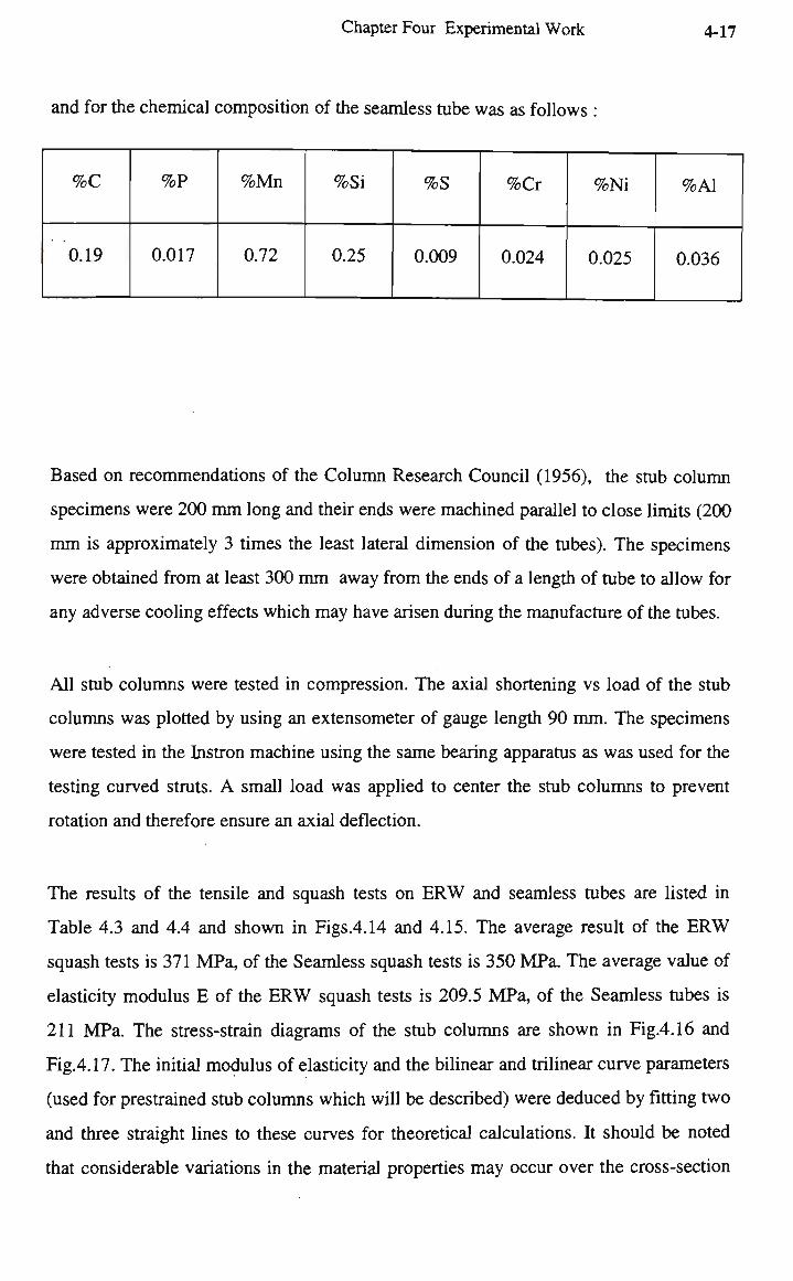
Table 4.3 Squash and Tensile Stub Column Results of E R W Tubes
Table 4.4 Squash and Tensile Stub Column Results of Seamless Tubes
Table 4.5 Concrete Cylinder Strength and Age at Test
Table 4.6 Ultimate Load Capacity of Higher Strength Concrete Infilled E R W Curved
Struts
Table 4.7 Ultimate Load Capacity of Curved Tubular Hollow Sections
Table 4.8 Ultimate Load Capacity of Higher Concrete Infilled Seamless Curved Struts
Table5.1 Ductility of Hollow and Composite Curved Electric Resistance Welded Steel
Struts
Table5.2 Ductility of Stress Relief Annealed and As Received Composite Curved Steel
Struts.
Table 6.1 Ultimate Load Capacity of E R W Composite Curved Steel Struts Obtained
From Experimental and Theoretical Results
Table 6.2 Ultimate Load Capacity of Seamless Composite Curved Steel Struts Obtained
From Experimental and Theoretical Results
Table 6.3 Ultimate Load Capacity of Curved Steel Struts Obtained From Experimental,
Finite Element and Intersection Results
Table 6.4 Reduction Coefficient for Electric Resistance Welded Composite Curved
Struts
Table 6.5 Reduction Coefficient for Seamless Composite Curved Struts
xiv
Page 17
Table 6.6 Comparison of maximum loads calculated from design formulae with loads
from experiments ( E R W Struts)
Table 6.7 Comparison of maximum loads calculated from design formulae with loads
from experiments (Seamless Struts)
Page 18
LIST of FIGURES
Fig. 1.1 The Space Trass Outside the Sydney International Airport
Fig2.1 Typical Stress-Strain Relationship for Concrete of Various Grades
Fig.2.2 Modified Kent and Park Model for Stress-Strain Behaviour of Concrete
Confined by Rectangular Steel Hoops
Fig.2.3 Details of Cross-Section and Battened Columns Used by Bridge and Roderick
(1978)
Fig.2.4 Load-Deflection Relationships for Columns CC6, CC7, C C 8 and CC10 (Bridge
and Roderick (1978))
Fig.3.1 Idealised Stress-Strain Relationship For E R W Steel Tubes
Fig.3.2 Idealised Stress-Strain Relationship For Prestrained Material
Fig.3.3 Stress-Strain Relationship of Concrete
Fig.3.4 Von Mises Criterion For A Linearly Elastic-Perfectly Plastic Material
Fig 3.5 Maximum Shear Stress Theory of Tresca Yield Criterion
Fig. 3.6 Failure Modelling of Confined Concrete Due to Local Wrinkling
Fig.3.7 Concrete Filled Circular Tube ( Stresses)
Fig. 3.8 Graphical Representation of Short Column Formulae (Oy=370 M P a and oc=60
MPa)
Fig.3.9 Flow Diagram For Load-Deflection Curve Program Assuming A n Initial
Sinusoidal Deflected Shape
Fig.3.10 Deflection of Curved Tube After Applying Load
Fig3.11 Curved Tubular Steel Section Filled With Higher Strength Concrete
Fig.3.12 Additional Deflection at Mid-Height vs Load For the Electric Resistance
Welded ( E R W ) Tube with R=2000mm and L=775mm
Fig. 3.13 Additional Deflection at Mid-Height vs Load For the Electric Resistance
Welded ( E R W ) Tube with R=2000mm and L=l 176mm
Fig.3.14 Additional Deflection vs Load For The Electric Resistance Welded Tube with
R=2000mm and L=1559 m m
Fig.3.15 Additional Deflection vs Load For The Electric Resistance Welded Tube with
R=2000mm and L=1745 m m
xvi
Page 19
Fig.3.16 Additional Deflection at Mid-Height vs Load For The Electric Resistance
Welded (ERW) Tube with R=2000mm and L=2290 m m
Fig.3.17 Additional Deflection at Mid-Height vs Load For The Electric Resistance
Welded (ERW) Tube with R=2000mm and L=3075 m m
Fig.3.18 Additional Deflection at Mid-Height vs Load For The Electric Resistance
Welded (ERW) Tube with R=4000mm and L=775 m m
Fig.3.19 Additional Deflection at Mid-Height vs Load For The Electric Resistance
Welded (ERW) Tube with R=4000mm and L=l 176 m m
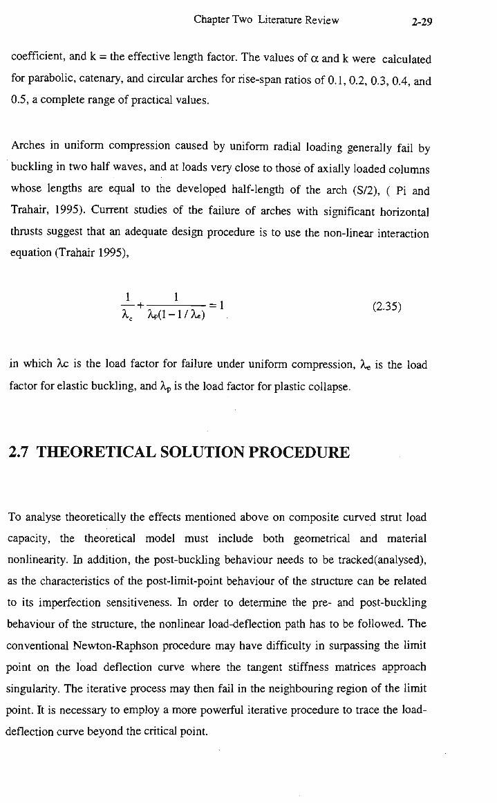
Fig.3.20 Additional Deflection at Mid-Height vs Load For The Electric Resistance
Welded (ERW) Tube with R=4000mm and L=1540 m m
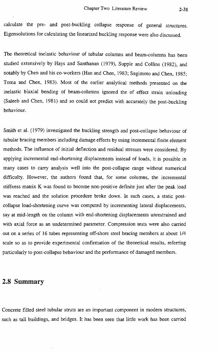
Fig.3.21 Additional Deflection at Mid-Height vs Load For The Electric Resistance
Welded (ERW) Tube with R=4000mm and L=1755 m m
Fig.3.22 Additional Deflection at Mid-Height vs Load For The Electric Resistance
Welded (ERW) Tube with R=4000mm and L=2255 m m
Fig.3.23 Additional Deflection at Mid-Height vs Load For The Electric Resistance
Welded (ERW) Tube with R=4000mm and L=3114 m m
Fig.3.24 Additional Deflection at Mid-Height vs Load For The Electric Resistance
Welded (ERW) Tube with R=10000mm and L=765 m m
Fig.3.25 Additional Deflection at Mid-Height vs Load For The Electric Resistance
Welded (ERW) Tube with R= 10000mm and L=l 141 m m
Fig.3.26 Additional Deflection at Mid-Height vs Load For The Electric Resistance
Welded (ERW) Tube with R=10000mm and L=1515 m m
Fig.3.27 Additional Deflection at Mid-Height vs Load For The Electric Resistance
Welded (ERW) Tube with R=10000mm and L=1715 m m
Fig.3.28 Additional Deflection at Mid-Height vs Load For The Electric Resistance
Welded (ERW) Tube with R= 10000mm and L=2265 m m
Fig.3.29 Additional Deflection at Mid-Height vs Load For The Electric Resistance
Welded (ERW) Tube with R=10000mm and L=3020 m m
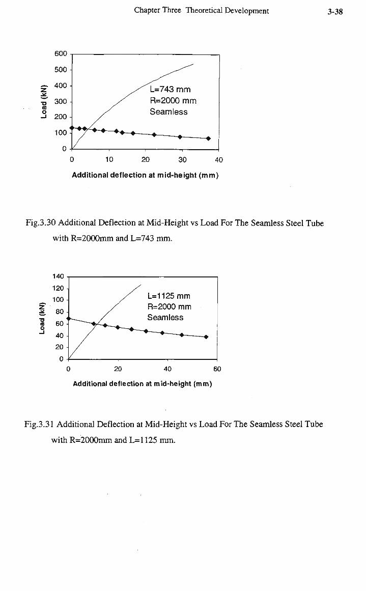
Fig.3.30 Additional Deflection at Mid-Height vs Load For The Seamless Steel Tube with
R=2000mm and L=743 m m
Fig.3.31 Additional Deflection at Mid-Height vs Load For The Seamless Steel Tube with
R=2000mm and L= 1125 m m
xvii
Page 20
Fig.3.32 Additional Deflection at Mid-Height vs Load For The Seamless Steel Tube with
R=2000mm and L=1484 m m
Fig.3.33 Additional Deflection at Mid-Height vs Load For The Seamless Steel Tube with
R=2000mm and L=1685 m m
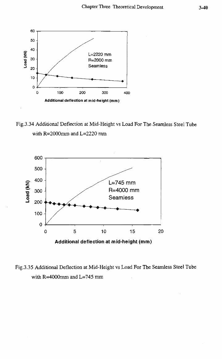
Fig.3.34 Additional Deflection at Mid-Height vs Load For The Seamless Steel Tube with
R=2000mm and L=2220 m m
Fig.3.35 Additional Deflection at Mid-Height vs Load For The Seamless Steel Tube with
R=4000mm and L=745 m m
Fig.3.36 Additional Deflection at Mid-Height vs Load For The Seamless Steel Tube with
R=4000mm and L=1120 m m
Fig.3.37 Additional Deflection at Mid-Height vs Load For The Seamless Steel Tube with
R=4000mm and L=1480 m m
Fig.3.38 Additional Deflection at Mid-Height vs Load For The Seamless Steel Tube with
R-=4000mm and L=1680 m m
Fig.3.39 Additional Deflection at Mid-Height vs Load For The Seamless Steel Tube with
R=4000mm and L=2225 m m
Fig.3.40 Nodal Displacement Vector Calculation.
Fig.3.41 Line search technique (Crisfield, 1983)
Fig.3.42 Mesh and Type of Finite Elements Used to Model The Curved Composite
Struts
Fig 3.43 Structural Characteristics of Transitional Elements Called G A P Elements
Fig.3.44 Load-Displacement Characteristic of Gap Elements
Fig.3.45. Stress-Strain Curve of the Unprestrained Stub Column and of The 1.57%
Prestrained Stub Column (Electric Resistance Welded Tube)
Fig3.46 Subdivision of Tube Section into Elementary Areas
Fig.3.47a Constraint Conditions at Support and at Mid-span
Fig.3.47b Finite Element Modelling of Half of Composite Curved Strut (half of strut is
divided into 4 segments in figure)
Fig.3.48 Deformed and Undeformed Shape of Half Composite Curved Struts and Colour
Contour plot of Bending Stresses due to Compressive Load (divided into 8
segments)(R=4000 m m and L=1515mm)
xviii
Page 21
Fig.3.49 Finite Element and Theoretical Results (elastic and plastic behaviour) of E R W
Composite Curved Strut (R=2000mm and L=775mm)
Fig.3.50 Finite Element and Theoretical Results (elastic and plastic behaviour) of E R W
Composite Curved Strut (R=2000 m m and L=l 176 m m )
Fig.3.51 Finite Element and Theoretical Results (elastic and plastic behaviour) of E R W
Composite Curved Strut (R=2000 m m and L=1559 m m )
Fig.3.52 Finite Element and Theoretical Results (elastic and plastic behaviour) of E R W
Composite Curved Strut (R=4000 m m and L=765 m m )
Fig.3.53 Finite Element and Theoretical Results (elastic and plastic behaviour) of E R W
Composite Curved Strut (R=4000 m m and L=l 176 m m )
Fig.3.54 Finite Element and Theoretical Results (elastic and plastic behaviour) of E R W
Composite Curved Strut (R=4000 m m and L=1540 m m )
Fig.3.55 Finite Element and Theoretical Results (elastic and plastic behaviour) of E R W
Composite Curved Strut (R=10000 m m and L=765 m m )
Fig.3.56 Finite Element and Theoretical Results (elastic and plastic behaviour) of
Composite Curved Strut (R=2000 m m and L=l 141 m m )
Fig.3.57 Finite Element and Theoretical Results (elastic and plastic behaviour) of
Composite Curved Strut (R=2000 m m and L=1515 m m )
Fig.3.58 Convergence of Finite Element Solution
Fig 4.1 The Length Defined for Curved Struts
Fig.4.2 The arrangement of the Rollers
Fig.4.3 Checking curvature by using scale and string
Fig.4.4 The specimen after curving
Fig.4.5 Reaction Loading Frame showing Actuator and Transducers
Fig.4.6 Instron Machine
Fig.4.7 Loading Frame for Long Specimens
Fig.4.8 Specimens After Casting Concrete
Fig4.9 Curing Specimens in the Humidity Room
Fig.4.10 Tensile Specimen
Fig.4.11 Compressive Specimen
Fig4.12 E R W Stub Column Specimen
Fig.4.13 Seamless Steel Stub column
xix
Page 22
Fig.4.14 Stress-Strain Curve for Seamless Tube
Fig.4.15 Stress-Strain Curve for E R W Tube
Fig.4.16 Compressive Stress-Strain Relationship of E R W Steel Stub Column
Fig.4.17 Compressive Stress-Strain Relationship of Seamless Steel Column
Fig.4.18 E R W Stub Column Test Prestrained 0.75 %
Fig.4.19 E R W Steel Stub Column Test Prestrained 1.5 %
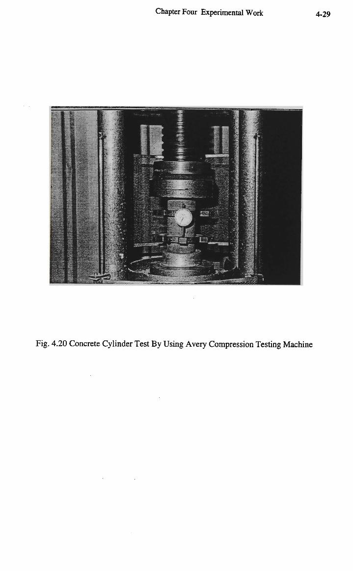
Fig. 4.20 Concrete Cylinder Test By Using Avery Compression Testing Machine
Fig.4.21 Concrete Cylinder Test By Using Instron Machine
Fig.4.22 Experimental Result for Stress-Strain Relationship of Concrete Tested by using
Instron Machine
Fig.4.23 Experimental Result for Stress-Strain Relationship of Concrete Tested by using
Avery Machine
Fig.4.24 Knife-edges Used In The Strut Tests
Fig.4.25 Deflected Shape of E R W Strut After Buckling
Fig.4.26 Deflected Shape of Seamless strut After Buckling
Fig.4.27 E R W Tubes with 2000 m m Initial Radius of Curvature
Fig.4.28 E R W Tubes with 4000 m m Initial Radius of Curvature
Fig.4.29 E R W Tubes with 10000 m m Initial Radius of Curvature
Fig.4.30 Seamless Tubes with 2000 m m Initial Radius of Curvature
Fig.4.31 Seamless Tubes with 4000 m m Initial Radius of Curvature
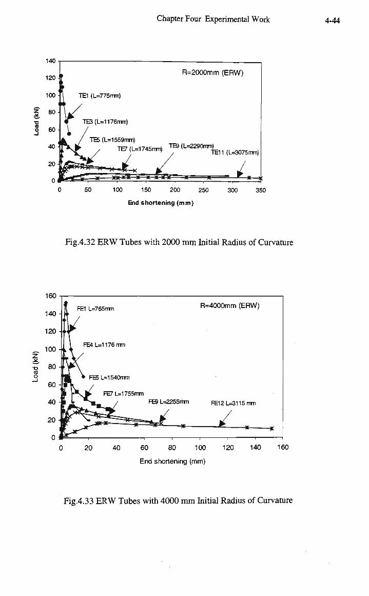
Fig.4.32 E R W Tubes with 2000 m m Initial Radius of Curvature
Fig.4.33 E R W Tubes with 4000 m m Initial Radius of Curvature
Fig.4.34 E R W Tubes with 10000 m m Initial Radius of Curvature
Fig.4.35 Seamless Tubes with 2000 m m Initial Radius of Curvature
Fig.4.36 Seamless Tubes with 4000mm Initial Radius of Curvature
Fig.4.37 Load versus end-shortening for struts T M 3 & T M 4
Fig.4.38 Load versus end-shortening for Struts T M 6 and T M 7
Fig.4.39 Load versus end-shortening for Struts T M 1 1 and T M 1 0
Fig.4.40 Load versus end-shortening for Struts F M 3 & F M 4
Fig.4.41 Load versus end-shortening for Struts F M 5 & F M 6
Fig.4.42 Load versus end-shortening for Struts F M 9 & FM11
Fig.4.43 Load versus end-shortening for Struts N E 7 & N E 8
xx
Page 23
Fig.4.44 Load versus end-shortening for Struts N E 7 & N E 8
Fig.4.45 Load versus end-shortening for Struts N E 1 0 & NE12
Fig.4.46 Load versus Lateral Deflection at Mid-height for Struts TE1 & TH1
Fig.4.47 Load versus Lateral Deflection at Mid-height for Struts TE1 & TH1
Fig.4.48 Load versus Lateral Deflection at Mid-height for Struts TE5 & T H 3
Fig.4.49 Load versus Lateral Deflection at Mid-height for Struts TE7 & T H 4
Fig.4.50 Load versus Lateral Deflection at Mid-height for Struts FE1 & FH1
Fig.4.51 Load versus Lateral Deflection at Mid-height for Struts FE3 & FE2
Fig.4.52 Load versus Lateral Deflection at Mid-height for Struts FE5 & FE3
Fig.4.53 Load versus Lateral Deflection at Mid-height for Struts FE7 & F H 4
Fig.4.54 Load versus Lateral Deflection at Mid-height for Struts NE1 & N H 1
Fig.4.55 Load versus Lateral Deflection at Mid-height for Struts N E 5 & N H 2
Fig.4.56 Load versus Lateral Deflection at Mid-height for Struts N H 1 3 & NE13
Fig.4.57 Load versus Extreme Fiber Strains at Mid-Height of E R W Tubes
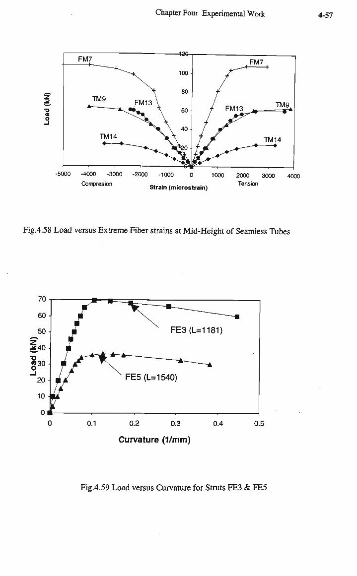
Fig.4.58 Load versus Extreme Fiber strains at Mid-Height of Seamless Tubes
Fig.4.59 Load versus Curvature for Struts FE3 & FE5
Fig.4.60 Load versus Curvature for Struts TE3 & TE7
Fig. 4.61 Load versus Curvature for Strut NE13
Fig.4.62 Load versus Curvature for Struts F M 7 & F M 1 3
Fig.4.63 Load versus Curvature for Struts T M 1 3 & T M 1 4
Fig.5.1 Shear Failure of Concrete Cylinder
Fig.5.2 Longitudinal Splitting and Local Bearing Failure
Fig. 5.3 Stress-Strain Relationship of Concrete Using different Methods
Fig.5.4 E R W Stub Column after Testing
Fig.5.5 Seamless Stub Column after Testing
Fig.5.6 Compressive Stress-Strain Relationship of E R W Steel Stub Column
Fig.5.7 Compressive Stress-Strain Relationship of Seamless Steel Column
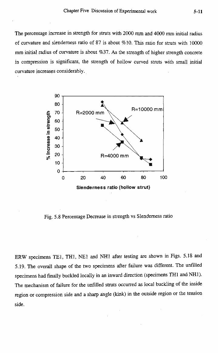
Fig 5.8 Percentage Increase in strength vs Slenderness ratio
Fig5.9a. Load-end shortening Curves of Seamless Specimens T M 6 and T M 7
Fig5.9b. Normalised Load-end shortening Curves of Seamless Specimens T M 6 and T M 7
Fig5.10a. Load-end shortening Curves of Seamless Specimens F M 3 and F M 4
xxi
Page 24
Fig5.10b. Normalised Load-end shortening Curves of Seamless Specimens F M 3 and
FM4
Fig.5.11 Load versus Curvature for E R W Struts T E 3 and T E 7
Fig.5.12 Load versus Curvature for E R W Struts FE3 and FE5
Fig.5.13 Load versus Curvature for E R W Struts FE3 and TE3
Fig.5.14 Load versus Curvature for E R W Struts N E 1 3 and FE5
Fig.5.15 Load versus Curvature for Seamless Struts T M 9 and T M 4
Fig.5.16 Normalised Load versus Curvature for Struts T M 1 4 and T E 7
Fig.5.17 Normalised Load versus Curvature for Struts F M 1 3 and FE5
Fig.5.18 Specimens TE1 & T H 1 after Testing
Fig.6.1 Load-Deflection Curves of E R W Struts (R=2000mm and L = 7 7 5 m m ) Obtained
From Experimental and Elastic and Plastic Results
Fig.6.2 Load-Deflection Curves of E R W Struts (R=2000mm and L = 1559mm) Obtained
From Experimental and Elastic and Plastic Results
Fig.6.3 Load-Deflection Curves of E R W Struts (R=2000mm and L=1745mm) Obtained
From Experimental and Elastic and Plastic Results
Fig.6.4 Load-Deflection Curves of E R W Struts (R=2000mm and L=2290mm) Obtained
From Experimental and Elastic and Plastic Results
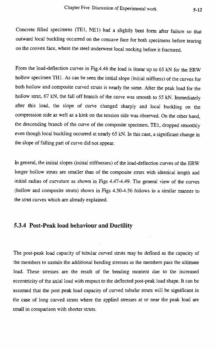
Fig.6.5 Load-Deflection Curves of E R W Struts (R=4000mm and L = 7 7 5 m m ) Obtained
From Experimental and Elastic and Plastic Results.
Fig.6.6 Load-Deflection Curves of E R W Struts (R=4000mm and L=l 176mm) Obtained
From Experimental and Elastic and Plastic Results
Fig.6.7 Load-Deflection Curves of E R W Struts (R=2000mm and L = 1540mm) Obtained
From Experimental and Elastic and Plastic Results
Fig.6.8 Load-Deflection Curves of E R W Struts (R=2000mm and L=1775mm) Obtained
From Experimental and Elastic and Plastic Results
Fig.6.9 Load-Deflection Curves of E R W Struts (R=2000mm and L=2255mm) Obtained
From Experimental and Elastic and Plastic Results
Fig.6.10 Load-Deflection Curves of Seamless Struts (R=2000mm and L = 7 4 3 m m )
Obtained From Experimental and Elastic and Plastic Results
Fig.6.11 Load-Deflection Curves of Seamless Struts (R=2000mm and L=l 125mm)
Obtained From Experimental and Elastic and Plastic Results
xxii
Page 25
Fig.6.12 Load-Deflection Curves of Seamless Struts (R=2000mm and L = 1 4 8 4 m m )
Obtained From Experimental and Elastic and Plastic Results
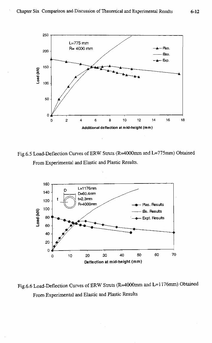
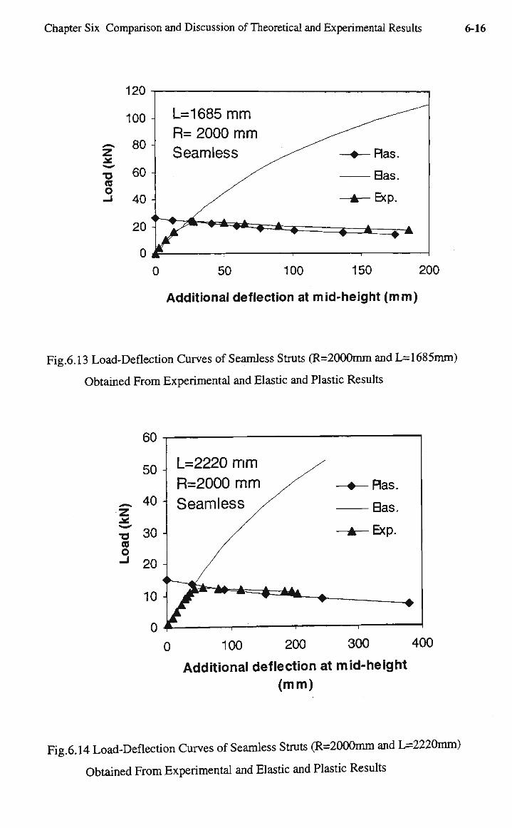
Fig.6.13 Load-Deflection Curves of Seamless Struts (R=2000mm and L = 1 6 8 5 m m )
Obtained From Experimental and Elastic and Plastic Results
Fig.6.14 Load-Deflection Curves of Seamless Struts (R=2000mm and L = 2 2 2 0 m m )
Obtained From Experimental and Elastic and Plastic Results
Fig.6.15 Load-Deflection Curves of Seamless Struts (R=4000mm and L = 7 4 5 m m )
Obtained From Experimental and Elastic and Plastic Results
Fig.6.16 Load-Deflection Curves of Seamless Struts (R=4000mm and L=l 1 2 0 m m )
Obtained From Experimental and Elastic and Plastic Results
Fig.6.17 Load-Deflection Curves of Seamless Struts (R=4000mm and L = 1 4 8 0 m m )
Obtained From Experimental and Elastic and Plastic Results
Fig.6.18 Load-Deflection Curves of Seamless Struts (R=4000mm and L = 1680mm)
Obtained From Experimental and Elastic and Plastic Results
Fig.6.19 Load-Deflection Curves of Seamless Struts (R=4000mm and L = 2 2 2 5 m m )
Obtained From Experimental and Elastic and Plastic Results
Fig.6.20 Load-Deflection Curves of E R W Struts (R=2000mm and L = 7 7 5 m m ) Obtained
From Experimental and Finite Element and Elastic and Plastic Results
Fig.6.21 Load-Deflection Curves of E R W Struts (R=2000 m m and L=1176 m m )
Obtained From Experimental and Finite Element and Elastic and Plastic Results
Fig.6.22 Load-Deflection Curves of E R W Struts (R=2000 m m and L=1559 m m )
Obtained From Experimental and Finite Element and Elastic and Plastic Results
Fig.6.23 Load-Deflection Curves of E R W Struts (R=4000 m m and L=765 m m ) Obtained
From Experimental and Finite Element and Elastic and Plastic Results
Fig.6.24 Load-Deflection Curves of E R W Struts (R=4000 m m and L=l 176 m m )
Obtained From Experimental and Finite Element and Elastic and Plastic Results
Fig.6.25 Load-Deflection Curves of E R W Struts (R=4000 m m and L=1540 m m )
Obtained From Experimental and Finite Element and Elastic and Plastic Results
Fig.6.26 Load-Deflection Curves of E R W Struts (R= 10000 m m and L=765 m m )
Obtained From Experimental and Finite Element and Elastic and Plastic Results
Fig.6.27 Load-Deflection Curves of E R W Struts (R=10000 m m and L=l 141 m m )
Obtained From Experimental and Finite Element and Elastic and Plastic Results
xxiii
Page 26
Fig.6.28 Load-Deflection Curves of E R W Struts (R=10000mm and L=1515 m m )
Obtained From Experimental and Finite Element and Elastic and Plastic Results
Fig.6.29 Reduction Coefficient vs Initial Deflection at Mid-height / External Diameter
Fig.6.30 Reduction Coefficient vs Straight Length / External Diameter
Fig.6.31 Reduction Coefficient vs Initial Deflection at Mid-height / Straight Length
Fig.6.32 Interaction Curve for COross-section Strength (O'Shea and Bridge, 1994)
Fig.6.33 Interaction Curve for Cross-section Strength
xxiv
Page 27
1. CHAPTER ONE
INTRODUCTION
1.1 INTRODUCTION
Tubular members have been widely used in roof structures, sports stadia, industrial
buildings and space structures primarily for economy and for aesthetic architectural
purposes. They have many advantages such as great torsional rigidity and offer local
strength against impact loading. However, the study and research on the structural
behaviour of curved structural members has been limited, and no design graphs have
been provided in the codes of practice for such members. Curved steel tubular members
are increasingly used in m o d e m building; for example, curved hollow tubes in space
trusses have been used at Sydney jAirport as shown in Fig. 1.1.
Tubular members are often cold formed during fabrication, and they may also be cold
formed during erection. Typical manufactured tubes are classified according to the
forming process and the heating conditions used in manufacture as follows:
1-Electric resistance welding (ERW): A strip is cold-formed by rolls into a circular
shape, and the edges are heated to welding temperature by resistance to the flow of an
electric current. This process is referred to as "cold-formed and electric resistance
welded".
2-Seamless: A heated bar is pierced one or more times, and rolled with an internal
mandrel.
Page 28
Chapter One Introduction 1-2
V \ /
g
\zs \
Ml • *'i
/-*
'*""•; J
Fig. 1.1 Space Truss of Sydney International Airport
Page 29
Chapter One Introduction 1-3
One way in which to manufacture the curved circular tubular members is by a process
that passes tubes several times through a set of rollers. A s a consequence of successive
steps in the curving process, residual stress patterns are caused by plastic deformation in
both the longitudinal and circumferential directions, in addition to the tube
manufacturing and welding residual stresses. The process of cold curving of such
members causes the steel to be strained well into the plastic range.
In the design of multi-story buildings, piles and other structures, high strength concrete
has been used because of advantages of high strength, and superior durability. Filling a
tube with high strength concrete is an attractive proposition because it considerably
increases the load-carrying capacity without increasing the size of the steel tube, and
also increases the ductility of the combination tube. Local buckling of the tube wall is
delayed because it can only buckle outwards. The hollow section provides a convenient
formwork for the concrete and an adequate cover against impact or abrasion of the
concrete surface. Finally, the concrete, in its contained condition, is able to sustain much
higher stresses and strains than when it is uncontained.
Since visual inspection of the concrete during filling the curved tube is not possible,
some difficulties such as compaction m a y be arise. Therefore, other means must be used
to check that the concrete has been properly placed and compacted.
Stability and general behaviour of straight struts and tubular composite columns have
been investigated for many years and significant theoretical achievements have been
made by many investigators such as Neogi, et, al. (1969), and Rangan and Joyce (1992).
There is a lack of information, however, about the ultimate load capacity as well as the
elasto-plastic behaviour of hollow and composite curved struts subjected to compressive
load. Prior to this investigation, some work had been carried out on the effects of the
influence of strain hardening, strain aging and the Bauschinger effect on hollow curved
steel strut load capacity (Schmidt and Mortazavi, 1993). The concrete filled curved steel
strut is a new structural element.
Page 30
Chapter One Introduction 1-4
Curved steel struts infilled with concrete subjected to compressive load herein are
treated analytically as one-dimensional stress problems. Such an analysis is suitable for
a slender metal column, a slender ordinary reinforced concrete column or a slender
encased straight composite column. In a short thin walled concrete filled steel tube,
when the lateral deformation of the concrete core is restrained by the steel shell, the core
is stressed triaxially and the tube biaxially. The stress condition in the concrete core is
similar to that in the core of a spirally reinforced concrete column. Therefore, a uniaxial
stress analysis is appropriate only in the range where triaxial stresses are non-existent or
small.
The main purpose of this study is to analyse and study the influence of initial radius of
curvature, initial deflection at mid-height, slendemess, high strength concrete, strain
hardening and residual stresses due to the forming and curving process on the ultimate
load capacity of composite curved steel struts.
1.2 SCOPE of RESEARCH
The objectives selected for this investigation are to:
(1) establish a method (numerical algorithm and its program) to calculate the
ultimate load capacity of curved composite steel tubular struts.
(2) develop a non-linear finite element analysis of the composite curved steel struts
using different material properties (stress-strain curves) across the cross section
to take into account residual stress as well as the scalar elements (Gap element)
to model the interaction of the concrete core and the steel tube.
(4) report the details of material and 78 strut tests used to study the behaviour of
curved steel struts infilled with higher strength concrete.
Page 31
Chapter One Introduction 1-5
(4) make a comparison between experimental and theoretical results and to give a
general discussion.
(5) summarise the research work conducted and draw conclusions and
recommendations for future work.
Page 32
2. CHAPTER TWO
LITERATURE REVIEW
2.1 INTRODUCTION
At the present time there is little work reported on the behaviour of slender hollow and
composite curved compression struts. Composite curved strut load capacity largely
depends on variables such as initial radius of curvature, slendemess ratio, concrete
strength, yield strength, and material type and the process of production. Composite
action between steel sections and concrete cover or core in composite columns is a
question which requires detailed analysis because of the interaction of the various
variables. It is shown that a similarity exists between the axial thrust behaviour of a
curved member subjected to compressive load and an equivalent straight column. It is
necessary to review, in addition to the information available on curved members, the
work has already been done on straight composite columns, and the properties of steel
and high performance concrete under uniaxial and multiaxial states of stress. Since the
literature in these fields, except for curved struts, is extensive, only work that is
directly relevant to this investigation will be reviewed.
Research on stability of straight struts and tubular composite columns has been carried
out for many years and significant achievements have been made in theoretical
analyses and experimental investigations. Numerical and theoretical methods have
been proposed by Neogi, Sen and Chapman (1969), Bridge and Roderick (1978),
Knowles and Park (1969), Rangan and Joyce (1992). However, there is little reported
work on the stability of curved struts, especially curved composite struts. Recently,
tubular steel arches filled with concrete were used to act as the false work to form the
reinforced concrete Joshi Bridge Arch in Japan (1993).
Page 33
Chapter Two Literature Review 2-2
2.2 GENERAL COLUMN BEHAVIOUR
It is known that the classical theories of inelastic buckling have been widely used in
the ultimate strength design of structures. A m o n g these theories, the tangent-modulus
theory is the most popular and preferred by engineers (Mansour (1986)). This is
because the tangent-modulus theory is much easier to use and gives lower critical
loads than other theories, which ensures rather safe designs.
The first correct explanation of the behaviour of a column subjected to concentrically
loaded failing by buckling in the inelastic range was given by Shanley in 1947. He
considered a simplified column model consisting of two rigid legs connected at the
center by a two flange elasto-plastic hinge. Using the Shanly approach, Duberg and
Wilder (1950) calculated the complete load-deflection curve of an idealized H-section
column with flexibility over the full length. They concluded that the tangent modulus
load is a lower bound estimate of the buckling load, and for practical purposes it may
be considered as the critical load of a concentrically loaded column.
The failure of an eccentrically loaded steel column is due to lack of equilibrium
between the internal and external bending moments. A general and exact theory for
determining the m a x i m u m load of an eccentrically loaded column was proposed by
von Karman in (1910). By assuming a different deformation behaviour regarding the
variation of strain distribution following the increase of load, Karman proposed the
reduced-modulus theory. The deflected shape of column was determined by numerical
integration of angle changes along the column length. Westergaard and Osgood
(1928) assumed the deflected shape to be part of a cosine wave and showed that this
assumption did not significantly impair the accuracy of the result. It should be noted
that a simple deflected shape with one arbitrary constant, like a part cosine wave, only
satisfies equilibrium and compatibility at the center section and at the ends.
The reduced-modulus theory has been accepted as an upper bound theory of inelastic
buckling of columns. Nevertheless, certain paradoxes do exist in both the tangent
Page 34
Chapter T w o Literature Review 2-3
modulus and reduced-modulus theories. Consequently it has been difficult to say that
there is a uniquely exact theory of inelastic buckling.
The reliability of Shanley's plastic buckling model based on the nonlinear finite
element analysis of column was investigated by Chen (1996). H e proposed an iteration
method based on improving a modified Newton-Raphson scheme for obtaining
converged solutions of discretized nonlinear algebraic systems. The continuum
modeling of the finite element method has the advantage of directly discretizing
stractural domains without imposing mechanical constraints on the stractural system.
2.3 MATERIAL PROPERTIES OF CONCRETE
In general, concrete is a heterogeneous, viscoelastic material which can carry
considerable compression but very little tension. To simplify analysis, concrete is
generally idealised as a homogenous, isotropic material having no tensile strength. In
flexural problems it is assumed that the stress-strain curve is identical with that for
uniform compression.
High performance concrete, is here defined as concrete grades above 50 MPa. The
higher strength grades offer potential for use in the lower storeys of multi-storey
buildings where the m a x i m u m axial loading occurs. High performance concretes also
offer superior durability and stiffness. In the design of tall buildings in Australia and
in other countries high performance concrete has been used not only for strength but
also for its superior stiffness (Attard, 1992).
There are several state of the art reports on high performance concretes such as the
FIP/CEB Bulletin 197 (1990), the Cement and Concrete Association publication, High
Strength Concrete (1992), and some codes of practice, such as the Norwegian N S
3473 (1989). The current Australian Standard for Concrete Structures AS3600-1988 is
only intended for concrete grades up to 50 M P a , and for normal strength concrete
Page 35
Chapter Two Literature Review 2-4
providing ties in accordance with the provisions of AS3600 provides for some
ductility (Hwee and Rangan (1989)). However, for high performance concrete, which
dilates less and requires higher confining pressures to achieve the same order of
ductility as in normal strength concrete, much larger lateral steel volumes are required.
It is well recognised that high performance concretes are much more brittle than
normal strength concretes (Attard and Mendis, 1993) (Fig.2.1). In normal strength
concrete the mortar and aggregates have higher strengths than the strength of the
resulting concrete. Failure is initiated in the weak transition zone between the
aggregate and the mortar. For high strength concrete, the mortar as well as, in most
cases, the aggregates have similar strength as the resulting concrete (Setunge et al.,
1992). Cracks at failure are reported to be smooth with little transfer of shear through
mechanical interlock.
2.3.1 Uniaxial Stress-Strain Relationship
In ultimate strength design, the stress-strain relationship and the modulus of the
concrete (Ec) are the key properties required. There are a few published papers
regarding experimental stress-strain curves for high strength concrete tested in
uniaxial compression. High strength concrete is extremely brittle and therefore
requires a very stiff testing machine with servo-control in order that the descending
branch of the stress-strain curve to be traced. The complete concrete stress-strain
compressive curve is given in CEB/FIP. In accordance with CEB-FIP ("International "
1970), the compressive stress is represented as a function of compressive strain by
oo£(a-206,600£) a = —r—T " (2-1)
l + b£
where a is in MPa, and where
a=39000(G0 + 7.0)-0'953 (2.2)
Page 36
Chapter T w o Literature Review 2-5
140
120
• 100
o | 80 i/i IA
tt
h 60
40
20
O 0-002 0 004 0-006 0008 001 0012
Strain
Fig2.1 Typical Stress-Strain Relationship for Concrete of Various Grades
Page 37
Chapter Two Literature Review 2-6
-1.085 b=65600(a0+10.0)-1U5D-85.0 (2.3)
in which ao = 0.85 fc represents the peak stress on each curve and/c is compressive
strength of concrete.
Based on limited results up to 90 MPa, the following result was proposed by Fafitis
and Shah (1986). For the ascending branch
/ = /« ( ( P Y^ 1- 1- — V
e < e, co (2.4)
where fco is the peak stress under uniaxial compression, and f is the stress
corresponding to a strain of e.
and for the descending branch
/ = fioe •k( e-e~) 1.5
e> e co (2.5)
where the strain at peak stress, eco, for gravel aggregates is
Eco — fc 3.78
Ec-VT^ (2.6)
and for crushed aggregates is f'c 4.26 ,
&» = T= , and Ectffc
A = E C s co/fco, K=2A.lfeo (2.7)
Page 38
Chapter T w o Literature Review 2-7
Experimental work to obtain the complete stress-strain behaviour of high-strength
concrete (HSC) under compression was carried out by Hsu and Hsu in 1994. They
concluded that, on average, the strain corresponding to the peak stress for the H S C is
greater than that for the normal strength concrete. Therefore, the constant values of
0.002 and 0.003 for the strain corresponding to the peak stress and the ultimate strain,
as specified by A C I Committee 318, are conservative. A s well, the crack patterns for
the H S C show that the broken surface of the concrete cylinders is smoother, and this
fracture surface passes through the aggregates.
The ascending branch of the stress-strain curve is steeper and the strain at peak load is
slightly higher for high performance concrete than for normal strength concrete. The
proportional limit occurs at a higher stress, typically 80 to 90 % of the peak stress (for
normal strength concretes the proportional limit is between 40 to 60 % of the peak
stress). The descending branch or the softening curve is almost vertical. For high
strength concrete the stress strain curve can be described as approximately linear
elastic up to the peak, and then brittle with almost complete loss of load carrying
capacity with little increase of strain (Kostovos (1983)). This implies that a triangular
stress block might be more suitable for unconfined high strength concrete in flexure.
Most published empirical formulae for the static elastic modulus of normal concrete
E c, are related to the compressive strength and the surface dry unit weight of the
concrete. The formula in AS3600 for normal strength concrete is based on the
extensive work of Pauw (1960). The AS3600 formula is quoted as
E-.---0.043p1-5 JfZ ± 20% (2.8)
where p is the surface dry unit weight, and fcm is the mean concrete strength. In most
codes, other than in Australia, the mean strength is replaced by the characteristic
strength. The in-situ strength of concrete is approximately 8 5 % of the standard
cylinder strength, and if the mean strength is approximately 1.2 times the
characteristic strength, then
Page 39
Chapter Two Literature Review 2-8
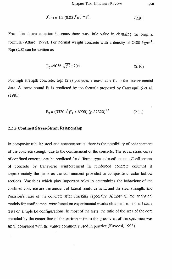
/cm = 1.2 (0.85 f c ) = fc (2.9)
From the above equation it seems there was little value in changing the original
formula (Attard, 1992). For normal weight concrete with a density of 2400 kg/m3,
Eqn (2.8) can be written as
Ec=5056 V/I±20% (2.10)
For high strength concrete, Eqn (2.8) provides a reasonable fit to the experimental
data. A lower bound fit is predicted by the formula proposed by Carrasquillo et al.
(1981),
Ec = (3320 V f'c + 6900) (p / 2320)15 (2.11)
2.3.2 Confined Stress-Strain Relationship
In composite tubular steel and concrete struts, there is the possibility of enhancement
of the concrete strength due to the confinement of the concrete. The stress strain curve
of confined concrete can be predicted for different types of confinement. Confinement
of concrete by transverse reinforcement in reinforced concrete columns is
approximately the same as the confinement provided in composite circular hollow
sections. Variables which play important roles in determining the behaviour of the
confined concrete are the amount of lateral reinforcement, and the steel strength, and
Poission's ratio of the concrete after cracking especially. Almost all the analytical
models for confinement were based on experimental results obtained from small-scale
tests on simple tie configurations. In most of the tests the ratio of the area of the core
bounded by the center line of the perimeter tie to the gross area of the specimen was
small compared with the values commonly used in practice (Kavoosi, 1993).
Page 40
Chapter Two Literature Review 2-9
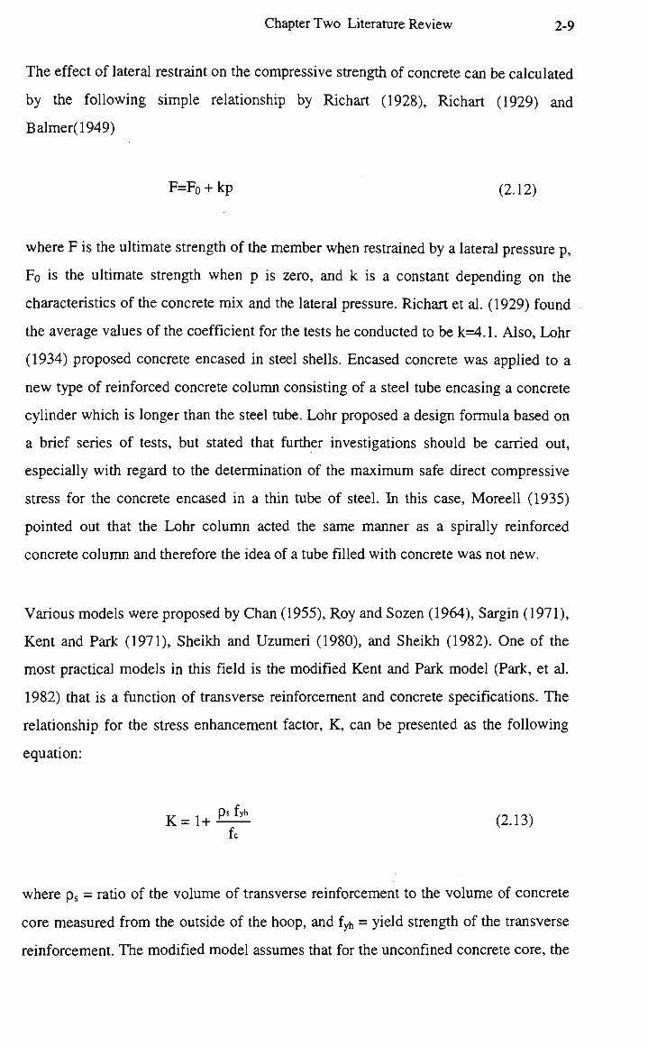
The effect of lateral restraint on the compressive strength of concrete can be calculated
by the following simple relationship by Richart (1928), Richart (1929) and
Balmer(1949)
F=F0 + kp (2.12)
where F is the ultimate strength of the member when restrained by a lateral pressure p,
F0 is the ultimate strength when p is zero, and k is a constant depending on the
characteristics of the concrete mix and the lateral pressure. Richart et al. (1929) found
the average values of the coefficient for the tests he conducted to be k=4.1. Also, Lohr
(1934) proposed concrete encased in steel shells. Encased concrete was applied to a
new type of reinforced concrete column consisting of a steel tube encasing a concrete
cylinder which is longer than the steel tube. Lohr proposed a design formula based on
a brief series of tests, but stated that further investigations should be carried out,
especially with regard to the determination of the maximum safe direct compressive
stress for the concrete encased in a thin tube of steel. In this case, Moreell (1935)
pointed out that the Lohr column acted the same manner as a spirally reinforced
concrete column and therefore the idea of a tube filled with concrete was not new.
Various models were proposed by Chan (1955), Roy and Sozen (1964), Sargin (1971),
Kent and Park (1971), Sheikh and Uzumeri (1980), and Sheikh (1982). One of the
most practical models in this field is the modified Kent and Park model (Park, et al.
1982) that is a function of transverse reinforcement and concrete specifications. The
relationship for the stress enhancement factor, K, can be presented as the following
equation:
K = l + ^ (2.13)
where ps = ratio of the volume of transverse reinforcement to the volume of concrete
core measured from the outside of the hoop, and fyh = yield strength of the transverse
reinforcement. The modified model assumes that for the unconfined concrete core, the
Page 41
Chapter Two Literature Review 2-10
maximum stress reached is Kfc, and the strain corresponding to the maximum stress is
0.002K. The detailed form of this model for the stress-strain behaviour of concrete,
according to Fig.2.2, can be shown as follows:
Range AB(ec< 0.002K)
f = Kfc 2£c f £c V
0.002K+lo.002j (2.14)
Range B C (£c > 0.002K)
f = Kfc [ 1 - Zm (£c - 0.002K)] (2.15)
but not less than 0.2KTc, in which
•Mm ~ 0.5
3 + 0.29fc
145fc-1000 4 p-iF-002K
(2-16)
and: Am — tanGn
Kf'c (2.17)
and in which fc is in MPa; K is as given in Eq. (2.13); h"= width of the concrete core
measured to the outside of the peripheral hoop; and sh = centre spacing of hoop sets.
The falling branch of the curve is suggested to be a straight line whose slope, 0m, is a
function of concrete cylinder strength, ratio of width of confined concrete to spacing
of ties, and ratio of volume of tie steel to volume of concrete core (Park et al. (1982)).
Under a triaxial stress state provided by confining pressure and the applied load, the
stress-strain behaviour of high strength concrete changes with increasing strength and
Page 42
Chapter Two Literature Review 2-11
plastic deformation due to the confining pressure (Setunge et al., 1992). It is difficult
to formulate a general theory for the deformation behaviour of confined concrete
because the uniaxial stress-strain curve is nonlinear and Poisson's ratio is a function
of the stress. Based on the extensive triaxial work on high strength concrete cylinders
by Setunge, Attard and Darvall (1992), the following equation was proposed for very
high strength confined concrete:
/ ax + bx2
fo X + cx + dx where X = —
£o (2.18)
with the peak confined stress fo and corresponding strain £o, and a,b,c and d are
constants.
t "
Rfe
Concrete stress, fc
Modified Kent and Park Confined
Kent and P*ark. Confined if K=l is assumed
0.002
Fig.2.2 Modified Kent and Park Model for Stress-Strain Behaviour of Concrete
Confined by Rectangular Steel Hoops.
Page 43
Chapter Two Literature Review 2-12
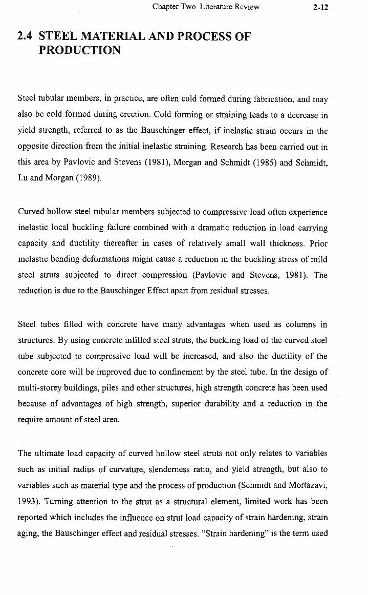
2.4 STEEL MATERIAL AND PROCESS OF PRODUCTION
Steel tubular members, in practice, are often cold formed during fabrication, and may
also be cold formed during erection. Cold forming or straining leads to a decrease in
yield strength, referred to as the Bauschinger effect, if inelastic strain occurs in the
opposite direction from the initial inelastic straining. Research has been carried out in
this area by Pavlovic and Stevens (1981), Morgan and Schmidt (1985) and Schmidt,
Lu and Morgan (1989).
Curved hollow steel tubular members subjected to compressive load often experience
inelastic local buckling failure combined with a dramatic reduction in load carrying
capacity and ductility thereafter in cases of relatively small wall thickness. Prior
inelastic bending deformations might cause a reduction in the buckling stress of mild
steel struts subjected to direct compression (Pavlovic and Stevens, 1981). The
reduction is due to the Bauschinger Effect apart from residual stresses.
Steel tubes filled with concrete have many advantages when used as columns in
structures. B y using concrete infilled steel struts, the buckling load of the curved steel
tube subjected to compressive load will be increased, and also the ductility of the
concrete core will be improved due to confinement by the steel tube. In the design of
multi-storey buildings, piles and other structures, high strength concrete has been used
because of advantages of high strength, superior durability and a reduction in the
require amount of steel area.
The ultimate load capacity of curved hollow steel struts not only relates to variables
such as initial radius of curvature, slendemess ratio, and yield strength, but also to
variables such as material type and the process of production (Schmidt and Mortazavi,
1993). Turning attention to the strut as a structural element, limited work has been
reported which includes the influence on strut load capacity of strain hardening, strain
aging, the Bauschinger effect and residual stresses. "Strain hardening" is the term used
Page 44
Chapter T w o Literature Review 2-13
to define the increase in strength with increasing strain as plastic deformation or flow
occurs beyond the yield point (Morgan and Schmidt, 1985).
"Strain aging" is the term used to describe any increase in strength or reappearance of
a discontinuous yield phenomenon occurring on reloading in the same direction of
strain as applied by the initial inelastic load. Strain aging is considered (Baird, 1963)
to be due to the migration of carbon and nitrogen atoms to dislocations causing
locking. Other changes also follow from the strain aging phenomenon. The
discontinuous yield phenomenon normally returns, the ultimate tensile strength m a y
be increased, and the elongation to fracture m a y be reduced. Baird (1963) has given an
explanation of the effects as a multistage process. The first stage is the formation of
atmospheres of carbon and nitrogen around the dislocation caused by the prestraining.
As a consequence, the yield stress increases and a reduction occurs in the elongation at
the lower yield stress. The second stage occurs when precipitates form along the
dislocations; the yield stress continues to rise, the elongation at lower yield remains
constant, but the ultimate tensile stress increases, and the elongation to fracture is
reduced.
Chajes et al.(1963) have discussed at length the effects of cold-stretching flat sheets of
steel. They showed that the effects of the cold work were directional. The Bauschinger
effect can be described in terms of three parameters: strain, stress or strain energy as
discussed by Abel et al.(1972), w h o explained that the principal causes are believed to
be associated with elastic stress and/or anisotropy in the resistance to dislocation
motion. The Bauschinger effect was observed in the longitudinal direction, together
with an inverse effect in a direction normal to the direction of straining. After an
initial inelastic tensile strain, straining in tension longitudinally causes an increase in
tensile yield strength, but causes a reduction in compressive yield strength. In the
transverse direction the opposite occurs; the compressive yield strength increases, but
the tensile yield strength decreases. Chajes et al.(1963) referred to this effect as an
"Inverse Bauschenger Effect". Such effects have been discussed also by Pascoe
(1971).
Page 45
Chapter T w o Literature Review 2-14
Bouwkamp(1975) carried out axial compressive load tests on seamless and electric-
welded steel pipes with slendemess ratios between 40 and 120. The test results agreed
reasonably well with predicted load values using the tangent-modulus expression. It
was found that local plastic buckling caused a drastic reduction of the post buckling
strength.
Chen (1977) investigated experimentally the magnitude and distribution of
longitudinal and circumferential residual stresses in fabricated steel tubular columns.
Stub column tests, and the strength and behaviour of 10 full-scale fabricated
cylindrical columns of medium slendemess ratios of 48 and 70 were investigated. It
was concluded that theoretical ultimate load analysis based on the tangent modulus
theory of an initially straight column underestimated the strength of fabricated tubular
members. Except for the shortest columns, these variations were from 8 % to 16 %. It
appeared that the transition from general plastic yielding to a local buckling type of
failure occurred at a diameter -to- thickness ratio (D/t) of about 60 for all slendemess
ratios tested.
Chan and Kitipornchai (1986) investigated the inelastic post-buckling behaviour of
beam-columns of circular hollow section. A finite element technique was employed to
study the geometric and material nonlinearities by continuously updating the geometry
of the element and by modifying the element stiffness for plasticity (the idealized
elastic perfectly plastic stress-strain model was assumed), taking into account the
influence of strain unloading. Incremental equilibrium equations were formulated in
an updated Lagrangian framework. The iterative arc-length technique (Crisfield, 1981)
was employed to trace the pre- and the post-buckling load-deflection paths. Moment-
axial-force-curvature relationships were not needed in the analysis, as only the
fundamental stress-strain relationship of the material was required. Kitipornchai et al.
(1987) modified the method proposed (Chan and Kitipornchai, 1986) and studied the
geometric and material nonlinear large deflection behaviour of structures comprising
thin-walled rectangular hollow sections. The influence of various types of residual
stress, initial geometrical imperfections, load eccentricity and yielding of material
were incorporated in the analysis. The idealized elastic perfectly plastic stress strain
Page 46
Chapter T w o Literature Review 2-15
relationship was assumed, strain hardening was neglected, but the effects of strain
unloading were included.
An extensive experimental and theoretical work was carried out to investigate the
behaviour of tensile-prestrained straight hollow-steel struts subjected to compressive
load by Lu and Schmidt (1990). They analyzed the practical influence on the hollow
steel strut load capacity of strain hardening, strain aging and the Bauschinger effect. It
was found that the influence of the Bauschinger effect was more significant on the
tubes with small initial imperfections. In the range of initial imperfections considered,
the Baushinger effect was more dominant than strain hardening and strain aging.
Considering the influence of strain aging, strain hardening and the Bauschinger effect,
the reduction in load capacities of the prestrained struts was clearly seen in
comparison with the load capacities of the corresponding as-received struts. This loss
of load capacity was due to the Baushinger effect on load reversal. Strain aging
reduced this reduction. A s well, to investigate the influence of the residual stresses set
up during the tube making process on the steel tubular strut capacity, tests on stress-
relief-annealed tubes were also performed. For the finite element modeling, three
stress-strain relationships of the steel were assumed with respect to the as-received,
prestrained in tension and fully-aged, and prestrained in tension and unaged material.
In the analysis, the cross-section of the element was divided into a finite number of
elementary areas. The structure tangent stiffness matrix was obtained by using a series
of transformation matrices to update the element geometry. Theoretical curves were
established including the effects of initial imperfections, slendemess ratios and initial
geometrical imperfections on the strut load capacities and the post-buckling
behaviour. Theoretical results were in good agreement with those obtained from
experimental results.
Page 47
Chapter T w o Literature Review 2-16
2.5 COMPOSITE COLUMNS
Serious studies on the stractural behaviour of concrete filled steel tubes began in the
decade 1950's. jAn extensive experimental investigation of the properties of concrete
filled steel tubes was carried out in Germany by Kloppel and Goder in 1954-1955.
They took into account the length of columns, whereas in previous investigations only
short members (stub columns) were considered. It was recognised that the columns
could fail by column buckling, by material failure or both. A method was prescribed
for calculating the Euler buckling load and the collapse load of the columns based on
an experimentally derived modular ratio.
Gardener and Jacobson (1967) predicted the ultimate load of short concrete filled steel
tubes and also the buckling load of long concrete filled steel tubes from an
experimentally determined load deflection curve of a stub column of similar
dimensions. They used the tangent modulus method to predict the buckling loads
which were 0 to 16.8 percent conservative. As with the long columns the composite
steel stub columns which yielded first in the longitudinal direction were tested. The
failure loads which were calculated from the sum of the failure loads of the steel and
concrete acting alone were significantly lower than the measured failure loads.
However, the combined steel stress states, and the circumferential stress in the steel,
gave good agreement with the measured failure loads. The m a x i m u m value of the
lateral restraint factor K which was used to calculate the ultimate load of short
columns appeared to be in the region of 4.1.
An experimental investigation into the stractural behaviour of concrete-filled spiral
welded steel tubes under axial load was carried out by Gardener (1968). Several spiral
welded pipe columns were made and tested to check on the applicability of
conventional design methods to this type of column. The allowable loads were
calculated using the steel properties taken from compressive tests. B y comparing the
load-strain curves for some long columns it appeared that the plain concrete stiffness
was equal to the long concrete-filled spiral welded steel tube column stiffness. This
Page 48
Chapter Two Literature Review 2-17
was illogical, and led to the conclusion that the concrete cylinders were not
representative of the concrete in the long column. This would be due to inadequate
compaction of the long columns compared with that of the cylinders. The writer
herein believes that estimating the tangent modulus for the steel from uniaxial test
results is incorrect if the steel was biaxially loaded.
The elasto-plastic behaviour of straight pin-ended, concrete-filled tubular steel
columns, loaded either concentrically or eccentrically about one axis, was studied
numerically by Neogi, Sen and Chapman (1969). They used uniaxial stress-strain
curves for steel and concrete in their analysis. In order to determine the load-deflection
curve, the differential equation governing the bent equilibrium configuration of an
eccentrically-loaded column was derived by equating internal and external forces and
moments at a displaced section. W h e n calculating external moments the deflection 8
of the section due to the applied load added to the end eccentricity. The deflected
shape was then calculated by integrating this equation along the length of the column.
To determine the complete load-deflection curve of the column, lateral deflection and
axial load values were calculated for a series of equilibrium shapes defined by
increments of curvature at the central cross-section. The peak of this curve gave the
m a x i m u m load. B y assuming the deflected shape to be part of a cosine wave the
calculation was greatly simplified. They claimed that for practical purposes the part
cosine wave deflected shape assumptions gave sufficiently accurate results for pin-
ended eccentrically loaded columns. In this case, the m a x i m u m load calculated
according to this assumption was always conservative, but not more than 5 percent
below the value given by the exact shape calculation. The concrete stress-strain curve
was represented by a single non-dimensional equation (Desayi (1964)).
Experimental investigations by Bridge (1976) have revealed that the concrete filled
steel tubes have the ability to continue to carry a substantial proportion of their
m a x i m u m loads for further deformation beyond that at m a x i m u m load. The ductility,
tenacity or toughness of the tube also prevented or delayed local buckling failure,
which would have curtailed the ductile range of behaviour.
Page 49
Chapter Two Literature Review 2-18
Ghosh (1977) carried out an experimental and theoretical study on strengthening of
slender hollow steel columns by filling with concrete. Tests were performed on long
columns under combined axial and transverse bending. The columns had a
slendemess ratio as high as 129. Ghosh concluded that concrete increased the load-
and moment-carrying capacity without increasing the size of the column. Accordingly,
thinner-walled steel columns filled with concrete could be used at considerable
savings and without loss of strength. Although the behaviour up to the ultimate load
was not established, the average of the deflection curves, assuming cracked and
uncracked concrete sections, gave sufficiently accurate results on which to predict the
behaviour of slender concrete-filled columns up to fairly high loads. However, the
tests were limited in nature, and further testing was needed to establish a revised
design standard to allow an increase in the capacity of long, slender columns due to
the contribution of the concrete fill. Pumping was found to be an effective and
economical way of filling the steel pipes and once the crews on the job became
familiar with the process, they were able to fill up to 35 pipes, 15 m high, in a single
shift with one pump.
Bridge and Roderick (1978) performed tests on encased I-section including members
made up from two or more steel components as shown in Fig.2.3. They examined the
behaviour of such members up to collapse with and without the battens. All columns
tested were of the same cross section consisting of two 3-in. (76-mm) xl-l/2in. (38-
m m ) 4.60-lb/ft (6.81-kg/m) steel channels, encased in concrete to give 2 in. (51 m m )
of cover all around. The results of all the tests are summarized in Table 2.1.
They developed a theoretical model that enabled them to take into account the full
range of linear characteristics of the material. Theoretical data were obtained from an
analysis developed as an extension of the original version by Roderick and Rogers
(1969) derived for encased rolled steel joists bent about their minor axis. The
theoretical method was based on determining the equilibrium deflected shape of a
column for successively higher values of load; the maximum load was defined as the
value at which the slope of the load deflection relationship was zero.
Page 50
Chapter Two Literature Review 2-19
Axa B»nd»a
(b)HoiorAj.li aanflPS
All Di mansions in Indus
(c) Biaxial Banding
x ER5 Gogt positioni et mid-n*-oht
0" Dial gage pu>vtioro ot ends , quarter points and mid -rvjlgni Cokjnwu
CC6.CC8
i llwt w«M
OetOrtt of bat^w DIQILH
All Omeisions In Incnas
Fig.2.3 Details of Cross-Section and Battened Columns Used by Bridge and Roderick
(1978).
Page 51
Chapter Two Literature Review 2-20
Table 2.1 Summary of Data Columns Tested by Bridge and Roderick (1978)
Column number
Type Axis of bending
Eccentricity (inches)
Maximum Load, (kips)
Observed Theoretical Observed load/
theoretical load
(a) 7-ft Composite Columns Bent About Major jAxis CC1 CC2
CC3
CC4
CC5
N o battens
N o battens
N o battens
Major
Major
Major
0 0.8 1.5
270 196 159
273 201 151
(b) 7-ft Composite Columns Bent About Other than Major.
N o battens
N o battens
- (c) CC6
CC7
End battens
4Int.batten i s
(d CC8
CC9
CC10
End battens
N o battens
Minor 49° to Major
1.5 0.8
117 158
110 150
0.99
0.98
1.05
Axis
1.06
1.05 10-ft Composite Columns Bent About Major Axis
Major
Major
0.8
0.8
21
53
20
51
1.05
1.04
10-ft Composite Columns Bent A
Major
Major
0.8
1.5
147
110
147
105 (e) 10-ft Battened Composite Column Bent About Major A
4 Int bat. Major 0.8 150 143
1.00
1.05
tis 1.05
(f) 7-ft Composite Column Bent in Double Curvature
CCIX N o battens Major 2.0 159 154 1.03
They established the load-moment-curvature relationship for the column cross section.
The residual stresses were assumed to be treated independently, and the other basic
assumptions were as follows;
Page 52
Chapter Two Literature Review 2-21
1- For the case of biaxial bending the plane of deformation was the same as the plane
of the applied end moments.
2- The complete stress-strain function for concrete was expressed in polynomial form
in which
o-c = Fc[e] (2.19)
Fc [e] = ai£ + a2£2 + a3£
3 + a4£4 for £ >£« (2.20)
Fc[£] = 0 for £<£ct (2.21)
where £« was the tensile strain at which the concrete was assumed to crack. The
constants ai, a2, &3, and an were determined from cylinder or column test results using
a method of least squares developed by Smith and Oranguan (1969).
3- The stress-strain relationship for steel was calculated from
crs = Fs [£]
Fs [£] = Es £ for -£sy<£<£sy
Fs[£]=/5y for £>£*y
Fs[£] = -/i7 for -%>£
in which £sy was the yield strain and /sy was the steel yield strength.
4- The initial imperfection c0 at the mid-height of the column in the required direction
P to the principal axes was taken as
(2.22)
(2.23)
(2.24)
(2.25)
Co = cox cos2p + Coy sin2p (2.26)
Page 53
Chapter Two Literature Review 2-22
They determined the load-deformation relationship of the column right up to the
collapse load, the collapse load and the relationship of the maximum moment
developed at collapse to the full flexural strength of the member. A typical load-
deflection of the columns is shown in Fig.2.4. They concluded that the differences in
observed and theoretical collapse loads were in the range of - 2 % and + 6 % . In such
members, the function of transmitting shear force between channels were performed
by the concrete encasement in addition to the battens. There were a range of slender
columns of the form considered, for which collapse occurred by instability before the
full flexural strength of the member was developed.
According to Rangan and Joyce (1992) the strength of eccentrically loaded straight
slender steel tubular columns filled with high-strength concrete can be calculated by
performing an analysis for the cross-section at mid-height based on assuming a sine
function for the deflection of the column. The study involved testing nine slender
composite columns under eccentric compression. The compressive strength of
concrete was 67 MPa. The eccentricity of the applied compressive load was equal at
both ends, and the columns were subjected to single curvature bending. Test
parameters were the effective length of the column and eccentricity of the applied
load. Test results are summarized in Table2.2. They assumed that the ultimate axial
load capacity Pu of a slender eccentrically loaded steel tubular column filled with
concrete was reached when the maximum moment M u was equal to the ultimate
bending moment M n at the mid-height of the column. The deflection of the column
due to creep (or long-term effects) and imperfections in the steel sheath were treated
as an additional deflection. The value of Pu was related to M „
M u = Pu (e+ Acp+Au) (2.27)
Page 54
Chapter Two Literature Review 2-23
160
140
120 -
100-
\ i
CC8 Th«or«ticol
CC8 ,CC10 " [—e = 0*8 in.
L--10ft.(3-05m)
m B o r e Steel CC6 CC71
-if— «r0-8 m. Ls10ft.(305m)
Boreo Steel- No Intermediate Bottens
Central Deflection (in.) 0-4 0-6 0-8
i 1-0 _ 1 _
Fig.2.4 Load-Deflection Relationships for Columns CC6, CC7, CC8 and CC10
(Bridge and Roderick (1978)).
Page 55
Chapter Two Literature Review 2-24
where e is the eccentricity of axial load, AcP is the creep deflection and A u is the
deflection at failure. The value of Pu, the curvature Ku, and the deflection Au at mid-
height were related by,
K U = ( T T2 / L 2 ) A U (2.28)
and £1 was the strain at the extreme compressive fiber (Fig.2.4) given by,
ei = 0.003 dn / (dn -1) (2.29)
where t was the wall thickness of the steel tube. The curvature also was given by,
Ku = £i / dn (2.30)
K„ = 0.003 / (dn-t) (2.31)
in which d„ is the depth of neutral axis. It was assumed that the tubular steel section
was split into two strips about the neutral axis. The area of concrete in the
compression zone was assumed to be lumped at its centroid. Similarly, the area of
steel in the tension zone and in the compression zone were concentrated at their
respective centroids.
Page 56
Chapter Two Literature Review 2-25
ul
Fig.2.5 Curved Tubular Steel Section Filled With Higher Strength Concrete
Table 2.2 Summary of Data Columns Tested By Rangan and Joyce
Specimen No.
1 2 3 4 5 6 7 8 9
Effective length L,mm
807.5
807.5
1312.5
1312.5
1565.0
1817.5
1817.5
2322.5
2322.5
Eccentricity e, m m
10 30 10 30 10 10 30 10 30
Deflection at mid-
height, m m
-
2.91
6.69
9.38
11.54
13.56
12.00
18.69
15.73
Failure load P„,kN
Test
430 235 350 190 315 280 140 220 126
Calculated
376 219 332 182 303 266 129 155 79
Test/Calculated
1.14
1.07
1.05
1.05
1.04
1.05
1.08
1.42
1.6
Rangan and Joyce used the following equations to estimate the strength of slender
composite columns,
Page 57
Chapter Two Literature Review 2-26
PU=CC+CS-T (2.32)
Mn= (Cszsc+Tzst+Cczc) (2.33)
in which Cs= Ascasc ; T=AstO"st; Cc =Acac; and zsc, zst, and zc were the lever arms
of forces from the plastic centroid (Fig.2.5). The steel stresses were o s c = Es£idsc/dn
and ost= Es£idst/dn. W h e n the steel stresses were larger than the yield stress, they
were taken as fsy. E s was the modulus of elasticity of the steel, and dsc and dst were
the distances of the respective centroids of the steel areas from the neutral axis.
The calculation procedure of the strength of eccentrically loaded straight and slender
steel tubular column filled with high-strength concrete is briefly explained below;
1-Select a suitable value for the depth of neutral axis dn. For this value of dn, calculate
Ei by Eq. (2.29), and calculate all stresses.
2- For these values, calculate Pn and Mn by Eqs. (2.32), (2.33). Also, calculate Ku and
Au by Eqs. (2.31) and (2.28).
3- Calculate j^p and estimate deflections due to initial imperfections in the steel
sheath when they are significant and add these to AcP.
4. For these values of Au and AcP, take Pu = Pn and calculate Mu by Eq. (2.27). The
selected value of d„ is accepted when M u = M „ and strength of the column is pu.
Rangan and Joyce found that there was good correlation between tested and calculated
results as well as with those available in the literature. The mean value of
test/calculated for 27 columns (including literature data) was 1.17, with a coefficient
Page 58
Chapter Two Literature Review 2-27
of variation of 16 percent. The calculated strengths were very conservative for
columns with small eccentricity (e/D=0.05), perhaps due to the assumption that
£u=0.003 at failure for the concrete.
Shakir-Khalil (1993) reported tests on pushout strength of concrete-filled steel hollow
sections. The tests showed clearly that the resistance of the specimens to the pushout
load was a function of the shape and size of the steel hollow section used, and also the
condition of the steel-concrete interface. H e mentioned that for the tested specimens
with an oiled steel-concrete interface, resulted in halving the bond resistance of the
concrete-filled steel hollow sections. The test results clearly showed how sensitive the
bond strength was to the interface conditions. H e used steel-concrete interface lengths
of approximately 200, 400 and 6 0 0 m m , i.e. in the ratio of 1:2:3. The failure loads of
each group of the specimens, dry or oiled, were not in a similar ratio. The average
bond strength result for each group indicated that the bond strength of circular
specimens was on average about 82 % and 64 % higher than that of the rectangular
specimens for the 'dry' and 'oiled' conditions, respectively. The 'dry' specimens gave
an average bond strength that were about twice those of the 'oiled' specimens for both
the rectangular and circular specimens. In general, Shakir-Khalil concluded that the
bond strength, as based on the pushout failure load, was rather sensitive to the local
imperfections of the steel-concrete interface and also to the overall longitudinal
variations in the dimensions of the steel hollow sections.
Kavoossi and Schmidt (1993) carried out an experimental and theoretical study on the
behaviour of confined higher strength concrete (HSC) in steel circular hollow sections
with emphasis on the dependence of the radial stress on the axial stress in the confined
concrete. The results of the study showed that the brittle behaviour of higher strength
concrete could be modified considerably by confining the concrete in a steel tube.
They concluded that the apparent elastic parameters, such as the modulus of elasticity
and Poisson's ratio in a hollow steel tube under axial compression depended on the
dimensions of the specimen. In the tests of confined concrete, the concrete mass was
loaded, and the steel tube yielded longitudinally. This effect showed that the axial
load, in a very short length, transferred load to the steel tube. The increase of the
Page 59
Chapter T w o Literature Review 2-28
compressive strength of the confined concrete in a steel tube was in fair agreement
with the proposed equation by Cai (1986). The ductility factor, the ratio of load at any
specific strain over the ultimate axial load, showed that the concrete encased in thick
walled tubes was more ductile than the concrete in thin walled tubes.
2.6 CURVED MEMBERS AND ARCHES
As mentioned in the previous section the ultimate load capacity of concrete infilled
curved steel struts largely depends on variables such as initial curvature, slendemess
ratio, concrete strength, yield strength of steel, and the effect of confining pressure on
the compressive strength of the concrete. Imperfections of shape of the member are of
lesser importance than for the case of straight struts due to the dominant initial
curvature.
In general, arches support their loads by a combination of axial compression and
bending actions, except in the case of uniform radial loading, which is resisted by
uniform axial compression alone. Thus their in-plane behaviour varies from the
buckling failure of members under end axial compression to the plastic collapse of
flexural members. The relative importance of the compression and bending actions
depends on the arch loading, and on its rise/span ratio.
Elastic buckling of arches under loadings which produce pure axial compression was
investigated by Walter and Austin (1971). They computed the critical axial thrust in
an arch conveniently by the following equation which is identical in form to that used
for straight compression members,
Pe=ccEI / S2 = TT2 EI / (kS)2 (2.34)
in which Pe = the critical axial compressive force; E = Young's modulus; I = second
moment of area of the cross section; S = one-half the length of the arch axis; a = a
Page 60
Chapter Two Literature Review 2-29
coefficient, and k = the effective length factor. The values of a and k were calculated
for parabolic, catenary, and circular arches for rise-span ratios of 0.1, 0.2, 0.3, 0.4, and
0.5, a complete range of practical values.
/\rches in uniform compression caused by uniform radial loading generally fail by
buckling in two half waves, and at loads very close to those of axially loaded columns
whose lengths are equal to the developed half-length of the arch (S/2), ( Pi and
Trahair, 1995). Current studies of the failure of arches with significant horizontal
thrusts suggest that an adequate design procedure is to use the non-linear interaction
equation (Trahair 1995),
in which A,c is the load factor for failure under uniform compression, A*, is the load
factor for elastic buckling, and Xp is the load factor for plastic collapse.
2.7 THEORETICAL SOLUTION PROCEDURE
To analyse theoretically the effects mentioned above on composite curved strut load
capacity, the theoretical model must include both geometrical and material
nonlinearity. In addition, the post-buckling behaviour needs to be tracked(analysed),
as the characteristics of the post-limit-point behaviour of the structure can be related
to its imperfection sensitiveness. In order to determine the pre- and post-buckling
behaviour of the structure, the nonlinear load-deflection path has to be followed. The
conventional Newton-Raphson procedure may have difficulty in surpassing the limit
point on the load deflection curve where the tangent stiffness matrices approach
singularity. The iterative process may then fail in the neighbouring region of the limit
point. It is necessary to employ a more powerful iterative procedure to trace the load-
deflection curve beyond the critical point.
Page 61
Chapter T w o Literature Review 2-30
The arc-length method technique has been independently introduced by Riks (1972
and 1979) and W e m p n e r (1971). Both authors limit the load step by a constraint
equation; that is, the generalized "arc length" of the tangent at a converged point of
the load-displacement curve is fixed to a prescribed value. Then the iteration path
follows a "plane" normal to the tangent path. The Newton-Raphson method is not
often used with the finite element method, the modified Newton-Raphson method
(m.N-R) being generally preferred (Zienkiewicz, 1977). W h e n using the m.N-R
procedure, the tangent stiffness matrix is neither re-formed nor re-factorized at each
iteration but is, instead, held fixed. Even having substituted the m.N-R method for the
N-R method for the N-R procedure, Riks'technique is still not suitable for use with the
standard finite element method, because the direct simultaneous solution of the
relevant equations destroys the symmetric banded nature of the equilibrium equations
on their o w n (with a loading parameter X taken as a constant). The technique has been
modified by Crisfield(1981) and Ramm(1981), so that it is suitable for use with the
finite element method. In addition to the "constant-arc-length", the step size may be
scaled by relating the number of iterations used in the previous step to a desired value.
If material nonlinearities are involved smaller load steps should be defined to avoid
drifting. Whenever a negative element in the triangularized stiffness matrix is
encountered unloading is initiated.
Bergan et al. (1978) use the "current stiffness parameter" , to predict the local
m a x i m u m or minimum. They then suppress the equilibrium iterations in the
neighbourhood of the extreme (limit) point and reverse the sign of the load following
a change in the sign of the determinant of the tangent stiffness matrix. The
suppression of the equilibrium iterations dictates the provision of very small load
increments close to the limit point and also leads to a local drift from equilibrium.
Bathe et al. (1983) presented an algorithm for the automatic incremental solution of
nonlinear element equations in static analysis. The procedure used two different
constraints depending on the response and load level considered; i.e., the spherical
constant arc-length and a constant increment of external work. It was designed to
Page 62
Chapter Two Literature Review 2-31
calculate the pre- and post-buckling collapse response of general stractures.
Eigensolutions for calculating the linearized buckling response were also discussed.
The theoretical inelastic behaviour of tubular columns and beam-columns has been
studied extensively by Hays and Santhanan (1979), Supple and Collins (1982), and
notably by Chen and his co-workers (Han and Chen, 1983; Sugimoto and Chen, 1985;
T o m a and Chen, 1983). Most of the earlier analytical methods presented on the
inelastic biaxial bending of beam-columns ignored the of effect strain unloading
(Saleeb and Chen, 1981) and so could not predict with accurately the post-buckling
behaviour.
Smith et al. (1979) investigated the buckling strength and post-collapse behaviour of
tubular bracing members including damage effects by using incremental finite element
methods. The influence of initial deflection and residual stresses were considered. By
applying incremental end-shortening displacements instead of loads, it is possible in
many cases to carry analysis well into the post-collapse range without numerical
difficulty. However, the authors found that, for some columns, the incremental
stiffness matrix K was found to become non-positive definite just after the peak load
was reached and the solution procedure broke down. In such cases, a static post-
collapse load-shortening curve was computed by incrementing lateral displacements,
say at mid-length on the column with end-shortening displacements unrestrained and
with axial force as an undetermined parameter. Compression tests were also carried
out on a series of 16 tubes representing off-shore steel bracing members at about 1/4
scale so as to provide experimental confirmation of the theoretical results, referring
particularly to post-collapse behaviour and the performance of damaged members.
2.8 Summary
Concrete filled steel tubular struts are an important component in modem stractures,
such as tall buildings, and bridges. It has been seen that little work has been carried
Page 63
Chapter T w o Literature Review 2-32
out on the stability and ultimate load capacity of such stractures subjected to an
eccentric load. Various methods such as using exact and a cosine wave for deflected
shape (Neogi, 1967), determining the equilibrium deflected shape for successively
higher values of load (Bridge, 1978) and using an iteration process (Rangan, 1992)
have been used to calculate ultimate load capacity of slender columns filled with
concrete subjected to eccentric load.
Page 64
3. CHAPTER THREE
THEORETICAL DEVELOPMENT
3.1 GENERAL
The aim of this study is primarily to present a simple theoretical and computational
method based on assumptions which will enable to be estimated the ultimate load
capacity of curved composite struts. A s well, in order to predict the load-deformation
behaviour of curved composite steel strut elements over the entire elastic-plastic range
the finite element method will be used. The effects of all parameters which significantly
influence load-deformation will be taken into account.
Such theoretical procedures were required to make a full comparison with the
experimental results which will be described in Chapter four. The calculation
procedures were programmed in a computer whenever needed. Iterative methods were
employed to determine the ultimate load capacity of the curved struts. A finite element
program (Nastran) enabled material and geometric nonlinearity to be taken into account
to predict the detailed load-deflection behaviour.
3.1.1 Basic Assumptions
The following basic assumptions have been made:
1. Plane sections before deformation remain plane after deformation.
Page 65
Chapter Three Theoretical Development 3-2
2. Complete interaction takes place between the tube and the core, i.e. there is no
longitudinal or circumferential slip.
3. Failure due to local buckling of the steel tube does not occur.
4. Concrete cannot carry tensile stress.
5. The concrete stress-strain curve is identical in pure compression and flexure.
6. Yielding is governed by direct stress only. Shear strains due to bending are not
considered.
7. Strains are small but displacements and rotations can be arbitrarily large.
These simplifying assumptions are made by most workers in the field of reinforced
concrete and composite columns.
3.1.2 Uniaxial Stress-Strain Curve for Steel
It is essential to obtain the stress-strain relationship for the modeling used in any
structural analysis. Based on the observation of material behaviour, the stress-strain
relationship of the electric resistance welded ( E R W ) steel stub column is approximated
by a bilinear curve upon loading, as shown in Fig.3.1. To take into account the effect of
curving and residual stress, the stress-strain relationship of the prestrained stub column
is approximated by a fourth curve, as shown in Fig.3.2. Stress, o\ may be related to
strain, £, by following equations:
1. ERW tube material (see Fig.3.1)
ai = Es£i for .£il<l£yl (3.1)
= rjy + (£i-£y)Es (loading) for I ej >l£yl (3.2)
= E (£j - £pi) (unloading) (3.3)
Page 66
Chapter Three Theoretical Development 3-3
£pi = £raax-(ey + (£max-£y))Es/E (3.4)
2. Prestrained material (see Fig.3.2)
c>i = E£i for IEII <|EJ (3.5)
= CTS + (£i-£s)Et for l£sl<UI >Uyl (3.6)
= cyx + (£r£x)Ex for l£xl<Uil >l£yl (3.7)
= ay + (£i-£y)Es (loading) for |£SI<|E| >| £y (3.8)
= (£i-£pi)E (unloading) (3.9)
£pi = £max " (£sn + ( £max - £y ) Es / E (3.10)
where £s„ = ciy / E (3.11)
The incremental stress-train relationship can be found by a variation of the above
equations. In the elastic range ( I £i I < I £y I or I $ I < I £s I) and on the unloading and
reloading paths (I d I < I ay I and I £i I < I £s I), and dd = E 5£i.
In the inelastic range I £j I > I £* I), 5oj = Et &* or 5di = Ex &i or 5oi = Es 8£j, depending
on the inelastic model used.
3.1.3 Uniaxial Stress-Strain Curve for Concrete
The complete concrete stress-strain curve is obtained by using the CEB-FIP
("International" 1970) model as shown in Fig.3.3. In accordance with the "International
" (1970) model, the compressive stress is represented as a function of compressive strain
by
Page 67
Chapter Three Theoretical Development 3-4
Fig.3.1 Idealised Stress-Strain Relationship For E R W Steel Tubes
4
Page 68
Chapter Three Theoretical Development 3-5
Fig.3.2 Idealised Stress-Strain Relationship For Prestrained Material
Page 69
Chapter Three Theoretical Development 3-6
50-
40-
20-
0.0005 0.001 0.0015 0.002 0.0025 0.003 0.0035
Strain
Fig.3.3 Stress-Strain Relationship of Concrete
Page 70
Chapter Three Theoretical Development 3-7
co£(a-206,600£)
° = — — r - z ~ 0.12) 1 + be
where a is in M P a , and where
r0.953 a=39000(a0 + 7.0)"™ (3.13)
-1.085 b=65600(a0 + 10.0) "lu"-85.0 (3.14)
in which ao = 0.85 fc represents the peak stress on each curve.
3.1.4 Biaxial Yield Criterion for Steel
As the steel tube is stressed biaxially, it is necessary to assume a biaxial yield criterion
for the steel. The von Mises criterion has been used in this study (Fig. 3.4); it should be
noted that all this criterion refers to the first yield of a linear elastic material. In the
inelastic range, the failure envelope can remain identical with the first yield envelope
only if the material does not strain harden, i.e. if it has a linearly elastic-perfectly plastic
uniaxial stress-strain curve.
The yield criterion of Von-Mises represents an ellipse in the biaxial plane. The principal
stresses at first yield are therefore related by the equation
CJn +CT22 -CTu a22 = C7y (3.15)
where O n and 022 are maximum and minimum principal stresses, respectively.
Page 71
Chapter Three Theoretical Development 3-8
W h e n considering the difference in compression and tension yield capacity of a
material, a modified Von-Mises criterion is also suggested in the following equation
(Raghava,1973)
(Oi i-c22)2+(a22-cJ33)
2+(a33-cri i)2+2(C-T)(oi i+a22-KJ33)=2CT (3.16)
where, T,C are yield strength in uniaxial tension and compression respectively, and On,
G22 and O33 are principal stresses in a three dimensional principal stress space.
According to Raghava this criterion was originally proposed by Schleicher in 1926, and
was suggested independently by Stassi-D'Alia in 1967. The von-Mises yield criterion
was also modified for anisotropic behaviour of materials by Theocaries (1989).
In addition to the Von-Mises yield criterion, the Tresca yield criterion of maximum
shear theory assumes that yield will occur when the maximum shear stress reaches the
value of m a x i m u m shear stress occurring under simple tension. The maximum shear
stress is equal to half the difference between the maximum and minimum principal
stresses. Therefore, since 0i 1=022=0, under simple tension the m a x i m u m shear stress at
yield is CTn/2. Accordingly, yield will occur when any one of six following conditions is
reached:
0n-022=±0y (3.17)
0"22-C33=±CTy (3-18)
0"33-Oll=±CTy (3-19)
These equations represent a cylindrical shape with a hexagonal cross-section, along the
normal axis to the 7C-plane (011+022+033 =0) from the center of coordinates in a
"011,022,033" coordinate system. The cross-section of this cylinder with the plane of
(011-022) is shown in Fig. 3.5.
Page 72
Chapter Three Theoretical Development 3-9
Fig.3.4 V o n Mises Criterion For A Linearly Elastic-Perfectly Plastic Material
Fig 3.5 M a x i m u m Shear Stress Theory of Tresca Yield Criterion
Page 73
Chapter Three Theoretical Development 3-10
3.2 TRIAXIAL ANALYSIS of CONCENTRICALLY
LOADED STUB COLUMNS
3.2.1 General Behaviour
W h e n the steel and the concrete of the composite column are subjected to the
compressive load in the early stage of loading the Poisson's ratio for concrete is smaller
than that for steel. The steel expands more than the concrete and the steel tube has no
restraining effect on the concrete core. These two materials would separate unless the
cohesion between the steel and the concrete was sufficient to maintain contact. This
cohesion exerts an inward radial pressure on the tube, therefore producing a small hoop
compressive stress in the steel.
As the longitudinal strain increases, an outward radial pressure develops at the steel
concrete interface due to expanding and cracking concrete inside the tube, thereby
setting up a hoop tension in the tube as shown in Fig.3.6. A s long as the steel remains
elastic, the stresses can be determined from the strains. A s the load is further increased
the steel tube yields in longitudinal compression, and both longitudinal and lateral
strains continue to increase. W h e n the column fails the hoop strain in the tube is also in
excess of the uniaxial yield strains.
Failure may be initiated by a local wrinkling of the tube as shown in Fig.3.7. It is
difficult to establish criteria for the occurrence of this phenomenon. If this possible
failure mode is excluded, simple relations can be established for the failure load of a
stocky column regarding the behaviour of the steel tube and the concrete core.
Page 74
Chapter Three Theoretical Development 3-11
OSH 0SH
OCR
OSL
i OSH
Fig.3.6 Concrete Filled Circular Tube ( Stresses)
3.2.2 Failure Load Corresponding to The Hoop and Longitudinal
Failure Mode of Concentrically Loaded Stub Column
The following equations were suggested by Richart (1928), Lohr (1934), Moreel (1935)
and Neogi (1967) to calculate the longitudinal stress and radial stress in the concrete
core at the ultimate stage of loading:
0 C L = f'c + K. 0CR (3.20)
where f c = unconfined compressive strength of concrete, K = an empirical factor, and
0 C R = radial stress on concrete (Fig.3.6). For a thin-walled tube the hoop stress 0 S H may
be assumed to be constant over the wall thickness (Fig. 3.6). Considering the
equilibrium of a semi-circular half of the steel shell,
Page 75
Chapter Three Theoretical Development 3-12
2t C?CR ~ 0"SH • —
di (3.21)
where t is the wall thickness of the tube and di is the internal diameter for circular tube.
Eq.3.20 can be expressed as:
2t O"CL = f c + K. asH • —
di
(3.22)
The total load carried by the concrete filled tube is
P = A C aCL + A s a y
2t A c ( f c + K. a S H — ) + As aSL
di
(3.23)
(3.24)
Fig. 3.7 Failure Modelling of Confined Concrete Due to Local Buckling
Page 76
Chapter Three Theoretical Development 3-13
The failure loads can be calculated from
2t PH = A c ( f c + K . 0 y — ) (3.25)
di
PL = Ac f c + As 0SL (3.26)
where PH is the ultimate load corresponding to the hoop failure mode and PL is the
ultimate load corresponding to the longitudinal failure mode. The load P L is the same as
the squash load of an ordinary reinforced concrete or composite column. For a thin
walled tube,
2t As
di ~ 2Ac
Substituting this relation in Eq.3.25, and assuming K=4 (Neogi, 1967), this equation
may be rewritten as
PH = Ac f c+ 2 As 0y (3.27)
which indicates that at failure, the steel is twice as effective in hoop tension as
longitudinal compression. The variation of strength with wall thickness is shown in
Fig.3.8 for a particular tube, assuming K=4. For a practical tube size i.e. 8 < d/t > 50 ,
the hoop failure load is always greater than the longitudinal failure load (Neogi, 1967).
Page 77
Chapter Three Theoretical Development 3-14
1200
1000
800-
600-Load (kN)
400
200 -I
0
d=60.4 m m rc=60 MPa Oy =340 MPa
10 20 30 40 50 60
External diameter/wall thickness (m/m) 70
Fig. 3.8 Graphical Representation of Short Column Formulae (0y=37O M P a and 0C=6O
MP a ) .
The ultimate strength of circular hollow sections filled with concrete has been
conveniently described by different codes of practice. But the generity of the
recommended equations to include the wide range of material properties for steel tubes
and concrete furnish considerable differences between the computed strength of
composite columns with the actual strengths.
The mechanical behaviour of higher strength concrete is entirely different with the
ordinary strength concrete. The higher strength concrete is more brittle than ordinary
concrete. Restrictions for use of higher strength concrete in the filled circular hollow
sections has not been specified as accurately as recommended in specifications for
reinforced concrete. In the case of thin walled tubes, the brittle behaviour of the higher
strength concrete and the formation of major cracks in the concrete mass cannot be
prevented by the steel tube. This behaviour of circular hollow sections filled with higher
strength concrete leads to unpredictable behaviour, and in some cases it may cause
brittle failure in the structural member.
Page 78
Chapter Three Theoretical Development 3-15
A n experimental research program was carried out on the prediction of ultimate load
capacity of C H S filled with higher strength concrete and the structural behaviour of
these elements in elastic and plastic stages of loading by Kavoossi and Schmidt (1993).
To achieve the most realistic model of these columns, they used two methods of
loading: load on both steel tube and the concrete core, and load on steel tube only. They
suggested the following equation for computing the ultimate load capacity of short
circular hollow sections filled with concrete:
Pu = 0.9AS fy + Ac [ 1.065 f c + 2.148(t/2)fy] (3.28)
where As is steel cross section area, Ac is concrete cross section area, t is wall thickness,
fy is steel yield strength, and f c is concrete cylinder strength.
3.3 UNIAXIAL TANGENT MODULUS ANALYSIS of
CONCENTRICALLY LOADED PIN ENDED
COMPOSITE COLUMNS
The first theory for the maximum load of an axially loaded elastic pin ended column
was obtained by L. Euler in 1757. The failure load P E is given by
PE=^ (3-29)
where PE is known as the Euler load, EI flextural rigidity, and L is length of pin ended
column. Euler recognised that this equation applied only to long slender columns in
which the material remains linearly elastic. Euler's theory was verified by a series of
experiments carried out by von Karman and others about 1900.
Page 79
Chapter Three Theoretical Development 3-16
The tangent modulus buckling load P T M is that value of the load P which simultaneously
satisfies the equations
K2 P T M - p' = —tr ( ETs Is + ETc Ic
l2 (3.30)
and
P T M = P" = A s a S L + Ac a C L (3.31)
where ETC is the tangent modulus of concrete, ETs is the tangent modulus of steel, 1 is
effective length of the column, A c is the concrete cross-section area, A s is the steel
cross-section area, Ic and Is are second moments of areas of the concrete and the steel
respectively. The above equations can be solved by a graphical method. These formulas
can be adapted to allow for various conditions of fixity at the ends of the columns by
replacing 1 by the effective length K L where K is a constant depending on the degree of
fixity.
3.3.1 Stress-Strain Relationship
W h e n the tube has a thin wall it is assumed that the steel is subjected only to two normal
stresses. The radial stress acting on the element is small and is neglected; the
circumferential stress is assumed to be constant over the thickness. As long as the steel
is in the linear elastic range, the steel and concrete stresses can be calculated from the
steel strains, using the following equations
Es CTSL = ( £SL + vs eSH) (3.32)
1-Vs
Page 80
Chapter Three Theoretical Development 3-17
O S H = ( £SH + vs eSL) (3.33) 1 — Vs
Pc = P"PS
0CL:
OCR
P-As
Pc
" Ac
= OSH-
•0SL
2t
di
(3.34)
(3.35)
(3.36)
(3.37)
where Pc is the axial load carried by the concrete core, Ps is the axial load carried by the
steel tube, £SL and 8SH are longitudinal and hoop strains, 0 S L and 0 S H are longitudinal
and hoop stresses in the steel, 0 C L and 0 C R are longitudinal and radial stresses in the
concrete, respectively. As it is also assumed that there is no longitudinal or
circumferential slip between the steel and concrete,
£SL = £CL and £SH = £CR
If the concrete is assumed to behave like a linear elastic material in the range, the
concrete strains are given by the following equations:
£CL = — • ( O C L - vc 0 C R ) (3.38) Ec
£CR = — • ( OCR - Vc ( 0 C L + OCR ) (3.39) Ec
where Ec and vc are the initial concrete modulus and Poisson's ratio respectively; both
are assumed to remain constant in this range.
Page 81
Chapter Three Theoretical Development 3-18
3.4 ULTIMATE STRENGTH of COMPOSITE CURVED
STRUTS
The failure load of a curved strut is the item of prime interest to the designer, but
unfortunately there is no easy means of obtaining it. At failure there is a complex
interaction for the cross section behaviour such as the spread of plasticity, position of
neutral axis as well as the deflected form of the strut. One of the methods, that may be
employed, is an iteration process.
An iteration process was used to determine the strength of the curved composite tubes.
The ultimate load capacity was calculated from the intersection point of inelastic and
elastic behaviour, which will be described later. The calculation procedure was
programmed in a computer by using Fortran 77. The flow diagram is shown in Fig.3.9.
3.4.1 Elastic Behaviour
To avoid more complex analysis it was assumed that there was an initial sinusoidal
deflected shape. M a x i m u m strength of the members subjected to compressive load
largely depends on the slendemess of the members. Based on Bar-Spring model of a
axially loaded column (Warner et al., 1989) the end thrusts (Pu2 is shown in Fig.3.10) in
a curved strut can be related to the initial deflection (e) and additional deflection (Au ) at
mid-height (see Fig.3.10) as
e+Au = e (3.40) . u 1-Pu2/Pcri.
Pu2 = AuPcrit/(e + Au) (3.41)
Page 82
Chapter Three Theoretical Development 3-19
where Pcrjt is the elastic critical load for a pin-ended stmt, that is, the Euler load
7t2EI/L2. Here L is assumed to be the straight length for convenience, and EI the
effective flextural rigidity, according to A C I (1977), is taken as,
EI=l/5EcIg + EsIs (3.42)
where lg is the second moment of the gross cross-section area and Is is the second
moment of steel cross-section area.
3.4.2 Inelastic Behaviour
The cross section strength, at mid-height, Pui, was calculated as shown in Fig.3.11. The
tubular steel section was divided into two strips about the neutral axis. The area of steel
in the compression zone is denoted by Asc, and the area of tension by Ast. Similarly, the
area of concrete in compression is Ac. It was assumed that the area of steel in tension
and in compression, and the concrete in compression are lumped at their centroids
(Rangan and Joyce, 1992). The Hognestad parabola (1951) was used to calculate the
concrete stress.
0c=rc[2(ec/eo)-(£c/eo)2] (3.43)
Page 83
Chapter Three Theoretical Development 3-20
No
yes
Read in Material,
Geometric Properties
and base neutral axis
Increment base neutral axis
position
Calculate Pui, M n and
e=Mn/Pui
T Obtain out-of-balance force
Has convergence
criterion been satisfied
Yes
Modified d„ and calculate
A„=Mn/P,,i-e
Print Pui, Au
No
calculate Pu2
Print P„2 and Au
E N D
Fig.3.9 Flow Diagram For Load-Deflection Curve Program Assuming An Initial
Sinusoidal Deflected Shape.
Page 84
Chapter Three Theoretical Development 3-21
^ _ P u 2
H
Fig.3.10 Deflection of Curved Tube After Applying Load
Fig3.11 Curved Tubular Steel Section Filled With Higher Strength Concrete
where / c =0.85/'c ; f'c= the compressive cylinder strength of concrete ; £Q= the strain
in the concrete at a stress of /"c and is taken as 0.002 ; and 8c is determined from the
strain diagram of the cross section. According to the strain diagram of the cross section
the additional curvature can be calculated as
Pu2
• ^ - P u l
Page 85
Chapter Three Theoretical Development 3-22
K U = 0.003/(dn-t) (3.44)
The maximum compressive strain of the concrete before failing , 8-^, is taken as 0.003
(ACI 1989). It was assumed when the extreme fibre compressive strain of the concrete
reaches 0.003 that failure occurs. Initial curvature (e) and additional deflection (Au) are
shown in Fig. 3.10.
The axial load, Pui, is related to the ultimate bending moment at mid-height, Mn, initial
deflection, and additional deflection by
Pui = Cc+Cs-T (3.45)
Mn= (Cszsc+Tzst+Cczc) (3.46)
(e+Au) = Mn/Pul (3.47)
in which e = initial deflection at mid-height; Au = additional deflection at mid height;
C s = A S C 0 S C ; T=Ast0st ; C c = A C 0 C ; and zsc, zst, and z c are the lever arms of forces
from the plastic centroid (Fig.3.11). The steel stresses are 0 S C = Eseidsc/dn and 0st =
Es£idSlt/dn. W h e n the steel stresses are larger than the yield stress, they are taken as fsy.
Es is the modulus of elasticity of the steel, and dsc and dst are the distances of the
respective steel areas from the neutral axis.
To obtain the inelastic load-deflection curve, the first step is to determine Pui when
A u = 0 and Eqs 3.45, 3.46 and 3.47 are satisfied with respect to the calculated out of
balance forces. If the calculated out of balance forces is less than tolerance the next step,
after modifying dn, allowing Pui and M n to be determined from Eqs 3.45 and 3.46, A u
is calculated from Eq. 3.47. As mentioned before, the calculation of Pui is based on an
iteration process which is described more in detail as follows:
Page 86
Chapter Three Theoretical Development 3-23
1. Select an initial value for the depth of the neutral axis, d„, i.e. 10 % of d. For this
value of dn calculate the curvature by Eq.3.44 and hence calculate asc, a s t, ac.
2. From these values, calculate Pui and Mn by Eqs. 3.46 and 3.47. Also calculate
the ratio of Mn/Pul. If the value of this ratio is equal to e then after modifying dn
calculate Pui and M n . The additional deflection at mid-height, A u , can be
calculated by using Eq.3.44 for this particular load.
3. If the value of Mn/ Pui is not equal to e, select an increment to dn i.e. 0.1 % of d,
then repeat steps 1 to 2.
The above procedure can be programmed on a computer. In this case, it is more
convenient to convert equations (3.41) and (3.45) into the form
Pui-Pu2 = 0 (3.48)
(Cc+Cs-T)-(AuPcrit/(e + Au)) = 0 (3.49)
or F(e) = 0 (3.50)
To solve this equation a value of e is found, by iteration, which decreases the residual
below a pre-assigned tolerance limit. In this method the flexural rigidity is assumed to
be constant along the curved tube length. Consequently, all section along the curved
tube length have the same flexural rigidity as the central sections.
It is noted that the sine wave assumption was adopted from the elastic behaviour theory
(Eq. 3.41), and was then adopted for the rigid-plastic theory, where equilibrium was
investigated at mid-height only (Eqs 3.45, 3.46 and 3.47). As well, for a particular load
the value of the additional elastic deflection was added to the plastic deflection because
Page 87
Chapter Three Theoretical Development 3-24
of the contribution of the elastic deflection in the plastic collapse stage. Consequently,
the total deflection at mid-height was larger than the plastic deflection alone. Load-
additional deflection relationships for the curved struts infilled with higher strength
concrete with different initial radii of curvature as well as different slendemesses in the
elastic and plastic stages are shown in Figs.3.12 to 3.39. The ultimate load capacity of
the struts calculated from an intersection point of the elastic response alone and the
elastic-plastic response is listed in Tables 3.1 and 3.2. The results will be compared with
the experimental results, and also with the results obtained from the other theoretical
method.
3.4.3 Comparison of Theoretical Results with Rangan and Joyce
(1992)
The strength calculation method presented by Rangan and Joyce (1992) was used to
calculate the ultimate load capacity of curved steel struts infilled with high strength
concrete. In order to make a comparison between the theoretical method herein with that
of Rangan and Joyce the strength results obtained from both methods are given in
Tables 3.1 and 3.2. It can be seen that there is good agreement in some cases depending
on the initial deflection at mid-height. The results of these methods will be compared
with experimental results.
An iteration process similar to the Rangan method, which is described in Chapter Two,
was used. The procedure is briefly described below: the value of Pu is related to M u as,
Mu = Pu(e+Au) (3.51)
where e is the initial deflection at mid height, and Au is the additional deflection at
failure. The additional curvature K U can be related to the deflection A u at mid-height by;
Ku = (Tt2 / L 2 ) Au (3.52)
Page 88
Chapter Three Theoretical Development 3-25
The strain £1 at the extreme compressive fibre (see Fig.3.11) can be calculated by
ei = 0.003 dn / (dn -1) (3.53)
where t is the wall thickness of the steel tube. The curvature also is given by,
Ku = £i/dn (3.54)
K„ = 0.003 / (dn -t) (3.55)
in which dn is the depth of neutral axis.
It was assumed that the tubular steel section was split into two strips about the neutral
axis. The area of concrete in the compression zone was assumed to be lumped at its
centroid. Similarly, the area of steel in the tension zone and in the compression zone
were concentrated at their respective centroids.
According to Rangan and Joyce the strength of the composite curved steel stmts
subjected to compressive axial load was calculated by using the following Eqs.(see Fig.
3.11)
Pu = Cc+Cs-T (3.56)
Mn= (Cszsc+Tzst+Cczc) (3.57)
in which Cs= ASC0SC ; T=Asr0st; Cc =AC0C; and zsc, zst, and zc were the lever arms of
forces from the plastic centroid. The steel stresses were 0 S C = EseidsC/dnj and 0st=
Eseidst/dn. W h e n the steel stresses were larger than the yield stress, they were taken as
fsy. Eg was the modulus of elasticity of the steel, and dsc and dst were the distances of
the respective centroids of the steel areas from the neutral axis.
Page 89
Chapter Three Theoretical Development 3-26
The calculation procedure of the strength is briefly explained below;
1-Select a suitable value for the depth of neutral axis dn. For this value of dn, calculate 81
by Eq. (3.53), and calculate all stresses.
2- For these values, calculate Pn and Mn by Eqs. (3.56), (3.57). Also, calculate Ku and Au
by Eqs. (3.55) and (3.52).
3. For these values of Au and e, take Pu = Pn and calculate Mu by Eq. (3.51). The selected
value of dn is accepted when M u = M n and strength of the column is Pu.
Page 90
Chapter Three Theoretical Development 3
Table 3.1 Ultimate Load Capacity of E R W Curved Steel Stmts infilled with
Higher Strength Concrete Obtained From Theoretical Method
No
1
2
3
4
5
6
7
8
9
10
11
12
13
14
15
16
17
18
R
(mm)
2000
2000
2000
2000
2000
2000
4000
4000
4000
4000
4000
4000
10000
10000
10000
10000
10000
10000
L
(mm)
775
1176
1559
1745
2290
3075
765
1176
1540
1755
2255
3115
765
1141
1515
1715
2265
3010
e
(mm)
30
80
144
180
360
686
20
48
75
112
155
300
8
16
28
30
64
115
Pult
(kN)
Theoretical method
108.9
40.5
22.5
16.7
9.1
5.30
151.5
65.8
37.2
28.1
16.1
8.4
202.8
118.2
71.4
56.2
31.6
16.9
Pult
(kN)
Rangan method
100.6
43.5
24.4
18.0
11.7
7.1
138.6
69.1
43.5
30.8
24.4
10.6
201.2
147.3
100.6
79.0
49.9
24.4
Page 91
Chapter Three Theoretical Development 3-28
Table 3.2 Ultimate Load Capacity of Seamless Curved Steel Struts infilled with
Higher Strength Concrete Obtained From Theoretical Method
No
19
20
21
22
23
24
25
26
27
28
R
(mm)
2000
2000
2000
2000
2000
4000
4000
4000
4000
4000
L
(mm)
743
1125
1484
1685
2220
745
1120
1480
1680
2225
e
(mm)
34
66
123
185
328
13
39
69
80
152
Pult
(kN)
Theoretical method
131.2
61.5
32.1
23.8
11.5
181.6
96.5
57.5
44.9
24.9
Pult
(kN)
Rangan method
122.5
75.1
37.9
29.4
15.3
210.6
107.6
75.1
63.8
29.4
Page 92
Chapter Three Theoretical Development 3-29
0 10 20 30 40
Additional deflection at mid-heigth (mm)
Fig.3.12 Additional Deflection at Mid-Height vs Load For the Electric Resistance
Welded ( E R W ) Tube with R=2000mm and L=775mm.
Additional deflection at mid-height (mm)
Fig.3.13 Additional Deflection at Mid-Height vs Load For the Electric Resistance
Welded (ERW) Tube with R=2000mm and L=l 176mm.
Page 93
Chapter Three Theoretical Development 3-30
70
L=1559 mm R=2000 mm
0 20 40 60 80 100 120 140 160 180 200
Additional, deflection at mid- height (mm)
Fig.3.14 Additional Deflection vs Load For The Electric Resistance Welded Tube with
R=2000mm and L=1559 mm.
70
L=1745 m m
R=2000 m m
0 100 200 300 400
Additional deflection at mif height (mm)
Fig.3.15 Additional Deflection vs Load For The Electric Resistance Welded Tube with
R=2000mm and L=1745 mm.
Page 94
Chapter Three Theoretical Development 3-31
tuJ -
40 -
35-
o
in CO
CM
im)
5 20-o J 15-10<
5-
0-/ " "̂~~ • — -
L=2290 mm R=2000 mm
/ ^ •
200 400 600 800 1000
Additional deflection at mid-height (mm)
Fig.3.16 Additional Deflection at Mid-Height vs Load For The Electric Resistance
Welded (ERW) Tube with R=2000mm and L=2290 m m .
L=3075 mm R=2000 mm
500 1000 1500 2000
Additional deflection at mid height (mm)
2500
Fig.3.17 Additional Deflection at Mid-Height vs Load For The Electric Resistance
Welded (ERW) Tube with R=2000mm and L=3075 m m .
Page 95
Chapter Three Theoretical Development 3
250
200 -I
I 150
1 100 -I
50-I
0
L=775 mm R= 4000 mm
0 2 4 6 8 10
Additional deflection at mid-height (mm)
12
Fig.3.18 Additional Deflection at Mid-Height vs Load For The Electric Resistance
Welded (ERW) Tube with R=4000mm and L=775 mm.
a o
0 10 20 30 40
Additional deflection at mid-height ( m m )
50
Fig.3.19 Additional Deflection at Mid-Height vs Load For The Electric Resistance
Welded (ERW) Tube with R=4000mm and L=l 176 mm.
Page 96
Chapter Three Theoretical Development
L=1540 mrr R=4000mm
0 20 40 60
Additional deflection at mid-height (mm)
Fig.3.20 Additional Deflection at Mid-Height vs Load For The Electric Resistance
Welded (ERW) Tube with R=4000mm and L=1540 mm.
L=1755 mm R=4000 mm
CO
o
0 50 100 150
Additional deflection at mid-height
Fig.3.21 Additional Deflection at Mid-Height vs Load For The Electric Resistance
Welded (ERW) Tube with R=4000mm and L=1755 mm.
Page 97
Chapter Three Theoretical Development 3-34
CO
o
L=2255 mm R=4000 mm
0 100 200 300 400 500
Additional deflection at mid-height (mm)
Fig.3.22 Additional Deflection at Mid-Height vs Load For The Electric Resistance
Welded (ERW) Tube with R=4000mm and L=2255 mm.
L=3114mm
R=4000 mm
0 200 400 600 800 1000
Additional deflection at mid-height (mm)
Fig.3.23 Additional Deflection at Mid-Height vs Load For The Electric Resistance
Welded (ERW) Tube with R=4000mm and L=3114 mm.
Page 98
Chapter Three Theoretical Development 3
350
L=765 m m
R= 10000 m m
2 4 6
Additional deflection at mid-height (mm)
Fig.3.24 Additional Deflection at Mid-Height vs Load For The Electric Resistance
Welded (ERW) Tube with R= 10000mm and L=765 mm.
200
•o CO
o L=1141 mm R= 10000 mm
o 10 20 30
Additional deflection at mid-hieght (mm)
Fig.3.25 Additional Deflection at Mid-Height vs Load For The Electric Resistance
Welded (ERW) Tube with R=10000mm and L=l 141 mm.
Page 99
Chapter Three Theoretical Development 3
•a
co o
L=1515 mm R= 100000 mm
10 20 30 40 50 60
Additional deflection at mid-height (mm)
Fig.3.26 Additional Deflection at Mid-Height vs Load For The Electric Resistance
Welded (ERW) Tube with R= 10000mm and L=1515 mm.
100
•o CO
o L=1715mm R= 10000 mm
0 10 20 30 40
Additional deflection at mid-height (mm)
50
Fig.3.27 Additional Deflection at Mid-Height vs Load For The Electric Resistance
Welded (ERW) Tube with R=10000mm and L=1715 mm.
Page 100
Chapter Three Theoretical Development 3-37
z
n o
L=2265 m m
R=10000mm
0 20 40 60 80 100
Additional deflection at mid-height (mm)
Fig.3.28 Additional Deflection at Mid-Height vs Load For The Electric Resistance
Welded (ERW) Tube with R= 10000mm and L=2265 mm.
z .*_ TJ CO O
L=3020 mm R= 10000 mm
o 100 200 300
Additional deflection at mid-height (mm)
Fig.3.29 Additional Deflection at Mid-Height vs Load For The Electric Resistance
Welded (ERW) Tube with R=10000mm and L=3020 mm.
Page 101
Chapter Three Theoretical Development 3-38
500-
£ 400-
-S" 300-(0
° 200-
100-
0-
/^L=743 mm // R=2000 mm
/ Seamless
0 10 20 30 40
Additional deflection at mid-height (mm)
Fig.3.30 Additional Deflection at Mid-Height vs Load For The Seamless Steel Tube
with R=2000mm and L=743 mm.
140
(0
o
L=1125mm
R=2000 m m
Seamless
o 20 40 60
Additional deflection at mid-height (mm)
Fig.3.31 Additional Deflection at Mid-Height vs Load For The Seamless Steel Tube
with R=2000mm and L=l 125 mm.
Page 102
Chapter Three Theoretical Development 3
200
L=1484 m m
R=2000 m m
Seamless
— • —
0 100 200 300
Additional deflection at mid-height (mm)
Fig.3.32 Additional Deflection at Mid-Height vs Load For The Seamless Steel Tube
with R=2000mm and L=1484 mm.
120
•o CO
o
L=1685 mm R= 2000 mm Seamless
0 50 100 150 200
Additional deflection at mid-height (mm)
Fig.3.33 Additional Deflection at Mid-Height vs Load For The Seamless Steel Tube
with R=2000mm and L=1685 mm.
Page 103
Chapter Three Theoretical Development 3-40
60
L=2220 mm R=2000 mm Seamless
0 100 200 300 400
Additional deflection at mid-height (mm)
Fig.3.34 Additional Deflection at Mid-Height vs Load For The Seamless Steel Tube
with R=2000mm and L=2220 m m
600
500-
0 5 10 15 20
Additional deflection at mid-height (mm)
Fig.3.35 Additional Deflection at Mid-Height vs Load For The Seamless Steel Tube
with R=4000mm and L=745 m m
Page 104
Chapter Three Theoretical Development 3-41
•a co o
200
150
100
0 10 20 30
Additional deflection at mid-height (mm)
Fig.3.36 Additional Deflection at Mid-Height vs Load For The Seamless Steel Tube
with R=4000mm and L=l 120 mm
120
100 -
CO
o
0 10 20 30 40 50
Additional deflection at mid-height (mm)
60
Fig.3.37 Additional Deflection at Mid-Height vs Load For The Seamless Steel Tube
with R=4000mm and L=1480 mm
Page 105
Chapter Three Theoretic;*! Development 3
100
•o CO
o
0 20 40 60 80
Additional deflection at mid-height (mm)
Fig.3.38 Additional Deflection at Mid-Height vs Load For The Seamless Steel Tube
with R=4000mm and L= 1680 mm
z :*, TJ CO
O
L=2225 m m R=4000mm
Seamless
50 100 150
Additional deflection at mid-height (mm)
Fig.3.39 Additional Deflection at Mid-Height vs Load For The Seamless Steel Tube
with R=4000mm and L=2225 mm
Page 106
Chapter Three Theoretical Development 3-43
3.5 FINITE ELEMENT MODELLING of CURVED
STRUTS INFILLED WITH CONCRETE
3.5.1 Introduction
The output of any F E analysis is influenced by the parameters used in the various stages
of the modeling procedure. Analysis usually produces some results which m a y or may
not be correct/accurate. There is no direct message or index to indicate the
appropriateness of the parameters used in the model. Therefore, it is important to
calibrate and optimise these parameters by preparing simple models that have
theoretical or obvious solutions. The results from the F E analysis are then compared
with the results obtained from other theoretical solutions or from other experimental
tests. S o m e of these parameters are modified until a reasonable correlation between the
F E results and theoretical and/or experimental results is achieved.
For composite structures such as concrete infilled steel struts, it is not always an easy
task to analyse behaviour before and beyond the peak load. The difficulties are mainly a
result of the highly nonlinear behaviour when concrete structures undergo very large
deformations. Although many researchers over a long period have considered this
problem, as yet a systematic and reliable package has not been developed. Bergan's
method (1978, 1980) can pass the limiting points, though it is not the best solution.
Warner's deformation approach (1987 and 1992) is also able to tackle the same
problem. However, the direct stiffness method hampers the efficiency and application as
far as nonlinear analysis is concerned. Crisfield's arc-length method (1981) is probably
the most successful numerical technique for analysing reinforced concrete structures up
to and somewhere beyond their peak loads. A description of the arc-length method for
the nonlinear analysis of concrete structures will be presented.
Page 107
Chapter Three Theoretical Development 3-44
A finite element method was applied here for the nonlinear analysis of curved composite
struts. The curved composite strut was divided into segments and treated as a space
structure after segmentation. The sections were divided into finite elements of steel and
concrete in order to calculate their tangent stiffness properties at different levels of
strain. Accounting for both material and geometrical nonlinearities, the algorithms can
analyse concrete infilled struts up to the ultimate load and somewhere beyond the limit
points.
3.5.2 Material and Geometric Nonlinearities
Nonlinearity in concrete columns is due to both the material behaviour and to changes in
geometry. Material nonlinearity is caused by several phenomena, such as steel yielding,
concrete cracking, crushing, etc. Another important type of nonlinearity is that due to
changes in geometry. O n e of the most significant of these nonlinearities is the P-A effect
in slender columns. Nonlinearities due to material plasticity and geometrical change are
handled by an iterative procedure based on the modified tangent stiffness approach. By
taking into account geometric nonlinearity, the computing time increases due to the
increased number of iterations. However, the accuracy of predicting the load-deflection
curve increases dramatically if the nonlinear analysis is able to consider geometric
nonlinearity in addition to material nonlinearity.
3.5.3 Basic Theory of Finite Element Method
The FEM seeks to analyses a continuum problem in terms of sets of nodal forces and
displacements for a discretised domain (Cook, 1981). The procedure involves a set of
routines which generate the stiffness matrix [Ke] and initial load vector {f*} for all
elements. These data and applied external loads, together with boundary conditions are
Page 108
Chapter Three Theoretical Development 3-45
used to determine the nodal displacements for the whole structure. In these
computations three major equations are repeatedly used.
(a) The characteristic equation of the elements; it is defined by the material property
and the nodal displacement of the grid points surrounding the element.
{f} = [Ke] {uei} (3.58)
where:
{f} = column matrix representing the internal elastic force components induced at grid
points
[Ke] = element stiffness matrix
{uei} = column matrix representing nodal displacement of the element
(b) the structural stiffness matrix; it is defined by compiling the element stiffness
matrices together.
[ Ks] = X[ Ke] (3.59)
where:
[ Ks] = the structure stiffness matrix.
It should be noted that freedom conditions of individual grid points will affect the
construction of the structure stiffness matrix.
(c) the characteristic equation of the structure; it is set up as follows:
Page 109
Chapter Three Theoretical Development 3-46
{F5} = [Ks] {uei} (3.60)
where
{F8} = column vector representing the external forces.
To solve any finite element problem using the displacement method, the following
procedure should be carried out precisely:
-construct stiffness matrix for every element
-construct structural stiffness matrix (using equation 3.59)
-calculate displacement of those grid points which have any displacement (using
Equation 3.53)
-calculate forces induced in every element (using Equation 3.58).
It is evident that one of the major problems to be overcome is determination of the
element stiffness matrices. This is because: (i) the element stiffness is dependent upon
the geometry and material properties of the element, (ii) elements take many and varied
forms depending on the shape of the structures, and (iii) the material properties are
strain dependent. Time dependency is not considered herein.
3.5.4 Elastic and Elastic-Plastic Constitutive Relationship
As mentioned before, the element stiffness matrix is fundamentally representative for
both the shape and material properties of the element. The stiffness matrix explains the
relationship between applied stresses and induced strains within the element. In other
Page 110
Chapter Three Theoretical Development 3-47
words, if the strains within the element are known then the stresses can be calculated, or
vice versa.
For an elastic stress-strain relationship the generalised Hook's law for plane stress can
be expressed as follows:
a = D e (e-£o) (3.61)
where
a = a plane stress vector, and it is defined by Equation 3.62,
G = {CTX, CTy, xxy} (3.62)
D e = the elasticity matrix for plane stress; and it is given by Equation 3.63
D e = 1-v
1 v
v 1
0 0
0
0 1-v 2 .
(3.63)
eo = initial strain vector such as thermal strain, shrinkage etc.; and it is defined by
Equation 3.57;
£0 = {£x0> £y0> Yxyo} (3.64)
e = strain vector; this vector at any point within an element is defined in terms of
displacements by the relationship expressed in Equation 3.65
Page 111
Chapter Three Theoretical Development 3-48
£= .
Ex
£y
I'M
>• = «
du
dx 3v
ay du 9v
3y 9x
(3.65)
The strain vector for a three dimensional system becomes,
e =
du
dx 3v 9y 9w
3u dv
3y dx dw dv
9y dz dw du
.9x dz _
(3.66)
and for an elastic, isotropic and homogenous solid, the stress-strain state is defined as,
"xy
yz
_ zx_
E
(l + vXl-2v)
"1-v
v
v
V
1-v
V
V
V
1-V
0
0
0
c 0
0 0
t
X Sy
e2
Yx,
Tyz
Jzx
(3.67)
where, £ = 1/2 - v
If a shape function, which defines displacements within an element when the ith element
d.o.f. has unit value and other element d.o.f. are zero, is substituted into Eqn.3.65, then a
general relationship can be written in the matrix notation as given in Equation 3.68;
Page 112
Chapter Three Theoretical Development 3.49
e = B . U (3.68)
where U is displacement vector, matrix B is independent of the position within the
element and is derived from the shape function; u and v displacement fields are defined
as thus u = {u=; UJ; uk} and v = {vj; VJ; vk} would be a global displacement vector shown
in Fig. 3.40.
Vi 4
Fig.3.40 Nodal Displacement Vector Calculation.
X
According to the principal of virtual displacements (Cook, 1981), the following
relationship can be obtained (Equation 3.69).
q = [Ke].U-q0 (3.69)
Where:
q = nodal force vector
U = nodal displacement vector
Page 113
Chapter Three Theoretical Development 3-50
qo = equivalent nodal force vector due to an initial strain eo
[Ke ]= stiffness matrix of the element which is denoted by Equation 3.70;
[Ke] = BT.De.B.t.A (3.70)
Where t and a are thickness and area of the element, respectively.
Finally, with assemblage of Equation 3.69 including all elements, the equilibrium
equation of the whole structure can be easily obtained as following:
FMKS].U-F0 (3.71)
Where
F* = vector of all nodal loads
Ks = global stiffness matrix of the assembled structure
U = vector of all nodal displacements
Fo = equivalent nodal forces due to initial strains
For non-linear materials where a structure is in an elastic-plastic state, the stress-strain
increments are generally related by Equation 3.72;
dCT = DepdE (3.72)
Where:
Page 114
Chapter Three Theoretical Development 3-51
D e p = elastic-plastic matrix; and it is given by Equation 3.75;
da = incremental stress vector
de = incremental strain vector which is the sum of an incremental elastic-strain vector,
de^ and an incremental plastic-strain vector, dep, as follows:
de = d€e + dep (3.73)
and according to Plastic Theory, due to Prandt-Reuss (quoted by Yamada et al., 1968
9F and 1969), dep= X— where F is the yield criterion, X is a non-negative scalar defining do
9F the magnitude of the plastic strain, — gives the direction of the plastic flow, and dee is
dG
an incremental elastic-strain vector which can be derived from Equation 3.61 in the
following form:
dee = De-p'dCT (3.74)
D e p = D e - D p (3.75)
Where D e is the elasticity matrix and D p is the stress-dependent plastic component,
denoted as:
D P = »•©&: H +fe} -Md
(3.76)
Page 115
Chapter Three Theoretical Development 3-52
where H' is the slope of the stress-strain curve in the plastic region.
3.5.5 Tangent Stiffness Matrix
The incremental finite element method for a problem having geometric nonlinearity
requires that equilibrium equations must be written with respect to the current deformed
geometry. Therefore element-to-member transformations must account for geometric
change. In the elastic-plastic range, due to the shift in the centroid of the remaining
elastic core caused by the partial yielding of the member, the applied load which was
concentric before yielding now becomes eccentric. Basic geometrical properties
required for the evaluation of the element tangent matrix are the cross-sectional area, A,
and the second moment of area Ix, which are calculated numerically by subdividing the
cross-section into n elementary areas, depending on the accuracy required.
A e = I A A i (3.77) 1
I x e = X Y (3.78)
in which Ae is the area of the elastic core, and yj is the coordinate of the centroid of the
E T A elementary area AAj. The elementary area AAj is calculated by AAj = — ( — ) o r
E n Ex A Es A
A A j = — ( — ) , or AAj = — ( — ) in which ET, Ex, Es are tangent moduli in the different
E n E n ranges (see Fig. 3.2).
For each applied load increment, a corresponding displacement increment may be
calculated based on the tangent stiffness relationship. At the end of each load cycle, the
Page 116
Chapter Three Theoretical Development 3-53
displacement increment is added to give accumulated total displacements, and the
geometric properties of the elements, including the total eccentricity due to the shift in
the position of the centroid, are updated.
The tangent stiffness matrix [KT] of the member is obtained by assembling the updated
stiffnesses of all the elements, i.e.,
[ K T ] = X [C,][Cd[KL+Ko][CJlc?] (3.79) 1
where m is the number of elements, [C, ] is the transformation matrix relating the local
coordinate axes x, y to the global coordinate axes x,y, and [C2]is the transformation
matrix accounting for the load eccentricity (Kitipornchai and Chan, 1987). Matrix [C,]
may be found in any standard text (see for example, Gere et al., 1965).
The incremental equilibrium equations may be expressed by the linearized stiffness
expression,
[AF]=[KT]{Ar} (3.80)
where [AF] is the incremental nodal force vector and {Ar} is the incremental
displacement vector.
Page 117
Chapter Three Theoretical Development 3-54
3.5.6 Method of Solution
3.5.6.1 Arc-length method
When the Newton-Raphson method (NR), or modified Newton-Raphson method
(mNR), is used as a standard process in nonlinear analysis, constant loads are applied in
each increment. The nature of these kinds of algorithm precludes the passing of limiting
points (Sun, Bradford and Gilbert, 1993). Although many other techniques have been
introduced to attempt to overcome this dilemma, such as those of Bergan (1980), Ricks
(1979) and Wempner (1971) etc., they are not efficient for solving highly nonlinear
problems such as the behaviour of ductile reinforced concrete structures. Recently,
Crisfield (1983) suggested using the arc-length method with a combination of a line-
search technique to analyse concrete structures.
In the arc-length method, the load increment is not going to be chosen arbitrarily, rather
it is determined under an arc-length constraint equation. For an arbitrary referenced load
increment vector [AFa] the tangent displacement vector may be calculated as,
{Ara} = [KT]"1 [AFa] (3.81)
At the ith iteration within the jth load cycle, the incremental displacement due to
residual forces is given by,
(A}R = [Ky]"1 [AF]R (3.82)
in which {A}R is the incremental displacement due to the residual force [AF]R
[AF]R=J[B]T[CT0]dv-[F] (3.83)
Page 118
Chapter Three Theoretical Development 3-55
[AF]R = Unbalanced force vector
[F] = Applied force vector
[B] = Strain / displacement matrix
[do] = Internal stress of the structure
The accumulated displacement increment, {Ar}jj, after the ith iteration in the jth cycle is
given by
{Ar}ji = {Ar}ji.i + A^ {Ara}+ {Ar}R (3.84)
in which AXi is the load multiplier to be determined. Imposing the arc-length constraint
condition, the arc-length A L is specified.
{Ar}Tj{Ar}i = AL2 (3.85)
For the first iteration of jth load cycle,
{Ar}j0 = {Ar}R=0 (3.86)
Consequently,
AL2 = {Ar}Ti{Ar}i (3-87)
Substituting Equation 3.87 into Equation 3.84, we obtain
Page 119
Chapter Three Theoretical Development 3-56
For the second and subsequent iteration, Equation 3.88 becomes,
[{Ar}ji., + AXi {Ara}+ {Ar}R ]T[{Ar}jM + AX= {Ara}+ (Ar}R ] = AL
2 (3.89)
This equation can be written as
AA^j2 +B AXj + C = 0 (3.90)
in which
A = {Ara}T{Ara} (3.91)
B = 2[{Ar}V, + (Ar}R]T {Ar}a ] (3.92)
C = [{Ar}\.i + {Ar}R]T[{Ar}ji., + {Ar}R] - AL
2 (3.93)
The two roots of this scalar quadratic equation will be designated &Xu and AXi2 . To
avoid "doubling back" on the original load/deflection path, the " angle " between the
incremental displacement vector, ATJ.I before the present iteration, and the incremental
vector, Arj-i after the current iteration within jth load cycle should be positive. The
"angles" Vi and v2 are given by
Vi-r-ViAr,.! , v2=AiT2Ari.1 (3.94)
The appropriate root for A^n or &Xu is that one which gives a positive angle.
However, if both angles are positive, then that one closer to the linear solution should be
chosen.
AXj = C/B (3.95)
Page 120
Chapter Three Theoretical Development 3-57
Once AX. is determined, the displacement increments from the current iteration and the
total applied force can be determined:
{Ar}ji = {Ar}ji-i + AXj {Ara}+ {Ar}R (3.96)
The total displacement {r}i and the total applied force, [F]j, are
{r}i = {r}i., + {r}i (3.97)
[F]i = [F]M + AX,[AFJ (3.98)
If an incremental solution strategy based on iterative methods is to be effective, realistic
criteria should be used for the termination of the iterative process. At the end of each
iteration, the solution obtained should be checked to see whether it has converged within
a preset tolerance or whether the iteration is diverging. Different types of convergence
criteria will be discussed later.
3.5.6.2 Automatic incremental procedures
A number of procedure have been advocated for calculating a changing increment size.
Den Heijer and Rheinboldt (1981) have related the increment size to the curvature of the
non-linear path. This method requires both the tangential predictor and the difference
between the displacement vectors at the current and the previous load levels. Bergan et
al. (1978, 1980) suggested an approach based on the current stiffness parameter.
Crisfield (1981) advocated a procedure where the new increment factor AX,, and the old
increment factor AXo are correlated with the help of an iteration ratio (VIo) as given
below,
AX.n = A k 0 (3.99)
Page 121
Chapter Three Theoretical Development 3-58
where Io is the number of iterations which were required for the old increment factor
AX 0 and Id is the number of iterations desired for new increment factor AX n . The
parameter r was set to unity in his work. R a m m (1981, 1982), however, suggested that r
should be set to 1/2. Crisfield (1991), then, extended the above relationship with r = 1/2
to the arc-length method as below.
Aln = Al0
(\ Y (3.100)
where, Aln and Alo are the old and new incremental arc-lengths respectively. This
technique leads to the provision of small increments when the response is mostly non
linear and large increments when the response is mostly linear.
Relationship (3.99) can be applied both for a load increment and a displacement
increment. As the arc-length increment controls both the load and the displacement at
the same time, equation (3.100) controls both simultaneously.
It is, however, recommended that a maximum (Nmax) and also a minimum increment
size (Nmin) should also be specified as described, along with the desired number of
increments while using equation (3.100).
Bergan et al. (1978, 1980) introduced a new and very useful index called the current
stiffness parameter and denoted by C s which gives some scalar measure of the degree of
non-linearity. This parameter is defined as
Cs=£- (3.101)
where, K and Ko are the initial and the current stiffness matrices respectively.
Page 122
Chapter Three Theoretical Development 3-59
The measurement of the current stiffness parameter is very helpful when the material
behaviour is highly non-linear, as in the case of concrete.
Bergan et al. have also advocated a new technique of automatic increments based on the
concept of a stiffness parameter. They used the same equation (3.99), but replaced the
right hand side of the equation with,
A X n = A X 0 AC , so J
(3.102)
where, ACSd is the desired change in the current stiffness and A C S 0 is the previous
achieved change in stiffness.
Crisfield (1991), later, used the above concept of the automatic increment in the arc-
length method. H e also recommended to switch from load or displacement control to
arc-length control as the limit point is reached for the case when material, like concrete,
exhibits softening behaviour.
3.5.6.3 Line search technique
This is one of the acceleration techniques used with different iterative techniques to a
achieve higher rate of convergence by obtaining the direction from an iterative
procedure like the modified Newton-Raphson method. In the line search technique, the
variable iterative displacement vector 8r is written as rjSr where 8r is kept constant
while the newly introduced scalar T) is kept as the only variable. Therefore, the
following equation can be written as,
ri+1 = ri + rii8? (3.103)
Page 123
Chapter Three Theoretical Development 3-60
The scalar TJ is called the step length. For a simple iterative procedure, when the line
search is not included, r\ is set to unity. The 8 r is the fixed direction and r1 is the fixed
displacement vector at the end of the ith iteration. The iterative displacement 8r or T|8r
may be calculated by many different ways. However, the line search concept seeks the
scalar which is the step-length for ith iteration ri' such that the total potential energy <j> at
r*1 is stationary in the direction of tj1, i.e.
i+i 9<i>,+1 dr
drV ^-=g,+1(r,+1(ri1))I8r = SjCnJ) = 0 dry
(3.104)
where g is the out-of-balance force or gradient of the total potential energy. For clarity,
this can be written as
s(Tl) = g(Tl)18r=0 (3.105)
or, s(n) = 8rTg(ri) = 0 (3.106)
The relationship (3.104) indicates that tan a in Fig.(3.41) is zero when the search is to
be exact. However, in practice, it is inefficient to apply an exact line search and instead
a slack line search is adopted with the aim of making the new modulus of the jth
iteration, s (rip small in comparison with the basic modulus of s(T|o), i.e.,
s(Tlj)
scni) <P
where J5 is the line search tolerance or slack tolerance. The optimum value of p has been
found to be 0.8 by Crisfield (1983) and Foster and Gilbert (1990).
The line search concept was first applied to non-linear finite element analysis by Irons
and Elswaf (1970). Since then many researchers have used this technique as a method of
Page 124
Chapter Three Theoretical Development 3-61
acceleration in the iterative procedures such as N - R and m N - R methods for quick
convergence. It has been found by Foster and Gilbert (1990) that w h e n a highly non
linear material relationship is used, such as in concrete, convergence m a y not be
obtained unless an acceleration technique like a line search is used.
Energy, (j)
tan oto = -so = -8r T go
^ W ; tan a = -s(n) = -8rT g(n)
Exact soli 8?T gOl) = 0
Range of 'slack' soln
s(ri) with |ra(T|)| = ^P
Step-length, rj
Fig.3.41 Line search technique (Crisfield, 1983)
3.5.6.4 Convergence Criteria
Different methods of monitoring convergence are available. Convergence criteria can be
adapted, based on force or displacement, as illustrated below.
|8r|<Pl|r| (3.108)
Page 125
Chapter Three Theoretical Development 3-62
|8F|<p2|F| (3.109)
where or and r are the iterative displacement changes and the total displacement
respectively. Similarly, 8F and F are the iterative force and the total force respectively,
and pi and p 2 are the desired convergence factors in the convergence criteria based on
out-of-balance force and displacement error respectively. Equation (3.108) defines the
convergence criteria based on displacement control, while equation (3.109) defines the
convergence based on force control.
Alternatively, convergence criteria can also be defined based on energy as below;
|8rTg|<p3|rTF| (3.110)
where p3 is the desired convergence factor in the convergence criterion based on energy.
3.6 MSC/NASTRAN
M S C / N A S T R A N is a general purpose 3-D finite element program which can be used
for static and dynamic stress and displacement analysis of structures, solid and fluid
systems ( M S C / N A S T R A N Theoretical Manual 1981 and M S C / N A S T R A N User's
Manual 1991). This program is capable of analysing structural systems using a
combination of different finite elements. In addition, a G A P element is also included in
Nastran for modelling structural separation and frictional effects. This element was used
to model the effect of elements sliding over each other. Nastran can be used to perform
linear and non-linear analysis, which provide both geometric and material non-linear
solutions.
Page 126
Chapter Three Theoretical Development 3-63
The broad categories of material non-linearity are distinguished as non-linear elastic and
plastic material . The stress strain relationship may be non-linear for both cases
however, in the case of nonlinear elasticity, the unloading curve follows the loading
curve, and there is no permanent deformation in the specimen. In the plastic case, the
unloading curve again is different from the loading path, so that there is a permanent
deformation in the specimen.
In Nastran, functions can be created to define X versus Y tables of information. In
nonlinear analysis, these tables can be used to define varying materials or loads. In order
to input the stress-strain curves of the concrete and steel materials different functions in
the form of tables were made.
The primary Nastran input is the Bulk Data card. These cards are used to define the
structural model and the various pools of data which may be selected by Case Control at
execution time.
The solution sequence Sol.66 in Nastran provides static solutions for both large
displacement and material nonlinearities. The three primary operations are (1) applied
load increments, (2) internal force equilibrium error limits, and (3) element stiffness
matrix updates. The primary solution operations in Solution 66 are controlled with
N L P A R M Bulk Data Card. In the present analysis the Arc-Length incremental solution
strategies with the line search technique, a particular subcase of N L P A R M in nonlinear
static analysis (SOL 66) were used.
The goal in the Nastran nonlinear static analysis capability of Sol. 66 is to simulate a
specific physical structure undergoing a specific load history. Nonlinear structural
solutions are typically obtained from a trial and error search procedure for a particular
loading or displacement increment. The search procedure starts from a particular stress
and position state and terminates when the basic equations are satisfied within a known
tolerance.
Page 127
Chapter Three Theoretical Development 3-64
As mentioned before, a number of criteria have been proposed for the yielding of solids.
M S C / N A S T R A N provides for four of these criteria viz., V o n Mises, Tresca, Mohr-
Coulomb and Drucker-Prager. The former two are most commonly used in plastic
analysis of ductile materials like steel, while the latter two are suitable for analysis of
frictional or brittle materials such as concrete, soil and to some extent rock.
3.6.1 Mesh Pattern and Gap Element
The most important matter in the finite element modelling of the curved composite
struts is the number of the elements. If the number of the elements increases to infinity
then the displacement and stresses converge to their true values. The convergence is
generally related to the size of the element and the order of the polynomial
approximation inside the element. O n the other hand, the computer time and required
memory space increase when the number of elements increases. Thus, a compromise
between the accuracy of the results, computer time and cost should be made.
A large variety of element types (mesh patterns) have been used to model 3-D
structures, but the selection of a particular pattern depends on the geometrical and
physical characteristics of the structure. In this research, a SOLED element was used to
model the curved composite strut. The choice of the element geometry in the present
analysis was based on a careful review of the finite element types available in the library
of the Nastran program. Finally, the solid elements proved to be the most suitable for
discretization of the concrete and steel. Three different material types (concrete,
unprestrained and prestrained steel) were used.
In order to create the segments along composite curved struts the following steps were
carried out. In the first step, the surfaces were generated so that the steel and concrete
elements were built apart (0.4 m m distance between concrete and steel elements) and
connected by G A P elements. In this case the plane elements were used for steel and
concrete as shown in Fig.3.42 (20 strips along the diameter). In the second step, the
Page 128
Chapter Three Theoretical Development 3-65
volumes, including the number of segments, were generated by revolving the original
surfaces (omitting the surfaces simultaneously) around a vector (the axis of revolution).
In addition to specifying the axis of revolution, the angle through which the surfaces
were rotated was defined.
As the loading may cause parts of the structures to come in contact or to separate in
composite steel tubes, in this model the steel and concrete are connected to each other
using special transitional elements called G A P elements. The mechanical properties of
the gap elements such as the axial stiffness before and after closure, and the frictional
properties in the case of sliding have to be defined in Nastran.
A fixed model, with no distance between steel and concrete elements, and another that
included Gap elements between the steel and concrete elements, were created to
examine the accuracy of the different models. The use of Gap elements greatly increased
the accuracy of the modelling of the curved composite struts. Mechanical properties of
gap elements used in the Gap Models are given in Table 3.3. Figs 3.43 and 3.44
illustrate the structural characteristics and the load-displacement curves of the Gap
element employed for modelling the material.
Fig.3.42 A Typical Finite Element Shape of Cross-section of Curved Composite Strut
Page 129
Chapter Three Theoretical Development 3-66
Since a Gap element is considered to have non-linear behaviour, a non-linear method of
solution was used to analysis the models.
? Grid
6 Grid Point
" X
Ub-i
v b — ^ B
ua
— v ; GA
Wh
Wfl
K x a stiffness in X direction after closure KXb stiffness in X direction before closure Kt shear stiffness in Y-Z Plane fly friction coefficient in Y direction P-z friction coefficient in Z direction U, V and W are displacements in the X, Y and Z directions, respectively
Fig 3.43 Structural Characteristics of Transitional Elements Called GAP Elements
Load
slope =Kb^o
(tension)
slope = K a
deformation
Uo (compression) *• a" b^
Fo initial load on the gap element
Uo initial opening of the gap
Page 130
Chapter Three Theoretical Development 3-67
K a = axial stiffness after closure (N/ m m )
Kb = axial stiffness before closure (N/mm)
WhereFf = u.Fx if F x > 0 o r 0 if F x < 0
Ff: frictional resistance of the gap element Fx: normal load over the gap element p.: frictional coefficient of the gap
Fig.3.44 Load-Displacement Characteristic of Gap Elements.
Table 3.3 Mechanical properties of gap elements used in Gap Models.
uo
0.4
Fo
0
K a
N / m m
1.1+E9
Kb
N/mm
110
K,
N/mm
7.0+E8
jU^ILlz
0.6
uo = initial thickness of the gap element (mm)
Fo = initial load on the gap element (N)
where L is the radius element size, E is the elastic modulus of concrete, and A is the
contact area of the element.
Kt = shear stiffness when gap element is closed, can be |iy x Ka, (N/mm)
E A xlO"
was taken as K a x IO"7
slope = K, displacement AVorAW
Page 131
Chapter Three Theoretical Development 3-68
Uy,u.z = coefficient of friction in the Y and Z directions.
3.6.2 Residual Stress
In achieving the desired initial radius of curvature, a set of residual stresses across the
cross section of the tube are produced by the rolling process. The reduction of stiffness
due to the residual stresses (and Bauschinger effect) can cause a decrease in the carrying
capacity of the curved strut.
To take into account residual stresses there are two general methods to obtain the
column strength. Analytically, making use of the residual stress distribution (either
measured or assumed) along with the stress-strain diagram for the material, the strength
m a y be expressed as a function of the second moment of area of the unyielded part of
the cross section and the slendemess ratio. j\n alternate method is to determine
experimentally an average stress-strain relationship from a short section of rolled shape
containing residual stress. Column strength can be determined using the tangent
modulus of this average stress-strain curve.
To account for the effects of early yielding due to the curving process, the 1.57 %
prestrained stub columns in tension, which will be presented in Chapter 4, were tested to
obtained a stress-strain relationship as shown in Fig.3.45. Referring to Fig.3.2, the
idealised stress-strain relationship for prestrained material, the slopes of stress-strain
which were used in the finite element modelling are E=200 GPa, Et = 50 GPa, Ex =17
GPa, E s = 6 G P a (see Fig. 3.2).
The cross-section of the composite curved struts was broken into elementary areas
(Fig.3.46). The steel cross-section contains twenty four discrete areas. The effects of
early yielding and residual stress were taken into account by using two different stress-
strain diagrams for the steel material (normal and 1.57% prestrained in tension stub
column test results). It was assumed that after loading the twelve elements of the steel
Page 132
Chapter Three Theoretical Development 3-69
cross-section which are located near to the symmetry line of the cross-section follow the
stress-strain curve of the unprestrained stub column (electric resistance welded tube),
the remainder of the elements follow the stress-strain curve of the prestrained stub
column ( E R W tube). Referring to Fig.3.1, the idealised stress-strain relationship for the
E R W steel tubes, the slopes of stress-strain relationship are taken as E=200 GPa, E s =30
GPa. A s mentioned before, the stress-strain curve for the high strength concrete is taken
from the CEB-FIP model, and will be discussed in Chapters 4 and 5.
450 Unprestrained stub column
1.57 % prestrained stub column in tension
% Strain
Fig.3.45. Stress-Strain Curve of the Unprestrained Stub Column and of 1.57%
Prestrained Stub Column (Electric Resistance Welded Tube).
Page 133
Chapter Three Theoretical Development 3-70
Prestrained Area
Unprestrained Area
••x
Elementary Area of
Steel Cross-Section
Fig3.46 Subdivision of Tube Section into Elementary Areas
3.6.3 Loading Conditions
Because of symmetry conditions, only half of the curved composite strut was modelled
and analysed. The half length was divided into 8 segments and compressive load was
applied at the support as shown in Figs.3.47a and 3.47b (4 segments are shown in the
Figure). It was assumed that there was a roller constraint at the support and a fixed
condition at the mid-span, so that it can only move up or down.
The magnitude of the load or displacement increment is important, especially when
small values of load or displacement cause a large change in response. The response
characteristics of the pre- and post-yield regions are very different. Composite curved
struts may deflect close to a linear response in the pre-yield region. The pre-yield phase
refers to the portion of the F versus 8 curve prior to the tension/compression steel
yielding, and the post-yield phase begins after the tension steel has yielded. The post-
yield phase experiences large deflections for small incremental loads. Consequently,
convergence difficulties are encountered when using Nastran in the region neighbouring
Page 134
Chapter Three Theoretical Development 3-71
the limit point. To overcome these difficulties the convergence parameters m a y change
through the load increments. T o control accurately the loading process, compressive
loads were applied incrementally in 40 steps and to identify the peak load, small
increments of 1 k N per step were used near the critical points.
The load increment, in conjunction with displacement, can be used to solve the
problems such as unstable behaviour (negative stiffness) in Nastran. It needs to be noted
that to trace the unloading path, the enforced displacements can be used instead of the
applied loads for achieving a first estimate of the solution. The enforced displacement
could be chosen at any location and could be assumed in any direction. The problem
may be restarted with a boundary constraint change.
Deformed and undeformed shapes of the curved strut with 4000 mm initial radius of
curvature and 1515 m m straight length are shown in Fig.3.48. Colour contour plots of
stresses due to compression and bending are also shown in Fig.3.48. All of the
composite curved steel struts failed under combined flexure-compression conditions.
The load-lateral deflection curves of the curved pin-ended steel tubular struts of
different initial deflections at mid-height found from the Nastran results using 8
segments are shown in Figs.3.49-3.57. For comparative purposes, the specific
dimensions of the tubes were chosen for the finite element method so that the results
could be compared directly with the experimental results. For comparison, the results
using the intersection method are also plotted in Figs.3.49-3.57. It will be shown that
there is good agreement between the finite element and experimental results in Chapter
Six. The finite element analysis has the advantage over the elastic and plastic
intersection curve method is that it determines the complete strut behaviour including
deflection, stress and strain anywhere within the stmt.
Page 135
Chapter Three Theoretical Development 3-72
3.6.4 Convergence Criteria in Nastran
Nastran has the power and flexibility to easily include the various parameters and
solution methods required for nonlinear analysis. Three different convergence criteria
are available in Nastran. They are based on the tolerance limit of (a) displacement, (b)
out-of-balance force, and/or (c) work. Any combination of these can be set as the
required convergence criterion. The tolerance limits can be set depending on the
problem and the degree of accuracy required. T w o different convergence criteria based
on the tolerance limit of both displacement and out-of-balance force were used. The
convergence criterion was based on the out-of-balance force and used in the initial load
increments, and was based on displacement as the critical point was approached because
the deflection was very high and the use of a convergence criterion based on the
tolerance limit of out-of-balance force caused numerical computational problems. The
convergence tolerance for out-of- balance force was taken as 0.5% to 1%.
Page 136
Chapter Three Theoretical Development 3-73
' >
Fig.3.47a Constraint Conditions at Support and at Mid-span
f
Fig.3.47b Finite Element Modelling of Half of Composite Curved Strut (half of strut is
divided into 4 segments in figure)
Page 137
Chapter Three Theoretical Development 3-74
Fig.3.48 Colour Contour plot of Bending Stresses and Deformed and Undeformed
Shape of Half Composite Curved Strut Subjected to Compressive Load and divided into
8 segments (R=4000 m m and L=1540 m m )
Page 138
Chapter Three Theoretical Development 3.75
0 5 10 15 20 25 30
Deflection at mid-height (mm)
Fig.3.49 Finite Element and Theoretical Results (elastic and plastic behaviour) of E R W
Composite Curved Strut (R=2000mm and L=775mm)
0 10 20 30 40 50 60 70 80
Lateral deflection at mid-height (mm)
Fig.3.50 Finite Element and Theoretical Results (elastic and plastic behaviour) of E R W
Composite Curved Strut (R=2000 m m and L=l 176 m m )
Page 139
Chapter Three Theoretical Development 3.76
20 40 60 80 100 120
Lateral deflection at mid-height (mm)
Fig.3.51 Finite Element and Theoretical Results (elastic and plastic behaviour) of E R W
Composite Curved Strut (R=2000 m m and L=1559 m m )
0 2 4 6 8 10 12
Lateral deflection at mid-height ( m m )
Fig.3.52 Finite Element and Theoretical Results (elastic and plastic behaviour) of E R W
Composite Curved Strut (R=4000 m m and L=765 m m )
Page 140
Chapter Three Theoretical Development 3-77
•a n o
10 20 30 40
Deflection at mid-height (mm)
Fig.3.53 Finite Element and Theoretical Results (elastic and plastic behaviour) of E R W
Composite Curved Strut (R=4000 m m and L=l 176 m m )
20 30 40
Deflection at mid-height (mm)
Fig.3.54 Finite Element and Theoretical Results (elastic and plastic behaviour) of E R W
Composite Curved Strut (R=4000 m m and L= 1540 m m )
Page 141
Chapter Three Theoretical Development 3-78
350
300-
250-
Plas. Results Bas. Results
Nas. Results
R=1O000 m m b=765mm t=2.3 m m
2 4 6 8
Lateral deflection at mid-height (mm)
10
Fig.3.55 Finite Element and Theoretical Results (elastic and plastic behaviour) of E R W
Composite Curved Strut (R=10000 m m and L=765 m m )
200
•D 03
o
5 10 15 20 25
Lateral deflection at mid-height (mm)
30
Fig.3.56 Finite Element and Theoretical Results (elastic and plastic behaviour) of
Composite Curved Strut (R=2000 m m and L=l 141 m m )
Page 142
Chapter Three Theoretical Development 3.79
0 10 20 30 40 50 Deflection at mid-height ( m m )
Fig.3.57 Finite Element and Theoretical Results (elastic and plastic behaviour) of
Composite Curved Strut (R=2000 m m and L=1515 m m )
3.7 COMPARISON of CALCULATED MAXIMUM LOAD
using the INTERSECTION METHOD with those calculated
from NASTRAN
A comparison between the ultimate load capacity obtained from the finite element
analysis (having different numbers of segments for determining the differences of the
results) and calculated from the intersection point of the elastic and plastic curves for the
E R W strut with 4000 m m initial radius of curvature was made. Consider a pin-ended
composite curved steel tubular stmt of length 1515 m m , outside diameter 60.3mm, wall
thickness 2.3mm, initial radius of curvature 4000mm, the ultimate load calculated from
the intersection point of elastic and plastic curves is,
Puit = 37.2 k N
Page 143
Chapter Three Theoretical Development 3-80
The limit points calculated by using Nastran, and using different numbers of elements
along the length, are determined as follows. The elements along the tube (segments) are
of equal length for any one subdivition.
Puit2= 41.4 kN (2 elements, whole length of the stmt)
P„it4=37.9 kN (4 elements used)
Puit8=37.51 kN (8 elements used)
Puiti2=37.46 kN (12 elements used)
Puiti6=37.4 kN (16 elements used)
Puit20=37.4 kN (20 elements used)
Compared with the intersection method, the percentage errors with respect to the
number of elements adopted are shown in Table 3.4. The curve of error percentage
versus number of elements is plotted in Fig.3.58. From Table 3.4 it can be seen that the
result of the finite element analysis having sixteen elements is close to the result of the
intersection of the elastic and plastic curves.
Table3.4 Percentage Errors
No. of Elements
2
4
8
12
16
20
Percentage
Errors %
11.2
1.9
0.8
0.7
0.5
0.5
Page 144
Chapter Three Theoretical Development 3-81
i r
2 4 6 8 10
Number of Bements
Fig.3.58 Convergence of Finite Element Solution
3.8 SUMMARY
This Chapter presents results obtained from simple theoretical analysis (elastic and
plastic behaviour) and from nonlinear finite element analysis by using the Nastran
package for composite curved steel struts. The ultimate load capacity and load-
deflection behaviour of the curved struts were calculated from intersection point of
elastic and plastic behaviour, and will be compared in Chapter Six with experimental
results and also with finite element analyses.
The half of the curved struts were divided into eight segments. Solid elements were used
in the finite element modelling of the steel and the concrete. Steel and concrete were
connected by using a nonlinear Gap element. The arc-length method (Crisfield)
combined with the line search technique was used for the solution method. Different
convergence criteria (based on out-of- balance of load or displacement) were selected
for the solution.
iu v cn
s c 0)
o i—
Q.
12
10-
6
Page 145
4. CHAPTER FOUR
EXPERIMENTAL WORK
4.1 INTRODUCTION
To determine experimentally the range of the ultimate load capacities of the concrete
infilled curved tubes, 78 pin-ended composite tubes, as well as 11 hollow sections, have
been tested under different conditions.
It is also necessary to determine the properties of the concrete and the steel tubes which
are used. Therefore, tensile and compressive tests have been conducted to provide basic
data in the elastic and inelastic ranges for the steel tubes used herein.
4.2 GENERAL FEATURES of EXPERIMENTS
4.2.1 Number, Scale and Purpose of the Tests
Three series of curved composite steel and concrete tests are described in this chapter;
the material properties and specimen details are given in Tables 4.1-4.8. A s well, load
versus deflection, load versus strain and load versus curvature results are shown in
Figs.4.27-4.63 . A comparison will be made between Stress Relief Annealed and normal
steel struts infilled with concrete. As well, the increase of load capacity of the composite
curved struts in compare to hollow curved stmts will be discussed.
Page 146
Chapter Four Experimental Work 4-2
All test specimens are designated by a three symbol code. The first letter specifies the
initial radius of curvature of the test specimens such as "T" denotes 2000 m m initial
radius of curvature, "F" 4000 m m initial radius of curvature and "N" 10000 m m initial
radius of curvature. The second letter specifies some characteristic of the test series; i.e.
"E" stands for Electric Resistance Welded tubes and " M " for Mild steel seamless tubes.
The third symbol, a number, denotes the position of the test within its own series. For
example, TE7 denotes an E R W tube with 2000 m m initial radius of curvature, the test
being the seventh in this series.
The first series, TE1-NE20 consisted of 44 cold-formed curved ERW tubes with 60.4
m m O D and 2.3 m m wall thickness. The nominal straight length varied from 775 m m to
3115 m m . It was measured between two knife edges. Initial deflection at mid-height (e)
was also measured between center lines (Fig.4.1).
View A-A
Fig 4.1 The Length and Initial Deflection at Mid-height Defined for Curved Struts
Three different radii of initial curvature, 2000 m m , 4000 m m , and 10000 m m were
selected to examine the effects of small and large initial radii of curvature. Four stress-
Page 147
Chapter Four Experimental Work 4-3
relief-annealed composite curved struts (R= 10000) were also tested in this series. The
purpose of these tests was to study the overall behaviour of composite curved tubes over
a significant range of curvatures.
The second series, TM1-FM17 consisted of 34 hot-finished mild steel seamless tubes
with 60.4mm O D and 4 m m wall thickness, the nominal straight length varied from 743
m m to 2225 m m . T w o different initial radii of curvature, 2000 m m and 4000 m m were
selected. These series had seven stress relief annealed (SRA) curved tubes. This type of
tube may have the greatest application in practice, especially for columns in multi-storey
building construction. This diameter was chosen because of the capacity limitation of
the testing machine.
Stress relief annealing (SRA) treatment was performed in a furnace for 30 minutes at
620 °C, followed by air cooling. This process was adopted so as to relieve the residual
stresses set up during the tube curving process.
The third series, TH1-NH3 consisted of 11 ERW hollow section tubes with 60.4 mm
O D and 2.3 m m wall thickness. The initial radii of curvature were 2000 m m , 4000 m m
and 10000 m m . The purpose of these tests was to make a comparison between hollow
and composite curved struts. The nominal straight length varied from 770 m m to 1755
mm.
4.2.2 Curving Procedure of Tubular Steel Strut
The rolling procedure used to produce the appropriate radius of curvature for the tubular
steel struts is shown in Figs.4.2-4.4. Three single rollers were used to curve the tubular
struts. The rollers were chosen to fit the tubular struts before rolling. T w o rollers were
fixed, while the third roller was free to move. The tubular struts passed through the
rollers. The position of the third roller was changed after each pass to get as close as
possible to the specified radius of curvature.
Page 148
Chapter Four Experimental Work 4-4
The number of passes needed for the curving process depends on the type and the shape
of the section being curved and the specified radius of curvature. For the tubular struts
used in this thesis, seven passes were needed to obtain the 2000mm radius of curvature,
and four passes were needed to obtain the 4000mm radius of curvature.
A set was used to control the existing radius of curvature of the struts after each pass.
The dimensions of the set are shown below
B
Pin Gage
Chord Length= 1600mm
Required Radius of Curvature
As soon as points A,B and C touched the rolled specimen at the same time, the desired
radius of curvature was obtained.
4.2.3 Instrumentation
All tubes were tested as a pin-ended column. All loading was of short duration; the
effects of sustained or repeated loading were not investigated. Struts and material tests
up to 2000 m m long were performed in a 50 tonne capacity closed loop hydraulic testing
system (Instron machine ) with controlled rates of ram travel. This machine consists of
three major units:
a) a reaction loading frame
Page 149
Chapter Four Experimental Work 4-5
b) an electronic control console
c) a hydraulic power pack
The role of the load frame is to provide a rigid, stable mounting frame to apply force to
a test specimen. The control console provides full digital facilities for control and
monitoring of the overall testing system. The rates of deformation applied to a specimen
and axial deformation measurements can be precisely controlled. With hydraulic testing
system, energy can be transmitted to the specimen using high pressure hydraulic fluid
acting on a double sided piston (actuator). The role of the actuator is to apply controlled
forces and deflections to a specimen constrained within a load frame. The servo-
hydraulic loading frame is shown in Fig.4.5.
Because of a length limitation for testing the longer specimens in the servo hydraulic
machine an additional loading frame was made. The longer specimens were placed in a
horizontal position on rollers, and load was applied horizontally. A 50 k N hydraulic jack
was used for load application and was attached to a load cell for recording the force
level. Photographs of the Instron machine and the horizontal loading frame are shown in
Figs.4.6 and 4.7, respectively.
Page 150
Chapter Four Experimental Work 4-6
-#/"/,
Fig.4.2 The arrangement of the Rollers
'i£
H
Fig.4.3 Checking curvature by using scale and string
Page 151
Chapter Four Experimental Work 4-7
Sll
Sfc«__„
Fig.4.4 The specimen after curving
Page 152
Chapter Four Experimental Work 4-8
cxtensometer
Grip Manifold
Load Frame
Assembly
LVDT Transducer
Load Cell
Specimen
Electrics Box
Fig.4.5 Reaction Loading Frame showing Actuator and Transducers
Page 153
Chapter Four Experimental Work 4-9
Lu4iu.^u«^v»^.^-,'.--*-.i-,--v-«-.,,JY..;.~.
*"**«£ \ I
Fig.4.6 Instron Machine
Page 154
Chapter Four Experimental Work 4-10
^dmam
Fig.4.7 Loading Frame for Long Specimens
Page 155
Chapter Four Experimental Work 4-11
4.3 PREPARATORY WORK
4.3.1 Dimensions of the Steel Tubes
The ratio of the area of steel to the area of concrete in the tubes affects the proportions
of the load carried by the steel and by the concrete. As well, the ratio of the length to the
diameter is related to slendemess ratio it will affect the behaviour of the tube infilled
with concrete. In this investigation the ratio of the steel and concrete areas, and the
length to the diameter ratio, were varied. Dimensions and properties of the steel used in
the experimental tests are shown in Table 4.1.
4.3.2 Concrete Mix Design
The concrete strength and the stress-strain behaviour can be varied by varying the
water/cement ratio, the aggregate/cement ratio, the aggregate grading, the curing time,
the curing conditions and cement type. In addition to such ratios and conditions, high
performance concrete can be affected by changing the amount of silica fume and
superplactisizer.
Different mix proportions based on investigations by ACI Committee 363, Carrasquillo
and Carrasquillo (1988), and H w e e and Rangan (1990), were designed with 10 m m
maximum aggregate size to obtain the target strength of 70 MPa. The minimum
aggregate size adopted herein is largely determined by the inside dimensions of the tube.
The concrete should be sufficiently workable to ensure complete compaction, but at the
same time the concrete must not segregate. Superplasticizer was added to the mixture to
bring the concrete to a flowing consistency with a slump of 150 m m . The mix
proportions adopted are given in Table 4.2.
Page 156
Chapter Four Experimental Work 4-12
Table 4.1 Dimensions of the Steel Tubes Used in Tests
Outside Dimensions
Nominal Wall Thickness t
Average Wall Thickness t (R=2000 mm)
Average Wall Thickness t (R=4000 mm)
Average Wall Thickness t (R= 10000 mm)
Area of Steel (sq. mm) As
Second moment of area (mm4) Is rs= V Is/As
Area of the Concrete Core
of the Tube (sq. m m ) Ac
Average 0. D (R=2000mm)
Average O.D (R=4000 mm)
Average O.D (R= 10000)
60.39 m m OD (ERW)
2.5 m m
2.33 m m
2.36 m m
2.36 m m
455 190800
20.5
2410
60.72 m m
60.5 m m
60.3 m m
60.39 m m O D (Seamless)
4.00 m m
3.8
3.8
709 283000
20 2156
60.45 m m
60.57 m m
Table 4.2. Concrete Mix Properties
cement content (Type A and ordinary)
water/cement ratio
aggregate/cement ratio
10 m m gravel
sand
silica fume
superplactisizer
slump
compressive strength at 28 days
550 kg/m3
0.3
2.4
880 kg/m3
440 kg/m3
14.1 kg/m3
17 ml/kg of cement
150 mm
70 MPa
Page 157
Chapter Four Experimental Work 4-13
The combined aggregate grading for the mix is given as follows
Percent passing (metric sieve size, m m )
Sieve sizes, m m
Percent passing
19
100
9.5
84
4.75
30
2.36
24
1.18
21
0.6
15
0.3
6
0.15
2
0.075
1
4.3.3 Casting and Curing Procedure
A base plate was welded to each tube to retain the concrete; each tube was located in a
vertical position in order to cast the concrete. Concrete was supplied in three different
batches for the three differently curved pipes. The concrete was dropped into the tube
from the top. Four specimens, with a radius of initial curvature of 2 m, were located in
a horizontal position, and the concrete was cast into the tube from both ends due to the
large curvature and long length. Concrete was cast in layers, and the tubes were vibrated
on a vibrating table. Various types of supporting frames and holding down devices were
used for keeping the tube in the vertical position, depending upon the length of the
specimen, while the concrete was being vibrated.
Considerable care had to be taken while vibrating the concrete to ensure proper
compaction. The specimens were cured in a humidity room or by keeping the top end
covered with wet sacking for 7 days (see Figs.4.8 and 4.9). The free water in the
concrete inside the tube could not escape while the concrete was being cured. It was not
possible to test all specimens 28 days after the concrete was cast. The time of casting
and the time of testing was governed by the availability of a suitable testing frame.
Page 158
Chapter Four Experimental Work 4-14
Fig.4.8 Specimens After Casting Concrete
Page 159
Chapter Four Experimental Work 4-15
Fig4.9 Curing Specimens in the Humidity R o o m
Page 160
Chapter Four Experimental Work 4.16
4.4 MATERIAL PROPERTIES
4.4.1 Steel Properties
Tensile and compressive tests were performed to determine the uniaxial strength and the
stress-strain curve of the steel. The detail of the tensile and compressive specimens is
shown in Figs.4.10 and 4.11. The tests consisted of tensile tests and stub compression
tests for the steel tubes. Tensile tests for the Electric Resistance Welding (ERW) and
hot-rolled seamless steel tubes were performed by using the Instron machine as shown
in Figs 4.12 and 4.13. The complete stress-strain curves were provided. Based on the
tensile test data and the shape of the stress-strain curve, a uniform value of Es = 200,000
MPa was assumed for all cases.
The chemical composition of the E R W tube was as follows :
%c
0.060
%P
0.025
%Mn
0.20
%Si
0.013
%S
0.015
%Cr
0.014
%Ni
0.026
%A1
0.028
Page 161
Chapter Four Experimental Work 4-17
and for the chemical composition of the seamless tube was as follows :
%c
0.19
%P
0.017
%Mn
0.72
%Si
0.25
%S
0.009
%Cr
0.024
%Ni
0.025
%A1
0.036
Based on recommendations of the Column Research Council (1956), the stub column
specimens were 200 m m long and their ends were machined parallel to close limits (200
m m is approximately 3 times the least lateral dimension of the tubes). The specimens
were obtained from at least 300 m m away from the ends of a length of tube to allow for
any adverse cooling effects which may have arisen during the manufacture of the tubes.
All stub columns were tested in compression. The axial shortening vs load of the stub
columns was plotted by using an extensometer of gauge length 90 mm. The specimens
were tested in the Instron machine using the same bearing apparatus as was used for the
testing curved stmts. A small load was applied to center the stub columns to prevent
rotation and therefore ensure an axial deflection.
The results of the tensile and squash tests on ERW and seamless tubes are listed in
Table 4.3 and 4.4 and shown in Figs.4.14 and 4.15. The average result of the E R W
squash tests is 371 MPa, of the Seamless squash tests is 350 MPa. The average value of
elasticity modulus E of the E R W squash tests is 209.5 MPa, of the Seamless tubes is
211 MPa. The stress-strain diagrams of the stub columns are shown in Fig.4.16 and
Fig.4.17. The initial modulus of elasticity and the bilinear and trilinear curve parameters
(used for prestrained stub columns which will be described) were deduced by fitting two
and three straight lines to these curves for theoretical calculations. It should be noted
that considerable variations in the material properties may occur over the cross-section
Page 162
Chapter Four Experimental Work 4-18
and along the length of the tube, which are not taken into account in the theoretical
calculations.
In addition to these tensile and compressive tests on ERW tube, tests were carried out to
investigate the effect of initial prestraining as well as the residual stresses. For this
purpose, the tubes were prestrained in tension to a defined percentage elongation. The
prestraining was carried out in the Instron machine, using a Demec gauge to check the
extensions.
The prestrained stub column test specimens were performed on 201mm length (length
3.2 times the diameter) cut from the prestrained tube in tension to 0.75% and 1.5%,
respectively. The selected prestrain values were related to the maximum strains in the
extreme fibres of the tubular section after curving. The stress-strain relationships are
shown in Figs. 4.18 and 4.19. It is noted that a value of 0.75% tensile strain will be
between yield and strain hardening. By considering the dynamic nature of yielding in
mild steel (Lay, 1982) the material will either be elastic or will be at the strain
hardening. It is not possible to obtain a 0.75% yield prestrain that is uniform along the
length of the specimens, therefore, an average between gauge points was used for
calculations.
Curvature can be related to strain by following Eqs.
J__ £ R~y
If R = 2000 mm e.=^- = -^-=1.5% 1 R 2000
30 2 If R= 4000 m m e, = — — =0.75%
^ 4000
where y is the distance of the neutral axis from tensile extreme fibre.
Page 163
Chapter Four Experimental Work 4-19
M-600mm
^
6 m m Fillet weld
-•JU-12mm
1 T
12mm End Plate
Fig.4.10 Tensile Specimen
O.D.=60.4m
/K -X yf-
200mm
7 ^
t = 2.3mm
Fig.4.11 Compressive Specimen
Page 164
Chapter Four Experimental Work 4-20
*i_-rWM*<n>v
Fig4.12 E R W Stub Column Specimen
Page 165
Chapter Four Experimental Work 4-21
" ' . : - ' • ' . .
:.-
i\
•
/
-3
Fig.4.13 Seamless Steel Stub column
Page 166
Chapter Four Experimental Woik 4-22
C o m press ive
1 r-
ouv
450-
400-
300
250
200
150
100
50-
9-t
%
T
>
Tensile
"•
-6 -4 -2 0 2 4 6 8 10
Strain (%)
Fig.4.14 Stress-Strain Curve for Seamless Tube
, • (5-Tfr- 1 1 < 1
- 2 - 1 0 1 2 3 4
Compressive ^^ (,/o) Tensile
Fig.4.15 Stress-Strain Curve for E R W Tube
Page 167
Chapter Four Experimental Work 4-23
Table 4.3 Squash and Tensile Stub Column Results of E R W Tubes
Test No
TEl
TE2
CE1
CE2
Go.2
MPa
387
384
369
373
CTU
MPa
410
408
a u /c»o.2
1.05
1.06
E
GPa
205
214
TEl, TE2 = tensile tests
CE1, CE2 = compressive tests
Strain Hardening Ratio (SHR)=c„ /G0.2
Table 4.4 Squash and Tensile Stub Column Results of Seamless Tubes
Test No
TS1
TS2
CS1
CS2
O"0.2
MPa
362
363
353
348
MPa
483
485
Gu /Go.2
1.33
1.33
E
GPa
217
205
TS1 and TS2 = tensile tests
CS1 and CS2 = compressive tests
Strain Hardening Ratio (SHR)=CT„ /O"O.2
Page 168
Chapter Four Experimental Work 4-24
450
0.5 1.5
Strain %
Fig.4.16 Compressive Stress-Strain Relationship of E R W Steel Stub Column
(0 D.
0) 09 0) i — «4-r
CO
iJUU -
450-
400-
350 -
300 -
250 -
200 -
150-
100-
50-
0-
^ "
/ ^ ^ /"^
r
I 1 1 i 1 1
3
Strain %
Fig.4.17 Compressive Stress-Strain Relationship of Seamless Steel Column
Page 169
Chapter Four Experimental Work 4-25
300 -
Stress(MPa)
200 -
100 -
0 -
— — — —
/
7 j . 1 _ — .
0.01 Strain 0.02
Fig.4.18 E R W Stub Column Test Prestrained 0.75 % in Tension
400
300 --
Stress(MPa) 200 --
100
0.01 Strain 0.02
Fig.4.19 E R W Steel Stub Column Test Prestrained 1.5 % in Tension
Page 170
Chapter Four Experimental Work 4-26
4.4.2 Tests on Concrete Specimens
In order to determine the strength of the concrete core of the infilled steel struts
compression tests were carried out on 34 unconfined concrete cylinders. The cylinders
were cast at the same time as the tubes were filled with concrete, and were tested at
approximately the same time as the infilled columns. The cylinders with a nominal 100
m m diameter and 200 m m long were used as the main control specimens. The concrete
cylinders were capped at one end with a restrained natural rubber pad. The rubber with a
nominal Shore A Durometer hardness of 50 as described in A S 1523 was used. In spite
of the differences in placing, compacting and curing, it was assumed that the strength f c
of the concrete inside the tube was similar to the average cylinder strength.
The 100 mm x 200 mm cylinders were tested in a 1800 kN capacity Avery Compression
Testing Machine. The longitudinal strain was measured between two planes along the
concrete by using a dial gauge and a steel cylinder frame. It consisted of a fixture to the
cylinder at three points in each of the two planes between which strain was being
measured. A typical set up of such a frame is shown in Fig.4.20. The change in distance
between the planes is measured on a 0.01 m m dial gauge. The distance between the two
planes was initially 90 m m (set by using a standard bar to fix the stainless steel buttons
90 m m apart in the longitudinal direction). It was not possible to take strain readings
after the peak load as the load was decreasing because of crushing of the concrete
cylinders due to high strain energy stored in the test machine. The concrete cylinder
strength results and the age of the tests are given in Table 4.5.
Companion 50 mm x 100 mm cylinders were made and tested in some cases in the
Instron machine with a controlled rate of ram travel. These allowed the plotting of load
vs. axial deflection by using an extensometer of gauge length 90 m m as shown in
Fig.4.21 similar to that used for the steel stub column tests. In spite of the high
maximum load and the strain energy stored in the testing machine which would be
relatively considerable some readings on the falling branch were possible because of the
Page 171
Chapter Four Experimental Work 4-27
deformation control of the testing machine. Curves obtained from the experimental
results are shown in Figs. 4.22 and 4.23.
Table 4.5 Concrete Cylinder Strength and Age at Test
Batch
No.
1
1
2
1
3
3
2
3 •
3
Age at test
days
49
49
80
81
68
90
98
90
90
Strength
MPa
68
71
72
72.3
67.5
80
75.1
78
77.5
Batch
No
4
5
5
2
4
3
1
1
Age at test days
94
94
100
94
94
100
55
43
Strength
MPa
71.8
75.1
77
76
73.2
82.2
71.9
68
Page 172
Chapter Four Experimental Work 4-28
4.5 STRUT TESTS AND TEST PROCEDURE
In order to determine the influence of the initial radius of curvature, initial deflection,
slendemess ratio, diameter / thickness ratio, and concrete strength and steel strength, 89
struts were tested. The struts were curved in the three different radii of initial curvature,
2 m, 4 m, and 10 m. The number and results of the tests are listed in Tables 4.6-4.8 and
are described as follows
1) Twelve ERW curved composite struts with 2000 mm initial radius of curvature
(Numbers 1-12)
2) Twelve ERW curved composite struts with 4000 mm initial radius of curvature
(Numbers 13-24)
3) Twenty ERW curved composite struts with 10000 mm initial radius of curvature
(Numbers 25-44)
4) Seventeen seamless curved composite struts with 2000 mm initial radius of
curvature (Numbers 45-61)
5) Seventeen ERW curved composite struts with 4000 mm initial radius of
curvature (Numbers 62-78)
6) Eleven E R W curved hollow struts (Numbers 79-89)
Page 173
Chapter Four Experimental Work 4-29
aaiWMrtawMtwiWuBMWiMiii
K<
it.,.
jg»SuJjVTlif viuui
Fig. 4.20 Concrete Cylinder Test B y Using Avery Compression Testing Machine
Page 174
Chapter Four Experimental Work 4-30
: • • • • • • • • • . •
i ,
- Si* '•'• Vl ' -*T•:;;.:•;: ' < ; •.u«.8 •" :- J >
II II ,fi 7 '
.-
I K u B B i '^/^WL^-jjjitHlii^H
I N S T R D N
Fig.4.21 Concrete Cylinder Test By Using Instron Machine
Page 175
Chapter Four Experimental W o r k 4-31
Tested by using
Instron Machine
0.3 0.4 0.5
Strain %
Fig.4.22 Experimental Result for Stress-Strain Relationship of Concrete Tested by using
Instron Machine
0.25
Strain %
Fig.4.23 Experimental Result for Stress-Strain Relationship of Concrete Tested by using
Avery Machine
Page 176
Chapter Four Experimental Work 4-32
The range of the initial radius of curvature was selected between 2000 m m and 10000
m m in order to examine the effects of large and small initial curvatures. Axial load
versus lateral deflection plots for the E R W and seamless struts are shown in Figs 4.27-
4.56. Also, axial load versus strain and axial load versus curvature plots are given in
Figs 4.57-4.58 and 4.59-4.63, respectively. Curved steel struts infilled with higher
strength concrete will be compared with hollow struts, and Stress Relief Annealed
(SRA) struts with as-received struts under the same conditions of geometry and
slendemess.
As mentioned before all tests up to 2000 mm long were performed in a 50 tonne
capacity servo-hydraulic testing machine. All tests were carried out at controlled rates of
ram travel of 0.005 m m per second up to the peak load, then 0.05 m m per second while
following the descending branch of the curve. In order to read the strain, in some tests
which included strain gauges, the load was held in a sequence i.e. 0, 5 kN, 10 k N etc so
that the strain readings were possible. This procedure was followed in the rising branch
and a few readings were taken in the falling branch of the curve.
In this study all tests were performed as a pin-ended column. Knife-edges have been
used extensively and it appears that successful results can be obtained by using them
(Knowels, 1967). Consequently, parallel high-strength-steel knife-edges were used and
attached to the top and bottom parallel plattens of the test machine as shown in Fig.4.24.
In order to simulate the pin ended condition a V-notch support was used. The V-notch
plates were bolted to the base plates which were welded to the tubes. The straight length
of each column was measured between two knife-edges seatings as shown in Fig.4.1.
The tubes were fixed against rotation parallel to the knife-edges and therefore column
buckling did not occur in this direction. Little deformation of the knife-edges occurred
during the testing program other than a slight radiusing of the knife edge, which caused
minimal rotation restraint or moment of resistance at the support.
Deflections relevant to the overall behaviour of the strut were measured along two
perpendicular diametral planes. Shortening and lateral deflection were measured by
using Linear Voltage Displacement Transducer (LVDT) and dial gauges reading to 0.01
Page 177
Chapter Four Experimental Work 4-33
m m . The LVDT's were used for the short specimens up to 2000 m m length, and dial
gauges were used for the long specimens. The LVDT's for the shortening measurement
were mounted on the Instron machine.
Strains were measured by electrical resistance strain gauges and a demountable
mechanical (Demec) gauge. Electrical resistance gauges were type LE-5 with resistance
120 ± 0.3 Q with a 1 mil (0.03) tough, flexible film backing. The gauge factor varied
from 2.05 to 2.11, and each gauge was virtually free from transverse sensitivity. The
gauges were stuck to the cleaned steel surface with M-Bond 200. The gauges were
connected to a strain indicator through a twelve channel switchbox. The sensitivity of
the measuring equipment was about 2 p.e.
4.5.1 Mechanism of Collapse
4.5.1.1 ERW Struts
In general, the final failure mechanism of the ERW struts can be classified in three
different stages.
In stage one, the specimen underwent lateral deflections beyond the peak loads. In stage
two ripple marks formed at mid-span on the concave side of the strut. In stage three,
necking marks formed at mid-span on the convex side of the strut which lead to tearing
and fracture of the steel and overall failure of the specimen.
Struts having slendemess ratio less than 100 for three different initial radii of curvature
used in these series of tests followed through the three stages and finally failed as a
result of ripples on the concave side and fracture on the convex side after the peak load
had been reached. Necking and fracture are the consequence of the small strain
hardening ratio (SHR for E R W struts =1.05) of which did not allow a significant spread
of plasticity. Final fracture within the neck initiates from concentrations of slip bands.
Page 178
Chapter Four Experimental Work 4-34
This kind of failure is named as C in Table 4.6. The load-lateral deflection of these
struts normally dropped sharply after the peak load.
Some longer struts underwent large lateral deflection beyond the peak load and failed
due to fracture on the tension side due to large tensile stresses; no ripples occurred on
the compression side. This kind of failure is named as F in such Table 4.6. N o ripples
nor fractures were observed on the longest struts with 2000 and 4000 m m initial radii of
curvatures and 3000 m m straight length. This type of failure is named as D.
4.5.1.2 Seamless struts
As the manufacture of these struts is completely different from ERW struts, furnishing a
high strain hardening ratio (SHR=1.33), therefore it can be expected that the final failure
mechanism should be different. Necking and fracture did not occur on the struts beyond
the peak load. Leuder's bands were observed on the concave side after the peak load had
been reached for struts with L/r < 80. This kind of failure is named as Y in Table 4.7.
N o sign of Leuder's band was observed on the remainder of the longer struts.
4.5.1.3 SRA struts
Stress relief annealed ERW curved composite specimens deformed laterally with large
mid-span deflections, no necking or fracture occurred, and only slightly visible ripple
marks on the compression side of the struts (SHR=1.05). Struts having visible ripple
marks at failure are named as R in Table 4.6. The stress relief annealed seamless struts
also deformed laterally with large mid-span deflection, however, no sign of Leuder's
bands was observed on the struts (SHR=1.33).
Page 179
Chapter Four Experimental Work 4-35
4.6 SUMMARY
The primary objective of the experimental work was to report tests on ERW and
seamless composite curved steel struts with 2000 m m , 4000 m m and 10000 m m initial
radii of curvatures. The work furnishes a benchmark for the theoretical model developed
in Chapter 3, and therefore enables consideration to be given to the various factors
which influence composite curved strut load capacity. T w o different steel materials with
significantly different strain hardening ratios ( S H R < E R W ) = 1 - 0 5 and SHR̂ seamiess) =1.33)
were used. The influence of factors such as the concrete infill, yield strength, initial
radius of curvature and initial deflection at mid-height is reported. The combined
influence of the factors exercise a significant effect on ultimate load capacity. The
discussion of the present experimental results in detailed form will be given in Chapter
5.
Page 180
Chapter Four Experimental Work 4-36
•:> ;.j>
L->ft--V& «r>30*X?
$<m
' "lb? 2u5V. '.
Fig.4.24 Knife-edges Used In The Strut Tests
Page 181
Chapter Four Experimental Work 4-37
Fig.4.25 Deflected Shape of E R W Strut After Buckling
^ 8 *
u^m^
Fig.4.26 Deflected Shape of Seamless strut After Buckling
Page 182
Chapter Four Experimental Work 4-38
Table 4.6 Ultimate Load Capacity of Higher Strength Concrete Infilled
ERW Curved Struts
No.
1 2 3 4 5 6 7 8 9 10 11 12
13 14 15 16 17 18 19 20 21 22 23 24
Specimen No.
TEl TE2 TE3 TE4 TE5 TE6 TE7 TE8 TE9 TE10 TEH TE12 FE1 FE2 FE3 FE4 FE5 FE6 FE7 FE8 FE9 FE10 FEU FE12
R (mm)
2000 2000 2000 2000 2000 2000 2000 2000 2000 2000 2000 2000
4000 4000 4000 4000 4000 4000 4000 4000 4000 4000 4000 4000
LengthfL) (mm)
775 777 1176 1178 1559 1558 1745 1754 2290 2310 3075 3080
765 765 1181 1176 1540 1543 1755 1752 2255 2260 3114 3115
e (mm)
30 31 80 82 144 144 180 184 360 370 686 720
20 21 44 48 75 70 112 98 155 163 315 300
L/r
38 38 57 57 76 76 85 85 111 112 150 150
37 37 57 57 75 75 85 85 110 110 151 152
e/L
0.039 0.04 0.068 0.07 0.092 0.092 0.103 0.105 0.157 0.16 0.223 0.234
0.025 0.027 0.037 0.04 0.048 0.045 0.064 0.056 0.069 0.072 0.101 0.072
Pult
test
(kN)
123.1 126.1 48.05 40.5 22.7 21.1 17.27 16.45 8.6 8.8 4.7 4.72
152.8 159.8 69.8 67.95 36.62 38.6 28.2 26.67 16.4 16.7 7.7 8.2
"Types of failure
C c c c c c c F D F D D
C C C C C C F C C C F D
R = Initial Radius of Curvature (mm) e = Initial deflection at mid-height (mm) measured between center lines as shown in Fig.4.1. r = Radius of Gyration of Hollow Section
Types of failure: F = Failure due to only fracture R = Failure due to only ripple C = Failure due to both ripple and fracture D = Ductile (no ripple and facture has been observed)
Y= Leuder's band development
Page 183
Chapter Four Experimental Work 4-39
No.
25 26 27 28 29 30 31 32 33 34 35 36 37 38 39 40 41 42 43 44
Specimen No.
NE1 NE2 NE3 _j NE4 NE5 NE6 NE7 NE8 NE9 NE10 NE11 NE12 NE13 NE14 NE15 NE16 NE17 NE18 NE19 NE20
R (mm)
10000 10000 10000 10000 10000 10000 10000 10000 10000 10000 10000 10000 10000 10000 10000 10000 10000 10000 10000 10000
Length(L) (mm)
765 765 810 812 1141 1149 1190 1180 1350 1350 1355 1350 1515 1515 1715 1714 2262 2264 3020 3010
Condition
SRA
SRA
SRA SRA
e (mm)
8 8 9 9 16 16 18 18 23 23 23 23 28 28 30 30 64 64 115 115
L/r
37 37 39 39 55 56 58 58 65 65 65 65 74 74 83 83 110 110 147 146
e/L
0.009 0.009 0.01 0.01 0.014 0.014 0.015 0.015 0.017 0.017 0.017 0.017 0.019 0.019 0.017 0.017 0.028 0.028 0.038 0.038
Pult
test (kN)
217.4 222.6 208.7 207.0 128.4 131.5 109.9 93.43 88.02 84.19 88.87 85.69 73.22 72.58 55.5 55.9 28.9 28.9 14.9 15.4
Types of failure
c c c R C C C R C C R R C C C C F D D F
S R A = Stress Relief Annealed
Page 184
Chapter Four Experimental Work 4-40
Table 4.7 Ultimate Load Capacity of Higher Concrete Infilled Seamless Curved Struts
No.
45 46 47 48 49 50 51 52 53 54 55 56 57 58 59 60 61 62 63 64 65 66 67 68 69 70 71 72 73 74 75 76 77 78
Specimen No.
TM1 TM2 TM3 TM4 TM5 TM6 TM7 TM8 TM9 TM10 TM11 TM12 TM13 TM14 TM15 TM16 TM17 FM1 FM2 FM3 FM4 FM5 FM6 FM7 FM8 FM9 FM10 FM11 FM12 FM13 FM14 FM15 FM16 FM17
R (mm)
2000
2000
2000
2000
2000
2000
2000
2000
2000
2000
2000
2000
2000
2000
2000
2000
2000
4000
4000
4000
4000
4000
4000
4000
4000
4000
4000
4000
4000
4000
4000
4000
4000
4000
Length (L) (mm)
743 743 855 855 850 1063
1063
1125
1125
1285
1294
1484
1483
1685
1682
2220
2225
745 750 810 812 1065
1065
1120
1125
1245
1295
1300
1480
1480
1680
1680
2225
2220
Condition
SRA SRA
SRA
SRA
SRA
SRA
SRA
e (mm)
34 31 46 46 45 71 70 66 71 106 107 123 126 185 170 328 325 13 15 20 21 35 35 39 31 48 50 51 69 56 80 80 152 152
LA
37 37 42 42 41 52 52 56 56 62 63 74 74 84 84 111 111 37 37 40 39 52 52 56 56 61 63 63 74 74 84 84 111 111
e/L
0.046
0.041
0.053
0.053
0.052
0.067
0.065
0.058
0.063
0.082
0.082
0.083
0.085
0.109
0.104
0.147
0.146
0.017
0.02
0.024
0.025
0.033
0.033
0.028
0.027
0.038
0.038
0.038
0.046
0.038
0.047
0.047
0.07
0.07
Pnlt test (kN)
146.1
157.4
117.2
106.1
102.2
59.72
58.74
65.8
64.1
38.15
40.2
33.1
32.49
23.80
24.70
11.8
12.66
209.9
218.8
179.2
177.2
106.6
98.47
108.3
114.7
76.62
73.7
69.79
58.5
61.32
44.87
44.51
24.25
23.5
Types of failure
Y Y Y
Y
Y Y
Y Y Y Y
Y Y Y
Y
Y Y Y Y
Y Y
Page 185
Chapter Four Experimental Work 4-41
Table 4.8 Ultimate Load Capacity of E R W Curved Tubular Hollow Sections
No.
79 80 81 82
83 84 85 86
87 88 89
Specimen No.
TH1 TH2 TH3 TH4 FH1 FH2 FH3 FH4 NH1 NH2 NH3
R (mm)
2000 2000 2000 2000
4000 4000 4000 4000
10000 10000 10000
Length (L) (mm)
780 1180 1568 1754
780 1180 1550 1755
770 1147 1524
e practical mm 31 78 145 189
12 40 71 90
8 16 28
L/r
39 59 78 87
39 59 77 87
38 57 76
e/L
0.039 0.066 0.092 0.107
0.015 0.034 0.046 0.051
0.01 0.014 0.018
Pult (kN)
67.4 33.5 18.8 14.34
100.4 51.27 31.5 25.77
121.2 81.04 53
140
TE1 (L=775rrm)
R=2000mm (ERW)
TE9 (L=2290rnm)
(L=1559mm) TE7 (L=1745mm) / TE11(L=3075mm)
50 100 150 200
Lateral deflection at mid-height (mm)
250
Fig.4.27 E R W Tubes with 2000 m m Initial Radius of Curvature
Page 186
Chapter Four Experimental Work 4-42
160
50 100 150 200
Lateral deflection at mid-height (mm)
250
Fig.4.28 E R W Tubes with 4000 m m Initial Radius of Curvature
250
200
150-
100-
50 100 150 200 250
Lateral deflection at mid-height (mm)
300
Fig.4.29 E R W Tubes with 10000 m m Initial Radius of Curvature
Page 187
Chapter Four Experimental Work 4-43
200
Fig.4.30 Seamless Tubes with 2000 m m Initial Radius of Curvature
0 20 40 60 80 100 120 140 160 180
Lateral deflection at mid-height (mm)
TM1 (L=743mm) R=2000mm Seamless
TM14 (U1685mm)
TM17 (L=2225mm;
50 100 150
Lateral deflection at mid-height (mm)
Fig.4.31 Seamless Tubes with 4000 m m Initial Radius of Curvature
Page 188
Chapter Four Experimental Work 4-44
R=2000mm (ERW)
TE1 (L=775mm)
TB(L=1176mm)
TE5 (L=1559mm)
TE7(L=1745rm,) " ^ ( L = 2 2 9 0 n T n ] E 1 . {L=i (L=3075mm)
I *-H: 50 100 150 200 250 300 350
Bud shortening (mm)
Fig.4.32 E R W Tubes with 2000 m m Initial Radius of Curvature
20 40 60 80 100 120 140 160
End shortening (mm)
Fig.4.33 E R W Tubes with 4000 m m Initial Radius of Curvature
Page 189
Chapter Four Experimental Work 4-45
•o eo O
250
200
150-u
100-
50
NE1 (L=765mm)
NE15(L=1715nm) NE17(l^u52mm)
ME20 (b=3010mm)
• * W V ,
20 40 60 80 100 120 140 160
Bid shortening (mm)
Fig.4.34 ERW Tubes with 10000 mm Initial Radius of Curvature
TM1 (L=743mm)
TM9(L=1125mm)
R=2000mm Seamless
TM13 (L=1483mm) TM14(L=1685mm)
X ^~
TM17 (L=2225mm)
20 40 60 80 100 120 140
End shortening (mm)
160
Fig.4.35 Seamless Tubes with 2000 m m Initial Radius of Curvature
Page 190
Chapter Four Experimental Work 4-46
250
200-
^ 150-«•
ea o
20 40 60 80 100 120 140 160
End shortening (mm)
Fig.4.36 Seamless Tubes with 4000mm Initial Radius of Curvature
10 20 30 40
End Shorteninig (mm)
50
Fig.4.37 Load versus end-shortening for struts T M 3 & T M 4
Page 191
Chapter Four Experimental Work 4.47
0 10 20 30 40 50
Axial Shorteninig (mm)
Fig.4.38 Load versus end-shortening for Struts T M 6 and T M 7
0 10 20 30 40 50 60
Axial Shorteninig ( m m )
Fig.4.39 Load versus end-shortening for Struts TM11 and TM10
Page 192
Chapter Four Experimental Work 4-48
10 20 30 40
End Shortening (mm)
50
Fig.4.40 Load versus end-shortening for Struts FM3 & FM4
10 20 30 40
End Shortening (mm)
50
Fig.4.41 Load versus end-shortening for Struts FM5 & FM6
Page 193
Chapter Four Experimental Work 4-49
ov -
70-
60 -
2 50 -
V 40-(8
O 30 -20-
10-
01
/ FM11 (SRA)
i , ,—
FM10
10 20 30 40
End Shortening (mm)
50
Fig.4.42 Load versus end-shortening for Stmts FM10 & FM11
250
0 10 20 30 40 50
End Shortening (mm)
Fig.4.43 Load versus end-shortening for Struts NE3 & NE4
Page 194
Chapter Four Experimental Work 4-50
120
10 20 30 40
End Shortening (mm)
50
Fig.4.44 Load versus end-shortening for Struts NE7 & NE8
90-,
80-
70-
- 6 0 -
:* 50-
"g 40-O -> 30-
20-
10-
0 1 (
NE9
I NE12 (SRA)
I — 1 —
) 10 20 30
End Shortening (mm)
40 5
Fig.4.45 Load versus end-shortening for Struts NE9 Sc NE12
Page 195
Chapter Four Experimental Work 4-51
0 10 20 30 40 50 60 70
Lateral deflection at mid-height (mm)
Fig.4.46 Load versus Lateral Deflection at Mid-height for Stmts TEl & T H 1
0 20 40 60 80 100 120
Lateral Deflection at mid-height (mm)
Fig.4.47 Load versus Lateral Deflection at Mid-height for Struts T E 3 & T H 2
Page 196
Chapter Four Experimental Work 4-52
25
Ot
TE5 (Composite)
50 100 150
Lateral Deflection at mid-height (mm)
200
Fig.4.48 Load versus Lateral Deflection at Mid-height for Struts TE5 & TH3
TE7 (Composite)
50 100 150
Lateral Deflection at mid-height ( m m )
200
Fig.4.49 Load versus Lateral Deflection at Mid-height for Struts TE7 & T H 4
Page 197
Chapter Four Experimental Woric 4-53
0 10 20 30 40 50 60 70
Lateral deflection at mid-height (mm)
Fig.4.50 Load versus Lateral Deflection at Mid-height for Struts FE1 & FH1
0 10 20 30 40 50 60 70
Lateral deflection at mid-height (mm)
Fig.4.51 Load versus Lateral Deflection at Mid-height for Struts FE4 & FH2
Page 198
Chapter Four Experimental Work 4-54
FE5 (Composite)
50 100
Lateral deflection at mid-height (mm)
150
Fig.4.52 Load versus Lateral Deflection at Mid-height for Struts FE5 & FH3
FE7 (Composite)
20 40 60 80 100 120 140
Lateral deflection at mid-height (mm)
160
Fig.4.53 Load versus Lateral Deflection at Mid-height for Struts FE7 & FH4
Page 199
Chapter Four Experimental Work 4-55
0 10 20 30 40 50 60
Lateral Deflection at mid-height ( m m )
Fig.4.54 Load versus Lateral Deflection at Mid-height for Struts NE1 & NH1
40 60 80 100 120
Lateral Deflection at mid-height (mm)
Fig.4.55 Load versus Lateral Deflection at Mid-height for Struts NE5 & N H 2
Page 200
Chapter Four Experimental Work 4-56
NE13 (Composite)
40 60 80 100 120
Lateral deflection at mid-height (mm)
140 160
Fig.4.56 Load versus Lateral Deflection at Mid-height for Struts NE13 & N H 3
z •o
a o
NE13
F E 3 ' k ^ \
TE3 \
TE7
80-
70-
60-
\ 50"
W 4o j \ \\3 0'
\ \*0-
—el
NE13 r^*+FE3
If TE3
11/ 1E1
TT / * * * - - - #
-6000 -4000 -2000 2000 4000 6000
GoiTpresion Tension Strain (microstrain)
Fig.4.57 Load versus Extreme Fiber Strains at Mid-Height of E R W Tubes
Page 201
Chapter Four Experimental Work 4-57
•o CO
o
-5000 -4000 -3000 -2000 -1000 0 1000 2000 3000 4000
Compresion _. . . . . Tension v Strain (microstram)
Fig.4.58 Load versus Extreme Fiber strains at Mid-Height of Seamless Tubes
0.1 0.2 0.3 0.4 0.5
Curvature (1/mm)
Fig.4.59 Load versus Curvature for Struts FE3 & FE5
Page 202
Chapter Four Experimental Work 4-58
TE3 (R=2000 mm, L=1176 mm)
TE7 (R=2000 mm, L=1745)
0.1 0.2 0.3
Curvature (1/mm)
0.4
Fig.4.60 Load versus Curvature for Struts TE3 & TE7
0.05 0.1 0.15 0.2 0.25
Curvature (1/mm)
0.3 0.35
Fig. 4.61 Load versus Curvature for Strut NE13
Page 203
Chapter Four Experimental Work 4-59
0.1 0.2 0.3
Curvature (1/mm)
0.4
Fig.4.62 Load versus Curvature for Struts F M 7 & FM13
TM9(L=1125mm)
TM14 (L=1685 m m )
0.1 0.2 0.3 0.4
Curvature (1/mm)
0.5
Fig.4.63 Load versus Curvature for Struts T M 9 & TM14
Page 204
5. CHAPTER FIVE
DISCUSSION OF EXPERIMENTAL RESULTS
5.1 INTRODUCTION
The primary objective of this study is to obtain the ultimate load capacities of pin-ended
curved tubular struts infilled with higher strength concrete subjected to axial load.
Considering the experimental results described in Chapter 4, the ultimate load capacity
of such members under different geometric and material conditions will be discussed.
Also, a comparison will be made between hollow and concrete infilled curved steel
struts.
5.2 FAILURE TYPES of CONCRETE and STEEL STUB COLUMN CYLINDERS
Considering the experimental results, three types of failure occurred after unconfined
testing 1 0 0 m m x 2 0 0 m m concrete cylinders (Figs 5.1 and 5.2).
i) Failure due to tensile splitting action causing a longitudinal crack
ii) Shear failure in which slippage occurred along a plane of weakness
iii) Crushing of the concrete at the top or bottom of the cylinder due to a local bearing
failure. This often occurred if the end of the concrete cylinder was not planar. W h e n
failure occurred at the top or bottom of the cylinder the measured strains at failure do
not give the true stress-strain relationship of concrete at m a x i m u m stress because there
Page 205
Chapter Five Discussion of Experimental work 5-2
is a release of strain in the failure zone (Barnard 1964). Therefore, the stress-strain
relationships obtained experimentally will be affected by the position of the failure zone.
The complete concrete stress-strain relationships calculated from the CEB-FIB
("International " 1970) method by using Eqs 2.1-2.3 and the Fafitis and Shah (1986)
model by using Eqs 2.4-2.7 (see Chapter 2) are shown in Fig.5.3. The stress-strain
relationship of the higher strength concrete obtained from experimental results (using an
Instron Machine) is also shown in Fig.5.3. As can be seen the ascending branch of the
stress-strain curve obtained by the experimental work is close to both, the FIP and
Fafitis models. However, the descending branch of the curve is not as sharp as the curve
calculated from the FIP method. The descending branch of the stress-strain curve of the
concrete could be influenced by the stiffness of the testing machine and the release of
strain energy. Higher strength concrete is more brittle than the normal concrete, and
therefore it is difficult to control strain rate in the Instron machine after the peak load
when the concrete fails suddenly. As mentioned in Chapter 3 the FIP model was used in
the theoretical calculations.
An ERW steel stub column specimen after testing is shown in Fig.5.4. All ERW stub
column specimens failed by plastic local buckling close to the top bearing surface. The
stress-strain curve of such a tube is shown in Fig.5.6. A seamless stub column specimen
after failure is shown in Fig.5.5. The flaking of the mill scale of the stub column due to
shear failure can be clearly seen in the figure. The stress-strain relationship of this
specimen is shown in Fig.5.7.
Page 206
Chapter Five Discussion of Experimental work
w»iji).. I..,., i,»M»i.io.yiy)i„,^.«uw.».
*m
Fig.5.1 Shear Failure of Concrete Cylinder
Fig.5.2 Longitudinal Splitting and Local Bearing Failure
Page 207
Chapter Five Discussion of Experimental work 5-4
l\J •
60 -
50-
CD
S. 40-s
Stress
8
20 -
10-
01
ff FIP \
Faf.
Exp.
0.1 0.2 0.3
Strain %
0.4 0.5
Fig. 5.3 Stress-Strain Relationship of Concrete Using different Models
Page 208
Chapter Five Discussion of Experimental work 5-5
Fig.5.4 E R W Stub Column after Testing
Fig.5.5 Seamless Stub Column after Testing
Page 209
Chapter Five Discussion of Experimental work 5-6
450
0.5 1.5
Strain %
Fig.5.6 Compressive Stress-Strain Relationship of E R W Steel Stub Column
500
Fig.5.7 Compressive Stress-Strain Relationship of Seamless Steel Column
Page 210
Chapter Five Discussion of Experimental work 5-7
5.3 OVERALL STRUT RESULTS
5.3.1 Curved Steel Struts Infilled With Higher Strength Concrete
5.3.1.1 ERW Tubes
In general, by a simple inspection of the load-lateral deflection for the ERW curves
shown in Figs4.27-4.29, the peak load is found to decrease as the length of the
specimens increases. The peak load decrease can be attributed to the increasing initial
deflection with increasing slendemess of the struts.
From the load-lateral deflection curve for TEl as shown in Fig.4.27, the load up to 120
k N is approximately linear. Above this load, the rate of development of deflection
increased as the section of tube became progressively inelastic. Immediately after the
maximum load of 123 kN, the deflections increased rapidly. At this stage the load began
to decrease with further increase in deflection. W h e n the load had decreased to 55 k N
ripples of local buckling were observed on the concave side at near mid-height. The tube
suddenly fractured on the tensile face when the load was 50 kN.
The load-deflection curves for the longer struts i.e.TE7,TE9 and TEl 1 given in Fig.4.27,
show that there is a significant plateau after the peak load, which follows from the large
initial radius of curvature as well as the large spread of plasticity in comparison with the
shorter specimens along the length of tube in the tension and compressive region at
mid-span. The curves are approximately linear up to 5 0 % of the peak load. In the case of
struts more than 3000 m m long, the falling branch of the load deflection curve was not
followed due to the limitation of rotation of the knife-edges. Local buckling was not
observed for the long specimens (L>3000 m m ) .
From the load-deflection relationships shown in Figs 4.27, 4.28 and 4.29, considering
struts with the same straight length and different initial radii of curvature, i.e., TEl, FE1
Page 211
Chapter Five Discussion of Experimental work 5-8
and NE1, as a result of increasing the initial radius of curvature the peak load increased
due to decreasing the initial deflection at mid-height. The load-deflection curves are
nearly similar except in some cases, i.e., in NE13(L=1515mm), the load dropped sharply
after the peak load because of the small region of plasticity on the tension face in
comparison with specimen TE5(L=1559mm) and fractured when the load was 20 kN.
The ERW tubes had a localised plastic hinge owing to the restricted spread of plasticity,
and consequently they tended to fracture on the convex face when subjected to the
consequential high tensile load strains. The spread of the plastic area before failure for
the long specimens with large initial curvature was more significant. Specimen TE6
after testing is shown in Fig.4.25. The deflected shape indicates that the curved strut
bent in symmetrical single curvature, with a "plastic hinge" approximately at the center
during the falling branch of the P-S curve. The tube eventually fractured on the tension
side with associated local buckling on the compression side.
5.3.1.2 Seamless tubes
Load-deflection curves for seamless struts are given in Figs 4.30-4.31 and Figs 4.35-
4.36. Considering the load-lateral deflection relationship of specimen T M 1 shown in
Fig.4.30, the curve up to 120 k N is almost linear. With increasing load the rate of
development of deflection increased slightly up to 146 kN. After the load fell away to
120 k N flaking of the mill scale was observed on the concave face in the compression
region of tube, and at 45 k N the test was stopped. Due to the large deflection the falling
branch of the load-deflection curve was followed until the maximum possible of central
deflection was obtained, which was limited by the rotation capacity of the knife-edge.
The load-deflection curve up to 50% loading before peak load for the longer specimens,
T M 1 4 and T M 1 6 , is almost linear. They also had flat plateau and large deflection after
the peak load. As mentioned in the previous section the deflection was recorded as far as
possible by the limits allowed by rotation of the knife edges. Specimen T M 1 4 after
failure is shown in Fig.4.26.
Page 212
Chapter Five Discussion of Experimental work 5-9
As can be seen from previous sections there is a significant difference between the type
of failure between both E R W and seamless composite curved struts even though the
geometric condition is identical. This can be related to the manufacturing process and
material structure of the struts.
5.3.2 SRA and As-Received Curved Struts
Load-end shortening relationships for seamless Stress Relief Annealed (SRA) and as-
received composite curved struts with 2000 m m , 4000 m m and 10000 m m initial radius
of curvature are shown in Figs 4.37-4.45. In general, there is a reduction in the ultimate
load capacity of S R A struts in comparison with the as-received struts. From the load-
end shortening relationships for the seamless struts, i.e. T M 3 and T M 4 ( S R A ) , given in
Fig.4.37, it can^be seen that the ultimate load capacity of the S R A curved struts
decreases by up to 10%. However, the post peak load curve, does not change
significantly.
Load-end shortening results for ERW struts with 10000mm initial radius of curvature,
are given in Figs.4.43-4.45. Considering Fig.4.44 the decrease of the ultimate load
capacity of the specimen N E 8 due to S R A was about 1 5 % in contrast with the as-
received specimen N E 7 . From the load-deflection curve in Fig.4.43 the greatest
difference between specimens N E 3 and N E 4 (SRA) is the value of the deflection at
failure (fractured). The ratio of deflection at failure for the N E 4 (SRA) over to the
deflection at failure for the N E 3 is about 3.3, which is significant.
The reduction in the ultimate load capacities of stress-relief-annealed curved struts was
due to the drop in the yield stress after the annealing process. It could be related to the
process of heating and the rate of cooling of struts. Stress relief annealing, the process of
heating and then slowly cooling in a furnace, decreased strength levels, removed
residual stresses, and increased the ductility.
Page 213
Chapter Five Discussion of Experimental work 5-10
5.3.3 Hollow and Concrete Infilled Struts
So far, all the discussion has focused on the behaviour of concrete filled specimens and
how their varying steel condition, initial mid-span deflection and slendemess affects the
load carrying capacity and the failure mechanism. For a more practical evaluation of the
advantages and disadvantages of filling hollow circular steel struts with higher strength
concrete mix a comparison is required between the behaviour of unfilled struts and
concrete filled struts.
A straightforward comparison can be made on the difference in behaviour and load
capacity of concrete filled and infilled specimens by the inspection of load-deflection
plots, peak load and failure type.
Load-lateral deflection relationships for hollow and composite ERW curved steel struts
with identical initial radius of curvature and the slendemess are shown in Figs4.46-4.56.
The ultimate load capacity of short hollow curved struts increased as a result of filling
with higher strength concrete. The ratio of the m a x i m u m load of the composite curved
struts over to the m a x i m u m load of the hollow struts versus slendemess ratio of the
curved hollow struts for different initial radii of curvatures is shown in Fig.5.8. The
figure shows that the plots are linear in nature and the slope of the line obtained from
struts with 4000 m m initial radius of curvature is almost the same as the line obtained
from struts with 10000 m m initial radius of curvature.
The percentage increase in strength from the smallest slendemess ratio (A.=39) for 2000
m m to 10000 m m initial radii of curvatures is about 8 0 % . This ratio for struts with 4000
m m initial radius of curvature is about 5 0 % . Therefore, the increase of m a x i m u m load
due to filling concrete for the struts having this slendemess ratio and 4000 m m initial
radius of curvature is not as significant as stmts with 2000 m m and 10000 m m initial
radii of curvatures.
Page 214
Chapter Five Discussion of Experimental work 5-11
The percentage increase in strength for struts with 2000 m m and 4000 m m initial radius
of curvature and slendemess ratio of 87 is about %10. This ratio for struts with 10000
m m initial radius of curvature is about %37. As the strength of higher strength concrete
in compression is significant, the strength of hollow curved struts with small initial
curvature increases considerably.
90
80-
£ 70
§ 60 -
\ 50-
co ^ u 1 cs
2 30 u S. 20
10 o
R=2000 m m R = 1 0 0 0 0 m m
R = 4 0 0 0 m m
20 40 60 80 100
Slendemess ratio (hollow strut)
Fig. 5.8 Percentage Decrease in strength vs Slendemess ratio
E R W specimens TEl, TH1, NE1 and N H 1 after testing are shown in Figs. 5.18 and
5.19. The overall shape of the two specimens after failure was different. The unfilled
specimens had finally buckled locally in an inward direction (specimens TH1 and NH1).
The mechanism of failure for the unfilled struts occurred as local buckling of the inside
region or compression side and a sharp angle (kink) in the outside region or the tension
side.
Page 215
Chapter Five Discussion of Experimental work 5-12
Concrete filled specimens (TEl, N E 1 ) had a slightly bent form after failure so that
outward local buckling occurred on the concave face for both specimens before tearing
on the convex face, where the steel underwent local necking before it fractured.
From the load-deflection curves in Fig.4.46 the load is linear up to 65 kN for the ERW
hollow specimen TH1. As can be seen the initial slope (initial stiffness) of the curves for
both hollow and composite curved stmts is nearly the same. After the peak load for the
hollow stmt, 67 kN, the fall off branch of the curve was smooth to 55 kN. Immediately
after this load, the slope of curve changed sharply and local buckling on the
compression side as well as a kink on the tension side was observed. O n the other hand,
the descending branch of the curve of the composite specimen, TEl, dropped smoothly
even though local buckling occurred at nearly 65 kN. In this case, a significant change in
the slope of falling part of curve did not appear.
In general, the initial slopes (initial stiffnesses) of the load-deflection curves of the ERW
longer hollow stmts are smaller than of the composite stmts with identical length and
initial radius of curvature as shown in Figs 4.47-4.49. The general view of the curves
(hollow and composite stmts) shown in Figs 4.50-4.56 follows in a similar manner to
the stmt curves which are already explained.
5.3.4 Post-Peak load behaviour and Ductility
The post-peak load capacity of tubular curved struts may be defined as the capacity of
the members to sustain the additional bending stresses as the members pass the ultimate
load. These stresses are the result of the bending moment due to the increased
eccentricity of the axial load with respect to the deflected post-peak load shape. It can be
assumed that the post peak load capacity of curved tubular struts will be significant in
the case of long curved struts where the applied stresses at or near the peak load are
small in comparison with shorter struts.
Page 216
Chapter Five Discussion of Experimental work 5-13
Ductility has an important role in the stability of structural frames, especially for the
elements that are under compressive force systems. Therefore, a realistic criterion for
evaluation of the ductile behaviour of the elements such as composite hollow section
columns is required for the necessary computation of the stability of structures. In this
study, by using experimental results, the ductility factor is calculated as
where D e = ductility factor, u« = end-shortening (axial) deflection at an arbitrarily
defined 0.75% of the ultimate load, and iiu = end-shortening deflection at ultimate load.
From Table 5.1 it can be seen that for the ERW specimens with 2000 mm initial radius
of curvature, the ratio of the deflection at 7 5 % of ultimate load, to the deflection at
ultimate load, —-, varied between 3.5 and 6.5. As mentioned before, ductility is
significant for the longer specimens (ERW and seamless struts) because of the flat
plateau of the load deflection curve after the peak load. Also, in comparison with the
hollow struts with the same slendemess ratio, the ratio increases significantly, i.e. for the
E R W T H 4 (hollow) and E R W T E 7 (composite), from 3 to 6.5, respectively.
It is seen that the change of the ductility factor for ERW composite curved stmts with
4000 m m and 10000 m m initial radii of curvatures is not large for the range of straight
lengths i.e. for the specimen FE1, the ratio is 4 and for the specimen FE7 the ratio is 4.5.
However, in comparison with hollow curved struts it increases significantly. The factor
is 1.6 for the N E 1 (R=10000 m m , L=780 m m and composite) and 2.8 for the N H 1
(R=10000 m m , L=770 m m and hollow). The increase of the ductility factor can be
related to the flat plateau of the peak load and also the post peak load of the specimen
N H 1 in comparison with the specimen N E 1 . The peak load of the N E 1 specimen is the
highest peak load in these series of the tests due to it having the smallest initial
deflection at mid-height and smallest straight length.
Page 217
Chapter Five Discussion of Experimental work 5-14
Referring to Table 5.2 the post peak behaviour for the as-received curved seamless steel
stmts filled with concrete was improved by the stress relief anneal processing, for
instance the ratio for the seamless specimens T M 6 and T M 7 (SRA) as shown in Fig.
5.9a and normalised load-end shortening in Fig. 5.9b increase from 4.8 to 6.5. However,
in the other cases it did not change significantly for the stress relief annealed stmts
compared with the as-received stmts, i.e. F M 3 and F M 4 (SRA) as shown in Fig.5.10a
and normalised curves in Fig. 5.10b. The figure shows that the load-deflection curves of
the specimens F M 3 and F M 4 (SRA) are close in the pre-peak load range and also after
the peak load for small end shortening. However, after the peak load when the load was
nearly 0.75Puit, differences between the curves started to increase.
From above discussion, and Tables 5.1 and 5.2, it can be concluded that the ductility
factor depends on the different factors such as material properties (for instance hollow
against composite and as-received against stress-relief annealed) and also on the
distribution of the critical stresses and plasticity after the peak load, which can be
influenced by changing initial radius of curvature and straight length. For example, it is
clearly seen for struts with 2000 m m and 4000 m m initial radii of curvature and
different slendemess ratio; the ductility factor increased i.e. from 3 to 6.5 (L=1745 m m
and R=2000 m m ) , from 2.3 to 4.5 (L=1755 m m and R=4000 m m ) due to the infill
concrete.
Page 218
Chapter Five Discussion of Experimental work 5-15
0 10 20 30 40 50
End Shorteninig ( m m )
Fig.5.9a Load-end shortening Curves of Seamless Specimens T M 6 and T M 7
0.18
0 0.01 0.02 0.03 0.04 0.05
Bid shortening /straight length (mm/mm)
Fig.5.9b Normalised Load-end shortening Curves of Seamless Specimens T M 6 and
TM7
Page 219
Chapter Five Discussion of Experimental work 5-16
•o CD
O -I
10 20 30 40
End Shortening (mm)
50
Fig5.10a. Load-end shortening Curves of Seamless Specimens F M 3 and F M 4
r-> 0.5
0 0.02 0.04 0.06 End shortening /straight length ( m m / m m )
Fig5.10b. Normalised Load-end shortening Curves of Seamless Specimens F M 3 and
FM4
Page 220
Chapter Five Discussion of Experimental work 5.17
Table5.1 Ductility of Hollow and Composite Curved Electric Resistance Welded Steel
Stmts
No
TEl
TE3
TE5
TE7
TH1
TH2
TH3
TH4
FE1
FE3
FE5
FE7
FH1
FH2
FH3
FH4
NE1
NE5
NE15
NH1
mn NH3
R
mm
2000
2000
2000
2000
2000
2000
2000
2000
4000
4000
4000
4000
4000
4000
4000
4000
10000
10000
10000
10000
10000
10000
L
mm
775
1176
1559
1745
780
1180
1568
1754
765
1181
1540
1755
780
1180
1550
1755
765
1141
1515
770
1147
1524
Condition
Composite
Composite
Composite
Composite
Hollow
Hollow
Hollow
Hollow
Composite
Composite
Composite
Composite
Hollow
Hollow
Hollow
Hollow
Composite
Composite
Composite
Hollow
Hollow
Hollow
1^ mm
2.0
7.0
12.5
20
2.5
7.0
13
20
1.5
3.0
7.5
10
2.4
3.5
7.0
10
2.5
2.5
2.8
2.0
3.0
3.5
mm
7.0
30
65
130
7.0
19
40
60
6.0
10
28
45
6.0
11
20
23
4.0
5.0
8.0
5.5
6.5
8.5
MUt,
3.5
4.2
5.2
6.5
2.8
2.7
3.0
3.0
4.0
3.3
3.6
4.5
2.5
3.1
2.8
2.3
1.6
2.0
2.9
2.8
2.2
2.4
Page 221
Chapter Five Discussion of Experimental work 5-18
Table5.2 Ductility of Stress Relief Annealed and As-Received Composite Curved
Seamless Steel Struts.
No
TM1
TM6
TM4
TM7
FM3
FM8
FM4
FM6
R
mm
2000
2000
2000
2000
4000
4000
4000
4000
L
mm
743
1063
855
1063
810
1125
812
1065
Condition
AR
AR
SRA
SRA
AR
AR
SRA
SRA
mm
2.5
6.0
2.5
4.0
2.2
4.5
2.0
3.0
He
mm
10
29
11.2
26.2
7.5
10
6.5
10
Mur/Hl.
4.0
4.8
4.5
6.5
3.4
2.5
3.25
3.3
Uu = Axial deflection (end shortening) at Puit (ie = Axial deflection (end shortening) at 0.75Puit
5.3.5 Load-Strain Curves
5.3.5.1 ERW Composite steel struts
Considering Chapter 4, typical load-strain curves for the ERW composite curved tubes
are given in Figure 4.57. Strains in the tension and compression sides of the specimen
TE7 ( E R W , R=2000 m m and L=1745 m m ) were 4200 and 3250 microstrain at the peak
load respectively. The strain in the convex face was observed in excess of 19000
microstrain. This large value can be related to the significant bending stresses which
were carried by the stmt. In specimen NE13 ( E R W ) the critical buckling strain for such
strut was 2704 microstrain. The maximum recorded strain after the peak load was
12,900 microstrain for the tension side and 8750 microstrain for the compression side.
Page 222
Chapter Five Discussion of Experimental work 5-19
Specimens with a straight length larger than 1500 mm (L/r>70) yielded first in the
longitudinal direction in the tension face for the three sets of the initial radii of the
curvatures used in this series of tests. At low loads, the ratio of circumferential strain
over to longitudinal strain, esc / esi, for the steel at all points of measurement was less
than the Poisson's ratio for steel. At the first yield load, the ratio was approximately
equal to the Poisson's ratio.
5.3.5.2 Seamless composite steel struts
Typical load-strain curves for the seamless composite curved tubes are given in Figure
4.58. The strains for some seamless stmts i.e. F M 7 ( R=4000 m m and L=l 120 m m )
were not possible to be recorded after the peak load due to flaking of the mill scale and
peeling off of the strain gauges. The flaking of the mill scale in the specimen was
observed only in the compression region. The steel tube of the specimen F M 7 yielded
first in the longitudinal direction on the compression side due to the small slendemess
ratio and the initial deflection at mid-height. At the peak load the strain in the
compression side was about 4000 microstrain and in the tension side was about 2100
microstrain. Also, for the specimen T M 1 4 (seamless, R=2000 m m and L=1685 m m ) the
compression and tensile strains were about 3200 and 3000 microstrain, respectively.
5.3.6 Load-Curvature Curves
Typical load-curvature relationships obtained from the recorded strains of the ERW
composite curved steel stmts are shown in Figs 5.11-5.14 (also shown in Figs.4.59-
4.61). By increasing the axial load, the changing curvature was significant at mid-height
of the tube due to maximum eccentricity (initial deflection at mid-height). The influence
of the straight length on the load-curvature curves with identical initial radius of
curvature can be seen i.e. in Figs 5.11 (TE3 and TE7) and 5.12 (FE3 and FE5). In
general, the fall-off branch of such curves after the peak load for the short E R W
specimens (L< 1500mm and L/r<70) was more significant as a result of the small region
on the tension side reaching a plastic condition. The longer specimens such as TE7
Page 223
Chapter Five Discussion of Experimental work 5-20
(R=2000 m m and L=1745 m m ) had a nearly flat plateau after the peak load. Referring to
Table 5.3 the ductility factor for the TE3 (R=2000 m m and L= 1176 m m ) is 2.1 and for
the TE7 is 2.4.
The stmts having different initial radius of curvature with nearly the same straight
length are shown in Figs 5.13-5.14. The differences in the descending branch of the
curves of the FE3 (R=4000 m m and L=l 181 m m ) and TE3 in Fig.5.13 and of the NE13
(R= 10000 m m and L=1515 m m ) and FE5 (R=4000 m m and L=1540 m m ) in Fig.5.14
are significant. From Table 5.3 the ductility factor is 2.2 for the FE3, 1.7 for the NE13
and 2.08 for the FE5. Due to decreasing the initial radius of curvature the ductility factor
increased. It can be attributed to the spread of plasticity along the length of the strut at
mid-length after the maximum load was reached. During the falling branch of the load-
curvature relationship of the struts with a large initial curvature and a long straight
length, the increase in curvature was not concentrated at the central section. Therefore,
the area which reached the yield condition for longer specimens was larger than for the
short specimens.
As can be seen in Table 5.3 the ductility factor for seamless composite curved steel
struts also increased with increasing length and decreasing initial radius of curvature.
For example, the ductility factor is 1.87 for T M 9 (R=2000 m m and L=1125 m m ) and
2.9 for T M 1 4 (R=2000 m m and L=1685mm). The load-curvature curves of the
specimens T M 9 and T M 1 4 are shown in Fig.5.15.
As mentioned before, the deformed shape of the seamless stmts at failure (at the end of
test) were completely different from the E R W stmts having identical straight length and
initial deflection at mid-height due to different material characteristics. In order to make
a comparison between E R W and seamless stmts the normalised load-curvature curves
were calculated with respect to the corresponding squash load (Nuo), initial radius of
curvature and nearly identical straight length (load / squash load versus curvature /
initial curvature). The specimens T M 1 4 and TE7 are shown in Fig.5.16, and F M 1 3 and
FE5 in Fig.5.17, respectively. It is noted that the cross-section area of E R W and
seamless stmt is different, so a comparison in a normalised format is more reasonable.
Page 224
Chapter Five Discussion of Experimental work 5-21
In general, the ascending and descending branch of curves i.e. T M 1 4 and T E 7 are
different. The initial slope (initial stiffnesses) of the normalised load-curvature curves
and the value of the ratio of load/squash load of the seamless struts are larger than E R W
stmts.
It is noted that according to ACI (1971) the effective flexural rigidity of a composite
tube (EiOcom. can be calculated from Eq.3.42. The effective rigidity of the cross section
of the E R W stmts over the seamless stmts using Eq.3.42 is nearly 66 %. However, by
referring to Figure 5.16, the ratio of the initial stiffness of the load-curvature curve of
the E R W specimen T E 7 in the normalised condition over the seamless specimen T M 1 4
is nearly 0.75. From Figure 5.17 such a ratio for the E R W FE5 and the seamless F M 1 3
is nearly 0.69. It can be clearly seen that the seamless stmts have a larger rigidity in
comparison with the E R W stmts for those stmts having an identical straight length and
an initial deflection at mid-height when considered in the normalised condition.
From Fig. 5.16 the ratio of the maximum load capacity / squash load of the ERW stmt
TE7 ( 0.057) is larger than the seamless strut T M 1 4 (0.063). Such ratio at maximum
load is 0.12 for FE5 and 0.16 for FM13. It can be concluded that seamless struts can
carry larger strength in comparison with E R W stmts. The ductility factor of the T M 1 4
(>u=2.9) is also larger than the TE7 (n=2.4) and also of the F M 1 3 (n=2.27) is larger than
FE5 (ji=2.08).
Page 225
Chapter Five Discussion of Experimental work 5-22
Table 5.3 Ductility Factor of Load-curvature Curves of Composite Curved Steel Stmts
N o
TE3 TE7 FE3 FE5 NE13
TM9 TM14 FM13
Type
ERW ERW ERW ERW ERW
seamless seamless seamless
L m m
2000 2000 4000 4000 10000
2000 2000 4000
R mm 1176 1745 1181 1540 1515
1125 1685 1480
cu 1/mm 0.162 0.123 0.102 0.125 0.094
0.22 0.11 0.088
ce 1/mm
0.35 0.3 0.23 0.26 0.16
0.413 0.32 0.2
(I = Ce / C„
2.1 2.4 2.2 2.08 1.7
1.87 2.9 2.27
cu = Curvature at ultimate load (Pujt)
ce = Curvature at 0.95%Pui,
50 y
45 -
40-
35-
f 30-
V 25-co O 20-_l
15 -10-5"! Oft 0
TE3 (R=2000 mm, L=1176 mm)
TE7 (R=2000 mm, L=1745)
0.1 0.2 0.3
Curvature (1/mm)
0.4
Fig.5.11 Load versus Curvature for E R W Stmts TE3 and TE7
Page 226
Chapter Five Discussion of Experimental work 5-23
0.2 0.3 0.4
Curvature (1/mm)
0.5
Fig.5.12 Load versus Curvature for E R W Stmts FE3 and FE5
FE3 (R=4000rrm, L=1181mm)
TE3 (fc2000rnm, L=1176mm)
0.1 0.2 0.3
Curvature (1/mm)
0.4 0.5
Fig.5.13 Load versus Curvature for E R W Stmts FE3 and TE3
Page 227
Chapter Five Discussion of Experimental work 5-24
80
0.1 0.2 0.3
Curvature (1/mm)
0.4
Fig.5.14 Load versus Curvature for E R W Stmts NE13 and FE5
70 -•-*-
TM9 (R=2000mrn, b=1125 mm)
TM14 (Ffe2000mm, L=1685 mm)
0.2 0.3
Curvature (1/mm)
0.4 0.5
Fig.5.15 Load versus Curvature for Seamless Stmts T M 9 and T M 4
Page 228
Chapter Five Discussion of Experimental work 5
0.07
o a Z
TM14 (seamless, R=2 m, L=1685 mm)
TE7 (ERW, R=2 mm, L=1745)
200 400 600 800 1000
Curvature / Initial curvature ( m m / m m )
Fig.5.16 Normalised L o a d versus Curvature for Stmts T M 1 4 and T E 7
o 3
0.18
0.16
0.14
0.12
0.1
0.08
0.06
0.04
0.02 -I
0
/C^Sr^ WW? FM13 (seamless, R=4mm,L=1480 mm)
- y FE5 (ff>W, R=4 mm, L=1540 mm)
• l , . , — — ,
500 1000 1500 2000
Curvature / Initial curvature ( m m / m m )
Fig.5.17 Normalised L o a d versus Curvature for Stmts F M 1 3 and F E 5
Page 229
Chapter Five Discussion of Experimental work 5-26
: -X'il;
Fig.5.18 Specimens TEl & T H 1 after Testing
Page 230
Chapter Five Discussion of Experimental work 5-27
Fig.5.19 Specimens NE1 & N H 1 after Testing
Page 231
6. CHAPTER SIX
COMPARISON AND DISCUSSION OF
THEORETICAL AND EXPERIMENTAL RESULTS
6.1 GENERAL
The details of the theoretical development and experimental program have been
described in Chapters Three and Four, respectively. As mentioned in Chapter Four a
total number of 78 composite curved steel stmts as well as 11 hollow curved steel stmts
were tested. The following sections of this Chapter generally compare the theoretical
and experimental results and give a relevant discussion. The parameters which affect the
ultimate load capacity of composite curved steel stmts will be described.
6.2 COMPARISON OF THE THEORETICAL AND
EXPERIMENTAL LOAD-DEFORMATION CURVES
Load-deflection curves obtained from the experimental and elastic and plastic analyses
for the Electric Resistance Welded stmts are shown in Figs 6.1-6.9. As the test results of
the two sets of struts were reasonably close to each other, the specific dimensions of
only one set of specimens for stmt testing were used to compute the theoretical curves.
From Fig.6.1, for the stmt with 2000 mm initial radius of curvature (L=775 mm), it can
be seen that the elastic curve lies on the linear branch of the experimental curve,
Page 232
Chapter Six Comparison and Discussion of Theoretical and Experimental Results 6-2
however, there is a difference between the plastic curve and the fall off portion of the
experimental curve. Considering Figs 6.1-6.4 for the stmts with the same initial radius
of curvature, with increasing straight length and the initial deflection at mid-height, the
intersections of the elastic and the plastic curves and also plastic curves, are close to the
m a x i m u m loads and the post buckling curves of the experimental results, respectively.
This can be related to the straight length as well as the initial deflection at mid height,
which could influence the Equations 3.41 and 3.47, and consequently the initial slope of
the elastic and the plastic curves.
By comparing the elastic and plastic curves of the ERW stmt (R=-4000 mm and L=775
m m ) with the ascending and descending branch of the experimental curve, respectively,
in Fig.6.5, there is a considerable difference for both curves. With increasing
slendemess the difference of such curves is significantly reduced as shown in Figs 6.5-
6.9. This reduction occurs in the same manner for the seamless stmts with 2000 m m and
4000 m m initial radii of curvatures as shown in Figs 6.10-6.19.
Load-deflection curves obtained from the finite element analysis, the elastic and plastic
responses and experimental results are shown in 6.20-6.28. It can be seen that there is
good agreement between the finite element and experimental results in comparison with
the elastic and plastic results. All load deflection curves obtained from finite element
analysis displayed the same characteristics as the experimental load-deflection curves.
One of the important reasons for the difference of the results of these two theoretical
methods are that in the method of intersection of the elastic and the plastic curves it is
assumed that all sections along the curved stmt have the same stiffness as the central
section. A s the reduction in stiffness due to bending, is greatest at the center, the overall
stiffness of the strut is consequently underestimated. O n the other hand, in the finite
element modelling the curved composite stmt was divided into segments so that they
have different stiffnesses in comparison with the central segment. The sections
throughout the segment were divided into finite elements of steel and concrete in order
to calculate their tangent stiffness properties at different levels of strain.
Page 233
Chapter Six Comparison and Discussion of Theoretical and Experimental Results 6-3
6.3 COMPARISON AND DISCUSSION OF THE
THEORETICAL AND EXPERIMENTAL MAXIMUM
STRUT LOADS
The ultimate load capacity of composite curved steel stmts obtained from the
experimental results are compared with the results calculated from the intersection of
the elastic and the plastic curves, and from Rangan and Joyce (1992), as given in Tables
6.1-6.2. Rangan and Joyce investigated eccentrically loaded stmts, their work is
included here as a possible model for the ultimate load calculation.
Referring to Table 6.1 the range of the ratio of test/predicted results, r\{ = PTest / p^,
(P-rh= ultimate load obtained from the elastic and plastic curves) of the E R W struts with
2 0 0 0 m m initial radius of curvature is between 0.88 and 1.19, the arithmetic mean is
1.03, and the standard deviation is 0.115, respectively, for the intersection method. The
ratio r|2 = Piest/PRang (PRang = obtained from the Rangan method) is between 0.66 and
1.22; the arithmetic mean is 0.93, and the standard deviation is 0.21.
The ratio r|i for ERW stmts with 4000 mm initial radius of curvature is between 0.92
and 1.06; the arithmetic mean is 1.0 and the standard deviation is 0.02. The ratio r\2 is
between 0.68 and 1.12; the arithmetic mean is 0.89 and the standard deviation is 0.15.
The ratio T]I for the E R W stmts with 10000 m m initial radius of curvature is between
0.88 and 1.08; the arithmetic mean is 1.0 and the standard deviation is 0.075. The ratio
n.2 is between 0.58 and 1.08; the arithmetic mean is 0.76 and the standard deviation is
0.186.
The r| ratios are conservative for the shortest stmts (L=775mm). It can be due to the
effects of triaxial stresses that can influence the m a x i m u m load at this length. The
straight length between supports and the initial deflection at mid-height affect the initial
slope, and therefore the intersection of the elastic and plastic curves.
Page 234
Chapter Six Comparison and Discussion of Theoretical and Experimental Results 6-4
As can be seen for the stmts with a straight length between 1000 mm and 2000 mm the
ratio T|i = Piest / Pnie is close to unity for the intersection method, and there is very good
agreement between the experimental and theoretical results for most cases in
comparison with the Rangan method. A s mentioned in Chapter Three, with the
intersection method the additional deflection at mid-height for the plastic curve was
calculated based on an iteration process (using Eq.3.47). However, in the Rangan
method the m a x i m u m additional deflection at mid-height was calculated by assuming a
sine function for the m a x i m u m deflection at mid-height (using Eq.3.52). This
assumption can influence the m a x i m u m load obtained with the Rangan method.
Considering Table 6.2 the ratio T|i for seamless stmts with 2000 mm initial radius of
curvature is between 1.0 and 1.11; the arithmetic mean is 1.05 and the standard
deviation is 0.043. The ratio t|2 is between 0.77 and 1.19; the arithmetic mean is 0.902
and the standard deviation is 0.17. The ratio T|i for the seamless stmts with 4000 m m
initial radius of curvature is between 0.96 and 1.16; the arithmetic mean is 1.06 and the
standard deviation is 0.084. The ratio r\2 is between 0.7 and 1.01; the arithmetic mean is
0.87 and the standard deviation is 0.131.
It can be seen that the standard deviation of the ratio T|l for the seamless stmts is less
than the standard deviation of the ratio Til for E R W stmts with 2000 m m initial radius
of curvature. However, it is larger than the standard deviation of the T|i ratio for the
E R W stmts with 4000 m m initial radius of curvature. The difference is attributed to the
different material characteristics and the process of the fabrication of the seamless stmts
in comparison with the E R W stmts, which could influence the intersection point of the
elastic and plastic curves.
In general, good agreement can be noticed between the experimental and finite element
results (given in Table 6.3) especially in the load range close to the failure load. The
arithmetic mean of the ratio r,3 =PTes« / P H „ for the E R W stmts is 1.06 and the standard
deviation is 0.041.
Page 235
Chapter Six Comparison and Discussion of Theoretical and Experimental Results 6-5
Despite taking into account the residual stress, several other factors, such as initial
deflection at mid-height (eccentricity) and slendemess ratio, can influence the m a x i m u m
load calculated by the intersection method which could be different from that given by
the finite element method. The finite element analysis predicts the stmt failure load
more accurately than the intersection point of the elastic and plastic curves. One of the
important reasons is that in calculating the rigidity of the composite stmts from an
approximate method (i.e. ACI) which is explained in Chapter Three, this rigidity is
taken as constant along the length the stmt.
6.3.1 Main Parameters Which Could Influence Ultimate Load
Capacity
The ultimate load capacity, Puit, of a curved steel stmt infilled with concrete can be a
function of six parameters: external diameter (d), wall thickness (t), straight length
between supports (L), initial deflection at mid-height (e), fy and f c. The first four, which
are geometrical properties, can be specified by the non-dimensional parameters d/t, L/d
and e/d, together with diameter d. It is noted that e and L can be influenced by the initial
radius of curvature (R) in curved structures. The material properties cannot, however, be
represented by the non-dimensional parameter fy / f c, because the concrete and steel
stress-strain curves are not similar. Both fy, f c must be specified independently. T o non-
dimensionalise the ultimate load Puit , it is divided by the squash load Psq which is a
function of the parameters d, t, fy and f c. The ratio Puit / Psq also gives the value of the
reduction coefficient a.
The ratios of L/d, e/d and Puit/Psq (Puit calculated from intersection point of elastic and
plastic curves) are given in Tables 6.4 and 6.5. The variation of a (=Pui./Psq a reduction
coefficient ) versus e/d and e/L for constant values of initial radius of curvature is
plotted in Figs 6.29 and 6.30, respectively.
Page 236
Chapter Six Comparison and Discussion of Theoretical and Experimental Results 6-6
The maximum value of a is 1.0 as the ultimate load Puit cannot be greater than the
squash load ?«,; this value must correspond to L/d = 0, e/d=0. Fig.6.29 shows that the
a-e/d curves are quasi-hyperbolic in nature, having a steep slope in the range 0<e/d<2
and approaching zero as e/d tends to infinity. It can be seen that all graphs nearly lie
over each other except for stmts with 10000 m m initial radius of curvature, where there
is a small difference. It will be shown that the ultimate load capacity of curved struts
largely depends on the ratio e/d.
The reduction coefficient a versus L/d ratio is shown in Fig.6.30. The slope of curves is
not as sharp as a-e/d curves for the small range of L/d ratio. With increasing L/d ratio all
graphs approach one another and at infinity they are getting close to zero. Also, the
reduction coefficient a vs e/L is plotted in Fig.6.31. Referring to Tables 6.4 & 6.5 the
range of variation of the geometrical parameters is 10-50 for L/d, and 0.5-11 for e/d;
these ranges cover most cases of practical importance in curved stmts.
Page 237
Chapter Six Comparison and Discussion of Theoretical and Experimental Results 6-7
Table 6.1 Ultimate Load Capacity of E R W Composite Curved Steel Stmts Obtained
From Experimental and Theoretical Results
No
1
2
3
4
5
6
7
8
9
10
11
12
13
14
15
16
17
18
R
(mm)
2000
2000
2000
2000
2000
2000
4000
4000
4000
4000
4000
4000
10000
10000
10000
10000
10000
10000
L
(m)
775
1176
1559
1745
2290
3075
765
1176
1540
1755
2255
3115
765
1141
1515
1715
2265
3010
e
(mm)
30
80
144
180
360
686
20
48
75
112
155
300
8
16
28
30
64
115
Pult
(kN)
Test Res.
123.1
48.05
22.7
17.27
8.6
4.7
152.8
67.95
36.62
28.2
16.4
8.2
217.4
128.4
73.22
55.5
28.9
15.4
Pult
(kN)
Th. Res.
108.85
40.5
22.5
16.67
9.1
5.30
151.5
65.8
.37.2
28.1
16.1
8.4
202.8
118.2
71.4
56.2
31.6
16.9
Pult
(kN)
Ran. Res.
100.63
43.5
24.38
18.0
11.66
7.1
138.6
69.1
43.52
30.75
24.38
10.6
201.24
147.3
100.6
79.0
49.9
24.4
ili
0 W PIT,)
1.13
1.18
1.01
1.03
0.94
0.88
1.01
1.03
0.98
1.00
1.02
0.98
1.07
1.09
1.03
1.00
0.91
0.91
^2
(Pjest 1 PRing)
1.22
1.1
0.93
0.95
0.74
0.66
1.10
0.98
0.84
0.92
0.67
0.77
1.08
0.87
0.72
0.71
0.58
0.63
P-rhe = obtained from intersection of elastic and plastic curves
PRang = obtained from Rangan method
Page 238
Chapter Six Comparison and Discussion of Theoretical and Experimental Results 6-1
Table 6.2 Ultimate Load Capacity of Seamless Composite Curved Steel Struts Obtained
From Experimental and Theoretical Results
No
19
20
21
22
23
24
25
26
27
28
R
(mm)
2000
2000
2000
2000
2000
4000
4000
4000
4000
4000
L
(mm)
743
1125
1484
1685
2225
745
1120
1480
1680
2225
e
(mm)
34
71
123
185
325
13
39
56
80
152
Pult
(kN)
Test Res.
146.1
64.1
33.1
23.8
12.66
209.9
108.3
61.32
44.87
24.25
Pult
(kN)
Th. Res.
131.2
61.5
32.1
23.8
11.5
181.6
96.46
57.5
44.9
25.2
Pult
(kN)
Ran. Res.
122.5
75.1
37.9
29.35
15.3
210.6
107.6
75.1
63.8
29.35
"Hi
O W P T K )
1.11
1.07
1.03
1.00
1.026
1.16
1.12
1.07
0.99
0.96
Tl2
0?Test / PRjjng.)
1.19
0.87
0.87
0.81
0.77
0.99
1.01
0.81
0.7
0.82
Table 6.3 Ultimate Load Capacity of E R W Curved Steel Stmts Obtained From
Experimental, Finite Element and Intersection Results
No
1
2
3
4
5
6
7
8
9
R
(mm)
2000
2000
2000
4000
4000
4000
10000
10000
10000
L
(mm)
775
1176
1559
765
1176
1540
765
1141
1515
e
(mm)
30
80
144
20
44
75
8
16
28
Pult
(kN)
Test Res.
123.1
48.05
22.7
152.8
67.95
36.62
217.4
128.4
73.22
Pult
(kN)
Th. Res.
108.85
40.5
22.5
151.5
65.8
37.2
202.8
118.2
71.4
Pult
(kN)
Fin. Res.
120.2
46.4
23.5
157.1
65.3
38.6
210.9
122.5
73.1
Til
(PTest/PllJ
1.13
1.18
1.01
1.01
1.03
0.98
1.07
1.09
1.03
(Prest / P R U )
1.024
1.06
0.96
0.97
1.04
0.95
1.03
1.05
LOO
PH D = obtained from finite element method
Page 239
Chapter Six Comparison and Discussion of Theoretical and Experimental Results 6-9
Table 6.4 Reduction Coefficient for Electric Resistance Welded Composite Curved
Struts
R (mm)
2000 2000 2000 2000 2000 2000
4000 4000 4000 4000 4000 4000
10000 10000 10000 10000 10000 10000 I
e/1
0.039 0.068 0.092 0.103 0.157 0.223
0.026 0.041 0.049 0.064 0.069 0.096
0.01 0.014 0.019 0.017 0.028 0.038
L/d
12.8 19.5 25.8 28.8 37.9 50.9
12.7 19.5 25.5 29 37.3 51.6
12.8 18.9 25.1 28.4 37.5 50
e/d
0.49 1.35 2.38 2.98 6.12 11.35
0.33 0.79 1.24 1.85 2.56 4.97
0.13 0.26 0.46 0.49 1.05 1.9
Pul/Psq
a
0.38 0.14 0.78 0.06 0.03 0.02
0.52 0.23 0.13 0.09 0.06 0.03
0.70 0.40 0.25 0.19 0.11 0.06
Table 6.5 Reduction Coefficient for Seamless Composite Curved Stmts
R (mm)
2000 2000 2000 2000 2000
4000 4000 4000 4000 4000
e/1
0.041
u 0.058 0.083 0.109 0.147
0.017 0.035 0.038 0.047 0.07
L/d
12.3 18.6 24.5 27.9 36.7
12.3 18.5 24.5 27.8 36.8
e/d
0.56 1.09 2.04 3.10 5.40
0.22 0.65 093 1.32 2.52
Pult / Psq
a
0.37 0.17 0.09 0.07 0.03
0.51 0.27 0.17 0.13 0.07
Page 240
Chapter Six Comparison and Discussion of Theoretical and Experimental Results 6-10
350
20 30 40 50
Deflection at mid-height (mm)
Fig.6.1 Load-Deflection Curves of E R W Struts (R=2000mm and L=775mm) Obtained
From Experimental and Elastic and Plastic Results
L=1559 m m R=2000 m m
0 20 40 60 80 100 120 140 160 180 200
Additional, deflection at mid- height ( m m )
Fig.6.2 Load-Deflection Curves of E R W Stmts (R=2000mm and L=1559mm) Obtained
From Experimental and Elastic and Plastic Results
Page 241
Chapter Six Comparison and Discussion of Theoretical and Experimental Results 6-11
70
L=1745 m m
R=2000 m m
100 200 300
Additional deflection at mif height (mm)
400
Fig.6.3 Load-Deflection Curves of E R W Stmts (R=2000mm and L= 1745mm) Obtained
From Experimental and Elastic and Plastic Results
45
40
35-1
J-S 30
L=2290 mm R=2000 mm
100 200 300 400
Additional deflection at mid-height (mm)
500
Fig.6.4 Load-Deflection Curves of E R W Struts (R=2000mm and L=2290mm) Obtained
From Experimental and Elastic and Plastic Results
Page 242
Chapter Six Comparison and Discussion of Theoretical and Experimental Results 6-12
0 2 4 6 8 10 12 14 16 18
Additional deflection at m id-height (mm)
Fig.6.5 Load-Deflection Curves of E R W Stmts (R=4000mm and L=775mm) Obtained
From Experimental and Elastic and Plastic Results.
Fig.6.6 Load-Deflection Curves of E R W Stmts (>4(XX)mm and L=l 176mm) Obtained
From Experimental and Elastic and Plastic Results
Page 243
Chapter Six Comparison and Discussion of Theoretical and Experimental Results 6-13
60
•a CO
O
o k
=1540 m m R=4000mm
50 100
Additional deflection at mid-height (mm)
150
Fig.6.7 Load-Deflection Curves of E R W Stmts (R=2000mm and L=1540mm) Obtained
From Experimental and Elastic and Plastic Results
L= 1755 m m
R=4000 mm
-•—Ras.
Bas.
-A—Bcp.
50 100 150
Additional deflection at mid-height
200
Fig.6.8 Load-Deflection Curves of E R W Stmts (R=2000mm and L=1775mm) Obtained
From Experimental and Elastic and Plastic Results
Page 244
Chapter Six Comparison and Discussion of Theoretical and Experimental Results 6-14
45
100 150 200
Additional deflection at mid-height (mm)
250
Fig.6.9 Load-Deflection Curves of E R W Stmts (R-=4000mm and L=2255mm) Obtained
From Experimental and Elastic and Plastic Results
to O
600
500
400-
300-
L=743 m m R=2000 m m Seamless
10 20 30 40
Additional deflection at mid-height (mm)
50
Fig.6.10 Load-Deflection Curves of Seamless Stmts (R=2(XX)mm and jL=743mm)
Obtained From Experimental and Elastic and Plastic Results
Page 245
Chapter Six Comparison and Discussion of Theoretical and Experimental Results 6-15
140
TO (0
o
L=1125mm
R=2000 m m
Seamless
0 20 40 60 80 100
Additional deflection at mid-height (mm)
Fig.6.11 Load-Deflection Curves of Seamless Struts (R=2000mm and L= 1125mm)
Obtained From Experimental and Elastic and Plastic Results
•a to
o
L=1484mm R=2000mm Seamless
— — Has.
Has.
Exp.
0 50 100 150 200 250 300
Additional deflection at mid-height (mm)
Fig.6.12 Load-Deflection Curves of Seamless Stmts (R=2000mm and L= 1484mm)
Obtained From Experimental and Elastic and Plastic Results
Page 246
Chapter Six Comparison and Discussion of Theoretical and Experimental Results 6-16
120
100 -
o 80-Z J*
V 60 CO
o _i 40 -20-
L=1685 mm R= 2000 mm Seamless
0 50 100 150 200
Additional deflection at mid-height (mm)
Fig.6.13 Load-Deflection Curves of Seamless Struts (R=2000mm and L=l685mm)
Obtained From Experimental and Elastic and Plastic Results
60
50-
r-K 40 •
Z :* ^ 30-(B O J 20 10 -j
L=2220 mm R=2000 mm Seamless
0 100 200 300 400
Additional deflection at mid-height (mm)
Fig.6.14 Load-Deflection Curves of Seamless Stmts (R=2000mm and L=2220mm)
Obtained From Experimental and Elastic and Plastic Results
Page 247
Chapter Six Comparison and Discussion of Theoretical and Experimental Results 6-17
600
500- L=745 mm R=4000 mm Seamless -•—Ras.
Bas.
A—Exp.
0 10 20 30 40
Additional deflection at mid-height (mm)
Fig.6.15 Load-Deflection Curves of Seamless Stmts (R=4000mm and L=745mm)
Obtained From Experimental and Elastic and Plastic Results
200
150 -
L=1120mm R=4000 mm Seamless
-•—Ras.
Bas.
* — Exp.
0 50 100 150
Additional deflection at mid-height (mm)
Fig.6.16 Load-Deflection Curves of Seamless Stmts (R=4000mm and L=l 120mm)
Obtained From Experimental and Elastic and Plastic Results
Page 248
Chapter Six Comparison and Discussion of Theoretical and Experimental Results 6-18
2
TJ CO
5
IJSCU -
100-
80-
60-
40-
20-
Oi
, L=1480 mm / R=4000 mm
/ Seamless
L __—_ , r—
—•—F^tas.
Bas.
A P v n JIB CAfJ.
0 50 100
Additional deflection at mid-height (mm)
150
Fig.6.17 Load-Deflection Curves of Seamless Stmts (R=4000mm and L=1480mm)
Obtained From Experimental and Elastic and Plastic Results
z CO
O
100
0 50 100 150
Additional deflection at mid-height ( m m )
Fig.6.18 Load-Deflection Curves of Seamless Stmts (R=4000mm and L=1680mm)
Obtained From Experimental and Elastic and Plastic Results
Page 249
Chapter Six Comparison and Discussion of Theoretical and Experimental Results 6-19
0 50 100 150 200
Additional deflection at mid-height (mm)
Fig.6.19 Load-Deflection Curves of Seamless Stmts (R=4000mm and L=2225mm)
Obtained From Experimental and Elastic and Plastic Results
0 5 10 15 20 25 30 35 40
Deflection at mid-height (mm)
Fig.6.20 Load-Deflection Curves of E R W Struts (R=2000mm and L=775mm)
Obtained From Experimental and Finite Element and Elastic and Plastic Results
Page 250
Chapter Six Comparison and Discussion of Theoretical and Experimental Results 6-20
•o CO
o
10 20 30 40 50 60 70
Lateral deflection at mid-height (mm)
Fig.6.21 Load-Deflection Curves of E R W Stmts (R=2000 m m and L=l 176 m m )
Obtained From Experimental and Finite Element and Elastic and Plastic Results
40 60 80 100
Lateral deflection at mid-height (mm)
140
Fig.6.22 Load-Deflection Curves of E R W Stmts (R=2000 m m and L=1559 m m )
Obtained From Experimental and Finite Element and Elastic and Plastic Results
Page 251
Chapter Six Comparison and Discussion of Theoretical and Experimental Results 6-21
250
200-
otf
R= 4000 m m L=765 m m t=2.3 m m
5 10 15
Lateral deflection at mid-height (mm)
20
Fig.6.23 Load-Deflection Curves of E R W Struts (R=4000 m m and L=765 m m )
Obtained From Experimental and Finite Element and Elastic and Plastic Results
z •o a o _i
lULUU '
100-
80*
60-
40-
20-
01
t _
D
n /
J£--&r~~^, % u ? L *fc ~~\iiC-Z?---uuu,
fl/ L=1176nrm Jy D-=60.4nnm jy t=2.3mm W R=4000mm
—•—Ras.
— oas. —A—Mas. A OCp.
10 20 30 40
Lateral deflection at mid-height (mm)
50
Fig.6.24 Load-Deflection Curves of E R W Struts (R=4000 m m and L=l 176 m m )
Obtained From Experimental and Finite Element and Elastic and Plastic Results
Page 252
Chapter Six Comparison and Discussion of Theoretical and Experimental Results 6-22
Fig.6.25 Load-Deflection Curves of E R W Stmts (R=4000 m m and L=1540 m m )
Obtained From Experimental and Finite Element and Elastic and Plastic Results
o * , — , 1 1 1 0 5 10 15 20 25
Lateral deflection at mid-height (mm)
Fig.6.26 Load-Deflection Curves of E R W Struts (R= 10000 m m and L=765 m m )
Obtained From Experimental and Finite Element and Elastic and Plastic Results
Page 253
Chapter Six Comparison and Discussion of Theoretical and Experimental Results 6-23
10 20 30 40 50
Lateral deflection at mid-height (mm)
60
Fig.6.27 Load-Deflection Curves of E R W Struts (R=10000 m m and L=l 141 m m )
Obtained From Experimental and Finite Element and Elastic and Plastic Results
20 30 40 Deflection at mid-height (mm)
Fig.6.28 Load-Deflection Curves of E R W Stmts (R=10000mm and L=1515 m m )
Obtained From Experimental and Finite Element and Elastic and Plastic Results
Page 254
Chapter Six Comparison and Discussion of Theoretical and Experimental Results 6-24
0.7
0.6-
0.5-
g" 0.4 H Q.
t? 0.3
0.2
0.1
-J.V- R=2000mm (ERW) -•— R=4000mm (ERW)
- X - R=10000mm (ERW)
-•— R=2000mm (seamless)
-O— R=4000mm (seamless)
—r—
4
e/d
Fig.6.29 Reduction Coefficient vs Initial Deflection at Mid-height / External Diameter
0.7
0.6
0.5
8" 0.4 H
"5 0.3 1 Q.
0.2
0.1
0
RL^OOOmm(ERW)
R=2000nrm (ERW)
Fr=100(Wmm(ERW)
R=2000mm (seamtess) R=4000mm (seamtess)
10 20 30
L/d
40 50 60
Fig.6.30 Reduction Coefficient vs Straight Length / External Diameter
Page 255
Chapter Six Comparison and Discussion of Theoretical and Experimental Results
0.8 j
0.7-0.6-
sr o-s-| 0.4-g. 0.3-
0.2-
0.1 -0--0
Fig.6.31 Reduction Coefficient vs Initial Deflection at Mid-height / Straight Length
6.4 DESIGN FORMULAE
There is no guidance in a code of practice such as A S 3600, A C I 318, Eurocode 4 to
design hollow/composite curved steel struts, although there is some guidance for the
design of the concrete filled tubes in such codes. Composite curved steel struts subjected
to compressive load having a large initial deflection at mid-height cannot be entirely
designed as slender columns with small imperfections and/or end eccentricities by using
a code of practice. However, there is a large similarity in designing such elements.
O'Shea and Bridge (1994) investigated the design of circular concrete filled steel tubes.
They found that the strength model in Eurocode 4 accurately predicted the strengths of
concrete filled tubes for a range of end eccentricities and column slendemesses in
comparison with ACI-318.
R=2000rrm (BRW)
FMOOOmm (BRW) X — R=10000mm (SW) •— R=2000mm (seamless)
R=2000rrm (seamless)
0.02 0.04 0.06 0.08
e/L
0.1 0.12 0.14 0.16
Page 256
Chapter Six Comparison and Discussion of Theoretical and Experimental Results 6-26
For designing composite straight tubes the Eurocode 4 approach is similar to that for
steel members where a column curve is used to determine the column strength under
axial load. The ACI-318 method uses the traditional reinforced concrete approach
(similar to A S 3600-1988 ) in that a minimum load eccentricity is used in the
determination of the column strength under axial load.
Eurocode 4 uses the strength limit state whereby the action effect resulting from the
design (factored) loads must be less than the corresponding member strength
(resistance) determined from the member geometry and material properties. The use of
this code is limited to the concrete strengths not greater than 50 M P a and diameter to
wall thickness ratios less than 90 (235 / fy) (O'Shea and Bridge), the latter value ensures
that local buckling of the walls does not affect the strength. However, O'Shea and
Bridge argued that the Eurocode 4 method may be suitable for use with high strength
concrete, and for tubes with diameter to wall thickness ratios d/t greater than 90 (235/fy)
where the strength of the tube wall can be reduced by local buckling.
For short columns where the strength is not affected by slendemess the interaction
diagram defining the strength of a cross-section may be used directly. Rules by which
reinforced concrete columns are estimated to be short have been derived by Bridge and
Seevarantnam (1987) and incorporated in A S 3600. Similar mles can be used for
composite columns.
In general, rational empirical formulae for calculating the maximum load of an
eccentrically loaded column can be grouped into two broad classes: reduction
coefficient formulae, and interaction formulae, which will be explained below.
6.4.1 Eurocode 4
The slender column strength Nc in axial compression can be calculated by the following
equation
Page 257
Chapter Six Comparison and Discussion of Theoretical and Experimental Results 6-27
Nc = xNU0 (6.1)
where Nuo= Asfy + Acfc, % is the reduction factor due to slendemess X obtained from the
appropriate column curve A in Eurocode 2 for the bare steel tubes. This is identical to
the procedure for determining otc in A S 4100-1990 for steel columns from an
appropriate column curve defined by oct, = -1.0 or -0.5 for bare steel tubes. At the level
of the axial capacity %NU 0, there is a corresponding value of moment u.<MU0 (see Fig.
6.32) which can be considered as the moment arising from the imperfection of the
column.
The strength of a member in combined bending and compression can be calculated by
using an interaction diagram such as shown in Fig.6.32. In this case the reduction factor
due to imperfections can be decreased linearly with axial force to (O'Shea and Bridge,
1994)
Xn = X(P+D/4 (6.2)
where J3 is the ratio of the smaller to the larger end moments, and is positive when
member is bent in double curvature.
N
XN U 0
%n-Niio
•UkMuo M»° M
Fig.6.32 Interaction Curve for Cross-section Strength (O'Shea and Bridge, 1994)
Page 258
Chapter Six Comparison and Discussion of Theoretical and Experimental Results 6-28
6.4.2 ACI-318
The design procedure is based on the following equation (use of a moment magnifier 6
for second-order effects)
M* = 8M0* (6.3)
where 5 = Cm / (1 -N*/Ncr) (6.4)
and NC^T^EI/I2 (6.5)
Cra = 0.6-0.4p>0.4 (6.6)
where Mo* is the maximum moment from the application of the design loads (first-
order elastic analysis) and M is the maximum moment including second order effects
and 1 is the effective length of the column and EI is the effective rigidity. The cross-
section strength in combined bending and axial force can be determined using a
rectangular stress block of 0.85fc for the concrete acting over a depth less than the
neutral axis depth by a factor pi (= v in A S 3600-1988). The strength interaction is the
locus of N m , M m (m referring to the maximum load of an eccentrically loaded column)
of values as shown in Fig. 6.33.
6.43 Reduction Coefficient Formula
A strength reduction formulae approach is based on the assumption that the maximum
load of an eccentrically loaded column, N m , can be calculated from the stub column
strength by using reduction coefficients, which attempt to allow for the decrease in
strength due to the slendemess of the column and the eccentricity of loading.
Page 259
Chapter Six Comparison and Discussion of Theoretical and Experimental Results 6-29
Such a formulae can be written in the form
Nm = OCc OudNuo (6 7)
where
Oc = the slendemess reduction coefficient
otd = the eccentricity reduction coefficient
Nu0 = the stub column strength
For a uniaxial analysis Nuo is assumed to be the squash load for the section, 0Cc , the
reduction factor due to slendemess, can be obtained from the appropriate column curve
in a code of practice, e.g. A S 4100-1990.
Based on the relationship between the yield stress and the average stress causing first
yield in a homogeneous section (Robertson, 1925 and Neogi, 1967) otd, a function of
eccentricity, m a y be calculated as follows,
0Cd=- (6.8) 1 + y
g where y = c. —, e is the eccentricity, d is the external diameter, and c is a coefficient
d
which is suggested by Neogi (1967) to be taken as 5 for the composite tubular columns,
Equation 6.7 can be rewritten as:
Nm=—^r OucNuo (6.9)
1 + c-d
Page 260
Chapter Six Comparison and Discussion of Theoretical and Experimental Results 6-30
tOc can be calculated from Australian Standard 4100 as
Oc = Ul-[l-(90/^)2]1/2} (6.10)
where X (modified compression member slendemess) is equal to Xn + 0*0^, ota is a
compression member slendemess modifier which can be taken as -0.5 for bare steel
tubes, 0* is a compression member cross-section parameter, Xn is the nominal
slendemess and t, is a coefficient which depends on the imperfection parameter (TJ) and
X. They can be determined from,
2100(7in-13.5)
"'" X'-153k.+2050 (6-H)
t=iX^iir (6.12) i(X/9oy
and the imperfection parameter rj is
r|= 0.00326ft-13.5)>0 (6.13)
6.4.4 Interaction formula
The basis of the design procedure is the determination of the cross-section strength
which is usually expressed in terms of an interaction diagram (Fig.6.33). There are
various possible shapes of the interaction diagram. Formulae for steel columns can be
represented by curves of the type A, B or C (Trahair and Bradford, 1984). For a short
concrete column the shape should be similar to curve D because the maximum moment-
Page 261
Chapter Six Comparison and Discussion of Theoretical and Experimental Results 6-31
carrying capacity of the section is developed when there is an axial load, which reduces
cracking of the concrete.
The most commonly used interaction formulae is the straight line formulae given by
N u o M u o
(6.14)
where M u o is bending moment with no axial load and M m is bending moment which
exists with axial load (Nm).
Load Ratio
(Nm/Nuo)
A-(Nin/NU0 + Mm/M U 0<l)
B-(Nm/Nuo + M m / M U 0 =1)
C-(Nm/NU0 + Mm/M u 0>l)
D- Typical curve for a short
concrete column
1.0 Moment Ratio (Mm/Mu0)
Fig.6.33 Interaction Curve for Cross-section Strength
Page 262
Chapter Six Comparison and Discussion of Theoretical and Experimental Results 6-32
6.5 PROPOSED ULTIMATE LOAD FORMULAE
6.5.1 Reduction Coefficient Formula
The reduction coefficient is proposed to be used to the calculate ultimate load capacity
of composite curved steel struts infilled with high strength concrete. It is noted that the
ultimate load of such struts largely depends on the initial deflection at mid-height which
can be related to the straight length and the initial radius of curvature. The formulae
have been based on following equation (Neogi, 1967)
ccd= (6.15) 1 + 5 -
d
The results of adNuo (ignoring the slendemess effect), adacNU0 , and experimental
results, which were presented in Chapter 4, are given in tables 6.6 and 6.7. It can be seen
that there is good agreement between the results of otd N u o and the experimental results
for struts with 2000 m m initial radius of curvature and a straight length between 1157
m m and 3080mm. However, such agreement for stmts with 4000 m m initial radius of
curvature and straight length between 1176 and 1755, and for stmts with 10000 m m
initial radius of curvature and straight length 1141 m m is good, but not for stmts with a
straight length of 2255-3114. This method takes into account the initial deflection at
mid-height for calculation of the ultimate load capacity, therefore the method gives
more accurate result for a particular straight length (say, 1500 m m ) for a stmt with 2000
m m initial radius of curvature in comparison with struts with 4000 m m and 10000 m m
initial radii of curvatures but with identical straight lengths. As well, there is good
agreement nearly in most cases for seamless stmts (R=2000 m m and 4000 m m ) .
Page 263
Chapter Six Comparison and Discussion of Theoretical and Experimental Results 6-33
6.5.2 Interaction Formula
A straight line interaction formula, based on equation 6.14, has been used. In the
formula N u o is multiplied by the slendemess reduction coefficient ac. In this case M u 0 is
calculated by assuming a rectangular stress block for the concrete, and the values of the
steel and concrete stresses are taken as fy and f c, respectively. The results are compared
with results obtained from other methods in Tables 6.6 and 6.7.
6.6 DISCUSSION on the PROPOSED FORMULAE
None of the two formulae (Eqs 6.14 and 6.15) is entirely satisfactory. However, by
referring to Tables 6.6 and 6.7 the interaction formulae probably gives more accurate
results in most cases. The proposed methods are easy to use, but suffer from some
disadvantages such as the slendemess problem in the calculation of N mi, or Nm2 which
is very conservative in comparison with the test results. The value of C=5.0 probably is
suitable for composite curved steel struts, and C=2.5 for hollow curved steel struts.
Considering Table 6.6 the range of the ratio of r\4 (Piest/a-d N^) is between 0.56 and 1.47
for E R W steel stmts, the arithmetic mean is 0.98 and the standard deviation is 0.26. The
range of the ratio of r\s (Pjest /ad ac Nuo) is between 1.16 and 4.27 for E R W steel struts,
the arithmetic mean is 1.84 and the standard deviation is 0.84. The range of the ratio of
r|6 is between 0.76 and 1.56 for E R W steel stmts, the arithmetic mean is 1.09 and the
standard deviation is 0.22.
In general, by referring to Table 6.6, it can be seen that the interaction formula gives
more accurate results in comparison with other formulae. The arithmetic mean of the
ratio r)6 (Piest / N m = obtained from Eq.6.14) is 1.09, and also the standard deviation of
r|6, is the smallest value for this range of the calculations. The arithmetic mean of the r|5
Page 264
Chapter Six Comparison and Discussion of Theoretical and Experimental Results 6-34
(using the reduction coefficient which is obtained from both eccentricity and slendemess
problems) is very conservative (1.89 for E R W struts) in comparison with other
formulae.
Considering Table 6.7 the range of the ratio of r|4 is between 0.97 and 1.56 for seamless
steel struts, the arithmetic mean is 1.16 and the standard deviation is 0.18. The range of
the ratio of r|5 is between 1.34 and 2.64 for seamless steel stmts, the arithmetic mean is
1.79 and the standard deviation is 0.44. The range of the ratio of r\$ is between 0.9 and
L42 for seamless steel struts, the arithmetic mean is 1.05 and the standard deviation is
0.17.
Table 6.7 shows that the reduction formula gives results r|4 (obtained from only the
eccentricity problem) which are, in general, more conservative and more accurate in
comparison with other formulae for seamless stmts. In this case it seems that the
influence of the initial deflection at mid-height in the calculation of the ultimate load for
the seamless struts is more significant than is the case with the E R W struts. The reason
for this can be due to the differences of the fabrication process and material
characteristics of the seamless struts in comparison with the E R W struts.
Page 265
Chapter Six Comparison and Discussion of Theoretical and Experimental Results 6-35
Table 6.6 Comparison of Ma x i m u m Loads Calculated from Design Formulae with
Loads from Experiments ( E R W struts)
L
(mm)
775
1175
1557
1745
2290
3080
775
1176
1540
1755
2255
3114
775
1141
1515
1715
2265
3020
R
(mm)
2000
2000
2000
2000
2000
2000
4000
4000
4000
4000
4000
4000
10000
10000
10000
10000
10000
10000
CXd
0.289
0.129
0.077
0.063
0.032
0.017
0.377
0.217
0.148
0.097
0.072
0.037
0.606
0.435
0.303
0.289
0.16
0.095
etc
0.92
0.82
0.67
0.58
0.38
0.23
0.92
0.81
0.67
0.58
0.39
0.22
0.92
0.82
0.68
0.58
0.39
0.23
N m l
(kN)
83.23
37.1
22.17
18.14
9.2
4.8
108.5
62.4
42.6
27.9
20.7
10.65
174.5
125.3
87.2
83.2
46.1
27.4
N.,2
(kN)
69.6
36.6
17.1
10.2
3.8
1.1
99.8
50.6
28.5
16.2
8.1
2.3
160.5
102.7
59.3
48.3
17.9
6.3
N ^
(kN)
78.6
35.6
20.8
16.8
8.6
4.6
102.6
57.5
36.3
25.4
18.16
8.3
162.12
110.9
74.3
66.9
35.7
20.2
Plest
(kN)
123.1
48.5
22.7
17.27
8.8
4.7
152.8
67.95
36.62
28.2
16.4
8.2
217.4
128.4
73.22
55.5
28.9
15.4
n4
1.47
1.31
1.02
0.95
0.95
0.98
1.41
1.09
0.86
1.01
0.79
0.77
1.24
1.02
0.84
0.67
0.63
0.56
H5
1.76
1.33
1.32
1.69
2.3
4.27
1.53
1.34
1.28
1.74
2.02
3.56
1.35
1.25
1.23
1.16
1.6
2.44
%
1.56
1.36
1.09
1.02
1.02
1.02
1.49
1.18
1.01
1.11
0.91
0.99
1.34
1.15
0.98
0.84
0.8
0.76
Nmi = cxd N u o N ^ = ccd ac N u o N ^ = Interaction formula (straight line)
r\4 = PTest/ N m i r|5 = Plest /Nm2 rj6 =PTest/Nm3
Page 266
Chapter Six Comparison and Discussion of Theoretical and Experimental Results 6-36
Table 6.7 Comparison of Maximum Loads Calculated from Design Formulae with
Loads from Experiments (seamless stmts)
L
(mm)
743
1125
1484
1685
2220
745
1120
1480
1680
2225
R
(mm)
2000
2000
2000
2000
2000
4000
4000
4000
4000
4000
0-d
0.263
0.155
0.089
0.06
0.035
0.48
0.23
0.15
0.13
0.07
ac
0.92
0.82
0.68
0.61
0.39
0.92
0.82
0.68
0.61
0.39
N m l
(kN)
93.3
55.0
31.5
21.2
12.4
170.3
81.6
53.2
46.1
24.8
N ^
(kN)
85.8
45.1
21.42
12.9
4.8
156.6
66.9
36.2
28.1
9.7
N,n3
102.9
61.1
35.4
24.5
14.01
178.2
90.3
56.6
49.3
27
Plest
(kN)
146.1
64.1
33.1
23.8
12.66
209.9
108.3
61.32
44.87
24.25
TU
1.56
1.17
1.05
1.12
1.02
1.23
1.32
1.15
0.97
0.98
n5
1.7
1.42
1.54
1.84
2.64
1.34
1.62
1.69
1.59
2.5
n*
1.42
1.05
0.93
0.97
0.9
1.17
1.20
1.08
0.91
0.90
Page 267
7. CHAPTER SEVEN
CONCLUSIONS AND RECOMMENDATIONS
7.1 CONCLUSIONS
Based on the experimental and theoretical results outlined in previous Chapters, the
following conclusions are drawn.
(a) A relatively simple method to calculate ultimate load capacity of curved steel struts
infilled with higher strength concrete is presented. The method uses the intersection
point of elastic and plastic curves. A n effective flexural rigidity was assumed to obtain
the elastic curve. The plastic curve was calculated based on an iteration process which is
described in Chapter 3. The steel cross section in each iteration was divided into two
strips about the neutral axis. In order to determine the inelastic strength it was assumed
that the area of steel in tension and in compression are lumped at their centroids.
Elastic and inelastic curves have been obtained for different initial radii of curvature,
initial deflection and slendemess. In the analysis and in order to allow for the
contribution of the elastic deflection to the plastic deflection for a particular load the
elastic deflection was added to the plastic collapse curve. There is good agreement
between such curves and the experimental curves.
In general, the intersection of the elastic and plastic curves gives sufficiently accurate
results for the determination of the ultimate load capacity of pin-ended composite
curved steel stmts. The arithmetic mean of test/predicted results for Electric Resistance
Welded ( E R W ) stmts is 1.01 and the standard deviation is 0.076. The arithmetic mean
for seamless stmts is 1.05 and the standard deviation is 0.063.
Page 268
Chapter Seven Conclusion 7-2
The theoretical ultimate load capacity of composite curved stmts subjected to
compressive load having an L/d ratio greater than 12 is in very good agreement with the
results of experimental results. For shorter stmts the test failure loads are higher than the
calculated loads. It can be due to the effects of triaxial stresses which are more
significant in this case. The main parameters which could influence the intersection
point m a y be the initial deflection at mid-height as well as slendemess, but the effects
of d/t (diameter/thickness), f 'c and fy are also considerable.
(b) A nonlinear finite element model using the Nastran package for tracing the elastic
and inelastic load-deformation path of curved steel struts infilled with higher strength
has been developed. The accuracy of the results of the F E analysis of the composite
curved steel struts largely depends on proper and careful F E modelling, and accuracy in
simulating the properties of the steel-concrete interface.
The analysis accounts simultaneously for both the geometrical and material
nonlinearities. In particular, the model takes into account a generalised stress-strain
relationship and the influence of strain hardening. To take into account the effects of
residual stresses and the Bauschinger effect different stress-strain relationships of the
material are assumed; a bilinear curve for the as-received stub columns and a
quadrilinear curve for the prestrained in tension stub columns. The concrete and steel
tubes are modelled using solid elements, and the interface between the steel and
concrete is modelled using gap elements.
A solution method, the so-called arc length method (Crisfield), has been used in
analysing the stmts. The most difficult aspect of solving the composite curved steel
struts was selecting the convergence criteria. It was concluded that using different
convergence criteria based on out-of-balance forces, and displacement before and after
the limit points, were the most practical solution.
The model has been used to trace out the inelastic load-deflection response of pin-ended
E R W struts with varying initial radius of curvature. All load-deflection curves obtained
from finite element analysis displayed the same characteristic as the experimental
Page 269
Chapter Seven Conclusion 7-3
curves. In general, there is good agreement between the finite element, elastic and
plastic curves and experimental curves. The arithmetic mean of test/predicted maximum
load is 1.01 and the standard deviation is 0.041.
(c) In order to determine the influence of high strength concrete, the initial radius of
curvature, residual stresses including the Bauschinger effect, and the initial deflection at
mid-height on the load capacity, 78 composite curved steel stmts were tested. T w o
different types of manufactured steel stmts, E R W stmts and seamless, were used. Load-
lateral deflection curves as well as load-end shortening curves were recorded.
Longitudinal and circumferential strains at mid-height were measured during loading for
some struts.
A total of 40 as-received ERW composite curved steel stmts with an average strain
hardening ratio (SHR) of 1.05 were tested. Three different initial radii of curvatures,
R=2000 m m , R = 4 0 0 0 m m and 10000mm were adopted to curve the steel struts. The
straight length (L) varied between 700 m m and 3200 m m .
A total of 27 as-received seamless composite curved steel struts with a higher strain
hardening ratio (SHR=1.33) were tested in order to determine the influence of strain
hardening on the ultimate load capacity, and the general failure of composite curved
struts. T w o different initial radii of curvatures, 2000 m m and 4000 m m , were used for
curving the struts. The straight length varied between 700 m m and 2250 m m .
The influence of the initial radius of the curvature and initial deflection at mid-height is
significant on the ultimate load capacity of both E R W and seamless composite curved
struts. With decreasing initial deflection at mid-height (increasing initial radius of
curvature) the ultimate load greatly increases for an identical straight length, i.e. the
ratio of the peak load of the E R W strut with 2000 m m initial radius of curvature
(straight length (L) = 775 m m and initial deflection at mid-height (e) = 30 m m ) over that
of the E R W stmt with 4000 m m initial radius of curvature (L=765 m m and e= 20 m m )
is about 79 %. This ratio for seamless struts with an identical geometry is about 80%.
Page 270
Chapter Seven Conclusion 7-4
The ultimate load capacity behaviour of the stmts with the same initial radius of
curvature largely depends on the straight length (slendemess ratio) and initial deflection
at mid-height. The ultimate load decreases with increasing slendemess ratio, i.e. the
ratio, of the peak load of the E R W stmt with 2000 m m initial radius of curvature and
L=775 m m over to the strut having L=2290 m m is about 7.1%. This ratio for the
seamless strut with identical geometry is about 8.6%.
To investigate the influence of the residual stresses and Bauschinger effect developed
during the curving process on the curved steel struts, tests on stress-relief annealed tubes
(SRA) were performed on 4 E R W stmts with 10000 m m initial radius of curvature, and
7 seamless struts with 2000 m m and 4000 m m initial radii of curvature.
Almost in all cases, as a result of stress-relief annealing process, the ultimate load
capacity decreased and the post buckling behaviour improved. The average of reduction
was about 8 % compared with the as-received E R W struts. The reduction in the ultimate
load capacities of the stress-relief-annealed curved struts was due to the drop in the yield
stress after the annealing process, although the curved stmts were then free of residual
stresses induced during the curved tube manufacturing process. As the absolute value of
the ultimate load capacities of the as-received composite curved strut results (i.e. F M 3
and F M 4 (SRA) in Fig.5.10a) were slightly above the corresponding stress-relief-
annealed results (free of residual stresses), the Bauschinger effect is not significant for
the curved stmts with 2000, 4000 and 10000 m m initial radii of curvatures. A yardstick
by which to measure the influence of the Bauschinger effect was to compare the
ultimate normalised load capacity (load / squash load) of the composite curved struts in
both the stress-relief-annealed and as-received conditions. The normalised as-received
composite curved stmt results also lie above the corresponding stress-relief-annealed
stmts (i.e. F M 3 and F M 4 (SRA) in Fig.5.10b).
Experimental work was carried out on 11 ERW hollow curved stmts in order to
determine the influence of higher strength concrete on the ultimate load capacity of
curved stmts. A s concrete has significant strength in compression the influence of initial
deflection at mid-height (eccentricity) on the percentage of the increase of the strength is
Page 271
Chapter Seven Conclusion 7.5
clearly seen. The percentage increase in strength for the composite stmt with 10000 m m
initial radius of curvature and a slendemess ratio of 39 is about 8 0 % with respect to the
hollow stmt having an identical geometry. The percentage increase in strength for struts
with 2 0 0 0 m m and 4 0 0 0 m m initial radii of curvature and slendemess ratio of 87 is 10%.
In general, the percentage increase in strength varied between 1 0 % and 8 0 % for the this
range of the E R W stmt tests. The initial slopes (initial stiffnesses) of the load-deflection
curves of the hollow curved stmts having slendemess ratio larger than 60 increased due
to the infill concrete.
The post-peak load capacity of composite curved stmts may be defined as the capacity
of the members to sustain the additional bending stresses as the members pass the
ultimate load. In this study for the load-end shortening curves, the ductility factor was
calculated as the ratio of the deflection at 0.75% of the ultimate load over to the
deflection at the ultimate load (Eq. 5.1).
The change of the ductility factor is significant for the ERW specimens with 2000 mm
initial radius of curvature with increasing slendemess ratio (varied between 3.5 and 6.5).
However, it is not significant for the struts with 4000 m m and 10000 m m initial radii of
curvature. In comparison with hollow curved stmts the ductility factor increases
significantly. The factor is 1.6 for the N E 1 (R= 10000 m m , L=780 m m and composite)
and 2.8 for N H 1 (R=10000 m m , L=770 m m and hollow). The increase of the ductility
factor can be attributed to the flat plateau of the peak load and also the post peak load of
the specimen.
The post peak behaviour for the as-received curved seamless steel struts filled with
concrete was improved by the stress relief anneal processing. For example, the ratio for
the seamless specimens T M 6 and T M 7 (SRA) increase from 4.8 to 6.5. The ductility
factor depends on the different factors such as material properties (hollow against
composite, and as-received against stress-relief annealed) and also on the spread of the
critical stresses and strains which can be affected by the changing initial deflection in
the curved struts.
Page 272
Chapter Seven Conclusion 7-6
Strains on the tension and compression sides of some of the E R W and seamless
composite curved stmts were recorded. The strain in the convex face of the E R W long
specimens (L> 1500mm) was observed in excess of 19000 microstrain (i.e. TE7, R=2000
m m and L=1745 m m ) . This large value can be related to the significant bending stresses
which were carried by the strut. The steel tube of such specimens yielded first in the
longitudinal direction in the tension side. The strains of some of the seamless composite
curved struts were also recorded. In short specimens i.e. F M 7 (R=4000 m m and L=l 120
m m ) the steel tube yielded first in the longitudinal direction on the compression side due
to the small slendemess and the initial deflection at mid-height. At the peak load the
strain on the compression side was about 4000 microstrain and on the tension side was
about 2100 microstrain.
The load-curvature relationships were obtained from the recorded strains for both ERW
and seamless composite curved struts. The ductility factor for such curves was
calculated as the curvature at 0.95% of the ultimate load over to the curvature at the
ultimate load because of an almost flat plateau of the post peak load curves. The
influence of initial radius of the curvature and slendemess ratio on the ductility factor is
clearly seen. With decreasing initial radius of curvature and increasing slendemess ratio
the ductility factor usually improved. For example, the factor for the E R W specimen
FE5 (R= 4000 m m and L=1540 m m ) is 2.08 and for E R W specimen N E 13 (R=10000
m m and L=1515 m m ) is 1.7. The ductility factor for seamless specimen T M 9 (R=2000
m m and L= 1125 m m ) is 1.87 and for seamless specimen T M 1 4 (R=2000 m m and
L=1685mm)is2.9.
During the falling branch of the load-curvature relationship of the stmts with a large
initial curvature and a long straight length (i.e. R=2000 m m and L>1500 m m ) , the
increase in curvature was not concentrated at the central section. Therefore, the area
which reached the yield condition for longer specimens was larger than for the short
specimens.
As the cross-section areas of ERW and seamless stmts are different, so a comparison in
a normalised format is more reasonable. In order to make a comparison between E R W
Page 273
Chapter Seven Conclusion 7-7
and seamless struts the normalised load-curvature curves were used with respect to the
corresponding squash load (Nuo), initial radius of curvature and nearly identical straight
length (load / squash load versus curvature / initial curvature). In general, the normalised
load deflection curves of the seamless stmts lie above the E R W stmt curves. It can be
concluded that seamless stmts can carry a larger load in comparison with the E R W
stmts. The ductility factor of the T M 1 4 (u=2.9) is also larger than the T E 7 (u=2.4).
The overall shape of the ERW hollow and composite curved steel struts after failure was
different. The unfilled specimens had finally buckled locally in an inward direction. The
mechanism of failure for the unfilled stmts occurred as local buckling of the inside
region or compression side and a sharp angle (kink) in the outside region or the tension
side. The concrete filled specimens had a slightly bent form after failure.
In general, the ERW composite curved specimens having a slendemess ratio less than
100 (Ix 2000 m m ) failed as a result of local buckling on the concave face and fracture
on the convex face after the peak load reached. Necking and fracture are the
consequence of the small strain hardening ratio ( S H R E R W =1.05) which did not allow a
significant spread of plasticity. The fracture within the neck initiates from localised
plasticity. S o m e longer struts underwent large lateral deflection beyond the peak load
and failed due to fracture on the tension side due to large tensile stresses; no local
buckling occurred on the compression face. N o local buckling nor fracture were
observed on the longest stmts with 2000 m m and 4000 m m initial radii of curvatures
and 3000 m m straight length. Stress relief annealed E R W composite curved specimens
deformed laterally with significant mid-span deflections, but with no necking and
fracture, and only slightly visible local buckling at failure.
Necking and fracture did not occur on the seamless composite curved stmts (furnishing
a high strain hardening ratio SHRseamiess =1.33) beyond the peak load due to different
material characteristics. Leuder's bands were observed after the peak load had been
reached for struts with L/r < 80 on the concave side. N o sign of Leuder's band was
observed on the remainder of the longer stmts, and also the stress relief annealed
seamless curved composite stmts.
Page 274
Chapter Seven Conclusion 7-8
(d) Different approximate design methods, based on codes of practice such as A S 3600,
Eurocode 4 and literature, are proposed to calculate ultimate load capacity of the
composite curved steel stmts. The interaction formulae developed herein, which are
explained in Chapter 6, give better results than the reduction coefficient formulae in
some cases. The value of the reduction coefficient ad (Eq. 6.7) for curved struts depends
significantly on the values of the e/d and L/d. It is clearly seen that the influence of the
initial deflection at mid-height and slendemess ratio on the maximum loads calculated
from approximate design methods is highly significant.
7.2 Further Work
The theoretical and experimental work completed has been confined to pin-ended
composite curved steel stmts with 2000mm, 4 0 0 0 m m and 10000 m m initial radii of
curvatures.
As modern structures use arches in framed system, the theoretical analysis should be
extended to include end restraints and eccentricity. It should be also extended to curved
tubular stmts subjected to lateral loads as the biaxial bending loads can be also
important in curved tubular frames. The design of structural joints in composite curved
stmts need study as the differences in strut behaviour when the steel or concrete alone is
loaded directly, or the two are loaded together, should also be investigated. In tube
framing stmctures the connections provide end restraints and the buckling of the curved
stmt should be delayed by such end restraints. The local strength of the connection and
the transfer of load from the stmt to the stmt should be studied.
As ductility is an important problem in high strength concrete a limitation on the
compressive capacity of the concrete exists in the codes of practice for the design of
composite steel stmts. The study of such problem can be useful where high strength
concrete is used in the core of the composite struts considered herein.
Page 275
Chapter Seven Conclusion 7-9
More tests are needed on curved struts with a L/d ratio between 5 and 12. Tests are
needed on the composite curved steel stmts with rectangular cross-sections. Tests can be
carried out on the composite curved steel struts with initial radii of curvatures between
2 0 0 0 m m and 4000mm, and between 4 0 0 0 m m and 10000mm in order to investigate the
influence of initial deflection in these ranges of the initial radii of curvatures.
Page 276
REFERENCES
Abel, A. and Muir, H., (1972) "The Bauschinger Effect and Discontinuous Yielding",
Philosophical Magazine, Vol.26, No.2, Aug., pp.489-504.
ACI Committee 318, (1977/89) Commentary to Building Code Requirements for
Reinforced Concrete, ACI Publication, Detroit.
As 3600, (1988) "Concrete Structures Code", Standard Association of Australia.
AS 4100, (1990) "Steel Structures Code", Standard Association of Australia
Attard, M.M. and Mendis, P. A., (1993) "Ductility of High Strength Concrete Columns",
Australian Civil Engg Trans, The Institution of Engineers, Australia, Vol. CE35, No. 4,
October, pp. 295-306.
Attard, M.M., (1992) "Design of Strength Concrete Columns", Lecture Notes, School
of Civil Engineering, University of N e w South Wales.
Baird, j. D., (1963) "Strain Aging Steel-A Critical Review", Part I; Iron and Steel, May,
pp.186-192. Part II; Iron and Steel, July and Aug., pp.400-405.
Balmer, G. G., Jones, V. and Mchenry, D., (1949) "Shearing Strength of Concrete
Under High Triaxial Stress", Struc. Res. Lab. Report No. SP-23, U.S. Bureau of
Reclamaction, Denver, Colorado, Oct. 28.
Barnard, P.R., (1964) "Researches into the Complete Stress-Strain Curve for Concrete",
Mag. of Cone. Res. Vol. 16, No. 49, pp. 203, Dec.
Bathe, K.J. and Dvorkin, E.N., (1983) " On the Automatic Solution of Nonlinear Finite
Element Equations ", Vol.17, No.5-6, pp.871-879.
Bergan, P. G., (1980) "Automated Incremental Iterative Solution Schemes", 1st Int.
Conf. on Numerical Methods for Nonlinear Problems, Prineridge Press, Swansea, U.K.,
pp. 291-306.
Page 277
References R-2
Bergan, P.G., (1978) " Solution Techniques for Non-Linear Finite Element Problems",
Int.J. for Numerical Methods in Engineering, Vol. 12, pp. 1677-1696.
Bouwkamp, J.G., (1975) "Buckling and Post-Buckling Strength of Circular Tubular
Sections", Proceedings of Seventh Annual Offshore Technology Conference, Houston,
Texas, May.
Bridge, R. Q. and Seevaratnam, K., (1987) 'The Definition of a Short Column in
Reinforced Concrete Construction", First National Structural Engineering Conference,
Melbourne, 26-28 Aug., pp. 495-499.
Bridge, R. Q., (1976) "Concrete Filled Steel Tubular Columns", Research Report No.
R283, The University of Sydney, February.
Bridge, R.Q. and Roderick, J.W., (1978) "The Behaviour of Built-up Composite
Columns", Jnl. Struct. Div., ASCE, Vol. 104, No. ST7, pp. 1141-1155.
Cai Shao-huai, (1986) "Limit Analysis and Application of Concrete", The First Asian
Conference on Stmctural Engineering and Construction, Bangkok, pp. 809-820, Jan.
Carrasquillo, P.M. and Carrasquillo, R.L., (1988) "Evaluation of the Use of Current
Concrete Practice in the Production of High Strength Concrete", ACI Material Journal,
Vol. 85, No.l, JanVFeb., pp 49-54.
Carrasquillo, P.M., Nilson, A.H. and Slate, F.O., (1981) "Properties of High Strength
Concrete Subjected to Short Term Loads", ACI Journal, Vol. 78, pp 171-178, May/June.
CEN (1992), prENV 1994-1-1 Eurocode 4, Design of Composite Steel and Concrete
Structures, Part 1.1- General Rules and Rules for Buildings, European Cornmittee for
Standardization, Brussels.
Chajes, A., Britvec, S.J., and Winter.G., (1963) "Effects of Cold-Straining on Stmctural
Sheet Steel.", Proc.ASCE, Journal of Structural Division, Vol.89, No.2, April, pp. 1-32.
Chan, S.L and Kitipornchai, S., (1986) "Inelastic Post-Buckling Behaviour of Tubular
Struts ", Research Report, Department of Civil Eng., University of Qld., CE75.
Page 278
References R-3
Chan, W . W . L., (1955) 'The Ultimate Strength and Deformation of Plastic Hinges in
Reinforced Concrete Frameworks", Magazine of Concrete Research (London), V. 7, No.
21, Nov, pp. 121-132.
Chen, C. N., (1996) "A Finite Element Study on Shanley's Plastic Buckling of Short
Columns", Computer & Structures, Vol. 59, No. 5, pp. 975-982.
Chen, W.F. and Atsutta, T., (1977) 'Theory of Beam-Columns", Volume 2: Space
Behaviour and Design. McGraw -Hill, N.Y.
Cook, R. D., (1981) "Concepts and Applications of Finite Element Analysis", John
Wiley and Sons, U.S..
Crisfield, M. A., (1981) "A Fast Incremental Iteration Procedure That Handles Snap-
Through ", Computer and Structures, 13,55.
Crisfield, M. A., (1991) "Non-linear Finite Element Analysis of Solids and Strucmres",
Vol. 1, Published by John Wiley & Sons.
Crisfield, M.A., (1983) "An Arc-Method Including Line Searches and Accelerations",
Int. J. for Num. Meth. in Engg, Vol.19, pp.1269-1289.
Den Heijer, C. and Rheinboldt, W.C., (1981) "On Step-length Algorithms for a Class of
Continuation Methods", International Journal for Numerical Methods in Engineering,
Vol. 18, pp. 925-948.
Desayi P. and Krishnan S., (1964) "Equation for the stress-strain curve of concrete", J.
ACI Proc. 61 No. 3 March.
Duberg, J. E. and Wilder, T. W., (1950) "Column Behaviour in the Plastic Strength
Range", Jour. Aero. Sci, Vol. 17, No. 6, June, pp. 323-326.
Fafitis A. and Shah S.P., (1986) "Lateral Reinforcement for High Strength Concrete
Columns', High Strength Concrete SP-87, ACI, Detroit, pp. 213-232.
FTP/CEB (1990) "High Strength Concrete -State of the Art Report", Bulletin 197.
Page 279
References R-4
Foster, S.J. and Gilbert, R.L, (1990) "Non-linear Finite Element Model for Reinforced
Concrete Beams and Panels, UNICIV Report No. R-275, December 1990, The
University of N e w South Wales, N S W , Australia.
Gardner N. J. and Jacobson E. R., (1967) "Stmctural Behaviour of Concrete Filled Steel
Tube ", ACI Journal, July, pp. 404-413.
Gardner, j. Noel, (1968) "Use of Welded Steel Tubes in Pipe Columns", ACI Journal,
Tittle No.65-70, November, pp. 937-942.
Gere, J.M. and Weaver, W.j., (1965) "Analysis of Framed Structures", Van Nostrand
Reinhoold, N e w York.
Ghasemian, M. and Schmidt, L.C., (1995) "Ultimate Load Capacity of Curved CHS
Steel Struts Infilled with Higher Strength Concrete", Proceedings of the International
Conference on Structural Stability and Design, Sydney, Australia, 1 November 1995,
pp. 315-319.
Ghosh Ram S., (1977) "Strengthening of Slender Hollow Steel Columns by Filling With
Concrete", Canadian Journal of Civil Engineering, Vol 4, N o 2, June, pp. 127-132.
Han, D.j. and Chen, W.F., (1983) "Behaviour of Portal and Strut Types of Beam-
Columns", Engineering Stmctures, 5(1), pp. 15-25.
Han, D.J. and Chen, W.F., (1983) "Buckling and Cyclic Inelastic Analysis of Steel
Tubular Beam-Columns ", Engineering Structures, 5(2), pp. 119-132.
Hays, CDJr and Santhanan, T.K., (1979) "Inelastic Section Response by Tangent
Stiffness", Journal of the Structural Division, ASCE, 105 (ST7), pp. 1241-1259.
Hognestad, E., (1951) "A Study of Combined Bending and Axial Load in Reinforced
Concrete Members", Univ Illinois, Eng Expt Station Bull No. 399.
Hsu, L. S. and Hsu C. T. T., (1994) "Complete Stress-Strain Behaviour of High-
Strength Concrete Under Compression", Magazine of Concrete Research, 46, No. 169,
Dec, 301-312.
Page 280
References R-5
Hwee, Y.S. and Rangan, B.V., (1989) "Studies on Commercial High strength
Concretes", ACI Material journal, September-October 1990, pp. 440-445.
Irons, B. and Elsawaf, A., (1970) "The Conjugate-Newton Algorithm for Solving Finite
Element Equations in Formulations and Algorithms in Finite Element Analysis. Edited
by K.J. Bathe, J.T. Oden, and W . Wunderlich, MIT Cambridge, M A , 1970, pp.656-672.
Karman V. T., (1910) " Untersuchungen Uber Knick Festigkeit" Mitt. Forscbungsarb. d.
V.D. I., Heft 81, Berlin.
Kavoossi, H. R. and Schmidt L. C, (1993) "The Mechanical Behaviour of Higher
Strength Concrete Confined in Circular Hollow Section" 13 the Australian Conference
on the Mechanics of Stmctures and Materials, University of Wollongong.
Kent, D. C, and Park, R., (1971) "Flexural Members with Confined Concrete",
Proceeding, ASCE, V. 97, ST7, July, pp. 1969-1990.
Kenyon, J. M. and Warner, R. F., (1992) "Refined Analysis of Nonlinear Behaviour of
Concrete Stmctures", Research Report No. R97, School of Civil Engineering, The
University of Adelaide, Australia, Aug.
Kitipornchai, S., Al-bermani, F.G.A. and Chan, S.L., (1987) "Geometric and Material
Nonlinear Analysis of Structures Rectangular Hollow Sections", Research Report, Dept.
of Civil Eng., University of Qld., CE79.
Kloppel, K., and Goder, W., (1957) "Collapse Load Tests on Concrete Filled Steel
Tubes and Derivation of Design Formula", Translation from Der Stahlbau, Jan-Feb.
Knowles, B. B., (1967) "Steel Tube Columns Infilled With Concrete", M. E. Thesis,
University of Canterbury, N e w Zealand.
Knowles, R.B. and Park, R., (1969) "Strength of Concrete Filled Steel Tubular
Columns", J. of Stmctural Engg. ASCE, Vol. 95, No. ST12, Dec, pp 2565-2585.
Kostovos, M.D., (1983) "Effect of Testing Technique on the Pst Ultimate Behaviour of
Concrete in Compression", Materiaux et Constructions, Vol. 16, No. 91.
Page 281
References R-6
Lay. M . G., (1982) "Stmctural Steel Fundamentals-an engineering and metallurgical
primer" Australian Road Research Board".
Lohr, W. S., (1934) "Concrete Encased in Steel Shells Proposed", Engineering News-
Record, Vol. 113 p.760, Dec. 13.
Lu, J.P., (1990) "Influence of Strain Hardening, Strain Aging and Bauschinger Effect on
the Steel Tubular Stmt Load Capacity", Ph.D. Thesis, Dept. of Civil and Mining Engg.,
Univ. of Wollongong, 1990.
Mansour A. E., (1986) "Approximate Formulae for Preliminary Design of Stiffened
Plates", In Proc. 5th Int. Conf. Of-shore Mechanics and Arctic Engineering, Tokyo,
Japan, pp. 427-434.
Moreell, L. C. B., (1935) 'The Place and Function of Steel in Concrete Columns",
Engineering News-Record, Vol. 114 , pp. 410, Mar.
Morgan, P.R. and Schmidt, L.C., (1985) "The Influence of Material Effects on Tubular
Steel Stmt Capacity", RR/Strut/11/1985. Department of Civil Engineering, University
of Melbourne.
MSC/NASTRAN Theoretical Manual 1981, NASA SP, 221 (06), Los Angeles,
California, USA.
MSC/NASTRAN User's Manual 1991, MSC / Macneal Schwendler Corporation, Vol.
182, Part Number NA/3/000/UM, August 91, Los Angeles, California, USA.
Neogi, P.K., (1967) "Concrete Filled Tubular Columns" Ph.D. Thesis, University of
London, England.
Neogi, P.K., Sen, H.K. and Chapman, J.C., (1969) "Concrete Filled Tubular Steel
Columns Under Eccentric Loading" The Stmctural Engineer, Vol. 47, No. 5, May, pp
187-195.
NS 3473 (1989), Norges Standardiseringforbund.
O'Shea M.D., Bridge R. Q. (1994) "The Design of Circular Concrete Filled Steel
Tubes" Australian Structural Engineering Conference, Sydney 21-23 September.
Page 282
References R-7
Ohura, T. and Kato, M., (1993) "Erection and Field Test of Concrete Arch Bridge
Applying Composite Tube", Journal of Construction and Management, Vol. 119, No. 4,
Dec, pp 666-680.
Park R., Priestly N., and, Gill W.D., (1982) "Ductility of Square-Confined Concrete
Columns", Journal of Stmctural Division, ASCE, Vol. 108, No. ST4, pp 929-950,
April.
Pascoe, K.J., (1971) "Directional Effects of Prestrain in Steel", J. Strain Analysis, Vol.6,
No,3,pp. 181-189.
Pauw, A., (1960) "Static Modulus of Elasticity of Concrete as Affected by Density",
ACI Journal, Vol. 32, pp 679-687, December.
Pavlovic, M.N., and Stevens, L.K., (1981) "The Effect of Prior Flexural Prestrain on the
Stability of Stmctural Steel Columns", ProcLC.E., London,Vol.61, Part 2, March, pp.
109-125.
Pi, Y.L., and Trahair, N.S., (1995) "In-Plane Inelastic Buckling Strength of Steel
Arches", Research Report No. R710, School of Civil and Mining Engineering,
University of Sydney.
Raghava, R. S., Caddell, R. M. and Yeh G..S., (1973) "The Macroscopic Yield
Behaviour of Polymers", J. Mat. Sci. 8, pp. 225-235.
Ramm, E., (1981) "Strategies for Tracing Nonlinear Responses Near Limit Points ", In
Nonlinear Finite Element Analysis in Stmctural Mechanics (Edited by Wunderlich et
al.), Soringer-Verlag, New York, pp.63-89.
Ramm, E., (1982) "The Riks/Wempner Approach -an Extension of the Displacement
Control Method in Non-linear Analysis", Nonlinear Computational Mechanics, ed. E.
Hinton et al. Pineridge, Swansea, pp. 63-86.
Rangan, B.V. and Joyce, M., (1992) "Strength of Eccentrically Loaded Slender Steel
Columns Filled with High-Strength Concrete", ACI Stmctural Journal, Vol. 89, No. 6,
Nov-Dec,pp 676-681.
Page 283
References R-8
Richart, F. E., Brandtzaeg, A. and Brown, R. L., (1928) "A Study of the Failure of
Concrete under Combined Compressive Stresses", Univ. of HI. Eng. Expt. Stn. Bull. No.
185, Nov.
Richart, F. E., Brandtzaeg, A. and Brown, R. L., (1929) "The Failure of Plain and
Spirally Reinforced Concrete in Compression", Univ. of HI. Eng. Expt. Stn. Bull. No.
190, April.
Riks, E., (1972) "The Application of Newton's Method to the Problem of Elastic
Stability", J.Appl. Mech., pp 1060-1066.
Riks, E., (1979) "An Incremental Approach to the Solution of Snapping and Buckling
Problems", Int. J. Solids Struct., 15, pp. 529-551.
Robertson, A. (1925) "The Strength of Stmts" Selected Engineering Paper No. 28,
I.C.E.
Roderick, J. W., and Rogers, D. F. (1969) "Load Carrying Capacity of Simple
Composite Columns", Journal of the Structural Division, ASCE, Vol. 95, No. ST2,
Proc. Paper 6412, Feb., pp. 209-228.
Roy, H. E. H., and Sozen, Mete A., (1964) "Ductility of Concrete", Flexural Mechanics
of Reinforced Concrete, SP-12, American Concrete Institute/American Society of Civil
Engineers, Detroit,, pp. 213-224.
Saleeb, A.F. and Chen, W.F., (1981) "Elastic-Plastic Large Displacement .Analysis of
Pipes", Journal of the Stmctural Division, ASCE, 107(ST4), pp.605-626.
Sargin, M., (1971) "Stress-Strain Relationships for Concrete and the Analysis of
Stmctural Concrete Sections", Study No. 4, Solid Mechanics Division, University of
Waterloo, pp. 167.
Schmidt, L. C. and Lu, J. P. and Morgan, P. R. (1989) "The Influence On Steel Tubular
Stmt Load Capacity of Strain Hardening, Strain Aging and Bauschinger Effect", Journal
of Constructional Steel Research, Vol. 14, No.2, pp. 107-109.
Page 284
References R-9
Schmidt, L.C. and Mortazavi M., (1993) "Influence of Strain Hardening, Strain Aging
and The Bauschinger Effect On Curved Steel Tubular Strut Load Capacity" 13th
Australian Conference on the Mechanics of Stmctures and Materials, Wollongong.
Setunge, S., Attard, M.M. and Darvall P. Lep., (1992) 'Stress Strain Relationship of
Very High Strength Concrete", Civil Engineering Research Report No. 2/92, Monash
University, pp. 89.
Setunge, S., Attard, M.M. and Darvall P. Lep., (1992) 'Ultimate Strength Criterion for
Very High Strength Concrete Subjected to Triaxial Loading", Civil Engineering
Research Report No. 1/92, Monash University, pp. 36.
Shakir-Khalil, H., (1993) "Pushout Strength of Concrete Filled Steel Hollow Section",
The Stmctural Engineer, Vol 71, N o 13, 6 July, pp. 230-233.
Shanley, F. R., (1947) "Inelastic Column Theory", Jour. Aero. Sci., Vol. 14, No. 5,
May, pp. 261.
Sheikh, S. A., (1982) "A Comparative Study of Confinement Models", American
Concrete Institute, July-August, pp. 296-305.
Sheikh, S. A., and Uzumeri, S. M., (1980) "Mechanism of Confinement in Tied
Columns", Proceedings, 7th World Conference on Earthquake Engineering (Istanbul,
Sept. 1980), Kelayank Printing Company, Ankara, pp. 71-78.
Smith, C.S., Kirkwood, W. and Swan, J.W., (1979) "Buckling Strength and Post-
Collapse Behaviour of Tubular Bracing Members Including Damage Effects", Second
International Conference on Behaviour of Off-Shore Stmctures, Imperical College,
England, pp.303-326.
Smith, R. G. and Orangun, C. O., (1969) "Evaluation of the Stress-Strain Curve of
Concrete in Flexure Using Method of Least Squares", Journal of the .American Concrete
Institute, Vol. 66, No. 7, pp.553-559.
Stassi-D'alia, F., (1967) "Flow and Fracture of Materials According to a New Limiting
Condition of Yielding", Meccanica, 2(3), pp. 178-195.
Page 285
References R-10
Sugimoto, H. and Chen, W.F., (1985) "Inelastic Post-Buckling Behaviour of Tubular
Members", Journal of Structural Engineering, ASCE, 111(9), ppl965-1978.
Sun, C.H., Bradford, M.A., Gilbert, R.I. (1993) "A Reliable Numerical Method For
Simulating The Post-Failure Behaviour of Concrete Frame Structures", School of Civil
Engineering, The University of New South Wales, UNICIV Report No. R-314, March.
Supple, W.J. and Collins, I., (1982) "Post-critical Behaviour of Tubular Stmts",
Engineering Stmctures, 2(3), pp225-229.
Theocaris, P. S., (1989) "The Ellipse Paraboloid Failure Surface for 2D-Trans Tropic
Plates (Fibre Laminated)", Engineering Fracture Mechanics Vol. 33, No. 2, pp. 185-203.
Toma, S. and Chen, W.F., (1983) "Post-Buckling Behaviour of Tubular Beam-
Columns", J.Struct. Eng., ASCE, 109, pp.1918-1932.
Trahair, N.S. and Bradford, M. A., (1988) 'The Behaviour and Design of Steel
Structures", Chapman and Hall, London.
Trahair, N.S., (1995) "Stability and Design of Steel Beams and Arches", Proceedings of
the International Conference on Stmctural Stability and Design, Sydney, 30 Oct.-l Nov.
Walter, J. Austin, F., (1971) "In-Plane Bending And Buckling of Arches", Journal of
the Structural Division, ASCE, Vol. 97, No. ST5, May, pp. 1575-1592.
Warner, R. F., Rangan, B. V. and Hall, A. S., (1989) "Reinforced Concrete", Longman
Australia Pty Limited.
Wempner, G.A., (1971) " Discrete Approximations Related to Nonlinear Theories of
Solids ", Int. J. Solids Struct., 7, pp. 1581-1599.
Westergaard, H. M. and Osgood, W . R., (1928) "Strength of Steel Columns", Trans.
A.S.M.E., Vol. 50, pp. 65.
Wong K.W., Yeo, M. F. and Warner, R. F., (1987) "Analysis of Non-linear Concrete
Structures by Deformation Control", First National Stmctural Engineering Conference,
Melbourne, Australia, pp. 181-185.
Page 286
References R-ll
Yamada, Y. Yoshimura, N. and Sakurai, T., (1968) "Plastic Stress-Strain Matrix and its
Application for the Solution of Elastic-Plastic Problems by the Finite Element Method",
Int. J. Mech. Sci., Vol. 10, pp 343-354.
Yamada, Y., (1969) "Recent Japaneses Developments in Matrix Displacement Method
for Elastic-Plastic Problems", Japan-US Seminar on Matrix Methods of Structural
Analysis and Design, Gallagher, Yamada and Oden (eds.), August, pp 283-365.
Zienkiewicz, O.C., (1977) 'The Finite Element Method", 3rd Ed., McGraw-Hill, New
York.
Page 287
APPENDICES
APPENDIX I COMPUTER PROGRAM
The following calculation is part of a Fortran program that was used to
determine the ultimate load capacity of a curved composite strut based on
the assumption that the steel and concrete areas are lumped at their
centroids. The program here calculates the steel and concrete areas.
14 k=l
D o 12I=l,k,l
Rc=(d-2.0*t)/2.0
R=d/2.0
cu=0.003/(dn-t)
def=cu*l**2/(9.8696)
q=dn-t-Rc
if(q-0)5,10,10
10 vl=sqrt (Rc**2.0-q**2.0)
zl=Asin(q/Rc)
Ac=(3.14*Rc**2)/2.0+zl*Rc**2+vl*q
dcl=(3.14*Rc**2)/2.0*((4*Rc)/(3*3.14)+q)
dc2=(zl*Rc**2*(q-((0.6666667)*Rc*(((sin(zl/2))**2)/(zl/2)))))
dc3=(q**2*vl/3)
dcs=dcl+dc2+dc3
dc=dcs/Ac
v2=sqrt (R**2.0-q**2.0)
z2=Asin(q/R)
dscl=(3.14*R**2)/2.0*((4*R)/(3*3.14)+q)
dsc2=(z2*R**2*(q-((0.66666667)*R*(((sin(z2/2))**2)/(z2/2)))))
dsc3=(q**2*v2/3.0)
Page 288
Appendices
dsc=(dsc 1 +dsc2+dsc3-dcs)/( Asc-Ac)
Ascc=Asc-Ac
dstl=2.0*(R**3)/3.0-dsc3*2.0
dst2=(z2*R**3*(0.666667)*(sin(z2/2.0)**2)/(z2/2.0))
dst3=dstl-dst2
Astl=(3.14*R**2)/2.0-Z2*R**2-q*v2
dctl=2*(Rc**3)/3-dc3*2
dct2=(zl*Rc**3*(0.666667)*(sin(zl/2.0)**2)/(zl/2.0))
dct3=dctl-dct2
Asct=((3.14*Rc**2)/2.0-zl*Rc**2-q*vl)
Ast=Astl-Asct
dstt=dst3-dct3
dst=(dstt/Ast)-q
epsl =0.003 *dn/(dn-t)
epsc=eps 1 *dc/dn
zc=dc+(d/2.0-dn)
zsc=dsc+(d/2.0-dn)
zst=dst-(d/2.0-dn)
G o to 15
5 q=Rc+t-dn
vl=sqrt (Rc**2-q**2)
zl=Asin(q/Rc)
ddc21=2*(Rc**3)/3.0
ddc22=(zl*Rc**3*(((0.6666667)*(((sin(zl/2)**2))/(zl/2)))))
ddc23=(2.0*q**2*vl/3)
Ac2= (3.14*Rc**2)/2.0-z 1 *Rc**2-vl *q
ddc2= ((ddc21 -ddc22-ddc23)/Ac2)-q
v2=sqrt (R**2-q**2)
z2=Asin(q/R)
Asc=(3.14*R**2)/2.0-z2*R**2-q*v2
ddscl=2*(R**3)/3.0
ddsc2=(z2*R**3*(((0.66666667)*(((sin(z2/2))**2)/(z2/2)))))
Page 289
Appendices
ddsc3=(q**2*v2/3.0)
ddsc=ddsc 1 -ddsc2-ddsc3
ddccl=2*(Rc**3)/3.0
ddcc2=(zl*Rc**3*(0.666667)*(sin(zl/2.0)**2)/(zl/2.0))
ddcc3=(q**2*v 1/3.0)
ddcc=ddcc 1 -ddcc2-ddcc3
Asc2=Asc-Ac2
dsc2=(ddsc-ddcc)/Asc2-q
ddstl=(3.14*R**2)/2.0*((4*R)/(3*3.14)+q)
ddst2=(z2*R**2*(q-((0.66666667)*R*(((sin(z2/2))**2)/(z2/2)))))
ddst3=(q**2*v2/3.0)
Astt=(3.14*R**2)/2.0+z2*R**2+q* v2
ddctl=(3.14*Rc**2)/2.0*((4*Rc)/(3*3.14)+q)
ddct2=(zl*Rc**2*(q-((0.66666667)*R*(((sin(zl/2))**2)/(zl/2)))))
ddct3=(q**2*v 1/3.0)
Asct=(3.14*Rc**2)/2.0+zl*Rc**2+q*vl
Ast2=Astt-Asct
ddst=((ddstl+ddst2+ddst3)-(ddctl+ddct2+ddct3))/Ast2
12 continue
15 dn=dn+0.1
go to 14
Dimension a(40),b(40),c(40),aa(40),bb(40),cc(40),aaa(40),bbb(40)
1 ,ccc(40),anl(40),an2(40),epsl(40),sigc(40),sigst(40),z(40),
1 fml(40),fm2(40),fm3(40),pl(40),p2(40),p3(40),dv(40),
1 f(40),y(40),x(40)
do 11=1,40
a(I)=0
b(D=0
c(I)=0
Page 290
Appendices A-4
aa(I)=0
bb(I)=0
cc(I)=0
aaa(I)=0
bbb(I)=0
ccc(I)=0
anl(I)=0
an2(I)=0
epsl(I)=0
sigc(I)=0
sigst(I)=0
z(I)=0
pl(I)=0
p2(D=0
P3(I)=0 ~
fml(I)=0
fm2(I)=0
fm3(I)=0
x(I)=0
f(I)=0
y(I)=0
continue
callneul(a,b,c,aa,bb,cc,aaa,bbb,ccc,dnJlc,t,R,d,anl,an2,eps,
1 eps 1 ,sigc,sigst,z,p 1 ,p2,p3,fml ,fm2,fm3,fmtot,ptot)
h=xl/9.0
dr=eps/dn
do 21=1,9
write (*,3)dr
format (2x,'dr=',f20.9)
if (1-1)6,6,7
dv(I)= l/2*h**2*r0+w0
x(I)=x(I)+h
Page 291
Appendices
f(I)=sqrt(rl **2-x(I)**2)-sqrt(r 1 **2-(xl**2))
y(I)=yO-((fO-f(I))+wO-dv(I))
go to 8
7 11=1+1
m=i-i
nn=i-2
x(I)=x(TH)+h
if (1-2) 10,10,11
10 dv(I)=l/2*h**2*dr+2*dv(m)-wO
go to 12
11 dv(T)=h**2*dr+2*dv(m)-dv(Tin)
12 fa)=sqrt(rl**2-x(I)**2)-sqrt(rl**2-(xl**2))
y(D=y(D-(fa)-f(n)+dva))
write (*,5) y(I),f(I)
5 format (2x,'y(I)',f20.9,2x,,f(I)=',f20.9)
8 call neu(a,b,c,aa,bb,cc,aaa,bbb,ccc,dn,Rc,t,R,d,anl,an2,eps,
1 eps 1 ,sigc,sigst,z,p 1 ,p2,p3,fml ,fm2,fm3,fmtot,ptot,dr)
2 continue
if(y(I)-5)13,14,14
13 dn=dn+0.1
goto 15
14 stop
end
subroutine neu(a,b,c,aa,bb,cc,aaa,bbb,ccc,dn,Rc,t,R,d,anl ,an2
1 ,eps,eps 1 ,sigc,sigst,z,p 1 ,p2,p3,fml ,fm2,fm3,fmtot,ptot,dr)
dimension a(40),b(40),c(40),aa(40),bb(40),cc(40),aaa(40),bbb(40)
3 ,ccc(40),an 1 (40),an2(40),eps 1 (40),sigc(40),sigst(40),z(40)
3 ,pl(40),p2(40),p3(40),fml(40),fm2(40),fm3(40)
hh=0
hhh=0
hl=0
totpl=0
Page 292
totp2=0
totp3=0
totfml=0
totfm2=0
totfm3=0
111=26
eps=0.001
dollOkll=l,10
dn=10
dolllkjj=l,60
if(dn-30.2)41,42,42
do 2 j= 1,111
hj=j
a(j)=((d)/26.0)*hj
q=Rc+t-a(j)
if(a(j)-dn)6,7,7
vl=sqrt (Rc**2-q**2)
zl=Asin(q/Rc)
Ac2=(3.14*Rc**2)/2.0-zl*Rc**2-vl*q
b(j)=Ac2-c(j)
nn=j+l
c(nn)=Ac2
hh=hh+b(j)
v2=sqrt (R**2-q**2)
z2=Asin(q/R)
Asc=(3.14*R**2)/2.0-z2*R**2-q*v2
Asc2=Asc-Ac2
dsc2=(ddsc-ddcc)/Asc2-q
bb(j)=Asc2-cc(j)
ii=j+l
cc(ii)=Asc2
hhh=bb(j)+hhh
Page 293
Appendices
anl(nn)=a(j)
an2(j)=((a(j)-an 1 (j))/2.0+an 1 (j))
eps 1 (j)=eps*(dn-an2(j))/dn
if(epsl(j)-0.002)87,87,88
87 sigc(j)=0.85*71*(2*(epsia)/0.002)-(epsl(j)/0.002)**2)
go to 89
89 if (eps l(j)-0.0019)25,26,26
25 sigst(j)=200000*eps 1 (j)
go to 27
26 sigst(j)=370
27 za)=30.2-((a(j)-anl(j))/2.0+anl(j))
pl(j)=sigca)*b(j)+sigsta)*bbO')
totpl=pl(j)+totpl
fml(j)=sigcG)*ba)*za)+sigsta)*bba)*z(j)
totfml=fml (j)+totfml
go to 2
7 if(a(j)-30.2)46,35,35
46 v2=sqrt (R**2.0-q**2.0)
z2=Asin(q/R)
vl=sqrt (Rc**2-q**2)
zl=Asin(q/Rc)
Astt=(3.14*R**2)/2.0+z2*R**2+q*v2
Asct=(3.14*Rc**2)/2.0+zl *Rc**2+q*vl
Ast2=Astt-Asct
bbb(j)=ccc(j)-Ast2
kl=j+l
ccc(kl)=Ast2
if (bbb(j)-0)52,53,53
53 hl=hl+bbb(j)
nn=j+l
anl(nn)=a(j)
an2G)=((aG)-an 1 (j))/2.0+an 1 (j))
Page 294
Appendices A-8
eps 1 (j)=eps*(an2(j)-dn)/dn
if(epsl(j)-0.0019)31,32,32
31 sigst(j)=200000*epsl(j)
go to 33
32 sigst(j)=370
33 z(j)=30.2-((a(j)-anl(j))/2.0+ania))
p2(j)=sigst(j)*bbb(j)
totp2=p2(j)+totp2
fm2G)=sigst(j)*bbb(j)*z(j)
totfm2=fm2(j)+totfm2
go to 2
52 nn=j+l
anl(nn)=a(j)
go to 2
35 q=a(j)-t-Rc
v2=sqrt (R**2.0-q**2.0)
z2=Asin(q/R)
vl=sqrt (Rc**2.0-q**2.0)
zl=Asin(q/Rc)
Astl=(3.14*R**2)/2.0-Z2*R**2-q*v2
Asct=((3.14*Rc**2)/2.0-zl*Rc**2-q*vl)
Ast=Astl-Asct
bbb(j)=ccc(j)-Ast
kl=j+l
ccc(kl)=Ast
if (bbb(j) .gt. 0) hl=hl+bbb(j)
if (j .eq. 111-1) then
bbb(j)=Ast
else
ENDIF
if (bbb(j)- 0.0) 2,2,36
36 nn=j+l
Page 295
Appendices
anl(nn)=a(j)
an2(J)=((a(j)-anl G*))/2.0+an 1 (j))
eps 1 (j)=eps*(an2(j)-dn)/dn
if(epsl(j)-0.0019)37,38,38
37 sigst(j)=200000*epsl(j)
go to 39
38 sigst(j)=370
39 zG)=((a(j)-anlG))/2.0+anlG))-30.2
P2G)=sigstG)*bbb(j)
totp3=p2G)+totp3
fm2G)=sigstG)*bbbG)*zG)
totfm3=fm2G)+totfm3
if G -eq. 25 ) go to 45
2 C O N T I N U E
45 fmtot=totfml-totfm2+totfm3
ptot=totp 1-totp2-totp3
difm=fmtot-fmn
write (*,117)difm,fmtot,fmn
117 format (2x,'difm=',f20.10,2x,'fmtot=',f20.10,2x,'fmn=',f20.10)
if(difm-1000)116,116,114
116 dr=eps/dn
go to 43
114 dn=dn+5
if (dn-57)l 11,103,103
111 continue
100 write (*,86)fmtot,dn,ptot
86 format (2x,,fmtot=',f20.9,,dn=',fl0.5,2x,,ptot=',f20.9)
103 eps=eps+0.001
if (eps-0.007)l 10,110,43
110 continue
42 do60j=l,lll
Page 296
Appendices A-10
aG)=((d)/26.0)*hj
if(aG)-30.2)8,9,9
8 q=Rc+t-aG)
vl=sqrt (Rc**2-q**2)
zl=Asin(q/Rc)
Ac2=(3.14*Rc**2)/2.0-zl*Rc**2-vl*q
bG)=Ac2-cG)
nn=j+l
c(nn)=Ac2
hh=hh+bG)
v2=sqrt (R**2-q**2)
z2=Asin(q/R)
Asc=(3.14*R**2)/2.0-z2*R**2-q*v2
Asc2=Asc-Ac2
dsc2=(ddsc-ddcc)/Asc2-q
bbG)=Asc2-ccG)
ii=j+l
cc(ii)=Asc2
hhh=bbG)+hhh
nn=j+l
anl(nn)=aG)
an2G)=((aG)-anlG))/2.0+anlG))
eps 1 G)=eps*(dn-an2G))/dn
if(epslG)-0.O02)93,93,94
93 sigcG)=0.85*71*(2*(epslG)/0.002)-(epslG)/0.002)**2)
go to 95
95 if(epslG)-0.0019)63,64,64
63 sigstG)=200000*epslG)
go to 65
64 sigstG)=370
65 zG)=30.2-((aG)-anlG))/2.0+anlG))
plG)=sigcG)*bG)+sigstG)*bbG)
Page 297
Appendices A-11
totpl=plG)+totpl
fmlG)=sigcG)*bG)*zG)+sigstG)*bbG)*zG)
totfml=fml G)+totfml
go to 60
9 if(aG)-dn)67,68,68
67 q=aG)-t-Rc
vl=sqrt (Rc**2.0-q**2.0)
zl=Asin(q/Rc)
Ac=(3.14*Rc**2)/2.0+zl*Rc**2+vl*q
bG)=Ac-cG)
mm=j+l
c(mm)=Ac
hh=hh+bG)
v2=sqrt (R**2.0-q**2.0)
z2=Asin(q/R)
Asc=(3.14*R**2)/2.0+z2*R**2+q*v2
Ascc=Asc-Ac
bbG)=ASCC-CC(J)
K=J+1
CC(K)=ASCC
hhh=bbG)+hhh
nn=nn+l
anl(nn)=aG)
an2G)=((aG)-an 1 G))/2.0+an 1 (j))
eps 1 G)=eps*(dn-an2G))/dn
if(epslG)-0.002)90,90,91
90 sigcG)=0.85*71 *(2*(eps 1 G)/0.002)-(eps 1 G)/0.002))
go to 92
92 if(epslG)-0.0019)76,77,77
76 sigstG)=200000*epslG)
go to 78
77 sigstG)=370
Page 298
Appendices A-12
78 zG)=((aG)-an 1 G))/2.0+an 1 G))-30.2
PlG)=sigcG)*bG)+sigstG)*bbG)
totp2=plG)+totp2
fmlG)=sigcG)*bG)*zG)+sigstG)*bbG)*zG)
totfm2=fm 1 G)+totfm2
68 q=aG)-t-Rc
v2=sqrt (R**2.0-q**2.0)
z2=Asin(q/R)
vl=sqrt (Rc**2.0-q**2.0)
zl=Asin(q/Rc)
Astl=(3.14*R**2)/2.0-Z2*R**2-q*v2
Asct=((3.14*Rc**2)/2.0-zl*Rc**2-q*vl)
Ast=Astl-Asct
bbbG)=cccG)-Ast
kl=j+l
ccc(kl)=Ast
if G-eq. 111-1) then
bbbG)=Ast
else
ENDIF
if (bbbG)-0.0) 60,60,70
70 hl=hl+bbbG)
nn=j+l
anl(nn)=aG)
an2G)=((aG)-anlG))/2.0+anlG))
eps 1 G)=eps*(an2G)-dn)/dn
if (epslG)-O.OOl 9)72,73,73
72 sigstG)=200000*epslG)
go to 74
73 sigstG)=370
74 zG)=((aG)-an 1 G))/2.0+an 1 G))-30.2
Page 299
Appendices
p2G)=sigstG)*bbbG)
totp3=p2G)+totp3
fm2G)=sigstG)*bbbG)*zG)
totfm3=fm2G)+totfm3
ifG.eq.lll-l)goto81
60 continue
81 fmtot=totfml-totfm2+totfm3
ptot=totp 1 +totp2-totp3
write (*,85)fmtot,dn,ptot,eps
85 format (2x,,fmtot=',f20.9,'dn 1 =',f 10.5,2x,'ptot=',f20.9
1 ,'eps=',f20.9)
43 return
end
subroutine neU 1 (a,b,c,aa,bb,cc,aaa,bbb,ccc,dn,Rc,t,R,d,an 1 ,an2
1 ,eps,eps 1 ,sigc,sigst,z,p 1 ,p2,p3,fm 1 ,fm2,fm3,fmtot,ptot)
dimension a(40),b(40),c(40),aa(40),bb(40),cc(40),aaa(40),bbb(40)
3 ,ccc(40),an 1 (40),an2(40),eps 1 (40),sigc(40),sigst(40),z(40)
3 ,pl(40),p2(40),p3(40),fml(40),fm2(40),fm3(40)
hh=0
hhh=0
hl=0
totpl=0
totp2=0
totp3=0
totfml=0
totfm2=0
totfm3=0
111=26
if(dn-30.2)41,42,42
41 do2j=l,lll
hj=j
aG)=((d)/26.0)*hj
Page 300
Appendices A-14
q=Rc+t-aG)
if(aG)-dn)6,7,7
6 vl=sqrt (Rc**2-q**2)
zl=Asin(q/Rc)
Ac2=(3.14*Rc**2)/2.0-zl*Rc**2-vl*q
bG)=Ac2-cG)
nn=j+l
c(nn)=Ac2
hh=hh+bG)
v2=sqrt (R**2-q**2)
z2=Asin(q/R)
Asc=(3.14*R**2)/2.0-z2*R**2-q*v2
Asc2=Asc-Ac2
dsc2=(ddsc-ddcc)/Asc2-q
bbG)=Asc2-ccG)
ii=j+l
cc(ii)=Asc2
hhh=bbG)+hhh
anl(nn)=aG)
an2G)=((aG)-anlG))/2.0+anlG))
eps 1 G)=eps*(dn-an2G))/dn
if(epslG)-0.002)87,87,88
87 sigcG)=0.85*71 *(2*(eps 1 G)/0.002)-(eps 1 G)/0.002)**2)
go to 89
89 if(epslG)-0.0019)25,26,26
25 sigstG)=200000*eps 1 (j)
go to 27
26 sigstG)=370
27 zG)=30.2-((aG)-an 1 G))/2.0+an 1Q))
PlG)=sigcG)*bG)+sigstG)*bbG)
totpl=plG)+totpl
fmlG)=sigcG)*bG)*zG)+sigstG)*bbG)*zG)
Page 301
Appendices A-15
totfml=fmlG)+totfml
go to 2
7 if(aG)-30.2)46,35,35
46 v2=sqrt (R**2.0-q**2.0)
z2=Asin(q/R)
vl=sqrt (Rc**2-q**2)
zl=Asin(q/Rc)
Astt=(3.14*R**2)/2.0+z2*R**2+q*v2
Asct=(3.14*Rc**2)/2.0+zl *Rc**2+q*vl
Ast2=Astt-Asct
bbbG)=cccG)-Ast2
kl=j+l
ccc(kl)=Ast2
if(bbbG)-0)52,53,53
53 hl=hl+bbbG)
nn=j+l
anl(nn)=aG)
an2G)=((aG)-anlG))/2.0+anlG))
eps 1 G)=eps*(an2G)-dn)/dn
if(epslG)-0.0019)31,32,32
31 sigstG)=200000*epslG)
go to 33
32 sigstG)=370
33 zG)=30.2-((aG)-anlG))/2.0+anlG))
P2G)=sigstG)*bbbG)
totp2=p2G)+totp2
fm2G)=sigstG)*bbbG)*zG)
totfm2=fm2G)+totfm2
go to 2
52 nn=j+l
anl(nn)=aG)
goto
Page 302
Appendices A - 1 6
35 q=aG)-t-Rc
v2=sqrt (R**2.0-q**2.0)
z2=Asin(q/R)
vl=sqrt (Rc**2.0-q**2.0)
zl=Asin(q/Rc)
Astl=(3.14*R**2)/2.0-Z2*R**2-q*v2
Asct=((3.14*Rc**2)/2.0-zl*Rc**2-q*vl)
Ast=Astl-Asct
bbbG)=cccG)-Ast
kl=j+l
ccc(kl)=Ast
if (bbbQ) .gt. 0) hl=hl+bbbG)
if G .eq. 111-1) then
bbbG)=Ast
else
ENDIF
if (bbbG)-0.0) 2,2,36
36 nn=j+l
anl(nn)=aG)
an2G)=((aG)-an 1 G))/2.0+an 1G))
epslG)=eps*(an2G)-dn)/dn
if (epslG)-0.0019)37,38,38
37 sigstG)=200000*epslG)
go to 39
38 sigstG)=370
39 zG)=((aG)-an 1 G))/2.0+an 1 G))-30.2
p2G)=sigstG)*bbbG)
totp3=p2G)+totp3
fm2G)=sigstG)*bbbG)*zG)
totfm3=fm2G)+totfm3
if G -eq. 25) go to 45
2 CONTINUE
Page 303
Appendices
45 fmtot=totfml-totfm2+totfm3
ptot=totp 1 -totp2-totp3
write (*,86)fmtot,dn,ptot
86 format (2x,,fmtot=,,f20.9,'dn=',f 10.5,2x,'ptot=*,f20.9)
G O T O 43
42 do 60 j=l,111
hj=j
aG)=((d)/26.0)*hj
if(aG)-30.2)8,9,9
8 q=Rc+t-aG)
vl=sqrt(Rc**2-q**2)
zl=Asin(q/Rc)
Ac2=(3.14*Rc**2)/2.0-zl*Rc**2-vl*q
bG)=Ac2-cG)
nn=j+l
c(nn)=Ac2
hh=hh+bG)
v2=sqrt (R**2-q**2)
z2=Asin(q/R)
Asc=(3.14*R**2)/2.0-z2*R**2-q*v2
Asc2=Asc-Ac2
dsc2=(ddsc-ddcc)/Asc2-q
bbG)=Asc2-ccG)
ii=j+l
cc(ii)=Asc2
hhh=bbG)+hhh
nn=j+l
anl(nn)=aG)
an2G)=((aG)-anlG))/2.0+anlG))
eps 1 G)=eps*(dn-an2G))/dn
if(epslG)-0.002)93,93,94
93 sigcG)=0.85*71 *(2*(eps 1 G)/0.002)-(eps 1 G)/0.002)**2)
Page 304
Appendices A-18
go to 95
95 if (epslG)-O.OOl 9)63,64,64
63 sigstG)=200000*epslG)
go to 65
64 sigstG)=370
65 zG)=30.2-((aG)-anlG))/2.0+anlG))
plG)=sigcG)*bG)+sigstG)*bbG)
totpl=plG)+totpl
fmlG)=sigcG)*bG)*zG)+sigstG)*bbG)*zG)
totfml=fmlG)+totfml
go to 60
9 if(aG)-dn)67,68,68
67 q=aG)-t-Rc
vl=sqrt (Rc**2.0-q**2.0)
zl=Asin(q/Rc)
Ac=(3.14*Rc**2)/2.0+zl*Rc**2+vl*q
bG)=Ac-cG)
mm=j+l
c(mm)=Ac
hh=hh+bG)
v2=sqrt (R**2.0-q**2.0)
z2=Asin(q/R)
Asc=(3.14*R**2)/2.0+z2*R**2+q*v2
Ascc=Asc-Ac
bbG)=ASCC-CC(J)
K=J+1
CC(K)=ASCC
hhh=bbG)+hhh
nn=nn+l
anl(nn)=aG)
an2G)=((aG)-anlG))/2.0+anlG))
epslG)=eps*(dn-an2G))/dn
Page 305
Appendices
if(epslG)-0.002)90,90,91
90 sigcG)=0.85*71*(2*(epslG)/0.002)-(epslG)/0.002))
go to 92
92 if(epslG)-0.0019)76,77,77
76 sigstG)=200000*epslG)
go to 78
77 sigstG)=370
78 zG)=((aG)-anlG))/2.0+anlG))-30.2
plG)=sigcG)*bG)+sigstG)*bbG)
totp2=plG)+totp2
fmlG)=sigcG)*bG)*zG)+sigstG)*bbG)*zG)
totfm2=fm 1 G)+totfm2
68 q=aG)-t-Rc
v2=sqrt (R**2.0-q**2.0)
z2=Asin(q/R)
vl=sqrt (Rc**2.0-q**2.0)
zl=Asin(q/Rc)
Astl=(3.14*R**2)/2.0-Z2*R**2-q*v2
Asct=((3.14*Rc**2)/2.0-zl*Rc**2-q*vl)
Ast=Astl-Asct
bbbG)=cccG)-Ast
kl=j+l
ccc(kl)=Ast
if G-eq. 111-1) then
bbbG)=Ast
else
ENDIF
if (bbbG)-0.0) 60,60,70
70 hl=hl+bbbG)
nn=j+l
anl(nn)=aG)
an2G)=((aG)-anlG))/2.0+anlG))
Page 306
Appendices A-20
eps 1 G)=eps*(an2G)-dn)/dn
if (epslG)-0.0019)72,73,73
72 sigstG)=200000*epslG)
go to 74
73 sigstG)=370
74 zG)=((aG)-anlG))/2.0+anlG))-30.2
P2G)=sigstG)*bbbG)
totp3=p2G)+totp3
fm2G)=sigstG)*bbbG)*zG)
totfm3=fm2G)+totfm3
if(j.eq.lll-l)goto81
60 continue
81 fmtot=totfm 1 -totfm2+totfm3
ptot=totp 1 +totp2-totp3
write (*,85)fmtot,dn,ptot,eps
85 format (2x,,fmtot=',f20.9,*dnl=',fl0.5,2x,'ptot=,,f20.9
1 ,'eps=,,f20.9)
43 return
end
Page 307
Appendices A-21
APPENDIX n EXCUTTVE CONTROL DECK, CASE CONTROL DECK AND
BULK DATA DECK IN NASTRAN PACKAGE
$ Executive Control Deck Follows:
IDMSC/N
SOLNLSTATIC
TIME 10000
CEND
$ Case Control Deck Follows:
DISPLACEMENT = ALL
SPCFORCE = ALL
OLOAD = ALL
MPCFORCE = ALL
FORCE = ALL
STRESS = ALL
STRAIN = ALL
SPC=1
SUBCASE 1
LOAD=l
NLPARM =1
SUBCASE 2
LOAD = 2
NLPARM = 2
SUBCASE 3
LOAD = 3
NLPARM = 3
SUBCASE 4
LOAD = 4
NLPARM = 4
Page 308
Appendices A-22
SUBCASE 5
LOAD = 5
NLPARM = 5
SUBCASE 6
LOAD = 6
NLPARM = 6
SUBCASE 7
LOAD=7
NLPARM = 7
SUBCASE 8
LOAD=8
NLPARM = 8
SUBCASE 9
LOAD = 9
NLPARM = 9
SUBCASE 10
LOAD = 10
NLPARM = 10
SUBCASE 11
LOAD =11
NLPARM =11
SUBCASE 12
LOAD = 12
NLPARM = 12
BEGIN BULK (the following data is based on material properties which
was used in finite element)
$ Property 1 : plate
PSHELL 1 1 0.25 1 1 O.+PR 1
+PR 1 -0.125 0.125
$ Property 2 : concrete
Page 309
Appendices A-23
PSOLID 2 10 0
$ Property 3 : steel 1
PSOLID 3 2 0 0
$ Property 4 : steel2
PSOLID 4 . 3 0 0
$ Property 5 : gap
PGAP 5 0.4 0. 1.1E+9 110. 7.E+8 0.6 0.6
$ Material 1 : concrete
MATS1 1 1NLELAST
$ Function 1 : concrete
TABLES 1 1 +
+ -3.4E-3 -6.93-2.2E-3 -58.84-1.8E-3 -56.07-1.6E-3 -52.7+
+ -1.4E-3 -48.4-1.2E-3 -43.26 -l.E-3 -37.38 -8.E-4 -30.87+
+ -6.E-4 -23.8 -4.E-4 -16.24 -2.E-4 -8.32 0. 0.+
MA T 1 1 42000. 0.23 0. 0. 0. + M T 1
+ M T 1 58.84
$ Material 2 : steel 1
MATS1 2 PLASTIC 30000. 1 1 370.
MA T 1 2 200000. 0.3 0. 0. 0. + M T 2
+ M T 2 370. 370.
$ Material 3 : steel2
MATS1 3 2 NLELAST
$ Function 2 : steel
TABLES 1 2 +
+ -0.014 -400. -6.E-3 -350.-3.2E-3 -300.-1.2E-3 -200.+
+ 0. 0. 0.0012 200. 0.0032 300. 0.006 350.+
+ 0.014 400.ENDT
MAT1 3 200000. 0.3 0. 0. 0. + M T 3
+ M T 3 370. 370.
86603 0.497660.048314