FORAGE PRODUCTION STRATEGIES WITH LIMITED WATER SUPPLIES 1 Blake Sanden, Dan Putnam and Blaine Hanson ABSTRACT Vegetative forage production is basically a linear function of plant transpiration. Open stomata with lots of water vapor leaving the plant (transpiration) allows for maximum carbon dioxide uptake to build plant carbohydrates and biomass. This paper will discuss the “normal year” water requirements of various forages, their relative water use efficiency (WUE), optimizing irrigation efficiency, some impacts of deficit irrigation and the use of saline water for irrigation. Key Words: forage, water use efficiency, irrigation management, drought, salinity WATER SUPPLY AND COST Declining water supply: Allocations of surface water to most California growers have been reduced by 30 to 50% over the last two years, depending on the watershed and irrigation district. The natural drought conditions of reduced precipitation and runoff are made worse by recent legal decisions that impose additional restrictions on the pumping of fresh water from the Sacramento/San Joaquin River Delta. Storage in major reservoirs around the state is about 60 to 70% of normal for this time of year and a La Nina is brewing in the Pacific which makes winter precipitation even more unpredictable. The current forecast for Westside San Joaquin Valley and southern California water allocations from the State Water Project (ignoring impacts of “judicial drought”) is 60%. The total 2006-7 precipitation for the state was the driest since 1988. If a similar year follows for this winter/spring of 2007-8 we will face hard choices in selecting rotation crops and finding water for permanent crops. Increasing cost: Most of the Central Valley forage growers overlie groundwater basins of good quality, and depended heavily on pumping during the 2007 season. This trend will continue for 2008, but will certainly become a more expensive proposition as groundwater levels decline and diesel prices continue to increase. More than ½ million acres on the Westside have marginal to bad groundwater quality, and with the increased plantings of almonds, grapes, walnuts and citrus the firm demand requirement for surface water is higher than ever in these districts. For the 2007 season there was a significant amount of water sold for $200 to $300/ac-ft for irrigation of SJV permanent crops. Water-banking schemes, quality/supply concerns: In many areas the pain was lessened by extensive water banking schemes that have been installed in the last 10 years to increase groundwater storage and retrieval capacity. The Arvin-Edison Water Storage District that dominates southern Kern County at the south end of the SJV doesn’t even use the word ______________________________ 1 B. Sanden, University of CA Cooperative Extension Kern County, 1031 S. Mt Vernon Ave, Bakersfield, CA 93307. Email: [email protected]. . D. Putnam, UCCE Davis, Department of Plant Sciences, One Shields Avenue, 2240 Plant & Environmental Sciences Bldg, Davis, CA 95616-8780. Email: [email protected]. B. Hanson, UCCE Davis, Department of Land, Air & Water Resources, One Shields Ave., 239 Veihmeyer Hall, Davis, CA 95616. Email: [email protected]. In: Proceedings, 37 th California Alfalfa & Forage Symposium, Monterey, CA, 17-19 December, 2007. UC Cooperative Extension, Agronomy Research and Information Center, Plant Sciences Department, One Shields Ave., University of California, Davis 95616. (See http://alfalfa.ucdavis.edu for this and other proceedings).
Transcript
FORAGE PRODUCTION STRATEGIES WITH LIMITED WATER SUPPLIES
1Blake Sanden, Dan Putnam and Blaine Hanson
ABSTRACT Vegetative forage production is basically a linear function of plant transpiration. Open stomata with lots of water vapor leaving the plant (transpiration) allows for maximum carbon dioxide uptake to build plant carbohydrates and biomass. This paper will discuss the “normal year” water requirements of various forages, their relative water use efficiency (WUE), optimizing irrigation efficiency, some impacts of deficit irrigation and the use of saline water for irrigation.
Key Words: forage, water use efficiency, irrigation management, drought, salinity
WATER SUPPLY AND COST Declining water supply: Allocations of surface water to most California growers have been reduced by 30 to 50% over the last two years, depending on the watershed and irrigation district. The natural drought conditions of reduced precipitation and runoff are made worse by recent legal decisions that impose additional restrictions on the pumping of fresh water from the Sacramento/San Joaquin River Delta. Storage in major reservoirs around the state is about 60 to 70% of normal for this time of year and a La Nina is brewing in the Pacific which makes winter precipitation even more unpredictable. The current forecast for Westside San Joaquin Valley and southern California water allocations from the State Water Project (ignoring impacts of “judicial drought”) is 60%. The total 2006-7 precipitation for the state was the driest since 1988. If a similar year follows for this winter/spring of 2007-8 we will face hard choices in selecting rotation crops and finding water for permanent crops. Increasing cost: Most of the Central Valley forage growers overlie groundwater basins of good quality, and depended heavily on pumping during the 2007 season. This trend will continue for 2008, but will certainly become a more expensive proposition as groundwater levels decline and diesel prices continue to increase. More than ½ million acres on the Westside have marginal to bad groundwater quality, and with the increased plantings of almonds, grapes, walnuts and citrus the firm demand requirement for surface water is higher than ever in these districts. For the 2007 season there was a significant amount of water sold for $200 to $300/ac-ft for irrigation of SJV permanent crops. Water-banking schemes, quality/supply concerns: In many areas the pain was lessened by extensive water banking schemes that have been installed in the last 10 years to increase groundwater storage and retrieval capacity. The Arvin-Edison Water Storage District that dominates southern Kern County at the south end of the SJV doesn’t even use the word ______________________________ 1B. Sanden, University of CA Cooperative Extension Kern County, 1031 S. Mt Vernon Ave, Bakersfield, CA 93307. Email: [email protected]. . D. Putnam, UCCE Davis, Department of Plant Sciences, One Shields Avenue, 2240 Plant & Environmental Sciences Bldg, Davis, CA 95616-8780. Email: [email protected]. B. Hanson, UCCE Davis, Department of Land, Air & Water Resources, One Shields Ave., 239 Veihmeyer Hall, Davis, CA 95616. Email: [email protected]. In: Proceedings, 37th California Alfalfa & Forage Symposium, Monterey, CA, 17-19 December, 2007. UC Cooperative Extension, Agronomy Research and Information Center, Plant Sciences Department, One Shields Ave., University of California, Davis 95616. (See http://alfalfa.ucdavis.edu for this and other proceedings).
“allocation” anymore. They will supply their growers with the water they need – and charge accordingly. Larger, more efficient wells installed by the districts pump water back into the district canals and pipeline systems for redistribution. Many of these SJV wells are also currently pumping full bore – exporting groundwater to southern California via the California Aqueduct as part of the capitalization deals made with the Metropolitan Water District of Southern California to help construct many of these recharge/banking facilities. Only the amount of recharge “banked” to the credit of MWD can be exported, but the high volume pumping has been pulling in higher salt loads in some area and causing smaller grower wells to lose head and pumping capacity. We are fortunate to have very deep aquifers in most areas, but without a return to full levels of pumping exports from the Delta we will continue to see groundwater levels decline and water costs increase. California Department of Water Resources Water Conservation funding for studies on deficit irrigation of alfalfa: Alfalfa is grown on more than 1 million acres across the state and is both the single largest acreage crop and water user. Recognizing this fact, the high possibility of decreased water supplies to ag and the need for current regional information on both real water savings, yield loss and possible long-term damage to the crop, DWR has funded a major three-year study that will document these impacts. Part of that data will be used in this paper.
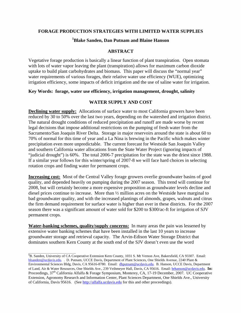
FORAGE CROP WATER USE Evapotranspiration (ET) and “Reference crop” ETo: The combination of air temperature, humidity, solar radiation and wind provide the energy to evaporate (E) water from the wet soil and to change the liquid water in the plant canopy into vapor that leaves the stomata in the underside of the leaves. This transpiration (T) helps to help cool the plant and allow for the uptake of carbon dioxide from the atmosphere for photosynthesis and carbohydrate production. The combination of these two is total water use for crop production, evapotranspiration or ET. The basic crop used to benchmark all others is a tall, well-watered, non-stressed cool season grass. This is called the “Reference Crop” and its water consumption is defined as Potential ET (ETo). California Irrigation Management Information Service (CIMIS) and estimating “normal year” ETo: The California Department of Water Resources has dedicated significant resources and full time staff to establish a network of statewide weather stations that use meteorological data to estimate ETo. Starting with the first stations in the early 1980’s there have been 208 stations installed with 134 currently active. Each station records hourly weather data and estimates of ETo. This data has provided the average ETo for the 18 zones shown in Figure 1 (Jones, et al., 1999). Because most of the irrigated acreage in California is blessed with very predictable weather during the growing season, especially from May through September when rainfall is not a factor, we can use these estimates of “normal year” ETo to get pretty close to expected crop water use over the season for a given area. The major alfalfa and forage production areas run from Zone 10 in the north (Tulelake) with an ETo of 49.1 inches to the Imperial Valley in the south, Zone 18, with a normal year ETo of 71.6 inches. The whole Central Valley covers Zones 12 to 16: for a normal year ETo of 53.3 to 62.5 in/yr, with most area at 53 to 58 inches. The example water use discussed in this paper will be based on Zone 15 with a normal year ETo of 57.9 inches. Ignoring the anomalous Zone 16 in Kings County, almost the
whole Central Valley floor is shown as Zones 14 and 15 – about 57 inches reference grass ETo per year.
Fig. 1. Current baseline ETo identified for 18 different zones across California. (Jones, et al.,1999.
California Irrigation Management Information System (CIMIS) Reference Evapotranspiration. Climate zone map. http://wwwcimis.water.ca.gov/cimis/images/etomap.jpg)
CIMIS weather data and irrigation management information can be accessed for free at:
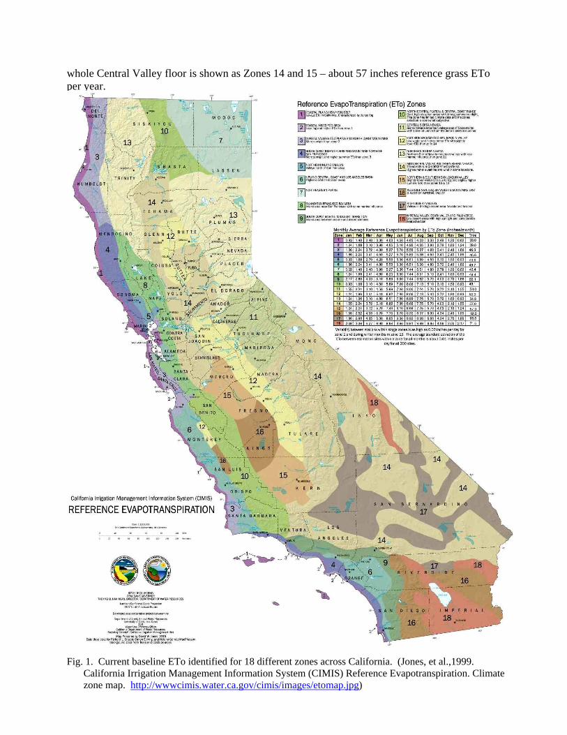
http://wwwcimis.water.ca.gov/cimis/welcome.jsp Crop coefficients (Kc) and average forage ET: Since most forage crops are planted dense and cover the ground like a pasture then it’s natural to assume that their ET would be the same as ETo, and as a first guess this isn’t too bad. But there are developmental differences due to initial seedling growth, physiology of the particular forage compared to pasture and cutting schedules. Basically, the crop coefficient, Kc, is the ratio of actual crop water use for a particular stage of growth compared to ETo. We have typical Kc values for the developmental stages of most crops. Crop ET is then calculated as follows:
ETcrop = ETo * Kc * Ef ETo = reference crop (tall grass) ET Kc = crop coefficient for a given stage of growth as a ratio of grass water use. May be
0 to 1.3, standard values are good starting point. Ef = an “environmental factor” to account for immature permanent crops, salinity,
etc. May be 0.1 to 1.1 depending on field. Usually 1 for good ground and water.
Table 1. Crop coefficients and calculated ET for various forage crops in the SJV. Pasture
2Kc of 0.95 takes into account reduced ET during cuttings over season.3Total of 3 cuttings. ET reduced for 1 to 2 weeks after cutting 7/15 and 9/1.4ET numbers in italics are evaporation losses from water at planting.
4Normal Year Crop ET (inches)
1Adapted from Pruitt, W.O., E. Fereres, K. Kaita, and R.L. Snyder. 1987. "Reference Evapotranspiration (ETo) for California." UC Bull. 1922. Pp. 12-13.
1Crop Coefficient Values (Kc)
*Jones, D.W., R.L. Snyder, S. Eching and H. Gomez-McPherson. 1999. California Irrigation Management Information System (CIMIS) Reference Evapotranspiration. Climate zone map, Dept. of Water Resources, Sacramento, CA.
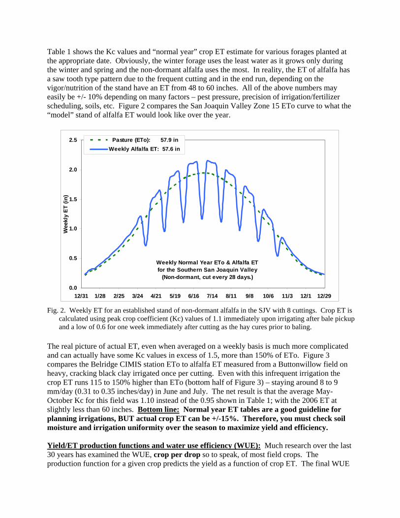
Table 1 shows the Kc values and “normal year” crop ET estimate for various forages planted at the appropriate date. Obviously, the winter forage uses the least water as it grows only during the winter and spring and the non-dormant alfalfa uses the most. In reality, the ET of alfalfa has a saw tooth type pattern due to the frequent cutting and in the end run, depending on the vigor/nutrition of the stand have an ET from 48 to 60 inches. All of the above numbers may easily be +/- 10% depending on many factors – pest pressure, precision of irrigation/fertilizer scheduling, soils, etc. Figure 2 compares the San Joaquin Valley Zone 15 ETo curve to what the “model” stand of alfalfa ET would look like over the year.
Weekly Normal Year ETo & Alfalfa ET for the Southern San Joaquin Valley
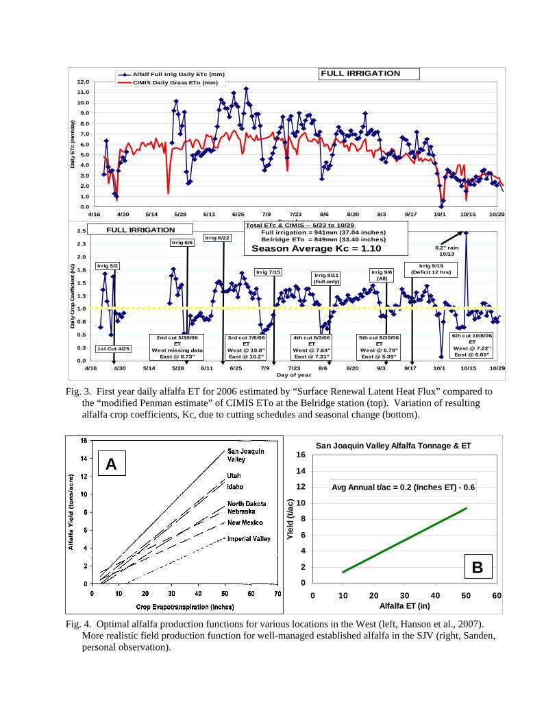
The real picture of actual ET, even when averaged on a weekly basis is much more complicated and can actually have some Kc values in excess of 1.5, more than 150% of ETo. Figure 3 compares the Belridge CIMIS station ETo to alfalfa ET measured from a Buttonwillow field on heavy, cracking black clay irrigated once per cutting. Even with this infrequent irrigation the crop ET runs 115 to 150% higher than ETo (bottom half of Figure 3) – staying around 8 to 9 mm/day (0.31 to 0.35 inches/day) in June and July. The net result is that the average May-October Kc for this field was 1.10 instead of the 0.95 shown in Table 1; with the 2006 ET at slightly less than 60 inches. Bottom line: Normal year ET tables are a good guideline for planning irrigations, BUT actual crop ET can be +/-15%. Therefore, you must check soil moisture and irrigation uniformity over the season to maximize yield and efficiency. Yield/ET production functions and water use efficiency (WUE): Much research over the last 30 years has examined the WUE, crop per drop so to speak, of most field crops. The production function for a given crop predicts the yield as a function of crop ET. The final WUE
Fig. 2. Weekly ET for an established stand of non-dormant alfalfa in the SJV with 8 cuttings. Crop ET is calculated using peak crop coefficient (Kc) values of 1.1 immediately upon irrigating after bale pickup and a low of 0.6 for one week immediately after cutting as the hay cures prior to baling.
0.0
1.0
2.0
3.0
4.0
5.0
6.0
7.0
8.0
9.0
10.0
11.0
12.0
4/16 4/30 5/14 5/28 6/11 6/25 7/9 7/23 8/6 8/20 9/3 9/17 10/1 10/15 10/29Day of year
Dai
ly E
Tc (m
m/d
ay)
Alfalf Full Irrig Daily ETc (mm)CIMIS Daily Grass ETo (mm)
FULL IRRIGATION
0.0
0.3
0.5
0.8
1.0
1.3
1.5
1.8
2.0
2.3
2.5
4/16 4/30 5/14 5/28 6/11 6/25 7/9 7/23 8/6 8/20 9/3 9/17 10/1 10/15 10/29Day of year
Dai
ly C
rop
Coe
ffici
ent (
Kc)
FULL IRRIGATION
Irrig 5/2
Total ETc & CIMIS -- 5/23 to 10/29 Full irrigation = 941mm (37.04 inches) Belridge ETo = 849mm (33.40 inches)
Season Average Kc = 1.10
Irrig 8/11(Full only)
Irrig 7/15
Irrig 6/22Irrig 6/6
Irrig 9/6(All)
1st Cut 4/25
5th cut 8/30/06ET
West @ 6.79"East @ 5.39"
4th cut 8/3/06ET
West @ 7.64"East @ 7.31"
3rd cut 7/6/06ET
West @ 10.8"East @ 10.2"
2nd cut 5/30/06ET
West missing dataEast @ 8.73"
Irrig 9/19(Deficit 12 hrs)
6th cut 10/8/06ET
West @ 7.22"East @ 6.85"
0.2" rain10/13
San Joaquin Valley Alfalfa Tonnage & ET
Avg Annual t/ac = 0.2 (Inches ET) - 0.6
0
2
4
6
8
10
12
14
16
0 10 20 30 40 50 60Alfalfa ET (in)
YIel
d (t/
ac)
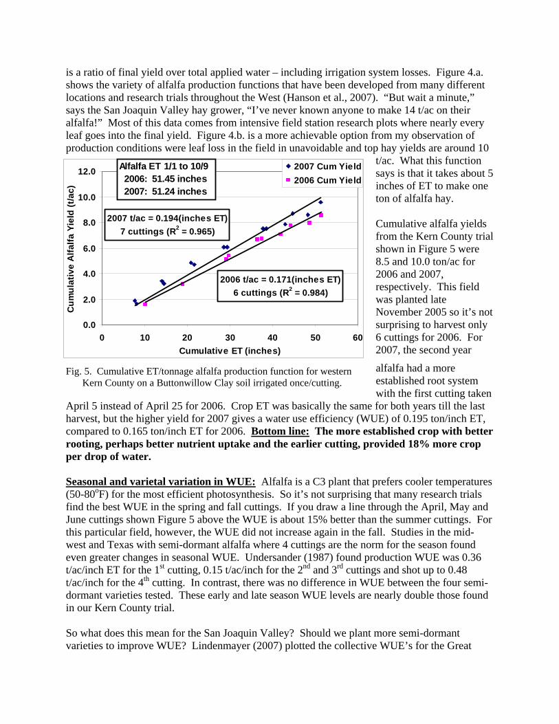
Fig. 4. Optimal alfalfa production functions for various locations in the West (left, Hanson et al., 2007). More realistic field production function for well-managed established alfalfa in the SJV (right, Sanden, personal observation).
Fig. 3. First year daily alfalfa ET for 2006 estimated by “Surface Renewal Latent Heat Flux” compared to the “modified Penman estimate” of CIMIS ETo at the Belridge station (top). Variation of resulting alfalfa crop coefficients, Kc, due to cutting schedules and seasonal change (bottom).
A
B
is a ratio of final yield over total applied water – including irrigation system losses. Figure 4.a. shows the variety of alfalfa production functions that have been developed from many different locations and research trials throughout the West (Hanson et al., 2007). “But wait a minute,” says the San Joaquin Valley hay grower, “I’ve never known anyone to make 14 t/ac on their alfalfa!” Most of this data comes from intensive field station research plots where nearly every leaf goes into the final yield. Figure 4.b. is a more achievable option from my observation of production conditions were leaf loss in the field in unavoidable and top hay yields are around 10
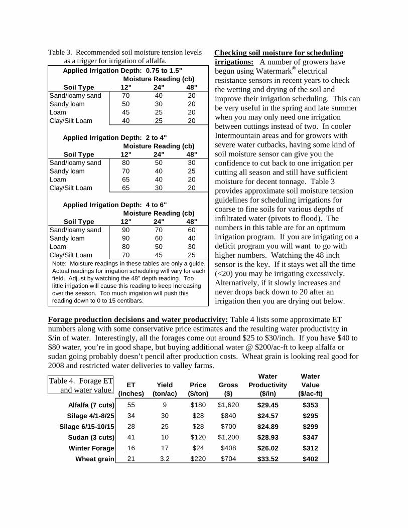
t/ac. What this function says is that it takes about 5 inches of ET to make one ton of alfalfa hay. Cumulative alfalfa yields from the Kern County trial shown in Figure 5 were 8.5 and 10.0 ton/ac for 2006 and 2007, respectively. This field was planted late November 2005 so it’s not surprising to harvest only 6 cuttings for 2006. For 2007, the second year
alfalfa had a more established root system with the first cutting taken
April 5 instead of April 25 for 2006. Crop ET was basically the same for both years till the last harvest, but the higher yield for 2007 gives a water use efficiency (WUE) of 0.195 ton/inch ET, compared to 0.165 ton/inch ET for 2006. Bottom line: The more established crop with better rooting, perhaps better nutrient uptake and the earlier cutting, provided 18% more crop per drop of water. Seasonal and varietal variation in WUE: Alfalfa is a C3 plant that prefers cooler temperatures (50-80oF) for the most efficient photosynthesis. So it’s not surprising that many research trials find the best WUE in the spring and fall cuttings. If you draw a line through the April, May and June cuttings shown Figure 5 above the WUE is about 15% better than the summer cuttings. For this particular field, however, the WUE did not increase again in the fall. Studies in the mid-west and Texas with semi-dormant alfalfa where 4 cuttings are the norm for the season found even greater changes in seasonal WUE. Undersander (1987) found production WUE was 0.36 t/ac/inch ET for the 1st cutting, 0.15 t/ac/inch for the 2nd and 3rd cuttings and shot up to 0.48 t/ac/inch for the 4th cutting. In contrast, there was no difference in WUE between the four semi-dormant varieties tested. These early and late season WUE levels are nearly double those found in our Kern County trial. So what does this mean for the San Joaquin Valley? Should we plant more semi-dormant varieties to improve WUE? Lindenmayer (2007) plotted the collective WUE’s for the Great
Alfalfa ET 1/1 to 10/9 2006: 51.45 inches 2007: 51.24 inches
Fig. 5. Cumulative ET/tonnage alfalfa production function for western Kern County on a Buttonwillow Clay soil irrigated once/cutting.
Plains and Intermountain West from 7 different authors and found a value of 0.136 ton/ac/inch – actually 25% less than the 2 year average for our Kern trial. This area of dormancy on the impact of WUE needs more research for California. What we do know is that we can withhold summer irrigations and still bring the stand back. Frate, et.al (1988) found that you could cutoff irrigation in July and August – losing 1 to 2 tons of the summer cutting. Irrigating in September, October or even the spring of the following year brought the stand back so that there was no impact on yields the following year. This is virtually the same result as our Kern County trial. However, summer fallow trials in the very hot southern valleys of Imperial, Palo Verde and Mesa Verde showed significant stand damage due to excessive heating of the crowns. Bottom line: WUE in alfalfa is best in the spring and the fall. Average full season WUE for semi-dormant hay varieties is about the same as non-dormant varieties in the Central Valley, but fall and spring WUE may be better for the semi-dormant cultivars. Summer irrigations can be withheld without long-term stand loss (except in Imperial Valley). Some fields overlying low salinity perched water in the Intermountain Area have maintained full production even without surface irrigation (Orloff, 2003). Actual field irrigation distribution uniformity (DU), applied water and yield: DU is defined as the average infiltration depth of water for the “low quarter” (tail end or low pressure 25%) of the field, and is expressed as a percentage:
DU (%) = 100 *
“low quarter” infiltration
Average field infiltration
Figure 6 illustrates how this plays out in your crop rootzone for a field DU of about 80% with some deficit irrigation on the end. To insure that no more than about 12% of the field gets less than full ET, you divide the expected ET of the crop by the field application DU. So if the alfalfa has a 50 inch requirement for ET and the field has an 80% DU then the applied water required = 50/0.8 = 62.5 inches. That’s an extra foot of water! If the DU is 90% (which is achievable with quarter mile runs, the right on-flow rate, a tail water return system and proper scheduling) then applied water = 50/0.9 = 55.5 inches. So you can save 7 inches of water by improving the uniformity and still adequately water the field.
0 –
0.5 –
1.0 –
1.5 –
2.0 –
Stressed plant growthToo little water
Possible stressN leaching, water logging
Infiltration @ 6 hrs
Infiltration @ 12 hrs
Infiltration @ 18 hrs
Infiltration @ 24 hrs
Head
Tail – no leaching
Roo
tzon
e D
epth
(m)
Deep percolation – lost water & N fertilizer
0 –
0.5 –
1.0 –
1.5 –
2.0 –
0 –
0.5 –
1.0 –
1.5 –
2.0 –
Stressed plant growthToo little water
Stressed plant growthToo little water
Possible stressN leaching, water logging
Possible stressN leaching, water logging
Infiltration @ 6 hrs
Infiltration @ 12 hrs
Infiltration @ 18 hrs
Infiltration @ 24 hrs
Head
Tail – no leaching
Roo
tzon
e D
epth
(m)
Deep percolation – lost water & N fertilizer
Fig. 6. Cross-section of crop rootzone during a 24 hour furrow irrigation.
Continuing with alfalfa for the moment, 12 ton yields in the SJV usually come from small plots at ag research stations where irrigations were very short and nearly 100% uniform. Actual field DU may range from a low of 65% for a coarse sandy border flood system with no tail water return to 95% for sub-surface drip or new pivots and linear move sprinklers in low wind conditions. In Kern County from 1988 to 2003, the average DU for border systems was 80% (Brian Hockett, unpublished data), ranging from 37 to 100%. (A 100% DU is theoretically possible on a cracking, sealing clay soil.) A total of 27 out of 80 borders evaluated had 90 to 100% DU. The average DU for 40 linear move sprinkler systems tested was only 77%. So how does this play out in a production field. Figure 7 is a hypothetical alfalfa field that can yield 8.5 ton for the areas in the field where the irrigation schedule is just right. But this field does not drain well and where there is too much water you lose stand and yield to scald and phytophthora (the blocked end of the border and some of the head end in this case). Obviously, where the infiltration is too little (about 900 to 1150 feet from the head) the tonnage also decreases. Table 2 gives 3 scenarios using the production function in Figure 7 for a 70, 80 or 90% DU where the applied water for the season is 42, 48, 54 or 60 inches. Remember that a 55 inch water application is about right for a 50 inch ET requirement and a field with 90% DU.
Qtr Irrig by Avg Depth (in) Qtr Yield by Avg Depth (t/ac)
Field Average Yield (t/ac):
Field Average Yield (t/ac):
Field Average Yield (t/ac):
Yield (t/ac) = -0.0096x2 + 1.0004x - 17.491
R2 = 0.9789
5.0
5.5
6.0
6.5
7.0
7.5
8.0
8.5
9.0
35 45 55 65Applied water(in)
Alfa
lfa Y
ield
(t/a
c)
If we apply 54 inches of water and we have a DU of 70% then the driest area of the field only gets 38 inches for the season and the wettest gets 70 inches. Looking at the right side of the table (Qtr Yield by Avg Depth) under the 54 inch column you can see that only ¼ of the field gets the right amount of water and hits the 8.5 t/ac. Half of the field yields less than 6.5 t/ac. So the average field yield is 7.3 t/ac. Improve the DU to 90% with tail water return and higher on-flows to reduce infiltration and water-logging you bump the whole field up to 8.4 t/ac with the same 54 inches of water! Bottom line: improving irrigation DU pays.
Table 2. Average seasonal applied water on the wettest to driest areas of an alfalfa field and the resulting yield for those areas for for various irrigation amounts and DU.
Fig. 7. Alfalfa production function for field sensitive to waterlogging.
Checking soil moisture for scheduling irrigations: A number of growers have begun using Watermark® electrical resistance sensors in recent years to check the wetting and drying of the soil and improve their irrigation scheduling. This can be very useful in the spring and late summer when you may only need one irrigation between cuttings instead of two. In cooler Intermountain areas and for growers with severe water cutbacks, having some kind of soil moisture sensor can give you the confidence to cut back to one irrigation per cutting all season and still have sufficient moisture for decent tonnage. Table 3 provides approximate soil moisture tension guidelines for scheduling irrigations for coarse to fine soils for various depths of infiltrated water (pivots to flood). The numbers in this table are for an optimum irrigation program. If you are irrigating on a deficit program you will want to go with higher numbers. Watching the 48 inch sensor is the key. If it stays wet all the time (<20) you may be irrigating excessively. Alternatively, if it slowly increases and never drops back down to 20 after an irrigation then you are drying out below.
Forage production decisions and water productivity: Table 4 lists some approximate ET numbers along with some conservative price estimates and the resulting water productivity in $/in of water. Interestingly, all the forages come out around $25 to $30/inch. If you have $40 to $80 water, you’re in good shape, but buying additional water @ $200/ac-ft to keep alfalfa or sudan going probably doesn’t pencil after production costs. Wheat grain is looking real good for 2008 and restricted water deliveries to valley farms.
Applied Irrigation Depth: 4 to 6"Moisture Reading (cb)
Soil Type 12" 24" 48"Sand/loamy sand 90 70 60Sandy loam 90 60 40Loam 80 50 30Clay/Silt Loam 70 45 25Note: Moisture readings in these tables are only a guide. Actual readings for irrigation scheduling will vary for each field. Adjust by watching the 48" depth reading. Too little irrigation will cause this reading to keep increasing over the season. Too much irrigation will push this reading down to 0 to 15 centibars.
Table 3. Recommended soil moisture tension levels as a trigger for irrigation of alfalfa.
Table 4. Forage ET and water value.
Options for saline water use on forage crops: Table 5 lists most forage crops in order of increasing salinity tolerance with berseem as the most sensitive and tall wheatgrass as most tolerant. What this means is that if you have a source of drain water at an EC of 4 dS/m and you irrigate silage or alfalfa you can lose 25% of the potential yield for that field and the ET will also decrease. On the other hand if you plant winter wheat for grain you will not lose yield. Again, these values are only guidelines and will go up or down depending on some varietal differences, existing salt levels in the soil and the ratio of sodium to calcium in the irrigation water. Table 5 Crop tolerance and yield potential of selected crops as influenced by irrigation
water salinity (ECw) or soil salinity (ECe)1 (Ayers and Westcott, 1985) YIELD POTENTIAL2
Wheatgrass, tall (Agropyron elongatum) 7.5 5.0 9.9 6.6 13 9.0 19 13 31 21 1 Adapted from Maas and Hoffman (1977) and Maas (1984). These data should only serve as a guide to relative tolerances among crops. Absolute tolerances vary depending upon climate, soil conditions and cultural practices. In gypsiferous soils, plants will tolerate about 2 dS/m higher soil salinity (ECe) than indicated but the water salinity (ECw) will remain the same as shown in this table.
2 ECe means average root zone salinity as measured by electrical conductivity of the saturation extract of the soil, reported in deciSiemens per metre (dS/m) at 25°C. ECw means electrical conductivity of the irrigation water in deciSiemens per metre (dS/m). The relationship between soil salinity and water salinity (ECe = 1.5 ECw) assumes a 15–20 percent leaching fraction and a 40-30-20-10 percent water use pattern for the upper to lower quarters of the root zone. These assumptions were used in developing the guidelines in Table 1.
3 The zero yield potential or maximum ECe indicates the theoretical soil salinity (ECe) atwhich crop growth ceases.
4 Barley and wheat are less tolerant during germination and seeding stage; ECe should not exceed 4–5 dS/m in the upper soil during this period.
REFERENCES Ayers, R.S. and D.W. Westcot. 1985. Water Quality for Agriculture. FAO Irrigation and Drainage Paper 29 Rev. 1, Reprinted 1989, 1994. http://www.fao.org/DOCREP/003/T0234E/T0234E00.htm Frate, C., B. Roberts, and R. Sheesley. 1988. Managing alfalfa production with limited irrigation water. Proceedings, 18th California Alfalfa Symposium, 7–8 Dec 1988. Modesto, CA. Univ. California, Davis, Coop. Ext. pp. 7–13 Hanson, B.R., K.M. Bali, B.L. Sanden. 2007. Irrigated Alfalfa Production in Mediterranean and Desert Climates. Technical manual companion to Arid Land Alfalfa Manual. Univ. California, Davis, Dept. Land, Air and Water Resources, UC ANR Publication to be announced. 36 pp. Jones, D.W., R.L. Snyder, S. Eching and H. Gomez-McPherson. 1999. California Irrigation Management Information System (CIMIS) Reference Evapotranspiration. Climate zone map, Dept. of Water Resources, Sacramento, CA. http://wwwcimis.water.ca.gov/cimis/images/etomap.jpg Lindenmayer, B.R. and N. Hansen. 2007. Alfalfa Growth Responses to Water and Partial Season Irrigation Strategies. ASA-CSSA-SSSA International Annual Meetings, Nov. 4-8, New Orleans, LA. Abstract 201-5. Orloff, S., D. Putnam, B. Hanson, and H. Carlson. 2003. Controlled deficit irrigation of alfalfa: Opportunities and Pitfalls. Proceedings, 33rd California Alfalfa Symposium, 17–19 Dec 2003. Monterey, CA. Univ. California, Davis, Coop. Ext. pp. 39–52. Undersander, D.J. (1987) Alfalfa (Medicago sativa L.) Growth Response to Water and Temperature. Irrig. Sci. 8: 23-33 Additional Irrigation Management Resources Determining Daily Reference Evapotranspiration (ETo). UC Publication 21426. Drought Irrigation Strategies for Deciduous Orchards. UC Publication 21453. Drought Tips for Vegetable and Field Crop Production. UC Publication 21466. Grattan, S.R., Bowers, W., Dong, A., Snyder, R., Carroll, J. J. and George, W. 1998. New crop coefficients estimate water use of vegetables, row crops. California Agriculture, Vol 52, No. 1. Irrigation Scheduling: A Guide for Efficient On-Farm Water Management. UC Publication 21454. Using Reference Evapotranspiration (ETo) and Crop Coefficients to Estimate Crop Evapotranspiration (ETc) for Agronomic Crops, Grasses, and Vegetable Crops. UC Publication 21427. Using Reference Evapotranspiration (ETo) and Crop Coefficients to Estimate Crop Evapotranspiration (ETc) for Trees and Vines. UC Publication 21428.