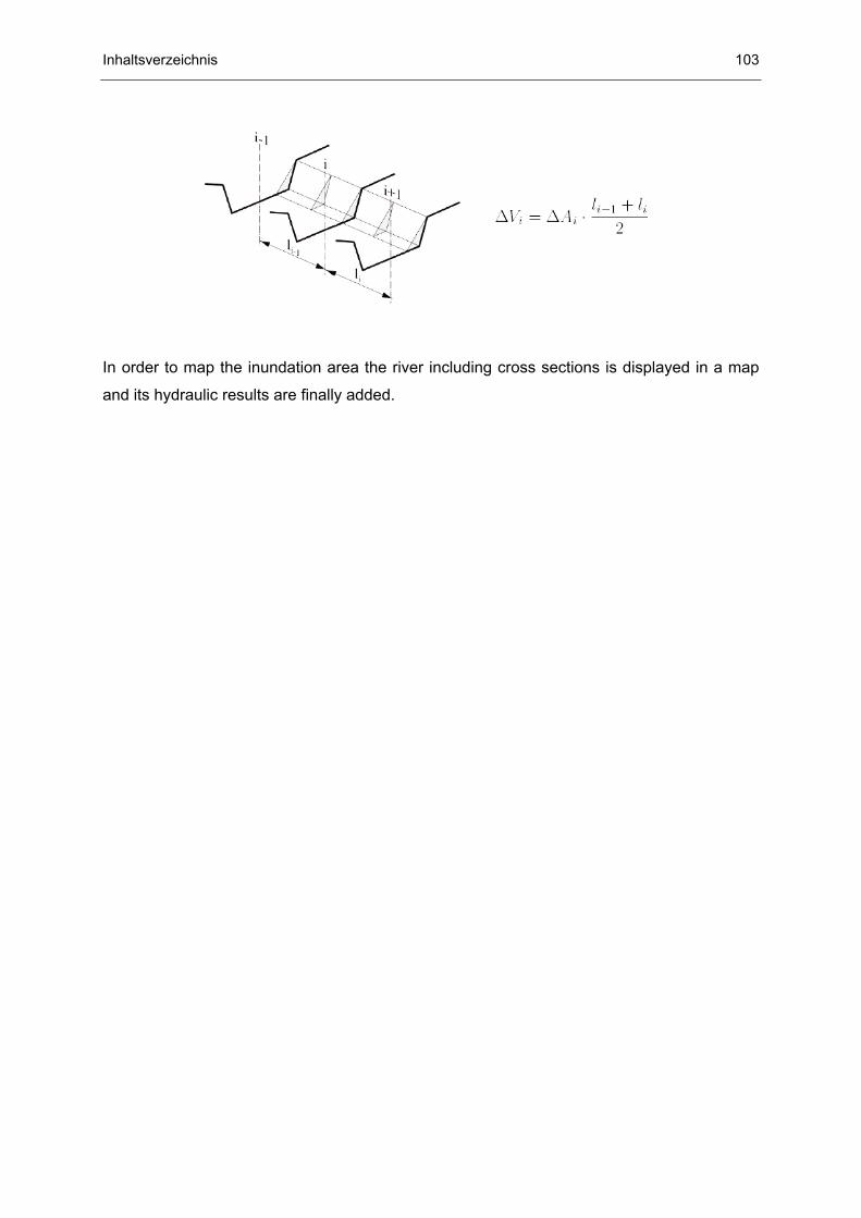
1D - Hydraulic Prof. Dr.-Ing. Miodrag Jovanovic UNIVERSITY OF BELGRADE Faculty of Civil Engineering Prof. Dr.-Ing. Erik Pasche Dr.-Ing. Markus Töppel Dipl.-Ing. Monika Donner TECHNISCHE UNIVERSITÄT HAMBURG-HARBURG Institut für Wasserbau Denickestraße 22 , 21073 Hamburg Hamburg, 29. Juni 2006
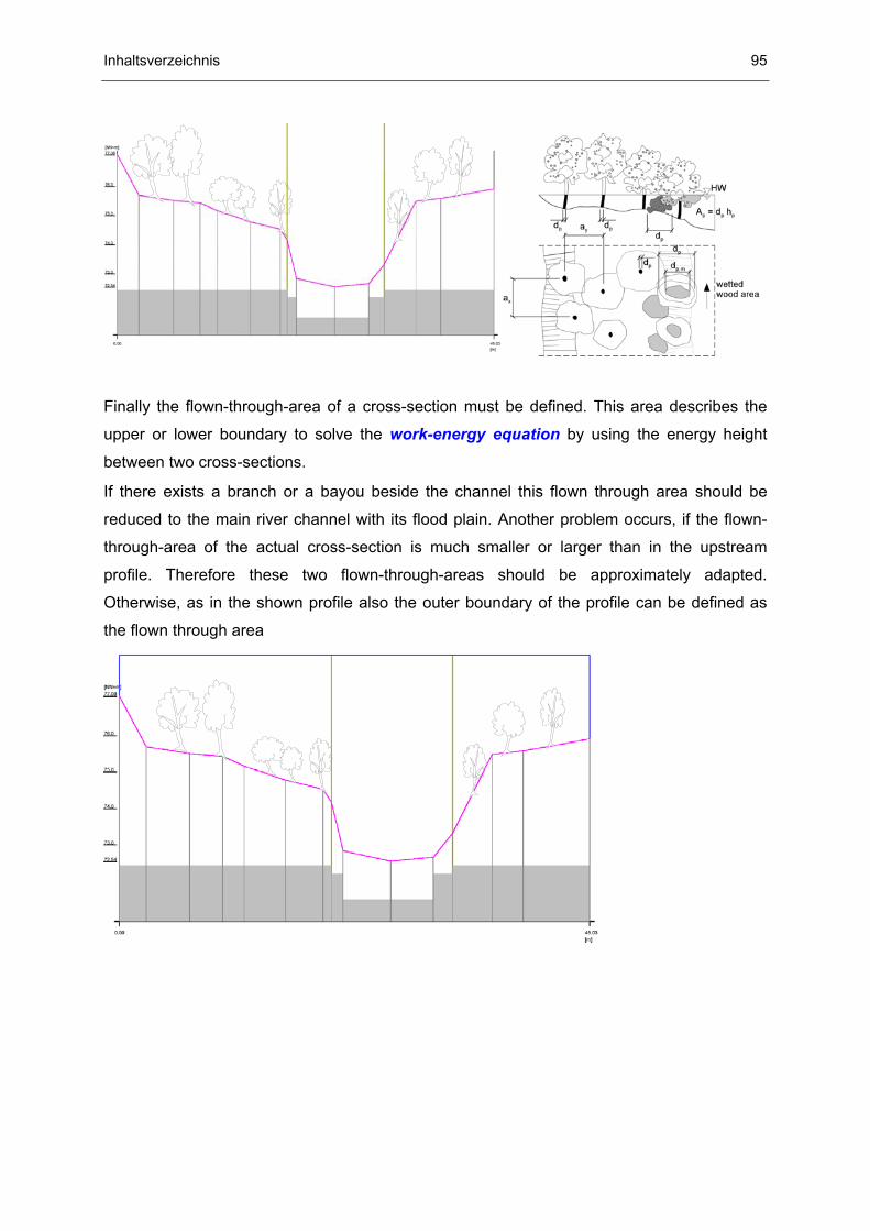
Transcript
1D - Hydraulic
Prof. Dr.-Ing. Miodrag Jovanovic UNIVERSITY OF BELGRADE
Faculty of Civil Engineering
Prof. Dr.-Ing. Erik Pasche Dr.-Ing. Markus Töppel Dipl.-Ing. Monika Donner
TECHNISCHE UNIVERSITÄT HAMBURG-HARBURG
Institut für Wasserbau Denickestraße 22 , 21073 Hamburg
Hamburg, 29. Juni 2006
III
Contents
Contents III
1 Introduction - 1D hydraulic simulation 1
2 Hydraulic processes 2
3 Basic equations 6
3.1 Continuity equation (conservation of mass) 6 3.2 The impulse-momentum equation 7 3.3 BERNOULLI’s equation (equation of energy conservation) 7 3.4 Coefficients of energy and momentum 9
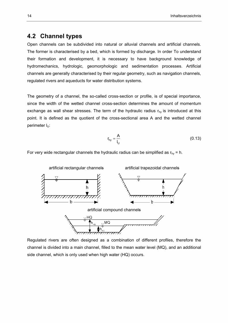
4 Open channel flow 13
4.1 The flow phenomena in natural rivers 13 4.2 Channel types 14 4.3 Flow formulas 15
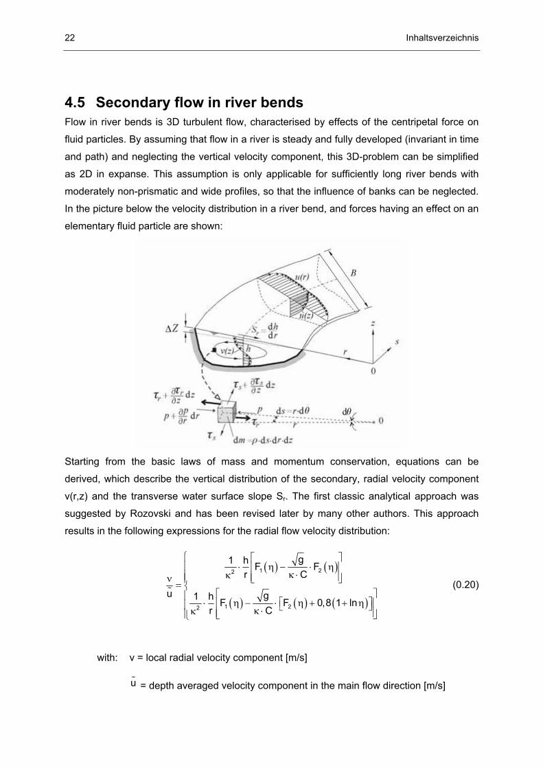
4.3.1 The Friction coefficient λ Darcy-Weisbach - Law 16 4.4 Velocity distribution over depth 17 4.5 Secondary flow in river bends 22
5 Channel roughness 28
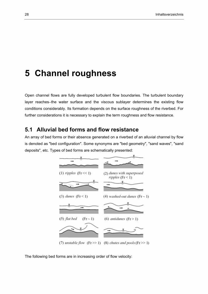
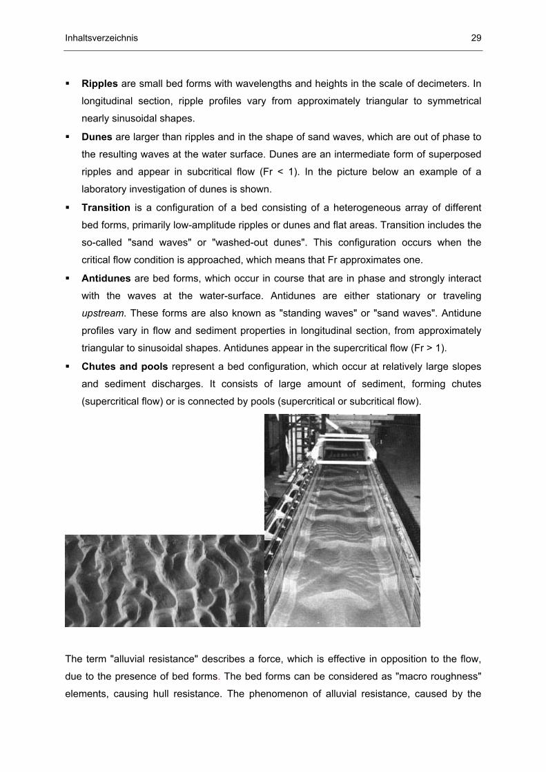
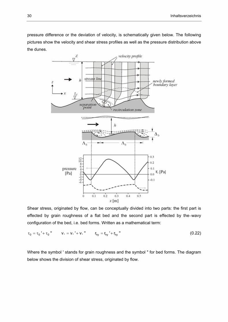
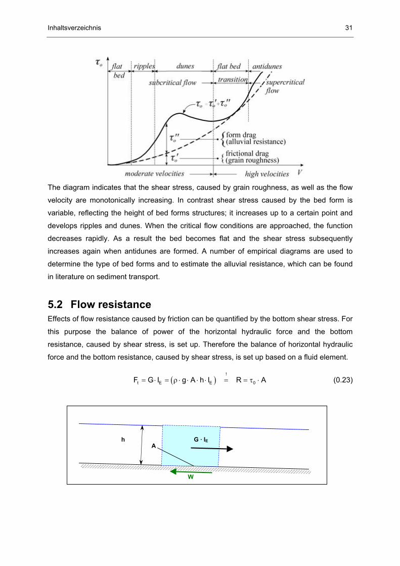
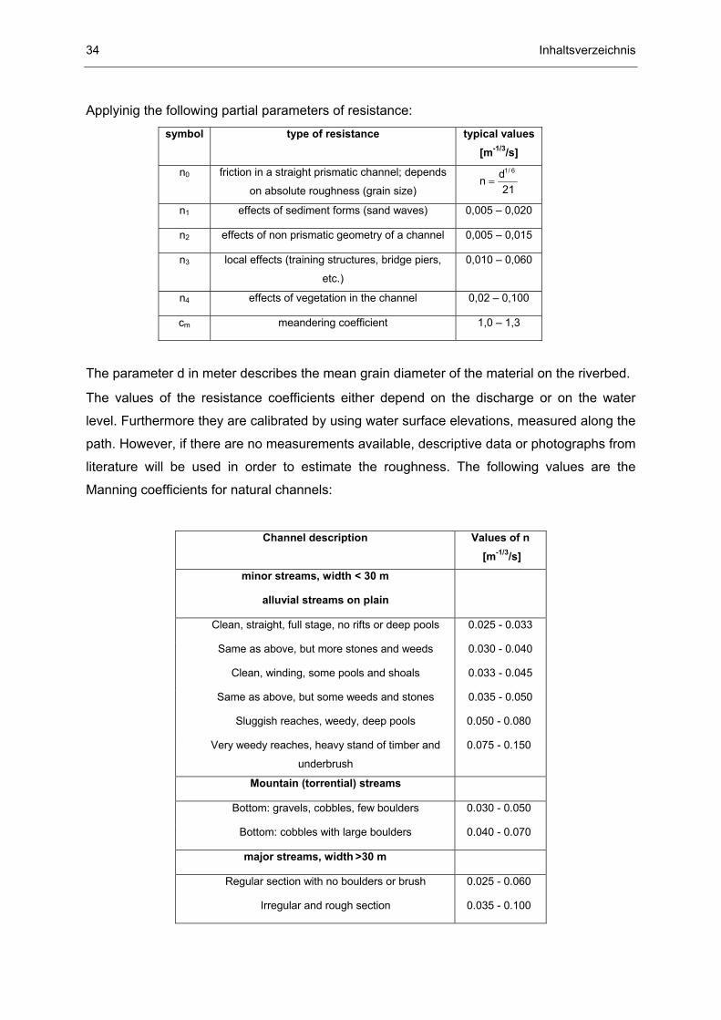
5.1 Alluvial bed forms and flow resistance 28 5.2 Flow resistance 31
5.3.2 Consideration of additional influences in semi-natural flowing water 41 5.3.3 Meandering 42
5.4 Friction coefficient for roughness caused by vegetation 42 5.4.1 Friction coefficient for flooded vegetation (small vegetation) 43 5.4.2 Friction coefficient for immersed vegetation (middle and high vegetation) 47
5.5 Friction coefficient as a function of the cross-section 49 5.5.1 Friction coefficient for layering of roughness 50 5.5.2 Friction coefficient for partitioned cross-sections 52
5.6 Composite roughness based on Manning 56 5.7 Hydraulic parameters of complex cross-sections 58
6 Flow over and against hydraulic structures 62
6.1 Weirs 63 6.1.1 Weirs with free (critical) overflow 64 6.1.2 Weirs with subcritical overflow 68 6.1.3 Submerged weirs (flow over crest) 69 6.1.4 Weirs with different crest heights 70
6.2 Bridges 71 6.2.1 Free discharge at a bridge 72 6.2.2 Dammed-in bridge structure with a free discharge under the bridge 73 6.2.3 Dammed-in bridge structure with backwater (subcritical discharge) 75 6.2.4 Submerged bridge structure with supercritical flow 75 6.2.5 Dammed-in bridge structure with subcritical overflow 77 6.2.6 Effects of bridge constrictions on water levels 78
6.3 Pipes and outlets 83 6.3.1 Attrition of hydraulic energy 83 6.3.2 Solution for pipe flow 84
7 Retention 86
8 Simulation with Kalypso 1D 88
8.1 Background of KALYPSO-1D 89 8.2 Preprocessing in KALYPSO-1D 90
8.2.1 Profile data and geographical data 91 8.2.2 Hydraulic parameters 93 8.2.3 Hydraulic structures 96 8.2.4 Measured hydraulic data and design floods 99
Inhaltsverzeichnis V
8.3 Simulation in KALYPSO-1D 99 8.3.1 Boundary Conditions 100 8.3.2 Options for the simulation of discharge events 100
8.4 Post-processing in KALYPSO-1D 101
9 Application 104
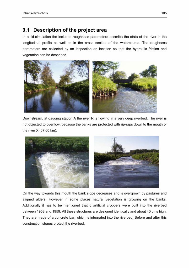
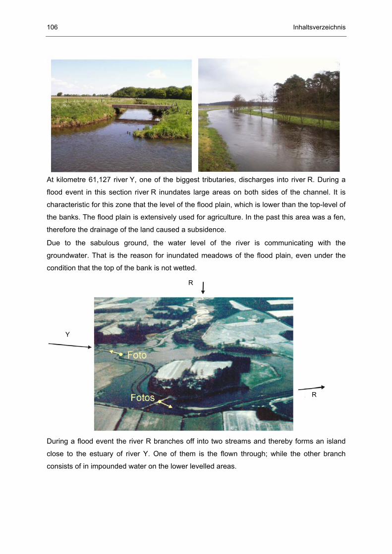
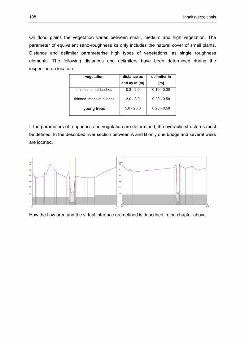
9.1 Description of the project area 105 9.2 Building up the 1D-model 107 9.3 Calibration 109 9.4 Design flood events of river R 111
1
1 Introduction - 1D hydraulic simulation
Nowadays the natural design of a watercourse is the main target. This philosophy is based
on the idea of an overall water management. In the past rivers were regarded as channels
with sewer function. Therefore they were regulated and the vegetation of the flood plain and
in the water transition area was removed. These measures caused an increase of flood
discharge and as a consequence the water level rose, furthermore the bed load and
sediment is scoured during strong floods.
Dealing with ecological water management the natural watercourse should be preserved as
naturally as possible. The conservation of the integrated water body in its environment,
including biological aspects as well as scenic beauties, is one of the basic principles. This
includes the preservation of vegetation and naturally deformed bed load structures in order to
preserve a habitat for fauna and flora. These rough elements cause more complex flow
processes. In order to display these interactions between vegetation and rough elements in
rivers, hydraulic models are used.
Quite a fast method of calculating the flow pattern in open channels is the one dimensional,
steady simulation of the water level. This method reduces multidimensional, natural
processes to one-dimensional questions by adopting a constant velocity and movement of
the water along the flow path.
If the movement of a water body is reduced to a one-dimensional problem, all calculated
results will be average values. That means the parameter is averaged over the water depth
and the cross section. Only the alteration of the considered parameters, such as the velocity
of the water body, along a streamtube is calculated. Of course such a 1D-model is also
applicable for channels, embanked watercourses and pipe flow processes. Primarily the
hydraulic processes are considered before the basic equations for one-dimensional flow
problems are set up.
2 Inhaltsverzeichnis
2 Hydraulic processes
Hydraulics is an engineering science pertaining to liquid pressure and flow. Hydraulic
processes are used to convert a volume of water moving down a channel. To study the
movement of floodwater through a stream and on a flood plain is the main target. The
hydraulic study determines the flood elevations, velocities and the size of flood plains at each
cross section for a range of flood flow frequencies. These hydraulic processes are normally
displayed by using computer models. These flood elevations are the primary data source
used by engineers to map a flood plain.
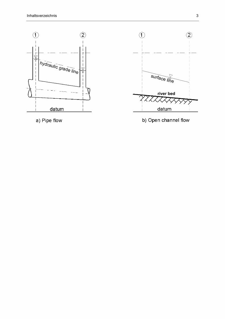
The movement of fluids is possible in systems with:
a closed cross section (pipe flow):
A pressure-resistant casing encloses a moving fluid in a pipe generally. The pressure
head of the fluid can be determined by piezometer.
a free surface (open channel flow):
The open channel flow is characterised by a combination of a firm and a fluid boundary layer.
The latter is to be understood as an interface between two fluids of different density.
The most important part of the channel current in practice is the water flow on the earth's surface. The characteristic of this special case is the interface between water and air at the
water surface. It is essential that the water pressure at the water surface is identical to the
atmospheric pressure. The water surface can be regarded as a surface of constant pressure.
It is generally accepted as a reference and set to zero.
Inhaltsverzeichnis 3
river bed
4 Inhaltsverzeichnis
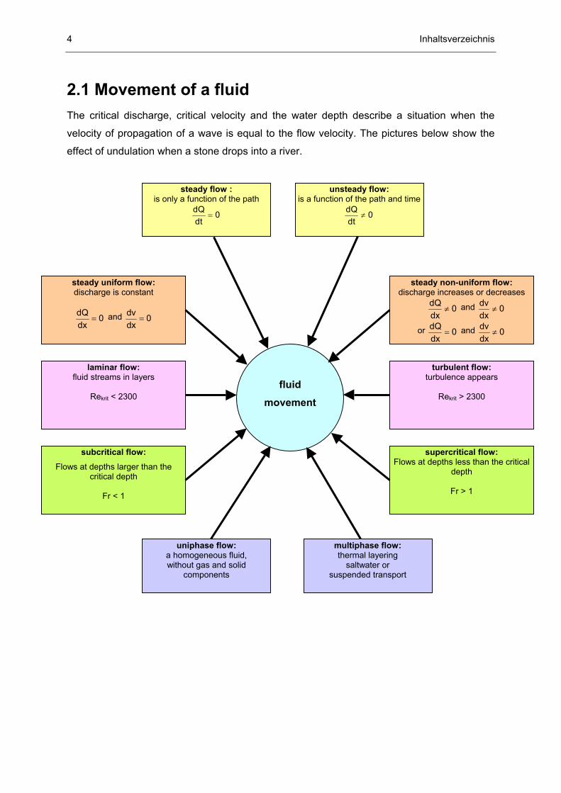
2.1 Movement of a fluid The critical discharge, critical velocity and the water depth describe a situation when the
velocity of propagation of a wave is equal to the flow velocity. The pictures below show the
effect of undulation when a stone drops into a river.
steady flow : is only a function of the path
=dQ 0dt
unsteady flow: is a function of the path and time
≠dQ 0dt
steady uniform flow: discharge is constant
=dQ 0dx
and =dv 0dx
steady non-uniform flow: discharge increases or decreases
≠dQ 0dx
and ≠dv 0dx
or =dQ 0dx
and ≠dv 0dx
laminar flow: fluid streams in layers
Rekrit < 2300
turbulent flow: turbulence appears
Rekrit > 2300
supercritical flow: Flows at depths less than the critical
depth
Fr > 1
subcritical flow: Flows at depths larger than the
critical depth
Fr < 1
multiphase flow: thermal layering
saltwater or suspended transport
uniphase flow: a homogeneous fluid, without gas and solid
components
fluid
movement
Inhaltsverzeichnis 5
standing water subcritical discharge critical discharge supercritical discharge
v 0Fr 0
==
gr0 v c v
Fr v / c 1
≠ < =
= < gr0 v c v
Fr v / c 1
≠ = =
= = gr0 v c v
Fr v / c 1
≠ > =
= >
The relationship between h and hE for a constant discharge Q can be displayed in a diagram.
In reference to the diagram, the following statements can be made:
Under a given discharge Q a minimum height of energy hE,min exists . This statement is
known as extremal principle.
With an existing specific energy hE larger than hE,min, two conditions are possible:
• Low water depth h, high flow velocity v:
This flow is supercritical. Enormous stress at the bottom is the result. Interferences do
not spread out upstream, therefore the flowage is only calculated for a downstream flow.
• Great water depth h, low flow velocity v:
This flow is subcritical. This type of movement is often found in open channels and
rivers. Interferences such as a cross-section constriction have an effect on the upstream
flow. The flowage is calculated for the upstream flow.
6 Inhaltsverzeichnis
3 Basic equations
The solution of the water shallow equation in an open channel is done by an energy theorem.
This equation can be derived from the equation of the conservation of momentum, equation
of energy conservation and the continuity equation. Primarily it is necessary to understand
the difference of these three equations. They are based on the assumption that the fluid is
homogeneous and incompressible, consequently the density is constant, and furthermore the
equations are based on steady flow processes.
3.1 Continuity equation (conservation of mass) The main conclusion of this equation: The discharge dQ in a streamtube has to be constant,
irrespective of the path.
= ⋅ =v dA constdQ (0.1)
The basic idea of this fundamental law of nature is the conservation of mass (input = output)
along the path between two sections. There are numerous specialised books, which discuss
the derivation of the three-dimensional continuity, however in this case only the one-
dimensional problem is discussed.
Inhaltsverzeichnis 7
3.2 The impulse-momentum equation It derives from Newton’s equation of momentum. The external forces on the frontal areas of a
control volume are contrasted.
( )= ⋅ ⇒ = ρ ⋅⋅ ⋅ β − β2 2 1 1dm dv QdF dt F v v (0.2)
The force F is given as a calculated parameter depending on the discharge Q and the
velocity v. The factor β is defined as the BOUSSINESQUE parameter, which describes the
inhomogeneous distribution of the velocity. For a homogeneous velocity distribution the
factor is set to 1.
datum
control volume
fluid body
3.3 BERNOULLI’s equation (equation of energy conservation)
The energy theorem means: “The total energy of a body, which is neither supplied by energy
nor is energy extracted from the outside is constant. The stored energy appears in different
states. Transformations from one state to another within a body are possible. Certainly, this
theorem also applies for fluid flow.
BERNOULLI’ s equation gathers the height of energy between two cross-sections. Based on
the conservation of energy, this height of energy H can be derived:
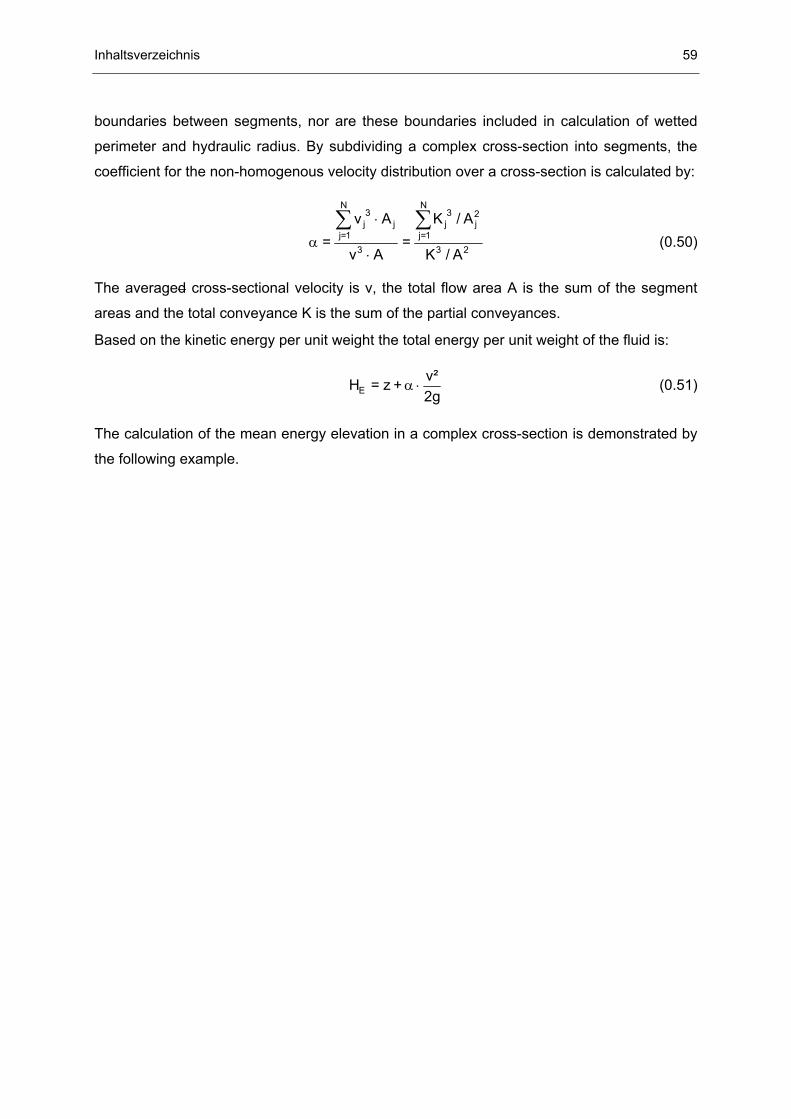
( )= ⋅ ⇒ = α ⋅
⋅ + + γ
22
0p
dm d v H z1 vdF ds2 2g
(0.3)
8 Inhaltsverzeichnis
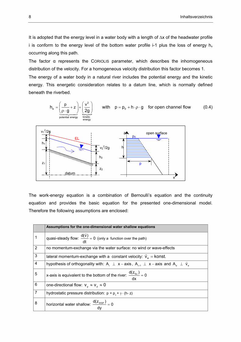
It is adopted that the energy level in a water body with a length of ∆x of the headwater profile
i is conform to the energy level of the bottom water profile i-1 plus the loss of energy hv
occurring along this path.
The factor α represents the CORIOLIS parameter, which describes the inhomogeneous
distribution of the velocity. For a homogeneous velocity distribution this factor becomes 1.
The energy of a water body in a natural river includes the potential energy and the kinetic
energy. This energetic consideration relates to a datum line, which is normally defined
beneath the riverbed.
= + +
= + ⋅ ρ ⋅ ρ ⋅
2
e 0
kinetic potential energyenergy
p vzh with p p h g for open channel flow
g 2g (0.4)
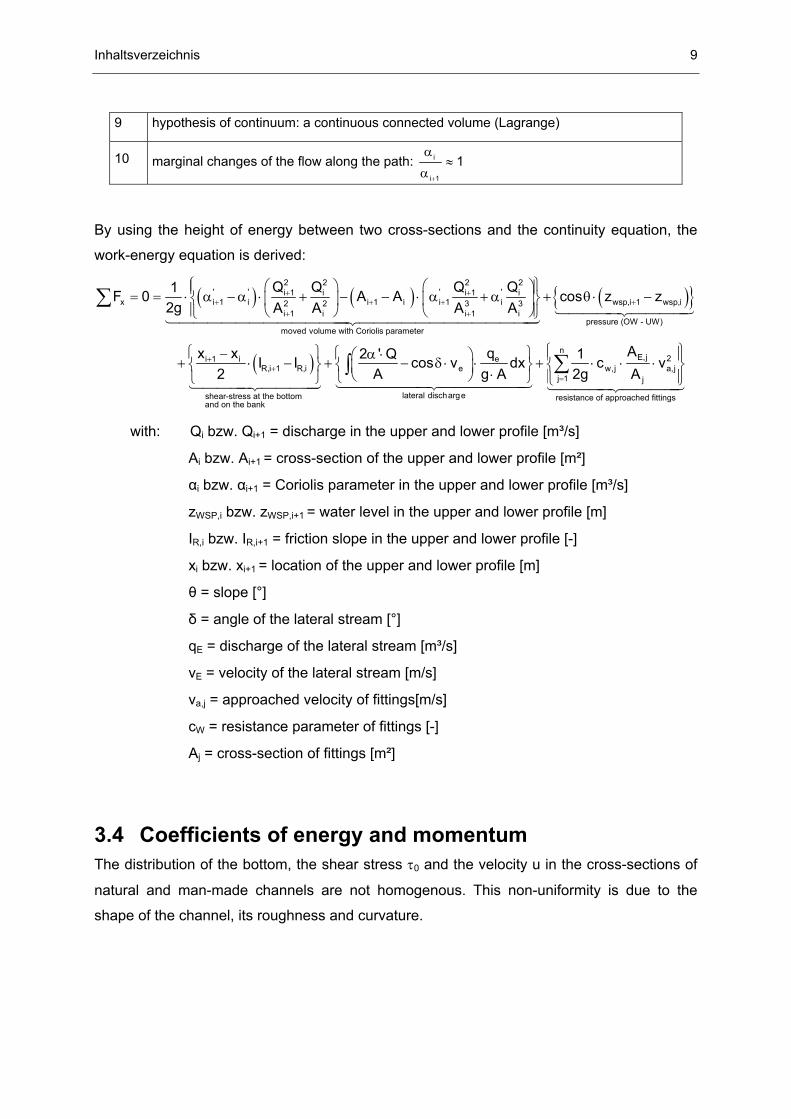
The work-energy equation is a combination of Bernoulli’s equation and the continuity
equation and provides the basic equation for the presented one-dimensional model.
Therefore the following assumptions are enclosed:
Assumptions for the one-dimensional water shallow equations
1 quasi-steady flow: =d(v)
0dt
(only a function over the path)
2 no momentum-exchange via the water surface: no wind or wave-effects
3 lateral momentum-exchange with a constant velocity: =ev konst.
4 hypothesis of orthogonality with: ⊥ −iA x axis , + ⊥ −i 1A x axis and ⊥e eA v
5 x-axis is equivalent to the bottom of the river: =Sod(z )0
In literature the term absolute hydraulic roughness k is used. This roughness is identical to
the equivalent sand roughness ks as described above. In general the symbol k is only used
for the geometrical (measurable) roughness.
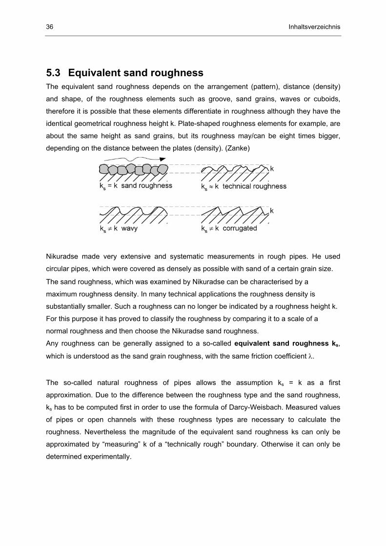
38 Inhaltsverzeichnis
5.3.1 Hydraulic effect of roughness The resistance of a boundary does not only depend on the equivalent sand roughness ks, but
also on the characteristic dimension of the cross-section and shape. Such a dimension of a
cross-section could for example be the flow depth in open channel hydraulics or the pipe
diameter in pipe hydraulics. With respect to the general use the hydraulic diameter dhy (with
hy hyd 4r= ) is used as the characteristic dimension of the cross-section. The quotient of the
equivalent sand roughness ks and the hydraulic diameter dhy is called the relative roughness ks/dhy.
The flow resistance, characterised by the friction coefficient λ, can be very different in spite of
the same relative roughness s hyk / 4r . Furthermore it depends on the grade of turbulence of
in the flow (intensity of the transverse movements of the fluid particles) specified by the
Reynolds number Re. The Reynolds numbers, occurring in natural flow conditions, are much
larger than the critical Reynolds number Rekrit = 2300. Therefore the flow in natural rivers is
usually turbulent.
The following types of roughness can be differentiated:
• hydraulically smooth
• transitional behavior
• hydraulically rough
• hydraulically extremely rough
Hydraulically smooth
The flow close to the boundary has a small (but turbulent) Reynolds number and is
dominated by the viscous sublayer (tenacity). If its thickness δ of the viscous sublayer is
larger than the height of the roughness elements k, the viscous sublayer will covers all
roughness elements and act as a “lubricant” between the boundary and the turbulent flow. As
a result the roughness of the bed has no influence on the turbulent boundary layer. The flow
resistance, characterised by the friction coefficient λ, only depends on the Reynolds number
Re.
1 2,512,03 logRe
= − ⋅
λ ⋅ λ (0.26)
Inhaltsverzeichnis 39
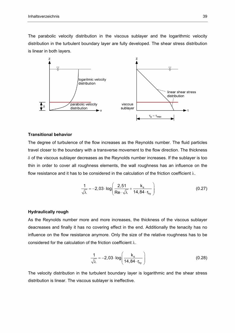
The parabolic velocity distribution in the viscous sublayer and the logarithmic velocity
distribution in the turbulent boundary layer are fully developed. The shear stress distribution
is linear in both layers.
Transitional behavior
The degree of turbulence of the flow increases as the Reynolds number. The fluid particles
travel closer to the boundary with a transverse movement to the flow direction. The thickness
δ of the viscous sublayer decreases as the Reynolds number increases. If the sublayer is too
thin in order to cover all roughness elements, the wall roughness has an influence on the
flow resistance and it has to be considered in the calculation of the friction coefficient λ.
s
hy
k1 2,512,03 log14,84 rRe
= − ⋅ + ⋅λ ⋅ λ
(0.27)
Hydraulically rough
As the Reynolds number more and more increases, the thickness of the viscous sublayer
deacreases and finally it has no covering effect in the end. Additionally the tenacity has no
influence on the flow resistance anymore. Only the size of the relative roughness has to be
considered for the calculation of the friction coefficient λ.
s
hy
k1 2,03 log14,84 r
= − ⋅ ⋅λ
(0.28)
The velocity distribution in the turbulent boundary layer is logarithmic and the shear stress
distribution is linear. The viscous sublayer is ineffective.
40 Inhaltsverzeichnis
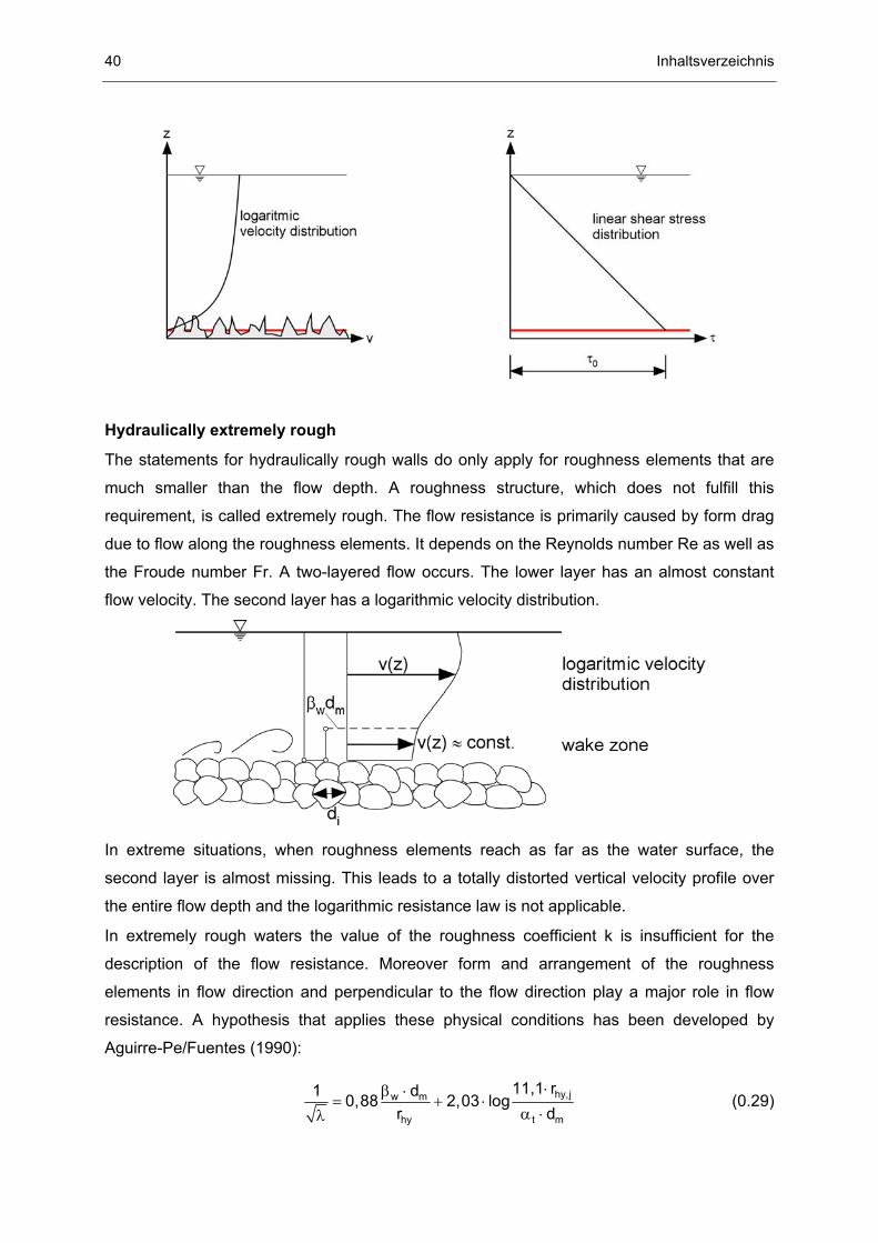
Hydraulically extremely rough
The statements for hydraulically rough walls do only apply for roughness elements that are
much smaller than the flow depth. A roughness structure, which does not fulfill this
requirement, is called extremely rough. The flow resistance is primarily caused by form drag
due to flow along the roughness elements. It depends on the Reynolds number Re as well as
the Froude number Fr. A two-layered flow occurs. The lower layer has an almost constant
flow velocity. The second layer has a logarithmic velocity distribution.
In extreme situations, when roughness elements reach as far as the water surface, the
second layer is almost missing. This leads to a totally distorted vertical velocity profile over
the entire flow depth and the logarithmic resistance law is not applicable.
In extremely rough waters the value of the roughness coefficient k is insufficient for the
description of the flow resistance. Moreover form and arrangement of the roughness
elements in flow direction and perpendicular to the flow direction play a major role in flow
resistance. A hypothesis that applies these physical conditions has been developed by
Aguirre-Pe/Fuentes (1990):
hy,jw m
hy t m
11,1 rd1 0,88 2,03 logr d
⋅β ⋅= + ⋅
α ⋅λ (0.29)
Inhaltsverzeichnis 41
In this formula dm stands for the mean diameter of the roughness elements, αt stands for the
texture parameter which considers the shape and the arrangement of the roughness
elements and βw stands for the wake-parameter.
This relation considers both aspects of the two-layered flow and consists of two terms. The
first term describes the layer close to the bed and the second one describes the zone near
the surface.
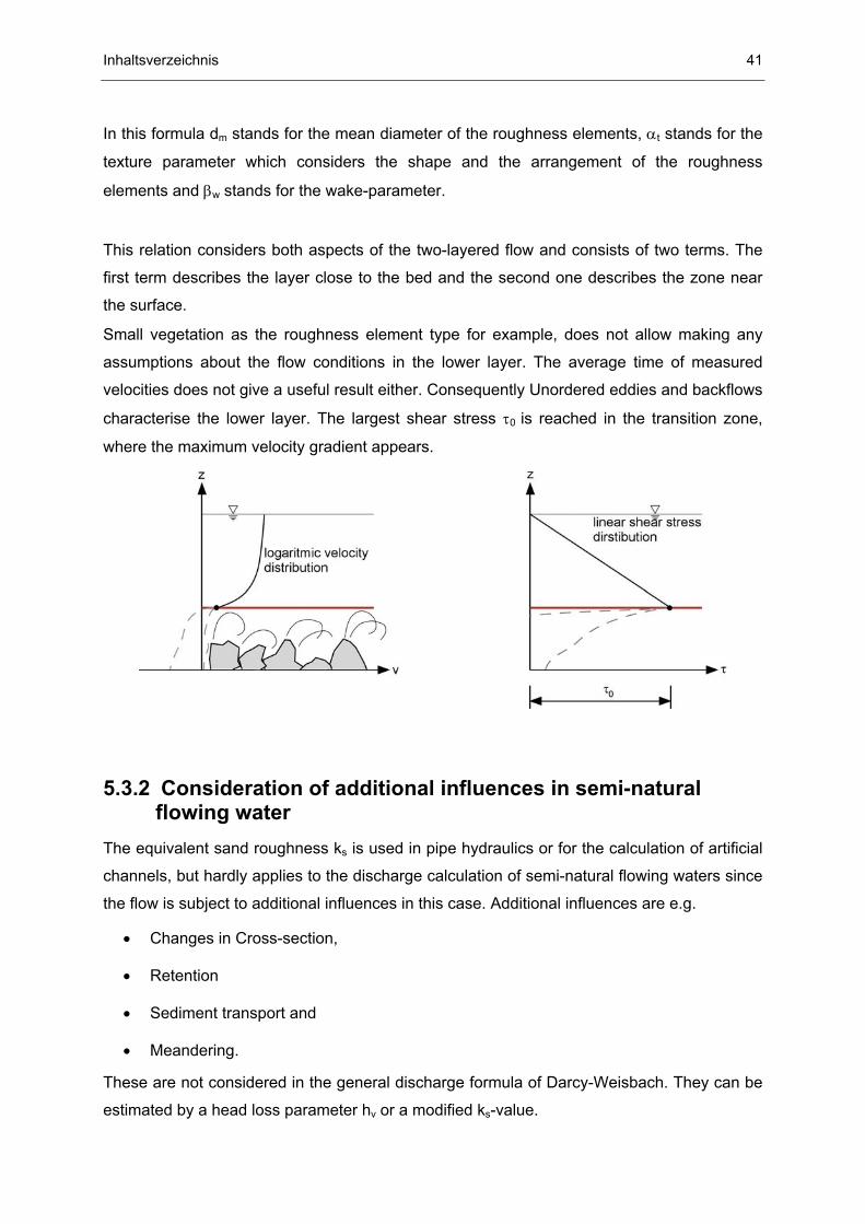
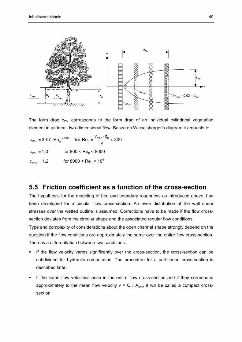
Small vegetation as the roughness element type for example, does not allow making any
assumptions about the flow conditions in the lower layer. The average time of measured
velocities does not give a useful result either. Consequently Unordered eddies and backflows
characterise the lower layer. The largest shear stress τ0 is reached in the transition zone,
where the maximum velocity gradient appears.
5.3.2 Consideration of additional influences in semi-natural flowing water
The equivalent sand roughness ks is used in pipe hydraulics or for the calculation of artificial
channels, but hardly applies to the discharge calculation of semi-natural flowing waters since
the flow is subject to additional influences in this case. Additional influences are e.g.
• Changes in Cross-section,
• Retention
• Sediment transport and
• Meandering.
These are not considered in the general discharge formula of Darcy-Weisbach. They can be
estimated by a head loss parameter hv or a modified ks-value.
42 Inhaltsverzeichnis
In the second case, modifications to the equivalent sand roughness (the so-called basic
roughness) ks have to be made. Only in case of small additional influences, the basic
roughness can be used for the calculations. A procedure for the determination of the
magnitude of additional parameters has not yet been developed. They are estimated by the
evaluation of measurements in nature. Analogical parameters can be used for flowing
waters, which have similar characteristics.
5.3.3 Meandering According to STEIN a simplified assumption was made in order to regard an additional flow
resistance. A friction coefficient, depending on the sinuosity of the stream, has been
developed. In order to get a correction factor for the total drag coefficient, it is made use of
the sinuosity:
λ = ⋅ λges,m m gesc (0.30)
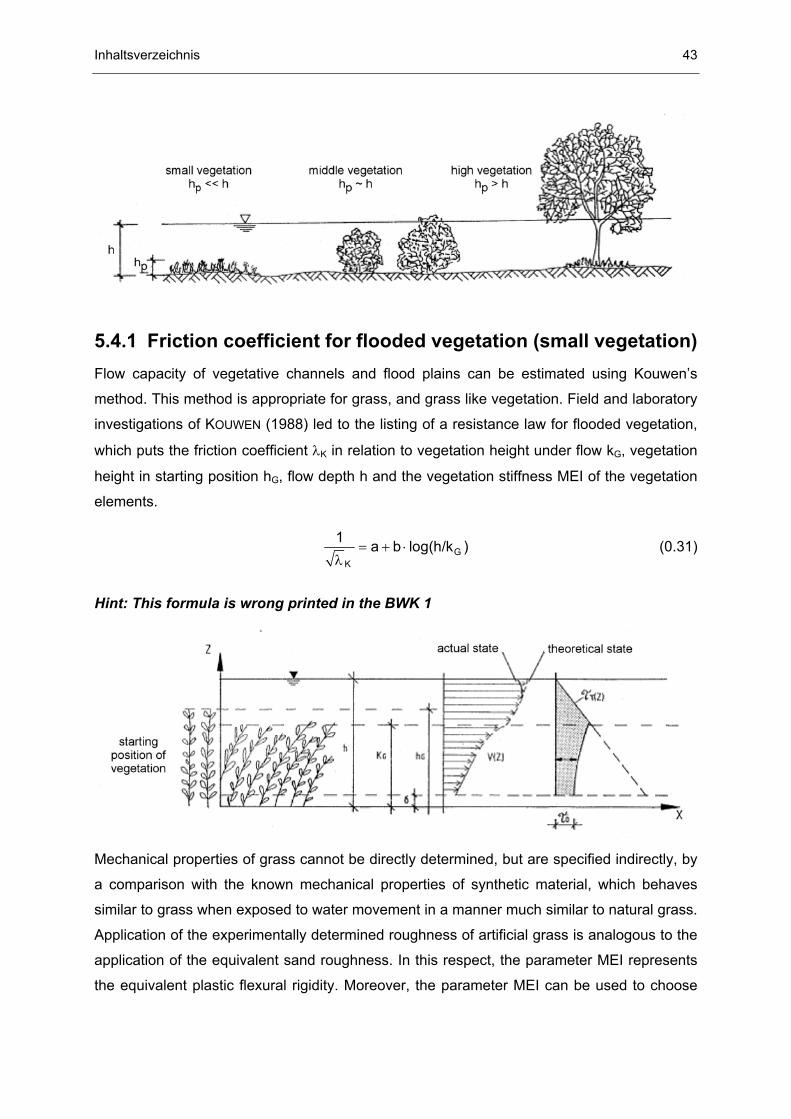
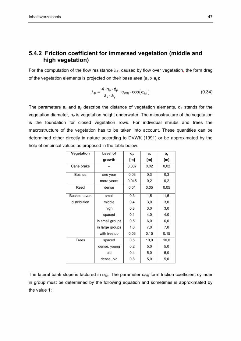
5.4 Friction coefficient for roughness caused by vegetation
For hydraulic quantification the vegetation of the banks and floodplains has to be classified. It
is differentiated between small, middle and high vegetation. If the vegetation height is
substantially smaller than the flow depth, the velocity distribution will turn out to be a
boundary layer flow. The flow is blocked by middle and high vegetation along the entire flow
depth. This loss caused by collision increases over the flow depth. Under these conditions
there is no logarithmic velocity distribution, moreover the flow velocity is constant along the
flow depth. For this reason small, middle and high vegetation must be described with
different approaches. According to this hydraulic effect a difference is made between flooded
(submerged), in-flow (immersed) and isolated vegetation.
Inhaltsverzeichnis 43
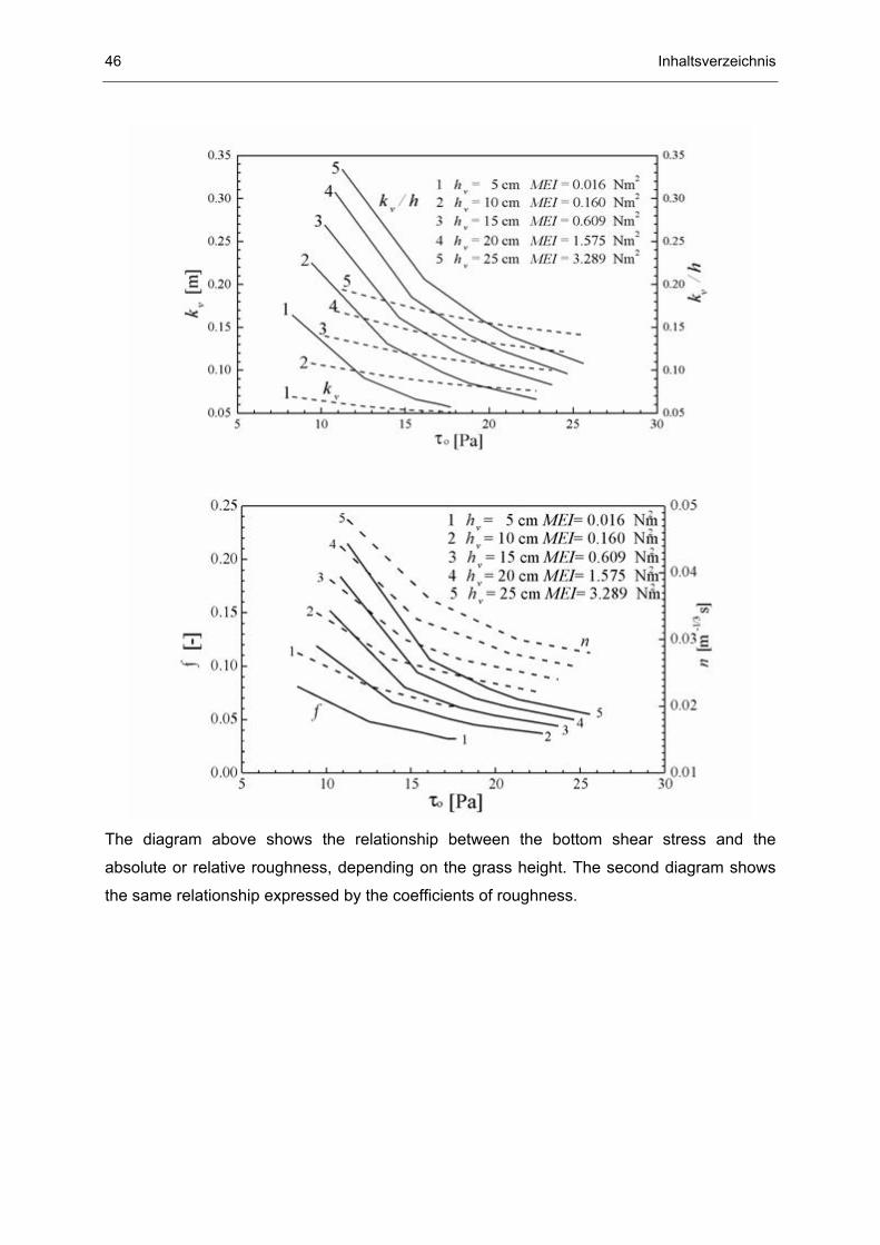
5.4.1 Friction coefficient for flooded vegetation (small vegetation) Flow capacity of vegetative channels and flood plains can be estimated using Kouwen’s
method. This method is appropriate for grass, and grass like vegetation. Field and laboratory
investigations of KOUWEN (1988) led to the listing of a resistance law for flooded vegetation,
which puts the friction coefficient λK in relation to vegetation height under flow kG, vegetation
height in starting position hG, flow depth h and the vegetation stiffness MEI of the vegetation
elements.
= + ⋅λ
GK
1 a b log(h/k ) (0.31)
Hint: This formula is wrong printed in the BWK 1
Mechanical properties of grass cannot be directly determined, but are specified indirectly, by
a comparison with the known mechanical properties of synthetic material, which behaves
similar to grass when exposed to water movement in a manner much similar to natural grass.
Application of the experimentally determined roughness of artificial grass is analogous to the
application of the equivalent sand roughness. In this respect, the parameter MEI represents
the equivalent plastic flexural rigidity. Moreover, the parameter MEI can be used to choose
44 Inhaltsverzeichnis
the most suitable types of grass for a particular design project (if climatologic or other factors
are not prevailing).
The parameters a and b are listed in the table. The vegetation height under flow is
approximated by the formula using the vegetation stiffness MEI:
1,590,25
SoG G
G
MEI
k 0,14 hh
τ = ⋅ ⋅
(0.32)
with: 3,3GMEI 319 h= ⋅ for grass
2,26GMEI 25,4 h= ⋅ for dead grass
So Eu
Aρ g Il
τ = ⋅ ⋅ ⋅ – shear stress at the bottom
The parameters a and b vary with the bending of the vegetation, which is expressed by the
relationship of the critical shear stress velocity v*krit to the actual shear stress velocity v*. With
the relationships
Ev* g h I= ⋅ ⋅ and krit 0,106
0,028 + 6,33 MEIv * Minimum von
0,23 MEI ⋅=
⋅ (0.33)
Bending parameter v*/v*
krit
Parameter a Parameter b
< 1,0 0,15 1,85
1,0 – 1,5 0,20 2,70
1,5 – 2,5 0,28 3,08
> 2,5 0,29 3,50
In opposition to the vegetation height hG the parameter MEI is not directly determinable in
nature. Kouwen (1990) therefore states the formulas for grass, so the parameter MEI can be
derived approximately from the grass height hG. For other flooded vegetations like shrubs
there are no empirical values for MEI. An exact but complex procedure for the direct
determination of MEI in the field is mentioned by Kouwen (1990).
Inhaltsverzeichnis 45
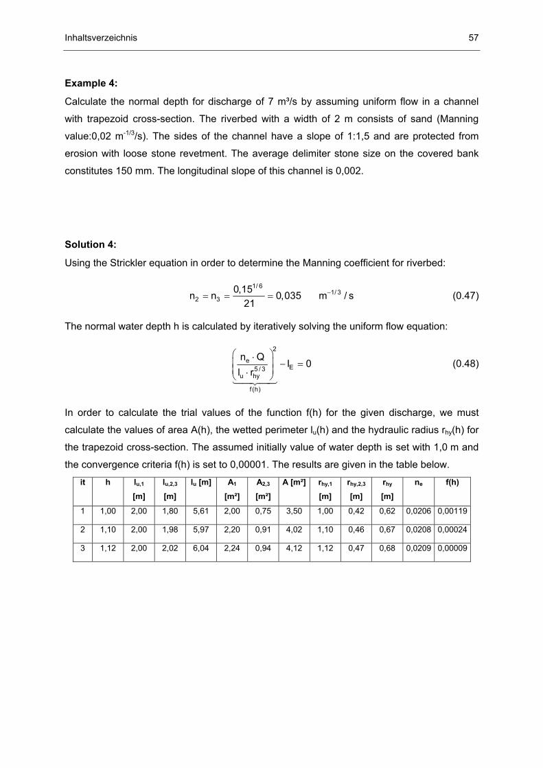
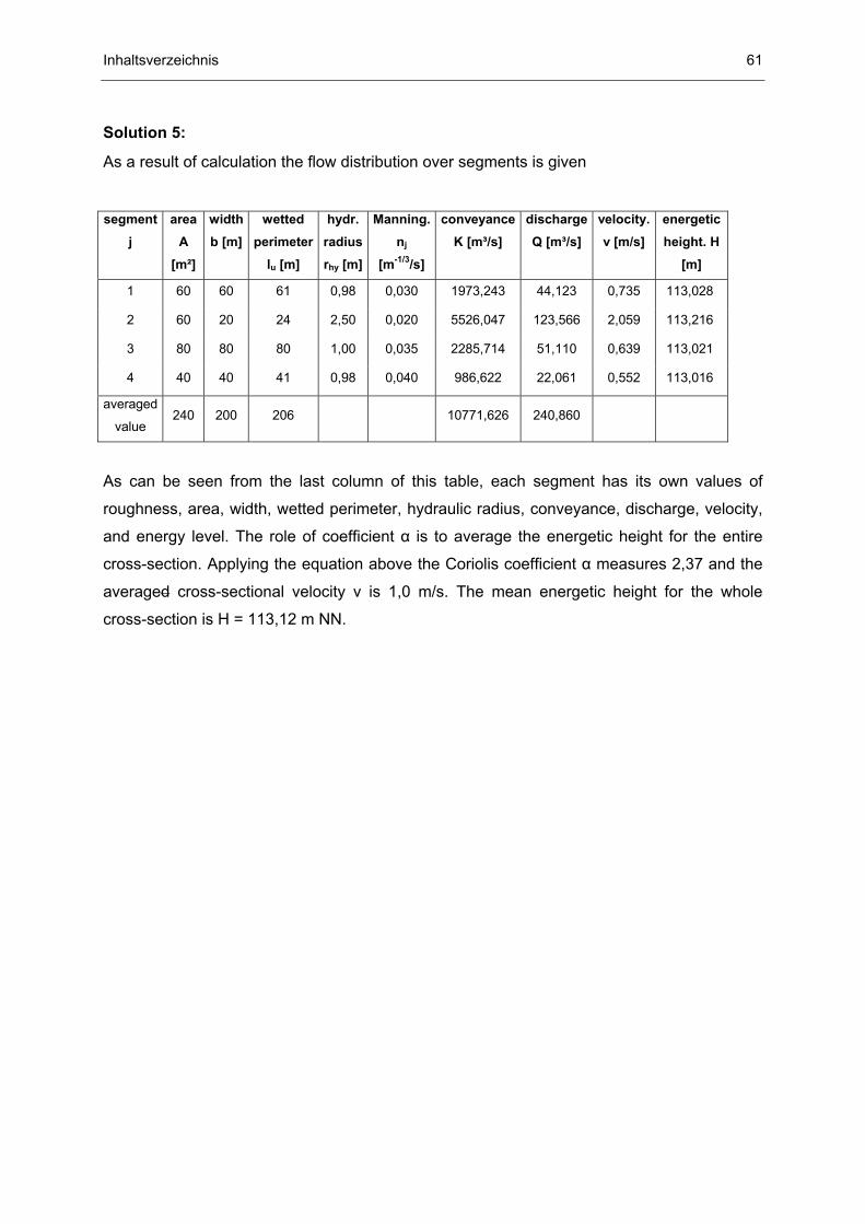
Example 3:
Determine the capacity of grass-lined channel of trapezoid cross-section, with a bottom width
of 5 m and a longitudinal bottom slope of 0,002. The average length of grass is 15 cm.
Assume steady, uniform flow conditions. The uniform flow equation should be solved
iteratively for some assumed discharge values: 2, 5, 8, 10 and 15 m³/s.
Solution 3:
Computing the values: MEI = 0,6094 Nm², v*= 0.218 m/s, and f
The results are presented in the table below. The sensitivity of parameters is also performed
and the results are shown.
Q [m³/s] h [m] A [m²] B [m] O [m] rhy [m] v [m/s] v* [m/s] kv [m] f [-] n [m1/3/s]
• Trapezoidal cross-sections with smooth boundary: ( )1/4hy Sof 1,13 r /b= ⋅
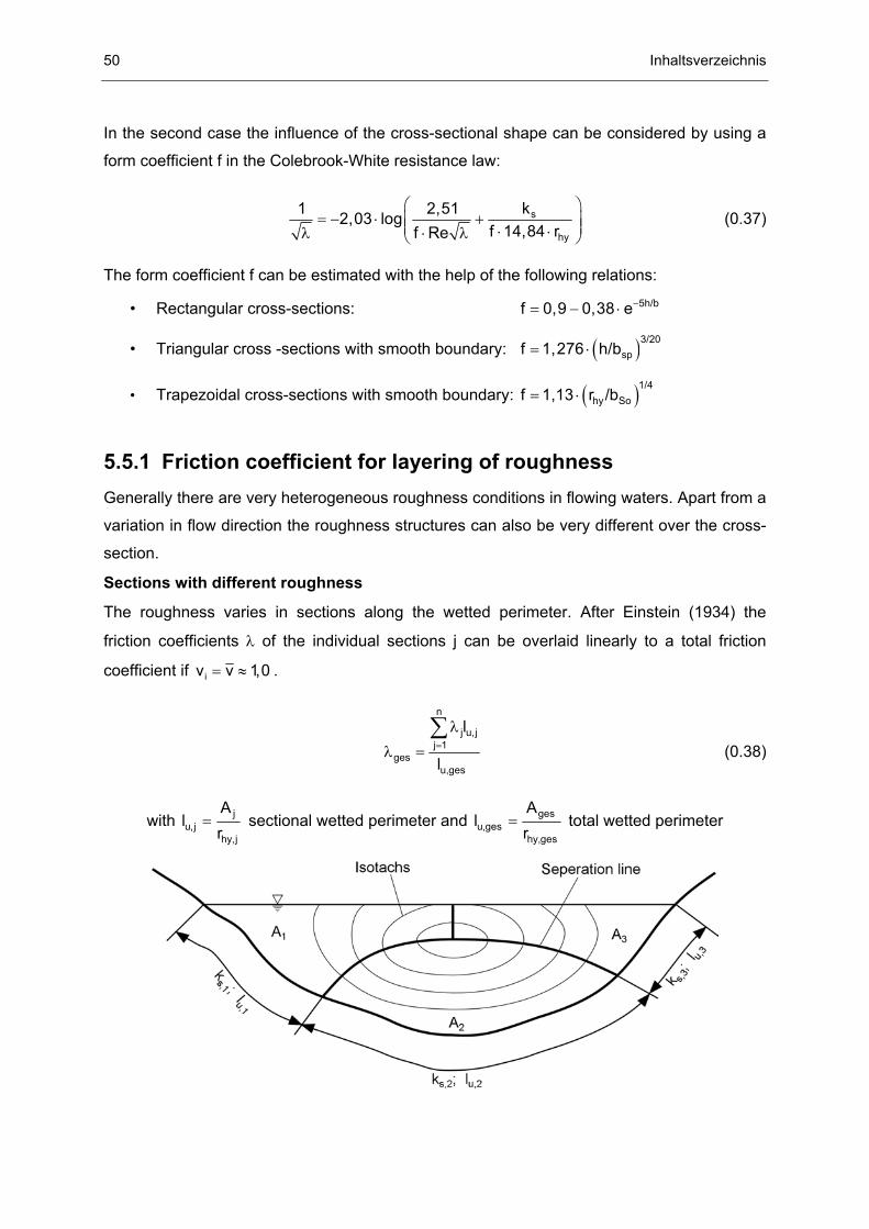
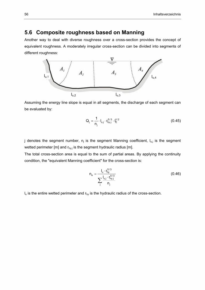
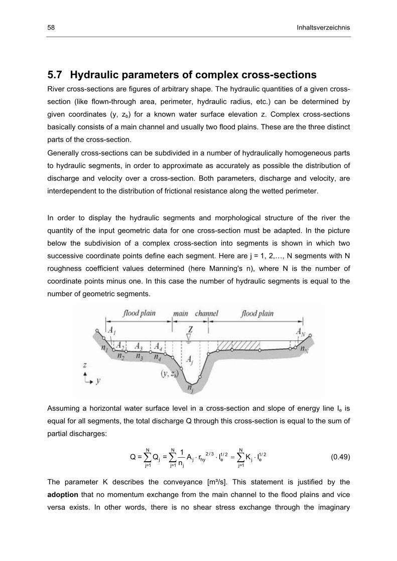
5.5.1 Friction coefficient for layering of roughness Generally there are very heterogeneous roughness conditions in flowing waters. Apart from a
variation in flow direction the roughness structures can also be very different over the cross-
section.
Sections with different roughness
The roughness varies in sections along the wetted perimeter. After Einstein (1934) the
friction coefficients λ of the individual sections j can be overlaid linearly to a total friction
coefficient if iv v 1,0= ≈ .
n
j u,jj 1
gesu,ges
l
l =
λ
λ =∑
(0.38)
with = ju,j
hy,j
Al
r sectional wetted perimeter and = ges
u,geshy,ges
Al
r total wetted perimeter
Inhaltsverzeichnis 51
Segments Aj are assigned to each of these sections. The size and the hydraulic radius of
these segments are proportional to the friction coefficient of the section:
j hy,j
ges hy,ges
rr
λ=
λ (0.39)
The friction coefficient λj is calculated by using the hydraulic radius of the segments rhy,j with
the Reynolds number Re:
s,j
hy,jj j
k1 2,512,03 log14,84 rRe
= − ⋅ + ⋅λ λ
with hy,jv 4 rRe
⋅ ⋅=
ν (0.40)
52 Inhaltsverzeichnis
Overlapping of roughness structures
According to Lindner (1982), the flow resistance caused by individual structures in smooth
and rough conditions can be overlaid linearly, if different roughness structures appear
together locally, e.g. submerged vegetation and immersed trees.
n
ges jj 1=
λ = λ∑ (0.41)
For extremely rough conditions the reliability of this method is not guaranteed. Since no flow
cross-sections can be assigned to vertically overlaying roughness classes, the friction
coefficient λj is calculated for the entire cross-section. In this case the hydraulic radius rhy,j of
the segment is not to be used in the Colebrook-White resistance law, but the hydraulic radius
of the cross-section rhy,ges in which the common roughness structures are located has to be
used.
5.5.2 Friction coefficient for partitioned cross-sections A partition of the flow cross-section is necessary whenever clear differences of local flow
velocities in the cross-section arise due to the cross-sectional shape or substantial
differences of bed roughness. Generally such conditions are:
• River-floodplain-flow and
• Flowing waters with vegetation on bank or floodplain
Inhaltsverzeichnis 53
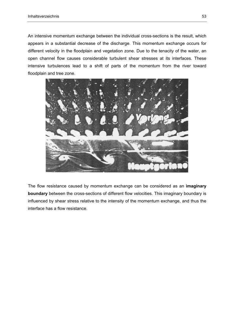
An intensive momentum exchange between the individual cross-sections is the result, which
appears in a substantial decrease of the discharge. This momentum exchange occurs for
different velocity in the floodplain and vegetation zone. Due to the tenacity of the water, an
open channel flow causes considerable turbulent shear stresses at its interfaces. These
intensive turbulences lead to a shift of parts of the momentum from the river toward
floodplain and tree zone.
The flow resistance caused by momentum exchange can be considered as an imaginary boundary between the cross-sections of different flow velocities. This imaginary boundary is
influenced by shear stress relative to the intensity of the momentum exchange, and thus the
interface has a flow resistance.
54 Inhaltsverzeichnis
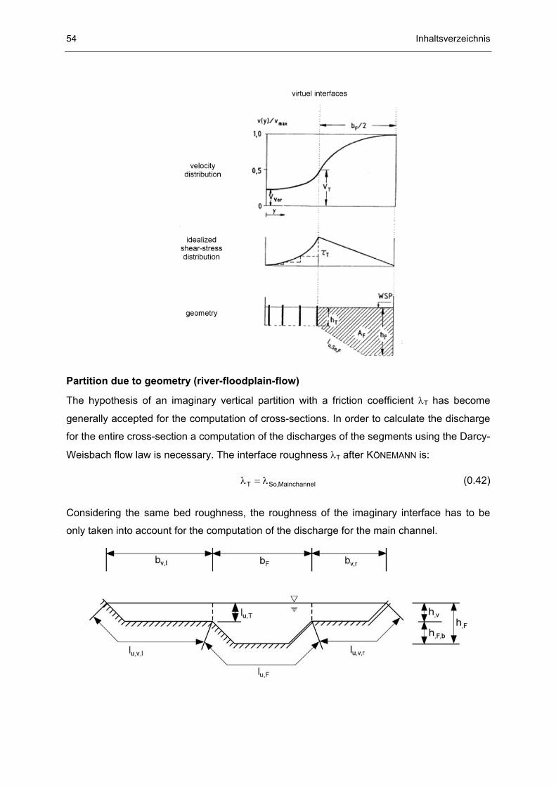
Partition due to geometry (river-floodplain-flow)
The hypothesis of an imaginary vertical partition with a friction coefficient λT has become
generally accepted for the computation of cross-sections. In order to calculate the discharge
for the entire cross-section a computation of the discharges of the segments using the Darcy-
Weisbach flow law is necessary. The interface roughness λT after KÖNEMANN is:
T So,Mainchannelλ = λ (0.42)
Considering the same bed roughness, the roughness of the imaginary interface has to be
only taken into account for the computation of the discharge for the main channel.
Inhaltsverzeichnis 55
Partition due to vegetation
The procedure after KÖNEMANN cannot be used if the bed roughness of the partitions differ
very much. If a partition of the cross-section due to vegetation is necessary, an imaginary
interface between vegetation zone and vegetation-free zone with a friction coefficient λT will
be assumed. The interface friction coefficient λT can be computed with the following formula:
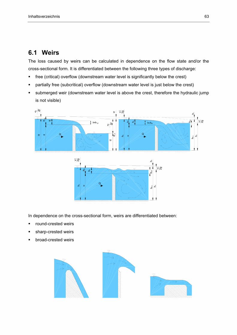
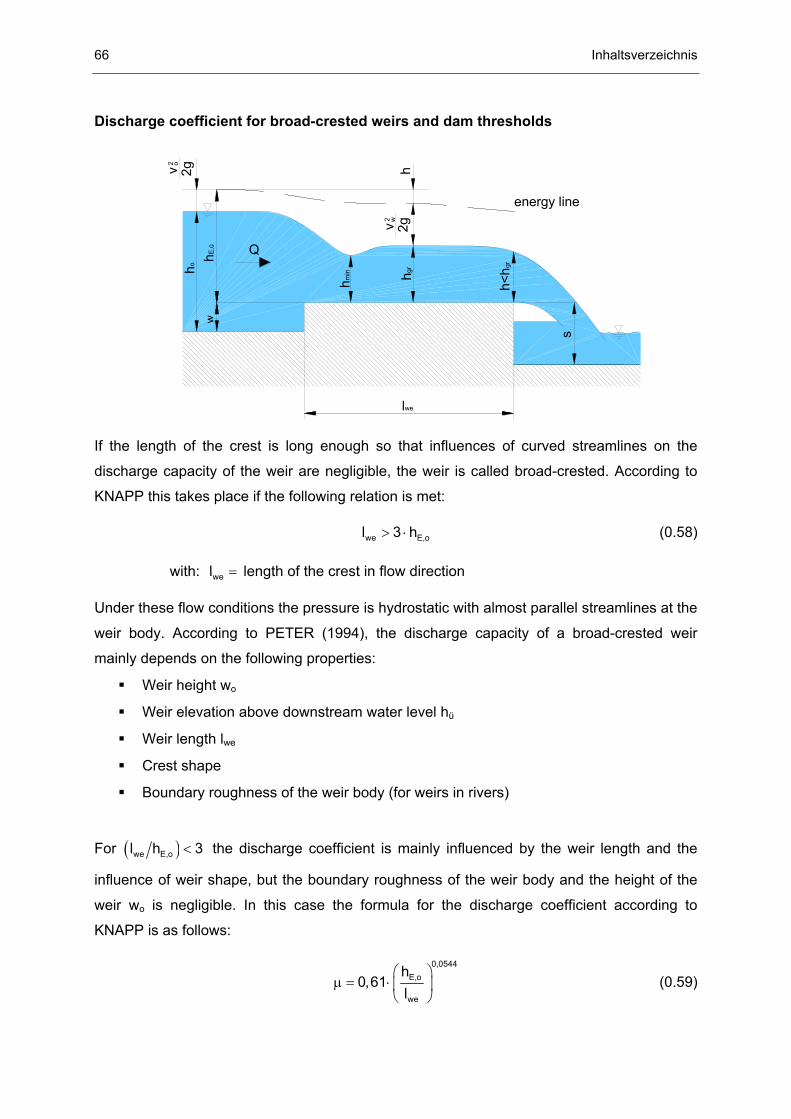
Discharge coefficient µ for different crest shapes of broad-crested weirs (from BWK 1999)
The diagram shows that for w = 0 there is no loss and the discharge coefficient has the
largest possible value: ( )1 3 0,577µ = .
68 Inhaltsverzeichnis
Discharge coefficient for dam-like weirs
The discharge capacity of weirs of this shape is approximately the same as the expected
discharge of a round-crested weir if the surface to the lower nappe is sufficiently aerated. It is
recommended to use the formula for round-crested weirs using hE,a for the upstream energy
head hE,o.
v2
w
hE,ü
hüo2
2gvenergy line
v1
6.1.2 Weirs with subcritical overflow The overflow is subcritical if the discharge is influenced by a respectively high downstream
water level huw. If the downstream water level rises the critical overflow becomes subcritical.
Then the discharge capacity and the loss at the weir do not only depend on the upstream
energy head hE,o but also on the downstream water level. There are boundary conditions for
round-crested weirs that define the transition between critical and subcritical overflow. For
broad-crested weirs the free overflow immediately becomes subcritical when the critical
depth at the downstream weir side is exceeded (KNAPP, 1969). An evaluation of momentum
conditions at the downstream weir side helps to describe this critical state mathematically. Boundary conditions for the different discharge states at weirs:
Discharge state
Weir shape
Submerged
flow
Free
overflow
Subcritical
overflow
Round-crested uw
gr
h 2,0h
≥ E,ouw
gr gr
hh 3,286 1,905h h
≤ − E,ouw
gr gr
hh2,0 3,286 1,905h h
≤ ≤ −
Broad-crested 2 22 2
uw u u u u
gr gr gr gr gr
h w v v w11 2h h g h g h h
≤ + + + − − ⋅
Inhaltsverzeichnis 69
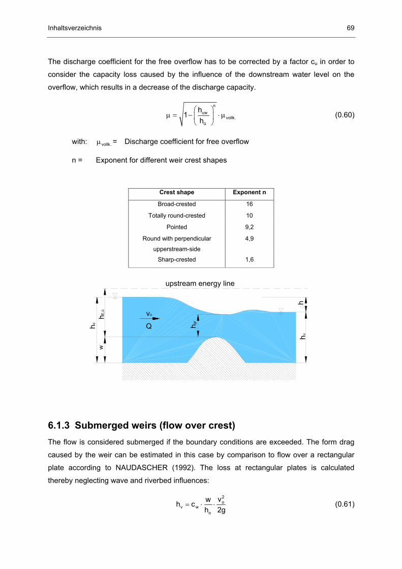
The discharge coefficient for the free overflow has to be corrected by a factor cu in order to
consider the capacity loss caused by the influence of the downstream water level on the
overflow, which results in a decrease of the discharge capacity.
µ = − ⋅ µ
nuw
vollk.ü
h1
h (0.60)
with: vollk.µ = Discharge coefficient for free overflow
n = Exponent for different weir crest shapes
Crest shape Exponent n
Broad-crested 16
Totally round-crested 10
Pointed 9,2
Round with perpendicular
upperstream-side
4,9
Sharp-crested 1,6
upstream energy line
w
vo
QhohE
,ü
hgr
hhu
6.1.3 Submerged weirs (flow over crest) The flow is considered submerged if the boundary conditions are exceeded. The form drag
caused by the weir can be estimated in this case by comparison to flow over a rectangular
plate according to NAUDASCHER (1992). The loss at rectangular plates is calculated
thereby neglecting wave and riverbed influences:
2o
v wo
vwh ch 2g
= ⋅ ⋅ (0.61)
70 Inhaltsverzeichnis
In the case of a sharp-crested weir body the form drag coefficient has the largest value of
wc 1,9= according to NAUDASCHER (1992). It is lower if the weir shape is more
streamlined.
6.1.4 Weirs with different crest heights If the weir crest differs in height, the weir body has to be partitioned into sections of equal
height. Assuming a constant energy height E,oh the partial discharge jq and the discharge
coefficient jµ have to be calculated for each section.
3 2j j E,o
2q 2g h3
= ⋅ ⋅ µ ⋅ (0.62)
The energy height E,oh as well as the partial discharges jq are unknown. Due to the implicit
linking of the partial discharges with the energy height E,oh the calculation can be done in
iterations varying E,oh until the total discharge is equal to the real discharge.
( )n
ges j w,jj 1
Q q b=
= ⋅∑ (0.63)
with: n = number of weir sections with constant height
w,jb = width of section j
Inhaltsverzeichnis 71
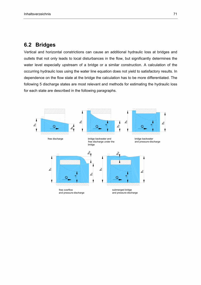
6.2 Bridges Vertical and horizontal constrictions can cause an additional hydraulic loss at bridges and
outlets that not only leads to local disturbances in the flow, but significantly determines the
water level especially upstream of a bridge or a similar construction. A calculation of the
occurring hydraulic loss using the water line equation does not yield to satisfactory results. In
dependence on the flow state at the bridge the calculation has to be more differentiated. The
following 5 discharge states are most relevant and methods for estimating the hydraulic loss
for each state are described in the following paragraphs.
bridge backwater andfree discharge under the bridge
72 Inhaltsverzeichnis
6.2.1 Free discharge at a bridge The discharge is free if the water levels upstream as well as downstream of the bridge are
below the lower edge of the bridge. Horizontal narrowing due to bearings, access ramps or
piers can cause flow resistance. By the Rehbock pier-formula the flow resistance of a pier
can be calculated differentiating between a compact cross-section with an almost even flow
velocity and a structured cross-section with an uneven velocity distribution. The Rehbock pier
formula can also be used to calculate the loss as a result of side-constructions (based on
model experiments by SCHWARZE (1969)). The calculated backwater has to be multiplied
by a correctional factor.
Rehbockh c h∆ = ⋅ ∆ (0.64)
The coefficient c takes the following values depending on the channel shape:
River bed geometry c Valid range
Rectangular Verb0,4 2,45 A / A+ ⋅
Verb uA / A 0,24≤
2 Verb u0,2 2,33 A / A+ ⋅
Verb uA / A 0,34≤ Trapezoidal
Bank
Slope [m]
3 Verb u0,28 A / A⋅ Verb uA / A 0,44≤
For structured cross-sections with an uneven velocity distribution SCHWARZE (1969)
suggested to correct the pier backwater by a factor, similar to horizontal contractions.
Rehbockh c h∆ = ⋅ ∆ (0.65)
The correctional factor is computed with pf,j pf,j jA d h= ⋅ = obstructed cross-section,
gesA v Q⋅ = , jv = velocity upstream of the bridge and the obstructed section j. With pfl = pier
length in flow direction and pfd = pier width.
Inhaltsverzeichnis 73
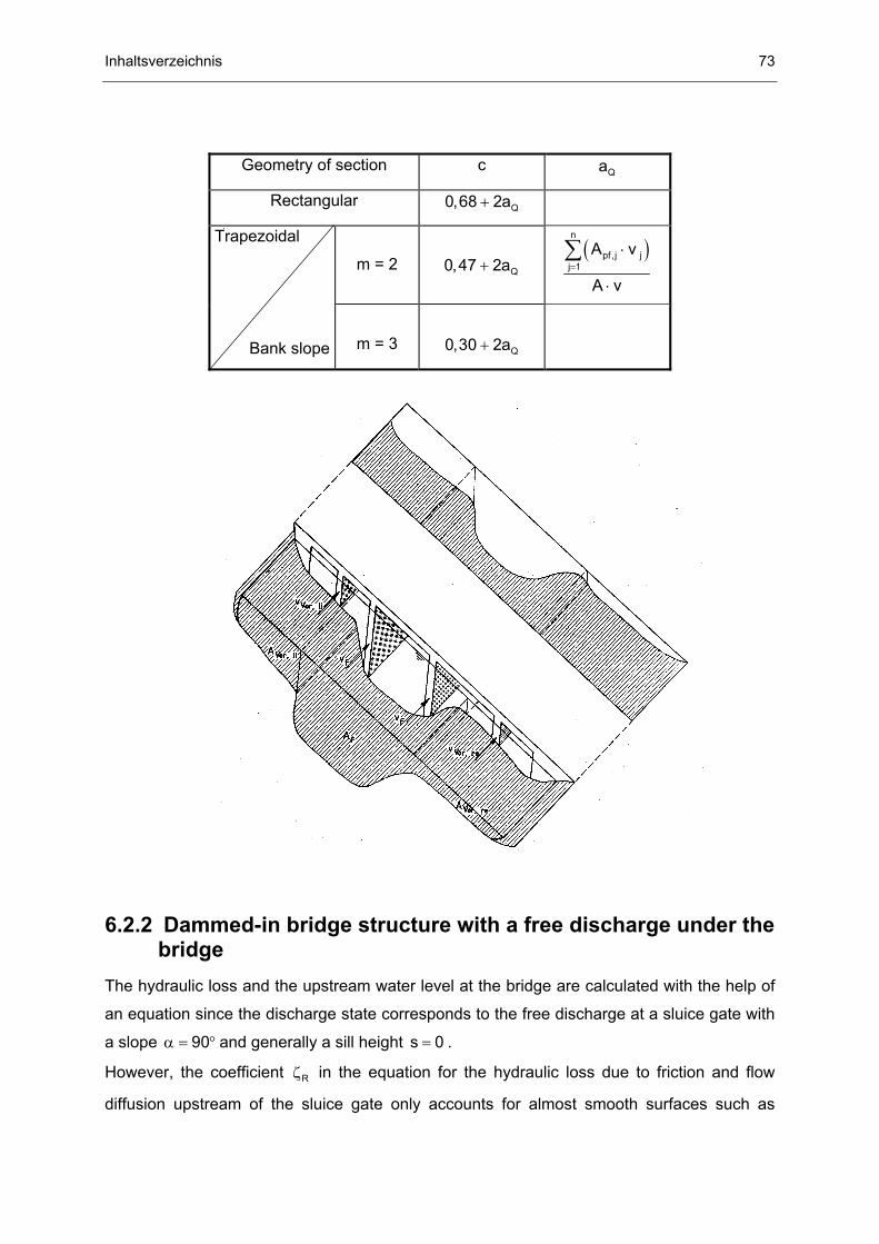
Geometry of section c Qa
Rectangular Q0,68 2a+
m = 2
Q0,47 2a+ ( )
n
pf,j jj 1
A v
A v=
⋅
⋅
∑
Trapezoidal
Bank slope
m = 3
Q0,30 2a+
6.2.2 Dammed-in bridge structure with a free discharge under the bridge
The hydraulic loss and the upstream water level at the bridge are calculated with the help of
an equation since the discharge state corresponds to the free discharge at a sluice gate with
a slope 90α = ° and generally a sill height s 0= .
However, the coefficient Rζ in the equation for the hydraulic loss due to friction and flow
diffusion upstream of the sluice gate only accounts for almost smooth surfaces such as
74 Inhaltsverzeichnis
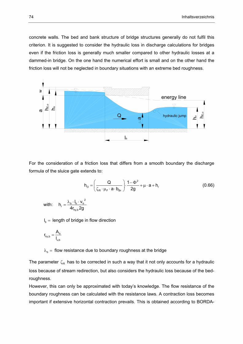
concrete walls. The bed and bank structure of bridge structures generally do not fulfil this
criterion. It is suggested to consider the hydraulic loss in discharge calculations for bridges
even if the friction loss is generally much smaller compared to other hydraulic losses at a
dammed-in bridge. On the one hand the numerical effort is small and on the other hand the
friction loss will not be neglected in boundary situations with an extreme bed roughness.
energy line
wa
a
ho
Q
lb
huhydraulic jump hE,u
hE,o
For the consideration of a friction loss that differs from a smooth boundary the discharge
formula of the sluice gate extends to:
2
O rR F Br
Q 1h a ha b 2g
− Φ= ⋅ + µ ⋅ + ζ ⋅ µ ⋅ ⋅
(0.66)
with: 2
b b br
hy,b
l vh4r 2g
λ ⋅ ⋅=
bl = length of bridge in flow direction
bhy,b
u,b
Arl
=
bλ = flow resistance due to boundary roughness at the bridge
The parameter Rζ has to be corrected in such a way that it not only accounts for a hydraulic
loss because of stream redirection, but also considers the hydraulic loss because of the bed-
roughness.
However, this can only be approximated with today’s knowledge. The flow resistance of the
boundary roughness can be calculated with the resistance laws. A contraction loss becomes
important if extensive horizontal contraction prevails. This is obtained according to BORDA-
Inhaltsverzeichnis 75
CARNOT. It leads to an extension of the equation by the loss head Verbauh that is calculated
as follows:
2 2u u
Verbau u Ov vh2g 2g
= ζ ⋅ + ζ ⋅ (0.67)
with: 2
bu a
u
Ac 1A
ζ = −
and
2
oo e
b
Ac 1A
ζ = −
6.2.3 Dammed-in bridge structure with backwater (subcritical discharge)
The hydraulic loss that has to be considered is obtained in analogy to the discharge at a
sluice gate with subcritical discharge since the two discharge situations are almost equal. For
the consideration of a higher friction loss and hydraulic loss due to horizontal contraction the
equation above has to be extended by the loss heads Rh∆ and Verbauh∆ .
In general the bed at bridges is even so that the hydraulic loss of a sill below the water
surface can be neglected and the equations for the parameters m and n become much
simpler since the sill height is set to s=0 and 0ε = .
6.2.4 Submerged bridge structure with supercritical flow The prevalent discharge situation can be divided into two components. On the one hand the
stream still discharges through the bridge (pressure discharge) and on the other hand there
is a part that is discharged according to a weir over the bridge deck. The first case mostly
corresponds to the case of a sluice gate with submerged flow. This means the discharge
through the bridge can be determined without taking care of the discharge over the bridge.
76 Inhaltsverzeichnis
energy line
wa
a
hE,o
hühb
ok
Q
lb
2gv u2
hvhu
hmin
hgr h<hgr
The relative crest height ( )E,o bok bh h l 3,0− < generally fits the spill situation at the bridge.
Since this spill situation corresponds to a broad-crested weir, the discharge part over the
bridge can be calculated with the DU BUAT equation:
( )3 / 2ü b E,o bok
2Q b 2g h h3
= µ ⋅ ⋅ − (0.68)
with the discharge coefficient µ:
0,0544
E,o bok
b
h h0,61
l−
µ = ⋅
(0.69)
Even if the spill situation mostly corresponds to a broad-crested weir, the discharge
coefficients (occurring for stream-lined flow edges) cannot be assumed accurately since for
both upstream and downstream the bridge deck is generally sharp-edged.
Since the discharge partition of submerged and subcritical parts of the bridge depends on the
energy head upstream of the bridge and the total discharge, the discharge partition has to be
found iteratively. The right partition is found when the continuity equation is met as an
additional boundary condition:
ges D ÜQ Q Q= + (0.70)
with: DQ = discharge under the bridge
ÜQ = discharge over the bridge
Inhaltsverzeichnis 77
Depending on the discharge state, QD has to be obtained as follows:
For free (critical) discharge: with equation (0.15) solved for Q
For subcritical discharge: D R F sHQ a b 2g
1∆
= ρ ⋅ µ ⋅ ⋅− Φ
(0.71)
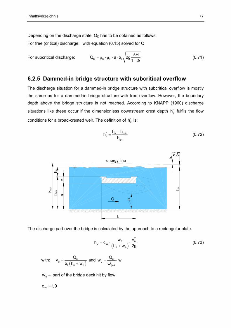
6.2.5 Dammed-in bridge structure with subcritical overflow The discharge situation for a dammed-in bridge structure with subcritical overflow is mostly
the same as for a dammed-in bridge structure with free overflow. However, the boundary
depth above the bridge structure is not reached. According to KNAPP (1960) discharge
situations like these occur if the dimensionless downstream crest depth uh∗ fulfils the flow
conditions for a broad-crested weir. The definition of uh∗ is:
* u boku
gr
h hhh−
= (0.72)
energy line
wa
a
hE,o
hühb
ok
Q
lb
2gv u2hv
hu
The discharge part over the bridge is calculated by the approach to a rectangular plate.
( )
2ü ü
V Wü ü
w vh ch w 2g
= ⋅ ⋅+
(0.73)
with: ( )
üü
b ü ü
Qvb h w
=+
and üü
ges
Qw wQ
= ⋅
üw = part of the bridge deck hit by flow
Wc 1,9=
78 Inhaltsverzeichnis
Due to the implicit connection of the parameters in these equations the discharge partition of
DQ and ÜQ has to be determined iteratively. The right discharge partition is found if the
continuity equation is reached on the one side and the energy head E,oh upstream of the
bridge is equal to the energy head used in the calculation of the partial discharge ÜQ over
the bridge structure on the other side of the equation.
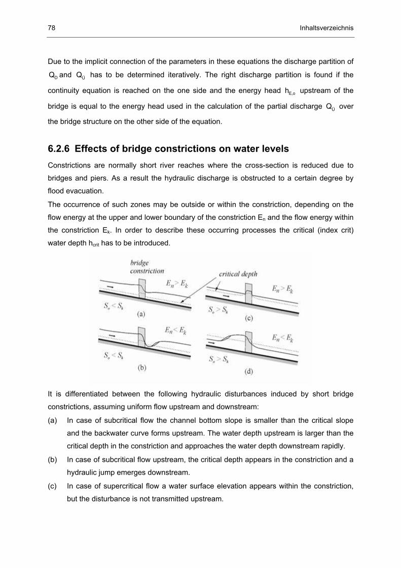
6.2.6 Effects of bridge constrictions on water levels Constrictions are normally short river reaches where the cross-section is reduced due to
bridges and piers. As a result the hydraulic discharge is obstructed to a certain degree by
flood evacuation.
The occurrence of such zones may be outside or within the constriction, depending on the
flow energy at the upper and lower boundary of the constriction En and the flow energy within
the constriction Ek. In order to describe these occurring processes the critical (index crit)
water depth hcrit has to be introduced.
It is differentiated between the following hydraulic disturbances induced by short bridge
constrictions, assuming uniform flow upstream and downstream:
(a) In case of subcritical flow the channel bottom slope is smaller than the critical slope
and the backwater curve forms upstream. The water depth upstream is larger than the
critical depth in the constriction and approaches the water depth downstream rapidly.
(b) In case of subcritical flow upstream, the critical depth appears in the constriction and a
hydraulic jump emerges downstream.
(c) In case of supercritical flow a water surface elevation appears within the constriction,
but the disturbance is not transmitted upstream.
Inhaltsverzeichnis 79
(d) In case of a great constriction, so that En < Ek, a hydraulic jump occurs upstream,
shortly before the constriction.
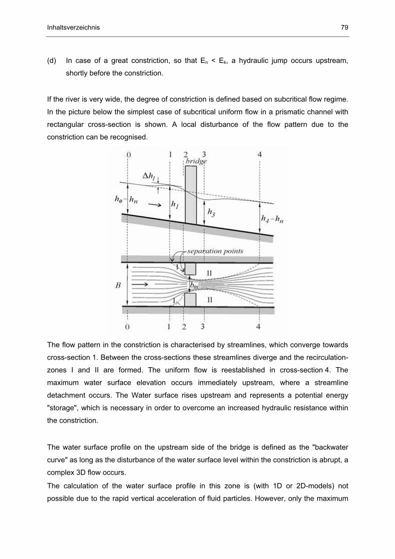
If the river is very wide, the degree of constriction is defined based on subcritical flow regime.
In the picture below the simplest case of subcritical uniform flow in a prismatic channel with
rectangular cross-section is shown. A local disturbance of the flow pattern due to the
constriction can be recognised.
The flow pattern in the constriction is characterised by streamlines, which converge towards
cross-section 1. Between the cross-sections these streamlines diverge and the recirculation-
zones I and II are formed. The uniform flow is reestablished in cross-section 4. The
maximum water surface elevation occurs immediately upstream, where a streamline
detachment occurs. The Water surface rises upstream and represents a potential energy
"storage", which is necessary in order to overcome an increased hydraulic resistance within
the constriction.
The water surface profile on the upstream side of the bridge is defined as the "backwater
curve" as long as the disturbance of the water surface level within the constriction is abrupt, a
complex 3D flow occurs.
The calculation of the water surface profile in this zone is (with 1D or 2D-models) not
possible due to the rapid vertical acceleration of fluid particles. However, only the maximum
80 Inhaltsverzeichnis
water surface increase (delta h = h1-h2) is needed for engineering purposes. This rise is
easily calculated with mass and energy conservation laws, applied for cross-sections with
parallel streamlines and the pressure distribution is hydrostatic (cross-sections 1, 3 and 4).
Energy losses due to friction can be neglected because these sections are so close to each
other that only local energy losses due to abrupt changes of geometry must to be taken into
account.
Inhaltsverzeichnis 81
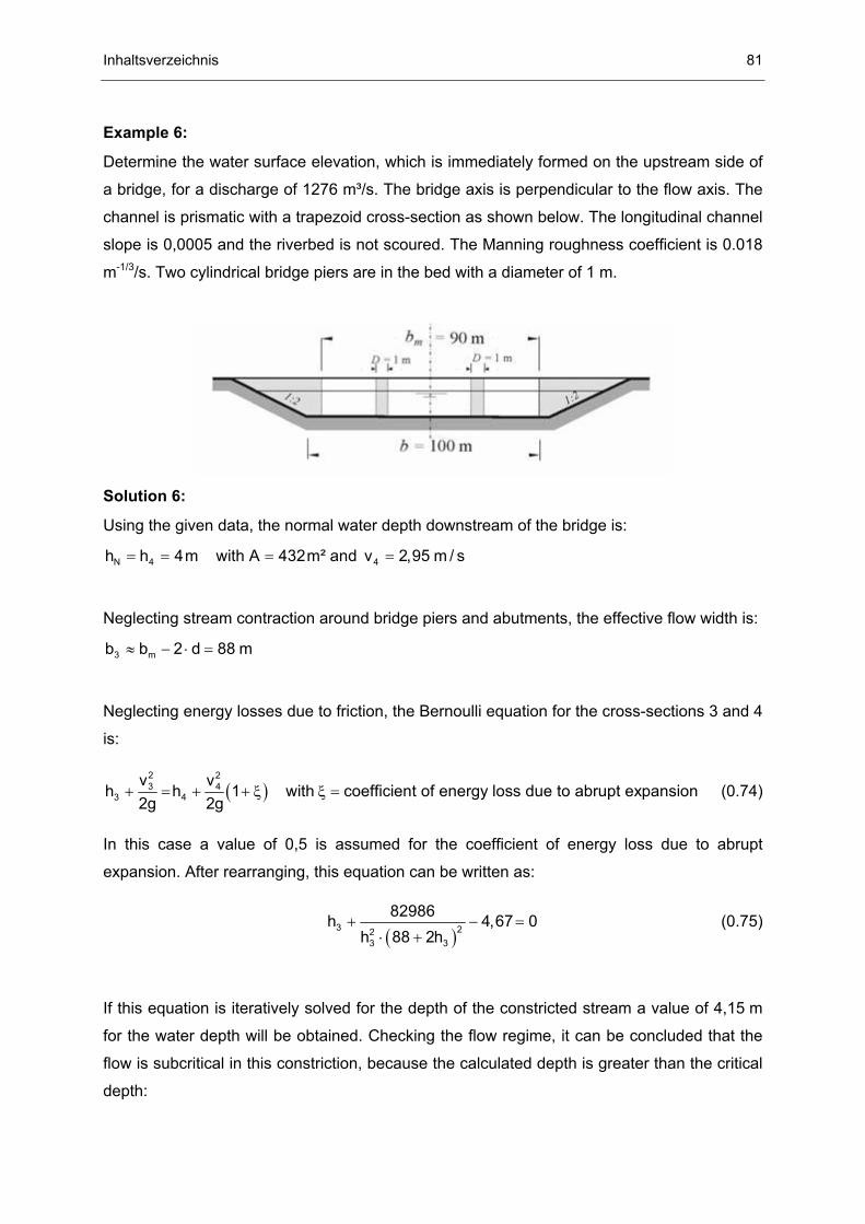
Example 6:
Determine the water surface elevation, which is immediately formed on the upstream side of
a bridge, for a discharge of 1276 m³/s. The bridge axis is perpendicular to the flow axis. The
channel is prismatic with a trapezoid cross-section as shown below. The longitudinal channel
slope is 0,0005 and the riverbed is not scoured. The Manning roughness coefficient is 0.018
m-1/3/s. Two cylindrical bridge piers are in the bed with a diameter of 1 m.
Solution 6:
Using the given data, the normal water depth downstream of the bridge is:
= = = =N 4 4h h 4m with A 432m² and v 2,95 m / s
Neglecting stream contraction around bridge piers and abutments, the effective flow width is:
≈ − ⋅ =3 mb b 2 d 88 m
Neglecting energy losses due to friction, the Bernoulli equation for the cross-sections 3 and 4
is:
( )+ = + + ξ ξ =2 23 4
3 4v v
h h 1 with coefficient of energy loss due to abrupt expansion2g 2g
(0.74)
In this case a value of 0,5 is assumed for the coefficient of energy loss due to abrupt
expansion. After rearranging, this equation can be written as:
( )
+ − =⋅ +
3 223 3
82986h 4,67 0h 88 2h
(0.75)
If this equation is iteratively solved for the depth of the constricted stream a value of 4,15 m
for the water depth will be obtained. Checking the flow regime, it can be concluded that the
flow is subcritical in this constriction, because the calculated depth is greater than the critical
depth:
82 Inhaltsverzeichnis
( ) = = =
1/ 321/ 32 127688
critqh 2,78 mg 9,81
The Bernoulli equation for the cross-sections 1 and 3 is:
( )+ = + + ξ ξ =2231
1 3 c cvv
h h 1 with coefficient of energy loss due to abrupt constriction2g 2g
(0.76)
In this case a value of 0,3 is assumed for the coefficient of energy loss due to abrupt
constriction. After rearranging:
( )
+ − =⋅ +
1 221 1
82986h 4,82 0h 90 2h
(0.77)
By solving this equation iteratively, an upstream depth of 4,40 m is determined. Thus, the
water surface elevation due to the bridge constriction is 0,40 m.
Inhaltsverzeichnis 83
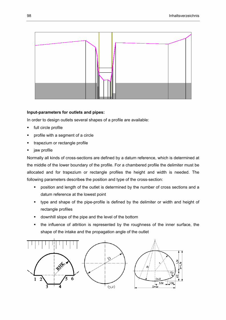
6.3 Pipes and outlets As in local gorge portions for outlets an additional loss of hydraulic energy must be included
in order to solve the shallow-water-equation. The loss of hydraulic energy at the entrance,
caused by discharge and friction is displayed by coefficients.
6.3.1 Attrition of hydraulic energy The influence of attrition of hydraulic energy is important for the computation of the water
shallow equation. Basically it is distinguished between continuous and local losses. For
example the roughness of a pipe does only include the friction on the path, but no local
variations. These local attritions are shown by a universal approach. The coefficient of
attrition depends on the type and form of the imperfection:
−= ζ ⋅2i 1
ZV Vv
H2g
(0.78)
The loss of hydraulic energy caused at the entrance depends on the design of intake areas.
It is subdivided between the following formations:
The loss of hydraulic energy increases as the flow velocity in the pipe accelerates. If the
outlet is very short the main loss is caused by the intake.
The loss of hydraulic energy caused by the roughness of the pipe, which depends on the
material of the inner surface, is calculated by using the friction equation of PRANDTL-
COLEBROOK in combination with the flow formula of MANNING-STRICKLER. If the length of an
outlet is ten-times bigger than the delimiter, the application of the equation of PRANDTL-
COLEBROOK is recommended. The roughness of a pipe can vary in a cross section or over
the path.
84 Inhaltsverzeichnis
In order to determine the loss of hydraulic energy caused by discharge units the equation of
BORDA-CARNOT is applied. For conic expansions at the outlet the following reduction-factor ca
as a function of the propagation angle is used:
The reduction-factor ca is used to calculate the height of attrition, which is based on
expansions, with the following equation form BORDA- CARNOT:
−− = ⋅
2i i 1
ZV av v
H c2g
(0.79)
The Terms vi and vi-1 describe the averaged values of velocity.
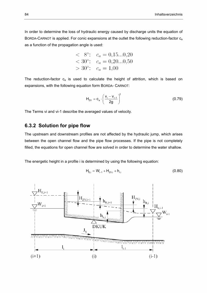
6.3.2 Solution for pipe flow The upstream and downstream profiles are not affected by the hydraulic jump, which arises
between the open channel flow and the pipe flow processes. If the pipe is not completely
filled, the equations for open channel flow are solved in order to determine the water shallow.
The energetic height in a profile i is determined by using the following equation:
−= + +E,i i 1 ZV,i r,iH W H h (0.80)
Inhaltsverzeichnis 85
The slope of the friction is approximated by a water level at the beginning or the height of the
pressure level in the profile i. Likewise the energetic height is approximated by a water level
at the beginning of profile i. If outlets or pipes are completely filled the energetic height
consists of the level of pressure and the height, which describes the kinematical energy
caused by velocity.
This height of kinematical energy results from the known discharge and the flow-through-
area of the profile.
= ⋅⋅
2 2i
k,i 2i
v Qh2g A 2g
(0.81)
86 Inhaltsverzeichnis
7 Retention
Retention describes the time lag of water run-off processes as a phenomenon of natural
rivers. This effect considers the deformation of a flood wave in a watercourse and on flood
plains. It is distinguished between stagnant and flowing retention or natural and artificial
retention. All these phenomena result in a deformation of the discharge-time graph, the so-
called hydrograph. In order to compute the form of outflow hydrograph the deformation must
be described mathematically. Retention and deformation of the hydrograph:
Inhaltsverzeichnis 87
Flowing Retention in the watercourse
The flow process in a watercourse is affected by a loss of energy over the path. This loss of
energy influences the retention, which depends on slope, discharge and bed material and its
distribution over the cross section. Together with the bed material, which is disclosed in
roughness classes, the vegetation of a watercourse or on the flood plain influences the
retention in the channel. Additionally the longitudinal profile of a river and its variety of
morphological structures affect this phenomenon. If a river is meandered and includes
branches, islands, banks and scours the retention of flood peaks decreases.
If the bank-full discharge is over topped, the interaction due to the jump of friction between
foreland and riverbed decelerates the velocity in the watercourse. The interaction is caused
by momentum exchange between the cross-sections of different flow velocities.
Flowing Retention on flood plains
Normally the roughness of a flood plain increases and the vegetation is denser than in the
channel. If the flood plain is inundated the width of the water shallow increases faster than
the water depth and the retention can be compared to the effects, which occur in a
compound channel. Due to a lower water depth and a higher friction the water in flood plains
flows more slowly. The retention on the flood plain is influenced by vegetation and the
existence of alluvial meadows, alluvial forests and bayous. If the flood plain is unspoilt and
open to get inundated during a flood event, normally a strong retention effect appears.
Stagnant Retention on flood plains and storage basin
If floodwater on the foreland is filling a bayou or a desiccated pond, a so-called stagnant
retention, appears. But even if the flow velocity decreases, the water remains on the
floodplain, this effect is reached and the flood peak is deformed.
This natural effect is used for artificially made retention basins. The constructions such as
polders, retention ponds and reservoirs are initiated to hold back the water in order to
decrease the flood discharge. A wise regulation of these measurements is essential for an
optimal flood management.
88 Inhaltsverzeichnis
8 Simulation with Kalypso 1D
Regarding a quite homogeneous natural river a one-dimensional simulation is effective and a
fast method to compute an averaged water depth and velocity. In this case homogeneity also
includes composed cross-section with vegetation, a slightly meandered river with hydraulic
structures in the channel and bifurcations. Only secondary flow processes such as
turbulence and superelevations of the water level in a cross-section as a result of a strong
meandered flow etc., should be examined in a 2D-simulation.
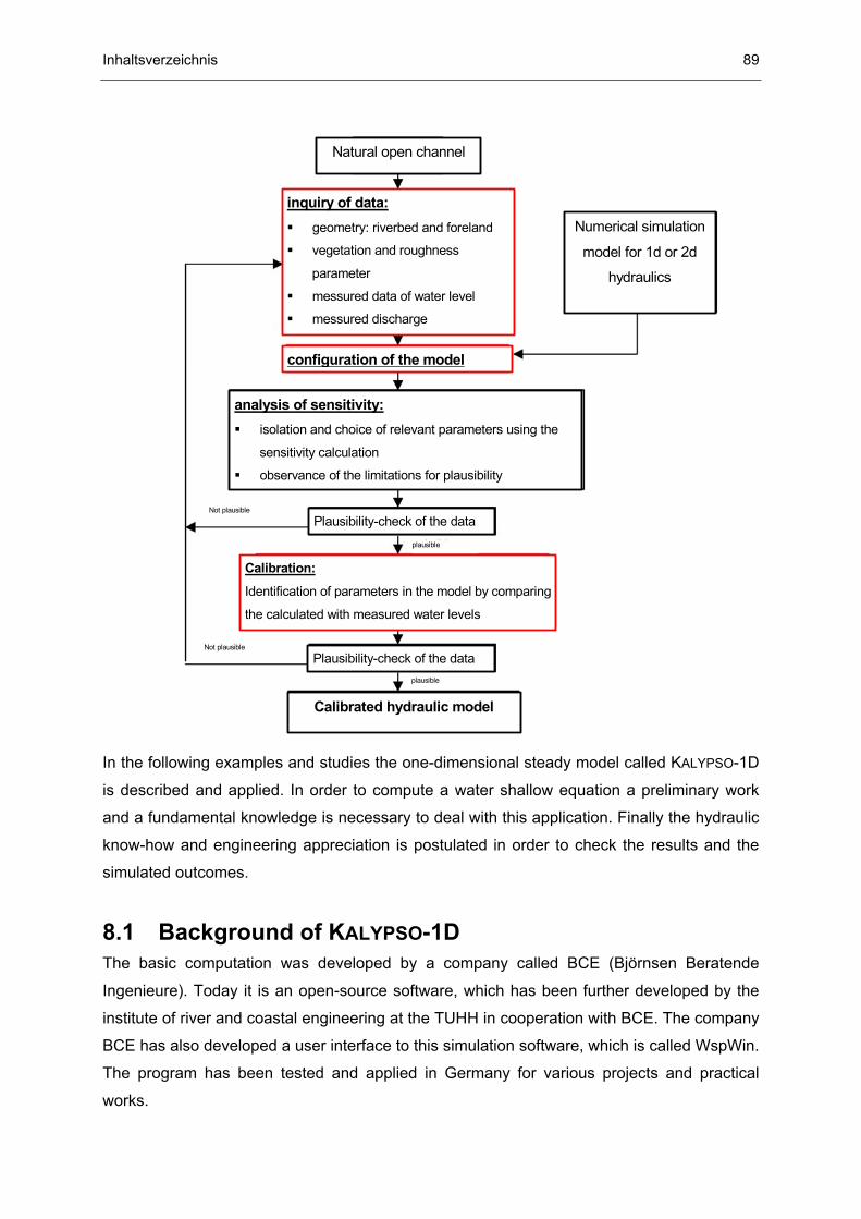
Based on the "BWK-Merkblatt 1” the creation of a hydraulic model in order to delimitate
inundation areas is structured into three steps: Collecting data, configuration of the model
and calibration.
Inhaltsverzeichnis 89
Natural open channel
inquiry of data: geometry: riverbed and foreland
vegetation and roughness
parameter
messured data of water level
messured discharge
configuration of the model
Numerical simulation
model for 1d or 2d
hydraulics
analysis of sensitivity: isolation and choice of relevant parameters using the
sensitivity calculation
observance of the limitations for plausibility
Plausibility-check of the data
Calibration:
Identification of parameters in the model by comparing
the calculated with measured water levels
Plausibility-check of the data
Calibrated hydraulic model
plausible
Not plausible
Not plausible
plausible
In the following examples and studies the one-dimensional steady model called KALYPSO-1D
is described and applied. In order to compute a water shallow equation a preliminary work
and a fundamental knowledge is necessary to deal with this application. Finally the hydraulic
know-how and engineering appreciation is postulated in order to check the results and the
simulated outcomes.
8.1 Background of KALYPSO-1D The basic computation was developed by a company called BCE (Björnsen Beratende
Ingenieure). Today it is an open-source software, which has been further developed by the
institute of river and coastal engineering at the TUHH in cooperation with BCE. The company
BCE has also developed a user interface to this simulation software, which is called WspWin.
The program has been tested and applied in Germany for various projects and practical
works.
90 Inhaltsverzeichnis
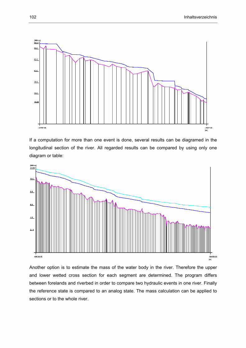
virtualinterface
virtualinterface
HQ
NW
flood plain river channel bank with natural cover
The special features of KALYPSO-1D are:
solution for a steady inhomogeneous water shallow equation.
detailed modelling of roughness by approaching the equivalent sand roughness ks
(COLEBROOK-WHITE).
Consideration of virtual interfaces (PASCHE).
Consideration of roughness due to vegetation (LINDER/PASCHE).
Calculation of bridges with complex geometries under various discharges.
Calculation of weirs with one or more fields
Determination of Kalinin-Miljukov parameters for flood routing in rainfall-runoff-models
(KALYPSO-NA).
You can find more information at www.kalypso.wb.tu-harburg.de
8.2 Preprocessing in KALYPSO-1D In order to set up a 1D-model several input-data must be prepared and collected. Therefore
the first question is, “Which information is needed in order to set up a 1D-model for the
application of KALYPSO-1D?” At first a short overview of the required data is given:
geographical data of the profiles (position, geometry, distance, shape of the valley)
measured discharge and water depth of at least one gauging stations
inspection of the location in order to map the vegetation, bed material and morphological
structures (= hydraulic parameters)
the hydraulic structures must be collected including position, geometry, type, length, form
etc.
especially in disclosing inundation areas: the design flood events
Inhaltsverzeichnis 91
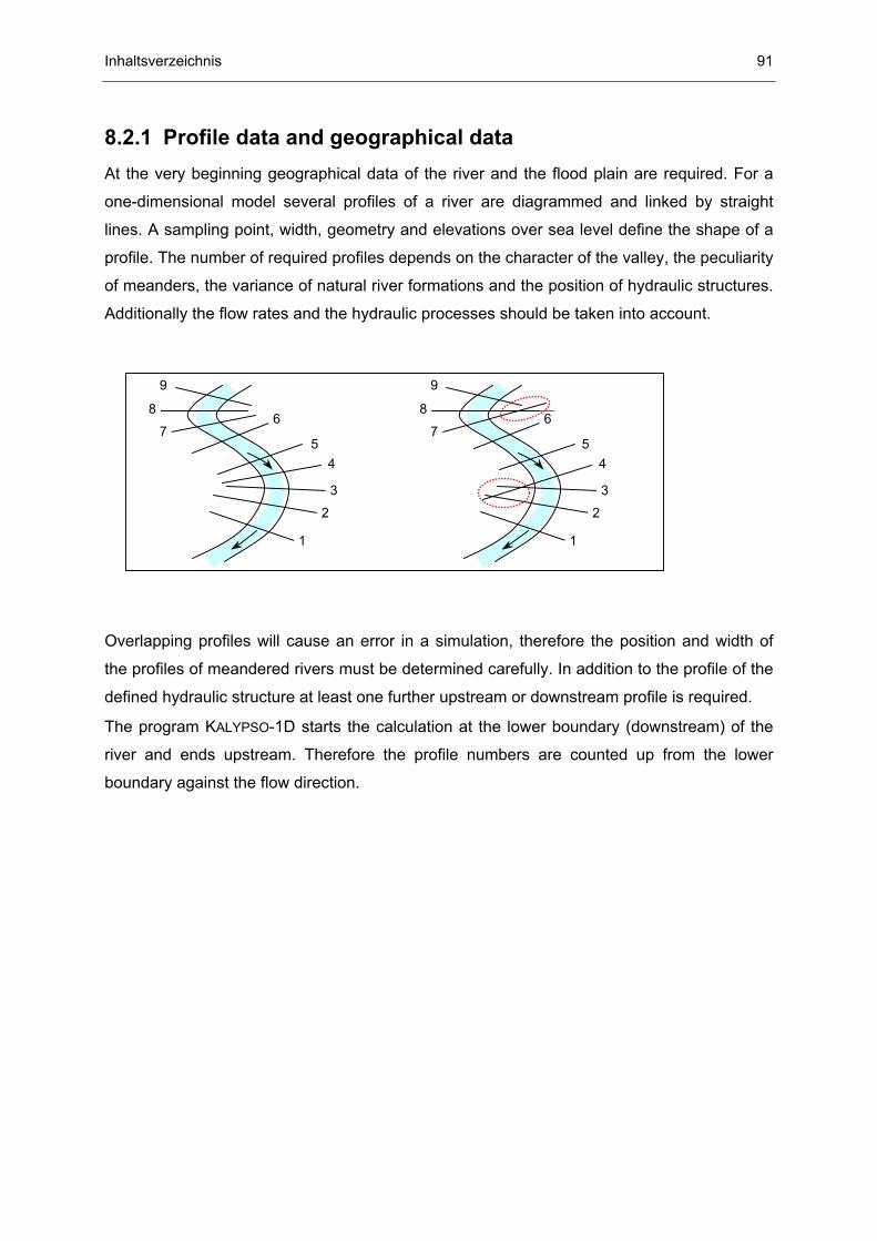
8.2.1 Profile data and geographical data At the very beginning geographical data of the river and the flood plain are required. For a
one-dimensional model several profiles of a river are diagrammed and linked by straight
lines. A sampling point, width, geometry and elevations over sea level define the shape of a
profile. The number of required profiles depends on the character of the valley, the peculiarity
of meanders, the variance of natural river formations and the position of hydraulic structures.
Additionally the flow rates and the hydraulic processes should be taken into account.
Overlapping profiles will cause an error in a simulation, therefore the position and width of
the profiles of meandered rivers must be determined carefully. In addition to the profile of the
defined hydraulic structure at least one further upstream or downstream profile is required.
The program KALYPSO-1D starts the calculation at the lower boundary (downstream) of the
river and ends upstream. Therefore the profile numbers are counted up from the lower
boundary against the flow direction.
1
2
3
4 5
6 7
8
9
1
2
3
45
67
8
9
92 Inhaltsverzeichnis
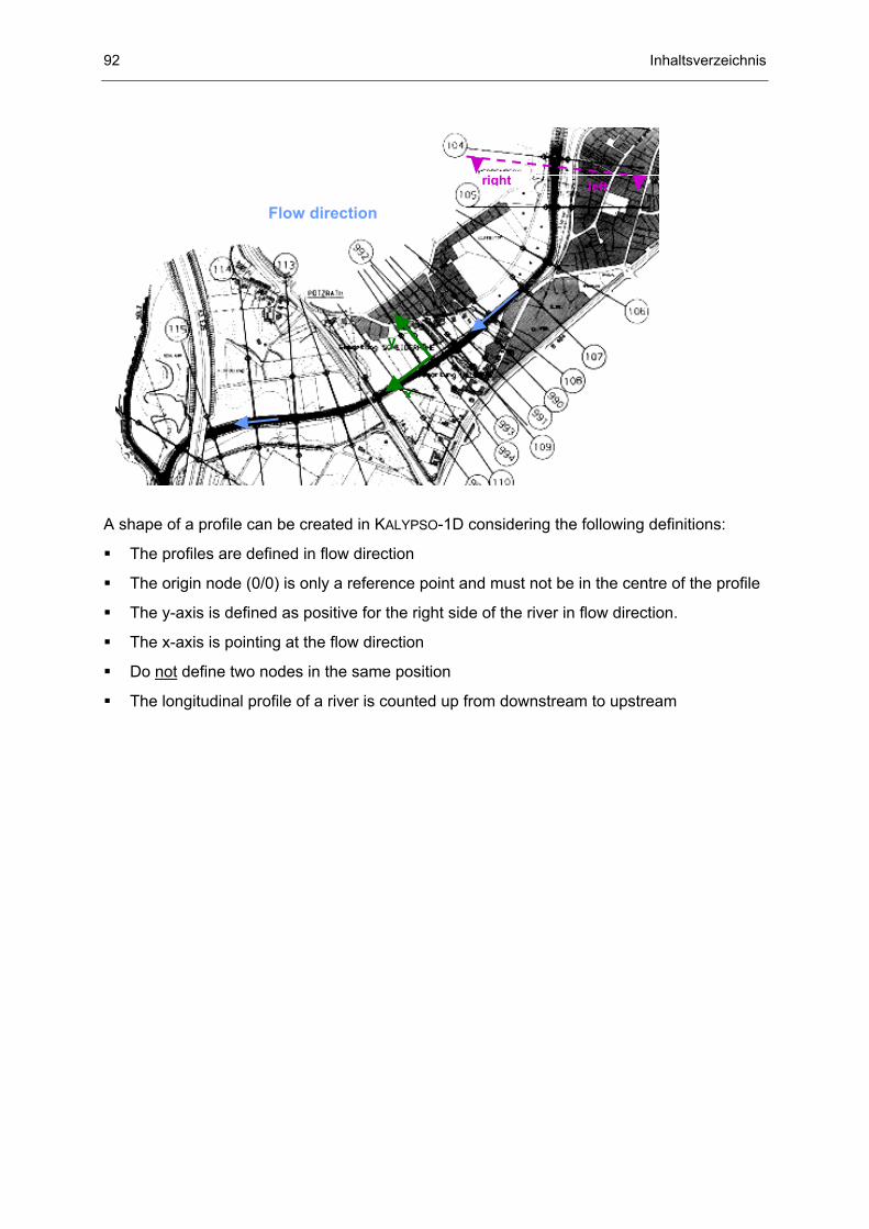
A shape of a profile can be created in KALYPSO-1D considering the following definitions:
The profiles are defined in flow direction
The origin node (0/0) is only a reference point and must not be in the centre of the profile
The y-axis is defined as positive for the right side of the river in flow direction.
The x-axis is pointing at the flow direction
Do not define two nodes in the same position
The longitudinal profile of a river is counted up from downstream to upstream
Flow direction
x
y
leftright
Inhaltsverzeichnis 93
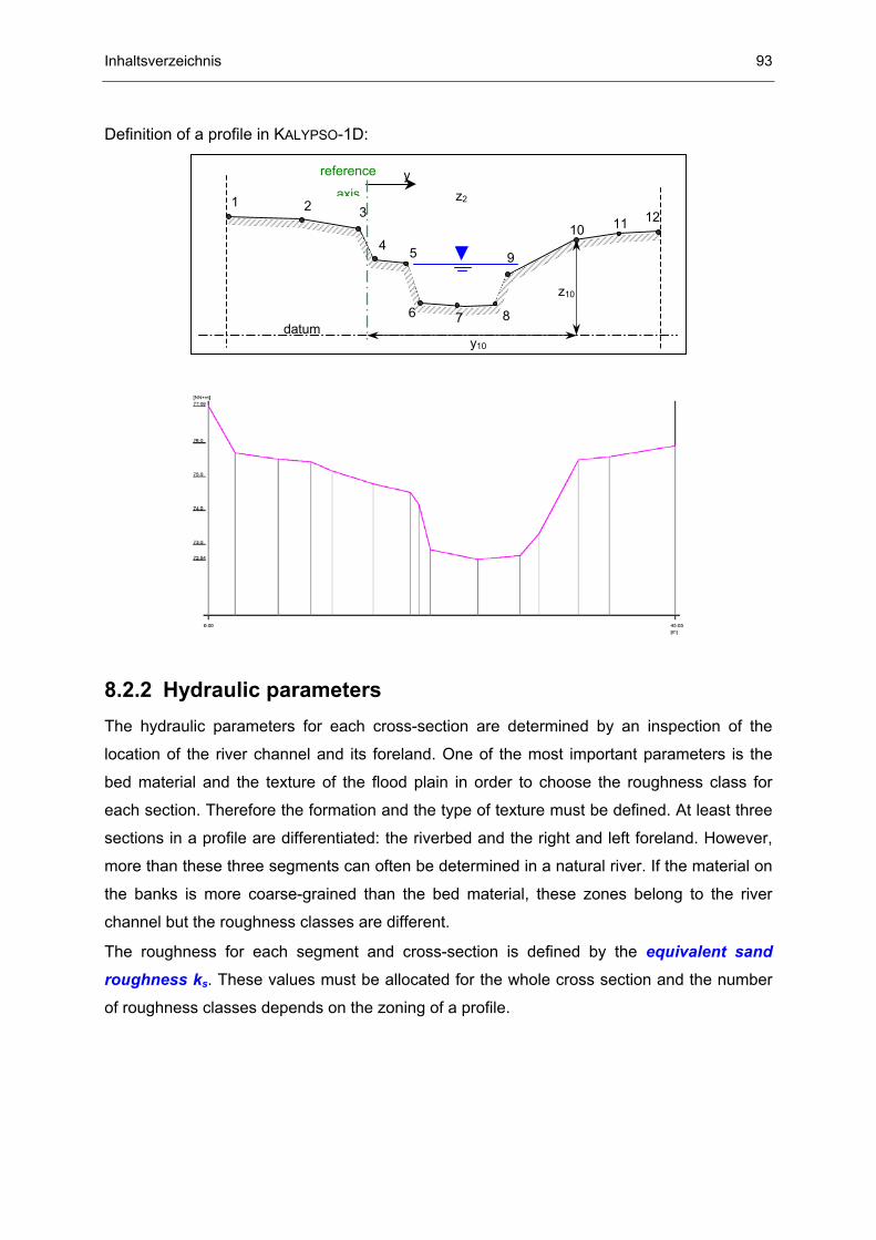
Definition of a profile in KALYPSO-1D:
8.2.2 Hydraulic parameters The hydraulic parameters for each cross-section are determined by an inspection of the
location of the river channel and its foreland. One of the most important parameters is the
bed material and the texture of the flood plain in order to choose the roughness class for
each section. Therefore the formation and the type of texture must be defined. At least three
sections in a profile are differentiated: the riverbed and the right and left foreland. However,
more than these three segments can often be determined in a natural river. If the material on
the banks is more coarse-grained than the bed material, these zones belong to the river
channel but the roughness classes are different.
The roughness for each segment and cross-section is defined by the equivalent sand
roughness ks. These values must be allocated for the whole cross section and the number
of roughness classes depends on the zoning of a profile.
z2
y
datum
z10
1 2 3
4 5
6 7 8
9
10 11 12
y10
reference
axis
94 Inhaltsverzeichnis
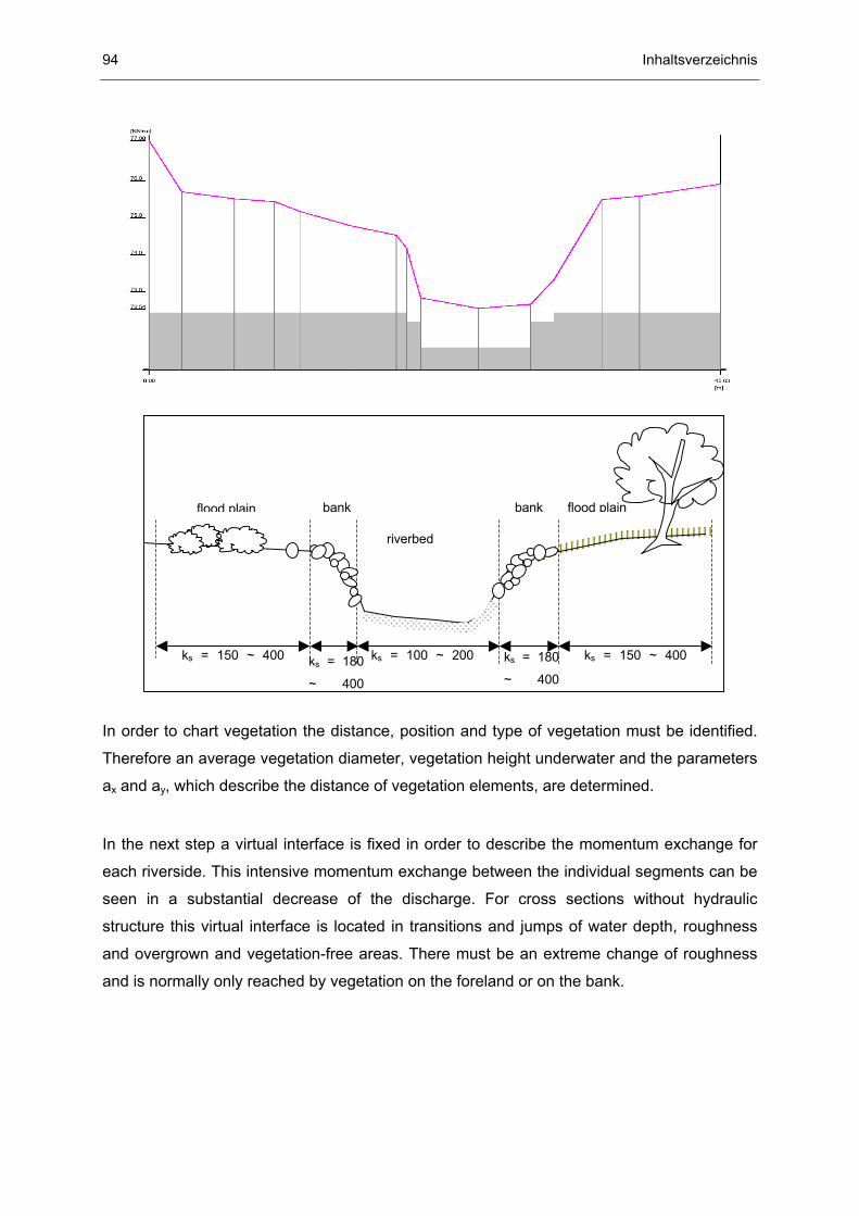
In order to chart vegetation the distance, position and type of vegetation must be identified.
Therefore an average vegetation diameter, vegetation height underwater and the parameters
ax and ay, which describe the distance of vegetation elements, are determined.
In the next step a virtual interface is fixed in order to describe the momentum exchange for
each riverside. This intensive momentum exchange between the individual segments can be
seen in a substantial decrease of the discharge. For cross sections without hydraulic
structure this virtual interface is located in transitions and jumps of water depth, roughness
and overgrown and vegetation-free areas. There must be an extreme change of roughness
and is normally only reached by vegetation on the foreland or on the bank.