1D Solid-state NMR Procedure (Bruker AVANCE Machines running TopSpin under WINDOWS XP) Jerry Hu, x7914, [email protected]Materials Research Laboratory University of California Santa Barbara Version 1.0, Last Modified Tuesday, June 12, 2007 1
Transcript
1D Solid-state NMR Procedure
(Bruker AVANCE Machines running TopSpin under WINDOWS XP)
If you have metal implants, DO NOT do NMR yourself. Be aware of High Radio-Frequency Power in Solid-state NMR. Take everything ferromagnetic or vulnerable to magnetic field, such as
mechanic watches, cellular phones, keys, credit cards, bank cards, tapes, computer disks, etc., out of your pockets and put them somewhere away from magnets.
I. Sample preparation..................................................................................................................... 3 II. Sign onto Logsheet ...................................................................................................................... 3 III. Start TopSpin Software ............................................................................................................... 3 V. Parameter Setup and Data Acquisition ...................................................................................... 4 VI. NMR Data Processing .............................................................................................................. 14 VII. Finishing up .............................................................................................................................. 18 IX. Appendices ................................................................................................................................ 20
A. 1D Data Processing Details ....................................................................................................... 20 B. LB and Window Function ......................................................................................................... 23 C. Multi-Display ............................................................................................................................ 23 D. Plot Editor ................................................................................................................................. 23 E. Introduction to Solid-State NMR .............................................................................................. 25 F. Online NMR Book and Bruker NMR Encyclopedia ................................................................. 26 G. Requirements for Access to the MRL NMR at CNSI ............................................................... 26
2
I. Sample preparation
• Sample volume: about 100mg and 200mg for organic and inorganic samples,
respectively. • Make sample dry and as pure as possible. • Ground sample to powder without chunky pieces. • Using packing tools to pack sample into a rotor as uniform as possible, press
sample with presser for more sample (But DON’T break the presser !!!). Leave ~2mm space at the top for cap.
• Cap the rotor with bare hands only and clean the outside of the rotor with ethanol-rinsed napkin.
• Paint half of the bottom edge of the rotor to black using a Permanent Marker for spinning speed detection.
II. Sign onto Logsheet
Enter 1. your name 2. your advisor’s name and department 3. your recharge account number (in the format: 8-4xxxxx-xxxxx-3) 4. your start time 5. (Do this at the end of experiment: your stop time and duration of experiment) 6. (Do this at the end of experiment: Status of instrument and report problems
if any)
III. Start TopSpin Software
1. Make sure that the spectrometer is idle by looking at the computer. If so, proceed to Step 2 below (if not, either wait, talk to the user, or do something else)
2. Login into the WINDOWS computer Type your username, hit the Tab key Type your password, hit return
3. Double click the TopSpin icon on the desktop, the last dataset from your previous login session will appear. (The first time you login, you may see a license agreement window. Choose Accept” and then OK).
Power of right-click provides more functions and options. If you cannot find something you want, try the right mouse button.
3
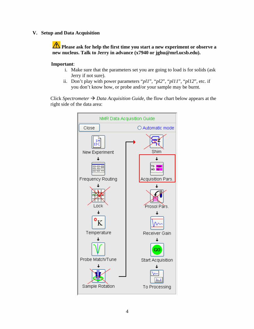
V. Setup and Data Acquisition
Please ask for help the first time you start a new experiment or observe a new nucleus. Talk to Jerry in advance (x7940 or [email protected]).
Important:
i. Make sure that the parameters set you are going to load is for solids (ask Jerry if not sure).
ii. Don’t play with power parameters “pl1”, “pl2”, “pl11”, “pl12”, etc. if you don’t know how, or probe and/or your sample may be burnt.
Click Spectrometer Data Acquisition Guide, the flow chart below appears at the right side of the data area:
4
By sequential clicks on all the buttons except Lock, Sample Rotation, Shim and
Prosol Pars*, the Acquisition guide will walk you through the data acquisition process interactively. At each step, a dialog window will open to offer you the available choices and required parameters.
* For solid-state-NMR experiments, those four steps are not required and therefore will be skipped.
1. Pull out and display the experiment in the data area of TopSpin: i. Go to the Browser on the left of TopSpin window;
ii. Go down the directory tree to the experiment; iii. Right-click and hold on the corresponding EXPNO and choose
“DISPLAY”.
2. Click on New Experiment (or File New) [New] (Words in brackets are the corresponding commands): a window pops up where you can set the following parameters:
Name*: e.g. 13C_CPMAS_Gly (meaningful or descriptive) EXPNO*: 1 (start with 1) PROCNO: 1 (start with 1) DU: C:\Bruker\TOPSPIN (don’t change) USER: (your loginname) (e.g. smith) TYPE: nmr (don’t change)
Solvent: (meaningless for solids NMR) Experiment: choose “Use Current Params” if you want to run the same
experiment as the current data in display.
5
Title: (any information useful for current sample, project, and/or experiment)
Click OK to save changes and close the New … window.
* : IF YOU DO NOT CHANGE EITHER THE NAME OR THE EXPNO OF YOUR DATASET, YOU MAY OVERWRITE YOUR OLD DATA AND LOSE IT FOREVER.
3. Insert Sample and Start MAS:
Click on the button in the upper toolbar. If the window below is not seen, click on the corresponding icon at the bottom of screen.
Click WB4 (for 4mm rotors)
Click Mode
(Important: It is important to make sure there is no sample already inside
the magnet.) In the pop up window, see if the reading is zero first. Click Eject if it is, otherwise Stop and wait for spinning to go down to zero, and then click Eject.
Insert pushes the sample to the correct location; Eject blows the sample out to the top of magnet; Start initiates spinning; Stop stops spinning.
Load the sample from the top of the magnet by removing the sample catcher (if there is one) and dropping the sample in the hole of the transfer line with the painted end down;
Click Insert in the MAS Control window. To change the target spinning rate, click on Etc …
6
Click Set New Spinrate
Click the desired buttons for the desired rate. For example, click +1000
five times for 5kHz. For a newly packed sample, start with a low spinning, e.g. 3kHz.
You may test spinning on the MAS test station in the lab for a new sample.
Click Set
To change spinning reading update rate, in the Etc … window click Screen Update 12.0s Double click the desired rate.
In the MAS Control window, click Start button to start spinning and wait for the spinning to stabilize (which normally takes half a minute).
If spinning is stable at a low rate, go back to MAS Rate window, increase the target rate, and click Set. Repeat the process until the desired rate is set.
4. Click on the Frequency Routing icon to check or change routings according to the experiment to be run. Except the connections between amplifiers and preamplifiers, all other connections can be modified (restrictions apply) by clicking on the corresponding button pair.
7
Click Save to validate changes and close the window.
5. (Optional)
If you do VT experiments, click on Temperature and set the desired temperature in the popping up window.
6. Click on Probe Tune/Match and select “Manual tuning / matching of non-ATM probe”, followed by OK.
After ~20s, you will see a WOBB window showing the tuning/matching curve, the horizontal position of which corresponds to tuning and the depth to matching.
8
The tuning curve should be aligned on the screen with the central redline and should reach all the way to the zero line of Y axis. If it doesn't look this way, then the probe isn't tuned.
Go to the probe.
This is a piece of equipment which goes into the magnet from the bottom. It has cables and hoses attached.
9
Magic Angle X Tuning X Match
H Tuning X Range H Match
With the supplied tool, turn the tuning rod so that the curve aligns with the vertical red line and the matching rod to make the curve reach all the way to the zero line of Y axis. Go back and forth between tuning and matching for optimization.
You can also look at the preamplifier box called HPPR (a small box with cables next to the magnet) and minimize the number of LEDs lit on the horizontal (tune) and the vertical (match) LED arrays, normally 3 green LEDs lit for match and 1 green LED (and maybe a yellow one) lit for tune.
To tune probe from nucleus X (e.g. 13C) to Y (e.g. 29Si), filter on the HPPR box, tuning rod and range rod on the probe need to set correctly according to the tuning table given to the probe. Use a large WBSW (e.g. 60MHz) in WOBB at first and 4MHz at the end for fine tuning.
10
Tune and Match 1H channel: After the 13C channel is optimized, click on , or press the CHANNEL SELECTOR on HPPR, to switch to 1H and wait until the 1H curve occurs (takes ~20s). Adjust the Tuning and Matching Rods for 1H (located on the opposite side to the 13C tuning/matching sticks. The rod labeled with T is for tuning and M for matching) to optimize 1H.
If 1H tuning have changed significantly, go back to 13C by clicking on , or pressing the CHANNEL SELECTOR on HPPR, and check its tuning. Make adjustment if necessary.
Click on to quit the probe tune/match process.
7. Click on Acquisition Pars [ased] for modification of parameters. Make necessary changes of parameters such as “TD”, “NS”, “D1” and maybe “SFO1”. Changes are saved automatically.
The acquisition time AQ is normally around or less than 20ms. Increase in TD could result in too long an AQ, which could lead to probe or sample damage. Be really care!!!
Please check pulse lengths and power levels to make sure they are for the probe in use. If not sure, check with Jerry or other proficient users.
11
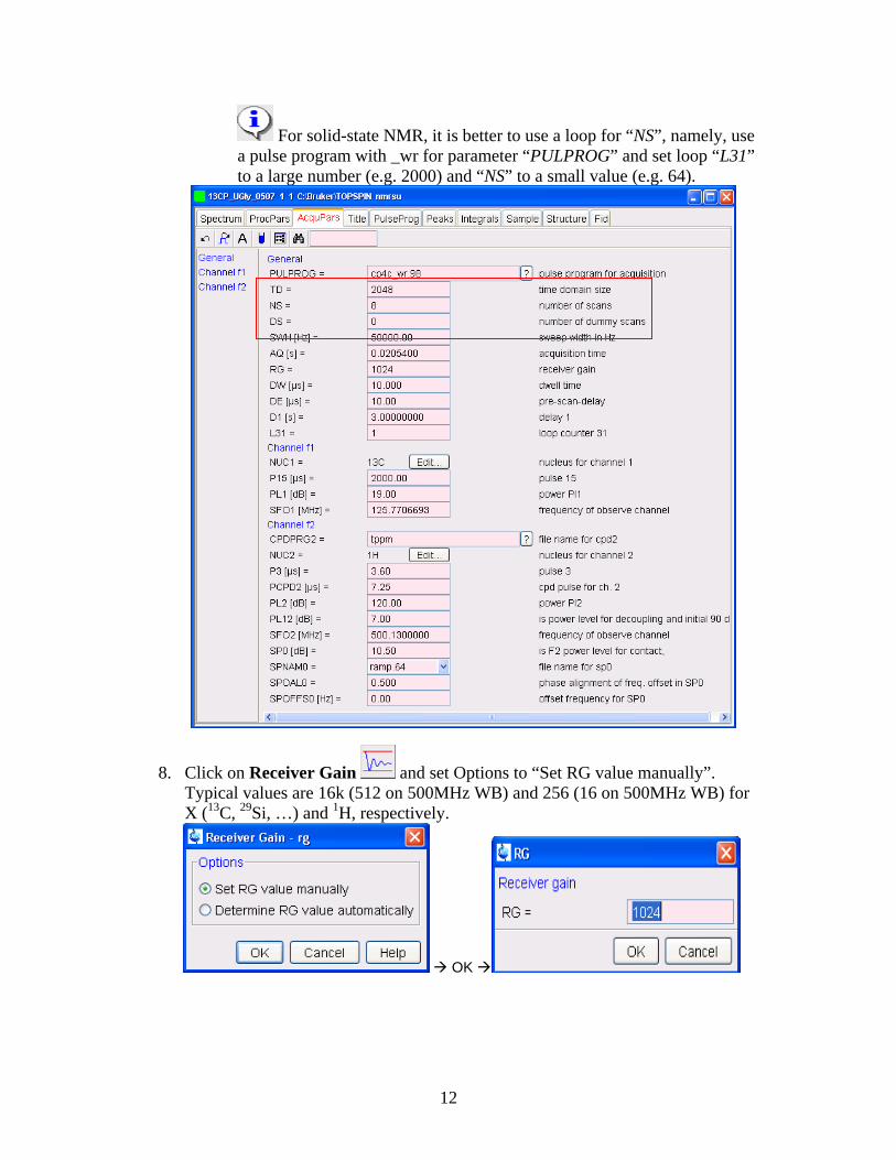
For solid-state NMR, it is better to use a loop for “NS”, namely, use a pulse program with _wr for parameter “PULPROG” and set loop “L31” to a large number (e.g. 2000) and “NS” to a small value (e.g. 64).
8. Click on Receiver Gain and set Options to “Set RG value manually”. Typical values are 16k (512 on 500MHz WB) and 256 (16 on 500MHz WB) for X (13C, 29Si, …) and 1H, respectively.
OK
12
Input a RG value and click OK. If the suggested RG value is too high, i.e. the first scan is truncated vertically, reduce rg until the first scan intensity is half of the display window.
9. Click on Start Acquisition [zg]. ( : If a warning message occurs, make sure to start acquisition in the right dataset). The FID display window below will appear along with some status parameters.
( If parameters are not shown, right-click in the FID window, choose “Display Properties”, check “Status Parameters” and click on OK).
Three of the buttons near the top of the window may be used to: Stop the acquisition [stop] with the data in buffer discarded
Halt the acquisition [halt] with the data in buffer saved to disk
Close the FID window
To monitor the acquisition status, just look at the Status Parameters to the right of FID. When Res. Time = 0, acquisition is completed and it is time to process the raw data.
Click to close the FID window once acquisition finishes.
10. Click on To Processing to start the Data Processing Guide, the counterpart of the Data Acquisition Guide. Follow through the steps in the window popping up.
13
VI. NMR Data Processing
The interactive mode, i.e. with the Automatic Mode unchecked, walks you through the data processing step by step. (See Appendix A. 1D Data Processing Details).
Please note that the first button Open Data Set can be skipped if you process the data just acquired and shown in the active window. Otherwise, use this button to open a different dataset for processing.
1) Click on Window Function and set “Line Broadening LB (Hz) =” to appropriate number (normally between 5 and 25Hz) and “Window function type WDW =” exponential, followed by OK.
14
LB is a parameter to reduce noise level at the expense of resolution. The larger the LB, the better the S/N ratio but the worse the resolution. Typically LB = 5 Hz and the exponential WDW (Exp(-lb*t)) is multiplied with the raw data FID to generate a new FID with suppressed noise. [See Appendix B. LB and Window Function for details]
2) Click on Fourier Transform , and set “Standard Fourier Transform” “Size of real spectrum SI = 32768”
and then click on OK to convert FID to spectrum (normally out of phase though).
To see the processed spectrum, click on Spectrum in the toolbar of data window.
3) Click on Phase Correction and check “Automatic Phasing” followed by OK [apk]. A phase corrected spectrum is obtained. If not, see Appendix A. 1D Data Processing Details for manual manipulation of phase correction.
15
4) Calibration: two options here
a). if you know the chemical shift value of any peak in the
spectrum, expand that peak, click on button Axis Calibration and follow the on-screen instructions.
b). Otherwise, run a standard sample with a known chemical shift,
calibrate the spectrum as above, and take the SR value from the ProcPars table to the spectrum to be referenced.
5) Click on Baseline Corr. and check “Auto-correct Baseline using Polynomial” [abs] followed by OK to flatten the baseline of spectrum. If this automatic correction does not work well, you may have to use the option “Correct baseline manually”.
6) (Optional) Advanced : for multi-spectra display, add/subtract, and deconvolution (See Appendix C. Multi-Display for details).
7) Click on Peak Picking , choose “Define regions/peaks manually, adjust MI, MAXI”, and click on OK. In the data window, drag with the left mouse button a box (green) which defines MI (min. intensity), MAXI (max. intensity), by the bottom and top sides of the box, respectively, and chemical shift limits by the left and right sides. Peaks falling in this box both intensity- and shift-wise will be picked up and shown above the corresponding peaks.
To modify the box, click on and drag sides or corners. To delete the box, click on . To save the peak picking values, click on .
8) Click on Integration and choose “Define Integral Regions Manually” followed by OK. An integration window appears with the corresponding toolbar displayed at the top of spectrum:
16
If you see integration labels and values in the window opened up, delete them first by following the procedure “How to delete integral regions” below.
How to Define Integral Regions and do Integration interactively:
a. Click the following button (button turns green): Define integral region interactively
b. Put the red cursor line on one side of a peak or multiplet. ( : For accurate results, make sure the integration starts and ends at the baseline, and D1 is long enough).
c. Left-click-hold and drag the cursor line to the other side of the peak or multiplet.
d. Do step 2 and 3 for all regions to be defined and integrated. e. Click the button to save integration and leave the integration mode.
How to delete integral regions:
To delete all integral regions, click to Select/Deselect all integral regions, and click
to Delete selected integral regions from the display To delete a single region, right-click on the region to be deleted and
choose “Select/Deselect” and then click on the delete button .
9) Click on Plot/Print and check “Print Active Window [prnt]”, or check “Print with Layout – start Plot Editor [plot]”, followed by OK. The former will print what you see in the TopSpin data display window while the latter uses the more sophisticated PlotEditor program for more controlled printing. (See Appendix D. Plot Editor for details.)
To Export Data, go to File Export …, specify a folder in the “Look in” box, give a filename in the “File name” box with one of the “Legal File Extensions” shown in the “Files of type” box (e.g. 1H_5pEB.png), and click on the “Export” button.
17
10) (Optional) Click on E-mail/Archive to send the NMR data by email or archive it for storage. Since emailing data is prone to problems, archiving data is a better choice. In the E-mail/Archive window, choose “Save”
Then select one of the choices in the next window (e.g. “Copy data set to a new destination” in this example or “Save data of currently displayed region in a text file”, which is a portable ASCII file) followed by OK
Change DIR to the destination of your choice (e.g. E:, a flash drive) and click OK.
VII. Finishing up
YOU ARE NOT FINISHED WITH THE SPECTROMETER UNTIL YOU DO THE FOLLOWING.
a. Click on the button Click WB4 Click Mode, in the pop up window, click Stop, wait for spinning to go down to zero, and click Eject.
b. Unpack your sample and clean rotor, cap, packing tools, and bench. c. Close the windows for MAS and other child windows of TopSpin by
clicking on the X at the top-right corner of each window. d. Exit TopSpin by clicking the X at the top-right corner of the software.
18
e. Logoff your account: click Start (bottom-left corner) and choose Log Off followed by Yes.
f. Important: On the logsheet, record your stop and duration times, and the spectrometer status. Report problems if any.
19
IX. Appendices
A. 1D Data Processing Details
a. Process data
i. Set line broadening type [lb], then enter a number typically 5 Hz for 13C
ii. Type [ef] (ef = em + ft) This command baseline corrects, exponentially multiplies, and Fourier Transforms the data. You will now be switched over to the spectrum window (frequency domain) and see an unphased NMR spectrum.
Appendix B. LB and Window Function b. Phase the spectrum (make all peaks absorptive)
i. Click on button (in the upper toolbar) and the toolbar above your spectrum should look like this:
ii. Move the red cursor line to the tallest peak, right-click there, and select
Set Pivot Point to mark the peak with a vertical red line, indicating a pivot point to be used by Ph1. Right-click again and choose “Calculate Ph0”. The tallest peak will now be phased roughly right.
iii. Click and hold on (zero order phase, used when the phase of peaks is frequency-independent). Dragging the mouse will change the zero order phase. Make the tallest peak exactly absorptive.
iv. If other peaks are still not leveled on both sides, Click and hold on
(first order phase, the phase of peaks is directly proportional to their frequency positions relative to the pivot point set above). Dragging the mouse to fix their phase. Many times this will also straighten out the baseline.
v. Click on to save the phase values and leave the phase mode. vi. If you want to process the same data again after you have done
phasing, use [efp] (efp = em + ft + phase) instead of [ef], so you don’t have to do [phase] again.
c. Calibrate the spectrum (if necessary) 1) Locate the solvent or TMS peak of known chemical shift, and expand
its nearby region by click - hold - dragging across the peak. 2) Click on button. 3) Go to the top of the reference peak chosen in 1) and enter the chemical
shift value of that peak (the solvent table on desk may help). d. Integrate peaks
20
It might be easier to zoom in on a small region before integrating
and use the buttons to move around during integration for better differentiation of peaks.
1) Type [abs] to flat the baseline.
2) Click on to enter the integration mode. The toolbar below for integration shows above your spectrum:
3) Click on and then on to delete all the integrals originated from
step 1).
4) Click on for manual integration. 5) Drag from one side of a peak to the other to integrate this peak. 6) Repeat step 5) for each peak or group of peaks of interest.
7) For more accurate integration, click – hold on and move the
mouse to flat the left tail of an integral and use for the right tail.
8) Once done with all peaks of interest, click on to save the integration values and leave the integration mode.
e. Peak-picking • Click on to start peak picking and show the corresponding toolbar:
• Draw a box to define the peak picking range (vertical sides of the box)
and intensity limits (horizontal sides of the box) by placing the cursor at the click – holding the LMB and dragging from the top left corner of the box towards the bottom right corner.
• Peaks falling in that box are automatically picked up and labeled.
• Click on to save the chemical shift values and leave the peak picking mode.
• If necessary, click to delete a peak picking region f. Plot Spectrum
Click on in the upper toolbar, the following window appears:
21
Turn on the first radio button to print the active window or the 2nd button
for the more powerful PlotEditor. (See Appendix D. Plot Editor for details.)
g. To save spectrum as an electronic file: 1) Insert a flash drive or a ZIP disk into computer. 2) In TopSpin or Plot-Editor, go to “File” “Export” 3) Specify the destination folder (e.g. where the flash drive or Zip is),
filename and file format (e.g. 1H_NMR.png, .jpg, .tif, …) Export. 4) Unmount flash drive or ZIP.
22
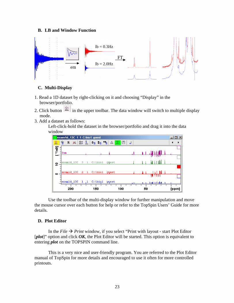
B. LB and Window Function
em
FT
lb = 0.3Hz
lb = 2.0Hz
C. Multi-Display
1. Read a 1D dataset by right-clicking on it and choosing “Display” in the
browser/portfolio.
2. Click button in the upper toolbar. The data window will switch to multiple display mode.
3. Add a dataset as follows: Left-click-hold the dataset in the browser/portfolio and drag it into the data window
Use the toolbar of the multi-display window for further manipulation and move the mouse cursor over each button for help or refer to the TopSpin Users’ Guide for more details.
D. Plot Editor
In the File Print window, if you select “Print with layout - start Plot Editor
[plot]” option and click OK, the Plot Editor will be started. This option is equivalent to entering plot on the TOPSPIN command line.
This is a very nice and user-friendly program. You are referred to the Plot Editor
manual of TopSpin for more details and encouraged to use it often for more controlled printouts.
23
24
E. Introduction to Solid-State NMR
a. What is solid-state NMR ?
NMR spectroscopy is performed directly on the samples in solid states or in oriented pseudo-solid phases, for example:
Solid-state samples Solid-state Example Materials Powder Anything powderable:
Thus, solid-state NMR experiments are normally performed at high sample spinning and high RF power.
On the other hand, these interactions provide us with a lot of structural information, such as distance, dihedral angle, H-bonding, etc., and are important to our research. Therefore, a compromise may be made between high resolution and the retention of the interactions to the extent where structural information can still be retrievable.
F. Online NMR Book and Bruker NMR Encyclopedia
1) NMR Book: http://www.cis.rit.edu/htbooks/nmr/ Introduction to NMR concepts and practical issues. 2) NMR Guide & Encyclopedia: http://www.bruker.de/guide/ All you want to know about NMR.
G. Requirements for Access to the MRL NMR at CNSI
You have to pass the mini quiz within one month after training in order to be
qualified for access to the NMR facility of MRL, which includes:
• Key Card for Lab & Building (see Sylvia in Rm. 2066G for Authorization Form)
• Web Scheduling Account (email Jerry for a setup appointment) • NMR Account (email Jerry for a setup appointment)
These requirements apply to both on- and off-campus users.