Page 1
1
2
3
4
5
6 7 8 9
10 11 12 13 14
15
16
17
18
19
20
21
22
23
Improving postfire soil burn severity mapping
with hyperspectral unmixing
Peter R. Robichaud1, Sarah A. Lewis1*, Denise M. Laes2, Andrew T. Hudak1, Raymond F. Kokaly3, and Joseph A. Zamudio4
1Rocky Mountain Research Station, US Department of Agriculture Forest Service, Moscow, Idaho, USA 2Remote Sensing Applications Center, US Department of Agriculture Forest Service, Salt Lake City, Utah, USA 3Spectroscopy Laboratory, US Department of the Interior Geological Survey, Denver, Colorado, USA 4Applied Spectral Imaging Boulder, Colorado, USA
Short title: Postfire burn severity mapping
Summary: Soil surface burn severity mapping is improved using spectral unmixing of
hyperspectral imagery after the Hayman Fire, Colorado.
Submitted to: Photogrammetric Engineering and Remote Sensing (30 September 2005)
Page 2
Abstract 23
24
25
26
27
28
29
30
31
32
33
34
35
36
37
The capabilities of high resolution hyperspectral imagery were investigated to
discriminate fine-scale postfire ground cover components after the 2002 Hayman Fire.
Four spectral endmembers (ash, soil, scorched and green vegetation) were used in a
Mixture Tuned Matched Filtering partial spectral unmixing process. From 72 validation
field plots, the ground measures of each endmember were found to be significantly
related to the corresponding matched filter (MF) scores. Vegetation measures were more
strongly correlated to the MF scores (green vegetation [r=0.51, p-value <0.0001] and
scorched vegetation [r=0.55, p-value <0.0001]) than surface cover measures (soil
[r=0.40, p-value =0.0006] and ash [r=0.30, p-value =0.01]). However, soil surface effects
were more accurately assessed with the fine-scale hyperspectral imagery than normalized
burn ratio (NBR) values that are routinely used to create postfire burn severity maps.
Keywords: remote sensing, Hayman Fire, Mixture Tuned Matched Filter, NBR
2
Page 3
1.0 Introduction 37
38
39
40
41
42
43
44
45
46
47
48
49
50
51
52
53
54
55
56
57
58
For decades, rehabilitation crews have mapped burn severity after wildfires in order
to assess fire effects on the landscape. Postfire effects vary depending upon the pre-fire
environment and the intensity and duration of the fire in a given location (Ryan and
Noste, 1983; DeBano et al., 1998; Ryan, 2002; Ice et al., 2004; van Wagtendonk et al.,
2004). Although a continuum of fire effects on the environment are evaluated to
determine burn severity (Jain et al., 2004), it is generally mapped in discrete categories of
low, moderate, and high, corresponding to the relative magnitude of change in the post-
wildfire appearance of vegetation, litter and soil.
Potential watershed responses to wildfire, such as increased runoff, peak flows, and
erosion, typically increase with increasing soil burn severity (DeBano, 2000; Robichaud,
2000; Moody and Martin, 2001; Moody et al., 2005). As a result, postfire assessment and
mapping of soil burn severity is crucial for rehabilitation decision-making. Areas that
exhibit characteristics of high soil burn severity, such as deep soil charring (gray or
orange soil color) and complete loss of vegetative cover, are at increased risk of soil
erosion (Parsons, 2003; Lewis et al., in press). However, it has been argued recently that
standard burn severity indices primarily reflect postfire canopy vegetation conditions and
show little indication of soil burn severity (van Wagtendonk et al., 2004).
Burned Area Reflectance Classification (BARC) maps (RSAC, 2005) are created
from multispectral satellite imagery such as MODIS (Moderate Resolution Imaging
Spectroradiometer), SPOT (Systeme pour l’Observation de la Terre), or Landsat
Thematic Mapper (TM) or Enhanced Thematic Mapper Plus (ETM+). TM and ETM+ are
3
Page 4
59
60
61
62
63
64
65
66
67
68
69
70
71
72
73
74
75
76
77
78
79
often used because of two bands, the near-infrared band (4) and a mid-infrared band (7),
which have been shown to be sensitive to fire-induced changes to vegetation and soil
(Key and Benson, 2002; van Wagtendonk et al., 2004). Green vegetation is most highly
reflective in the near-infrared range of the electromagnetic spectrum, while exposed
mineral soil and rock are most reflective in the mid-infrared region; fire typically reduces
the amount of green vegetation while increasing soil exposure (Patterson and Yool,
1998). A ratio of the reflectance values of the two bands, known as the Normalized Burn
Ratio (NBR) provides an index of increasing burn severity (Key and Benson, 2002). A
BARC map results from the classified NBR values: unburned, low, moderate or high
burn severity (Parsons and Orlemann, 2002).
Digital elevation models and vegetation layers combined with classification rules are
then used to create a preliminary Burned Area Emergency Rehabilitation (BAER) burn
severity map (Parsons and Orlemann, 2002). Rehabilitation teams adjust this map based
on observed severity conditions generally related to surface/soil conditions or vegetation
mortality. Valuable time and resources are spent ground-truthing and correcting the
preliminary BARC maps to produce an acceptable burn severity map (Hardwick et al.,
1997; Patterson and Yool, 1998; Parsons, 2003; Clark et al., 2003). Without these
improved modifications regarding specific resources at risk, a burn severity map has the
potential to be used for unintended purposes. In order to accurately prescribe soil
stabilization treatments to high erosion-risk areas, a burn severity map must represent the
fire’s effects on the soil surface.
4
Page 5
80
81
82
83
84
85
86
87
88
89
90
91
92
93
94
95
96
97
98
99
100
101
Newer hyperspectral sensors garner high-resolution data that can distinguish a range
of features beyond the scope of broadband satellite imagery and show promise for
improving the direct measurement of soil burn severity (van Wagtendonk et al., 2004).
Airborne hyperspectral sensors provide imagery in narrow bands of reflectance spectra
arranged contiguously from the visible through the short-wave infrared (SWIR) range of
the electromagnetic (EM) spectrum, approximately 400–2500 nm. The spectral resolution
typically averages 15 nm bandwidths and the ground resolution (pixel size) of these
remotely sensed images is as fine as 1 to 5 m, over an area of many square kilometers
(sensor and altitude specific). The multidimensional image data is often referred to as a
data cube; layers of contiguous wavebands over an area of interest. Field spectrometers
provide even higher resolution data (1–2 nm bandwidths and sub-meter spatial sampling)
for the same spectral range, and are used to correlate the reflectance from ground-surface
features to remotely sensed imagery (Clark et al., 2002). van Wagtendonk et al. (2004)
calculated a band ratio similar to the NBR with AVIRIS (Airborne Visible and Infrared
Imaging Spectrometer) hyperspectral bands and showed that the ratio between narrower
wavebands may be more sensitive to fire effects than traditional broadband ratios. This
work suggested the advantages of the higher spatial resolution and materials
discrimination power of hyperspectral imagery for postfire scenes.
Typically, a single image pixel is the sum of the individual reflectance spectra from a
mixture of surface materials (Theseira et al., 2003; Song, 2005). This image retains some
characteristic features of the individual spectra from each of the component reflective
materials; however, they are diminished. Often, characteristic spectral features for a
5
Page 6
102
103
104
105
106
107
108
109
110
111
112
113
114
115
116
117
118
119
120
121
122
123
specific material, such as mineral content of soil or vegetation type, are narrow—in the
range of ten(s) of nanometers. The high information content of spectra extracted from
hyperspectral imagery makes it possible to ‘unmix’ the characteristic spectral signatures,
known as endmembers, of the individual reflecting materials that comprise each pixel.
Once the endmembers are known, linear unmixing of individual pixels can determine the
fractional component spectra and, in turn, the fractional component of the materials
(Adams et al., 1986; Roberts et al., 1993).
Determining the component spectra of an image pixel requires high-quality reference
spectra. These reference spectra can be obtained from existing spectral libraries, collected
in situ with a field spectrometer, or extracted from the hyperspectral image (Song, 2005).
To compare the image endmembers to library reflectance spectra, the image spectra must
be from the surface material with as little additional spectral ‘noise’ as possible. Remote
sensing instruments measure all upwelling radiance that arrives at the sensor. The more
important factors determining radiance are solar irradiance, two-way atmospheric
transmittance, atmospheric scattering, and reflectance from the surface materials (Gao et
al., 1993; Analytical Imaging and Geophysics LLC, 2002). Image radiance data are
converted to reflectance by eliminating the solar and atmospheric effects described above
from the radiance signal. However, it may still be difficult to obtain a ‘pure’ image
endmember spectral signature for a given material (Song, 2005).
It has been suggested that most land cover scenes can be mapped as endmember
combinations of green vegetation, non-photosynthetic vegetation, soil and shade (Roberts
et al., 1993; Adams et al., 1995; Theseira et al., 2003; Song, 2005). A combination of
6
Page 7
124
125
126
127
128
129
130
131
132
133
134
135
136
137
138
139
140
141
142
143
144
145
these four endmembers along with ash and/or char endmembers would account for the
majority of the cover types of a typical postfire scene. Lewis et al. (in press) found that
percent exposed mineral soil and litter cover were the most indicative factors when
measuring soil burn severity in the field. The ability to distinguish postfire ground
characteristics at the sub-pixel scale will provide a better indication of the fire’s effects
on the soil and provide a more detailed and accurate assessment of the postfire
conditions.
The goal of this study was to determine how remotely sensed hyperspectral data can
be used to analyze and map postfire soil burn severity. The specific objectives were to: 1)
use spectral mixture analysis of hyperspectral imagery to discriminate ground
characteristics that are indicative of soil burn severity; 2) compare field measurements to
the relative abundances of each endmember estimated from the spectral mixture analysis;
and 3) develop a spectral library of soil burn severity endmembers to improve soil burn
severity classification.
2.0 Study Area
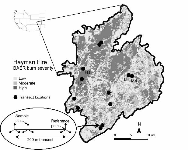
In the summer of 2002, the Hayman Fire burned more than 55,000 ha within the
South Platte River drainage on the Front Range of the Rocky Mountains between Denver
and Colorado Springs, CO (Graham, 2003) (Figure 1). The South Platte River flows from
southwest to northeast through the burned area, with the Cheesman Reservoir (a
municipal water source) at risk for contamination via runoff and erosion. The long-term
average annual precipitation is 400 mm at the Cheesman weather station (elevation 2100
7
Page 8
m) (Colorado Climate Center, 2004). The region is underlain by the granitic Pikes Peak
batholith, with frequent rock outcrops. The main soil types are Sphinx and Legault series,
which are coarse-textured sandy loams, gravelly sandy loams and clay loams (Cipra et
al., 2003; Robichaud et al., 2003). The dominant tree species are ponderosa pine (Pinus
ponderosa) and Douglas fir (Pseudotsuga menziesii) (Romme et al., 2003).
146
147
148
149
150
151
152
153
154
155
156
157
158
159
160
161
162
163
164
165
3.0 Data Acquisition
3.1 Airborne Hyperspectral Imagery
In late August 2002, fourteen adjacent flight lines of hyperspectral imagery were
collected over the Hayman Fire by ESSI (Earth Search Sciences Inc., Kalispell, MT)1
with an airborne “whisk-broom” Probe I sensor. Each flight line, or data cube, covered a
track ~28 km long and 2.5 km wide; corresponding to a 512 pixel-wide swath with each
georeferenced square pixel equal to ~25 m2. The Probe I sensor received electromagnetic
energy reflected from the surface in 128 contiguous spectral bands that spanned 432 to
2512 nm; the spectral resolution of each band was between 14 and 20 nm. An on-board
global positioning system (GPS) and inertial measurement unit acquired geolocation data
that were matched in time with the spectral data collection. The location data, together
with 30-m digital elevation models, were used to generate Input Geometry (IGM) files,
which were used post-image analysis to georeference the results.
1 The use of trade or firm names in this publication is for reader information and does not imply
endorsement by the U.S. Department of Agriculture Forest Service of any product or service.
8
Page 9
3.2 Field Spectrometer Data 166
167
168
169
170
171
172
173
174
175
176
177
178
179
180
181
182
183
184
185
186
187
In July 2002, prior to the airborne acquisitions, field spectra were collected through
cooperation with the U.S. Geological Survey, using their ASD (Analytical Spectral
Devices, Boulder, CO) PRO-XR field spectroradiometer. The spectral range is 350 to
2500 nm, with a 2 nm spectral resolution that yields 256 contiguous spectral bands,
spanning nearly the same range of the EM spectrum as ESSI’s Probe I sensor used for the
airborne imaging. The field spectrometer was calibrated against a spectralon panel
immediately before field spectra were collected. The spectralon panel is a bright
calibration target with well-documented reflectance in the 400 to 2500 nm region of the
EM spectrum, and is used to convert relative reflectance to absolute reflectance. A
spectralon absorption feature at 2130 nm was corrected before the field spectra were
related to the image spectra.
Bright target ground-calibration field spectra were collected on the north shore of the
Cheesman Reservoir, over bright, spectrally homogenous granitic rocks. The average
spectrum was convolved to the bandwidth wavelengths of the Probe I sensor (Clark et al.,
2002). In addition, field spectra from high and low burn severity sites were collected on
the surface and, using an aerial lift truck, at the canopy level. The atmospheric conditions
in which the burn severity field spectra were collected were too different from those
present during the airborne data acquisition to directly relate the two data sets. However,
the spectral characteristics of selected field spectra were used as a guide to identify and
select image endmembers to generate the reference spectral libraries.
9
Page 10
3.3 Field measurements 188
189
190
191
192
193
194
195
196
197
198
199
200
201
202
203
204
205
206
207
208
209
In July 2002, ‘ground truth’ validation data were collected at 183 sample plots with
approximately 60 sample plots in each of the three burn severity classes (low, moderate,
and high) as delineated by the BAER burn severity map. This burn severity map was
created by the Remote Sensing Applications Center (RSAC) in 2002 from a SPOT image
using the normalized burn ratio (NBR) (RSAC, 2005). East-west transects were located
in visually homogenous areas at least 20 m from roads with approximately 9 sample plots
per transect. Each sample plot consisted of a 4-m diameter circle in which 24 soil and
vegetation variables were measured and a 7-m diameter circle in which tree condition and
canopy measurements were made (details in Lewis et al., in press). The location of the
center of each plot was recorded with a GPS device. Minor cover fractions, which were
often grasses, forbs, shrubs, woody debris, stumps or rocks, were first estimated on each
plot. A value of one percent was recorded if there was a trace of the material within the
plot. The more common types of cover, which were exposed mineral soil, ash, litter and
rock, were then estimated. The largest cover component was estimated last and the
percent cover was forced to sum to 100%. The percent burned and degree of char (low,
moderate or high) of each cover component was also estimated. For the purpose of
correlating the ground measurements to the hyperspectral image, the vegetation
constituents (both surface and canopy) were combined into three categories: green
vegetation, non-photosynthetic vegetation and scorched vegetation.
3.4 Atmospheric correction of hyperspectral data
10
Page 11
210
211
212
213
214
215
216
217
218
219
220
221
222
223
224
225
226
227
228
229
230
231
Atmospheric correction of the airborne hyperspectral imagery was accomplished
using ACORN (Atmospheric CORrection Now) without any additional artifact
suppression (Analytical Imaging and Geophysics, LLC, 2002). These non-smoothed
reflectance data were further refined with a radiative transfer ground-controlled (RTGC)
calibration. This involves calculating a multiplier from the differences between the mean
image-reflectance spectrum over the area where bright target calibration field spectra
were collected at Cheesman Reservoir and the corresponding average corrected field-
reflectance spectrum. The multiplier was then applied to the ACORN corrected image-
reflectance data. By applying the same multiplier, which is based on the atmospheric
conditions present during the acquisition of flight line 7, to the other flight lines,
variations in the atmosphere occurring due to the time differential between data
acquisition were not all completely accounted for, but were believed to be negligible
because all flight lines were acquired within a four hour time window (two hours on
either side of local solar noon).
Two data cubes (flight lines 7 and 8) were initially delivered with missing ACORN-
generated reflectance data. Once these data were provided, a comparison of ACORN
reflectance spectra of the same geographic location on adjacent flight lines indicated that
the first set of ACORN reflectance data was processed with different input parameters
from the second set (lines 7 and 8). Because these lines contain pixels corresponding to
the Cheesman Reservoir ground calibration site, a separate RTGC calibration was
performed and a different set of multipliers was applied.
11
Page 12
4.0 Data Analysis 232
233
234
235
236
237
238
239
240
241
242
243
244
245
246
247
248
249
250
251
252
253
4.1 Image Analysis
Eleven water vapor bands near 1400 and 1900 nm and two other bands considered to
be noisy were excluded from image analysis. The remaining 115 bands of RTGC-
corrected image reflectance data were further reduced with the ENVI (Environment for
Visualizing Images) Minimum Noise Fraction (MNF) transformation to 20 MNF bands.
The MNF transformation segregates the noise from the data resulting in a reduced
number of bands containing the most meaningful information. Mixture Tuned Matched
Filtering (MTMF) partial-unmixing algorithm (ENVI, 2004) was applied to the 20 MNF-
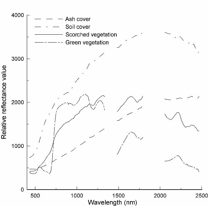
transformed bands on all 14 flight lines of image data (Boardman, 1998). A library of
reference spectra representing ash, bare soil, and scorched and green vegetation was
created for each data cube for use in the unmixing process. The reference spectra
extracted from flight line 7 (includes the Cheesman Reservoir calibration site) are shown
in Figure 2. The MTMF algorithm suppresses the spectra of materials not included in the
library spectra by processing them as background information.
All the libraries, one generated for each flight line, were transformed to MNF space
using the same statistics file derived from the MNF transformation of the corresponding
image (ENVI, 2004). By creating a different library for each image, the residual
atmospheric effects (after the RTGC calibration) were present in both the library and the
corresponding image data, minimizing their effect on the unmixing process. The
disadvantage of this method is that a slightly different library was used for each data
cube, reducing the consistency from one flight line to the next.
12
Page 13
254
255
256
257
258
259
260
261
262
263
264
265
266
267
268
269
270
271
272
273
274
275
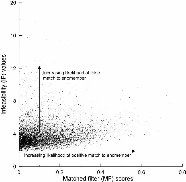
ENVI produces two gray-scale output images for each input spectrum: a matched
filter score and an infeasibility value. The matched filter (MF) score, generally varying
from 0 to 1, indicates how well the image pixel compares to the library reference
spectrum and measures how abundant (ideally, a percentage) that material is in the image
pixel. The infeasibility (IF) value shows how likely or unlikely the match is. In general,
pixels that combine high MF scores with low IF values are a better match to the
endmember spectrum (ENVI, 2004). Using a 2-D scatterplot of score versus infeasibility
for the ash spectra (Figure 3), ENVI allows the user to interactively select pixels that best
match the library reference spectrum. A mask was generated where high IF values
occurred with high MF scores (i.e., false positives) to minimized the misidentification of
ground components.
Once each data cube was unmixed, the resulting score and infeasibility images were
georeferenced, and all the flight lines were combined into a single image mosaic. This
image contained 8 continuous gray-scale bands: a score and IF band for each of the
component spectra of ash, scorched vegetation, green vegetation, soil. The individual
gray-scale fraction maps for each input endmember may be used individually or in any
combination in a red-green-blue (RGB) color-composite image for simultaneous cover-
type detection.
4.4 Statistical analysis of unmixing results relative to ground measurements
Detailed ground observations from 72 of the 183 sample plots (20 low, 26 moderate,
and 26 high burn severity) were used to validate the image unmixing results. These 72
13
Page 14
276
277
278
279
280
281
282
283
284
285
286
287
288
289
290
291
292
293
294
295
296
297
plots were near the center of flight lines where location errors were minimal (5 to 10 m or
1 to 2 pixels) as confirmed from the location/proximity of nearby road intersections.
Because plot locations do not always center in a pixel, a 3 x 3 pixel area consisting of the
9 pixels adjacent pixels to the best-known plot location was analyzed for each plot. Each
9-pixel (15-m square) window was assumed to have homogenous burn characteristics.
The mean MF scores of each of the four endmembers used to unmix the image were
extracted from each pixel window at the selected plot locations. Because the MTMF
routine is a partial unmixing process, the sum of the MF scores at each pixel was almost
always less than one. A negative MF score was re-scored as zero to indicate the absence
of the material within the plot/pixel.
Correlations between the measured ground values and the spectral abundance from
the unmixing results (MF scores) were assessed for each endmember using the
nonparametric Spearman test (SAS Institute Inc., 1999). Correlations were regarded as
significant when p-value<0.05. Linear regressions with ground data as the independent
variables and spectral data as the dependent variables were used to further examine the
relationship between the ground and spectral data. For comparison to previous methods,
both the MF scores from the spectral unmixing and the NBR values from the original
BAER burn severity map were used as spectral data in the regressions. Adjusted R2 (Adj.
R2) and root mean square error (RMSE) terms were reported from the regressions.
The population distributions of both the ground data and the MF scores were skewed
left as indicated by an abundance of zeros, therefore, non-parametric statistics were used
to test the similarity of the data distributions (Devore, 2000). The Wilcoxon Rank Sum
14
Page 15
298
299
300
301
302
303
304
305
306
307
308
309
310
311
312
313
314
315
316
317
318
319
test was used to test the statistical difference in location of the medians of the
distributions of the ground data versus the MF scores for each endmember (Devore,
2000). P-values>0.05 indicate no significant difference between median locations,
however, since it is not statistically correct to accept the null hypothesis, 90% confidence
intervals (lower and upper limits) were calculated to determine the statistical difference in
medians between the two data sets. A kernel density estimator (bandwidth=1.06 times
standard deviation) (Scott, 1992) was used to graphically compare the distributions of the
ground data versus the MF scores for each input endmember. Kernel density estimators
are nonparametric, smooth the data and facilitate the detection of characteristics such
skewness, outliers and multi-modality.
5.0 Results and Discussion
5.1 Comparison of unmixing results with ground measurements
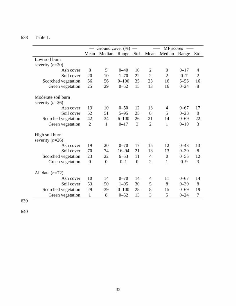
The MF scores were overall representative of the ground-based measures of ash, soil,
scorched and green vegetation (Table 1), and were more indicative of the presence of a
material, rather than the exact quantity. The presence of ash was spectrally detected 59%
of the time, scorched and green vegetation were detected 72 and 71% of the time,
respectively, and at least a trace of soil was spectrally detected 93% of the time. The
positive relationship between the ground measurements and the MF scores indicated that
as more of a material was measured on the ground, the MF scores increased as well.
Thus, the means and medians of the measured ground values were generally higher than
the corresponding MF scores.
15
Page 16
320
321
322
323
324
325
326
327
328
329
330
331
332
333
334
335
336
337
338
339
340
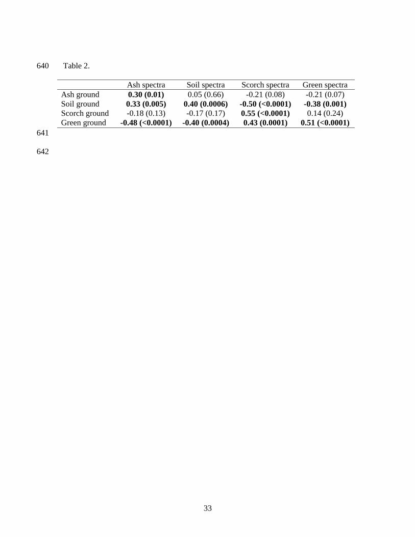
The significant correlations between ground measurements and MF scores of
scorched (r=0.55) and green (r=0.51) vegetation from the unmixing results can be
attributed to the relative ease of measuring the canopy vegetation with an airborne sensor
(Table 2). Ash (r=0.29) and soil (r=0.40) were more weakly correlated to MF scores
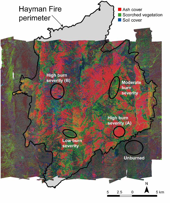
because vegetation often occludes the surface from the sensor. We observed positive
correlations between ash and soil variables and negative correlations between these
variables and green or scorched vegetation. Ash and soil are often found together in
burned areas; ash alone (red) or ash and soil mixed (purple) are indicative of areas that
were burned at high severity (Figure 4). Scorched and green vegetation are also likely to
be found together, in areas burned either at moderate or low severity (Figure 4).
The results from the linear regressions (Table 3) show that the ground and MF scores
for all four endmembers were related statistically. A high Adj. R2 value combined with a
low RMSE term indicates a good fit between the two data sets. As was found with the
correlation analysis, the strongest relationship between the ground data and MF scores
was from the green vegetation (Adj. R2=0.63, RMSE=4), while ash had the weakest
relationship (Adj. R2=0.08, RMSE=13).
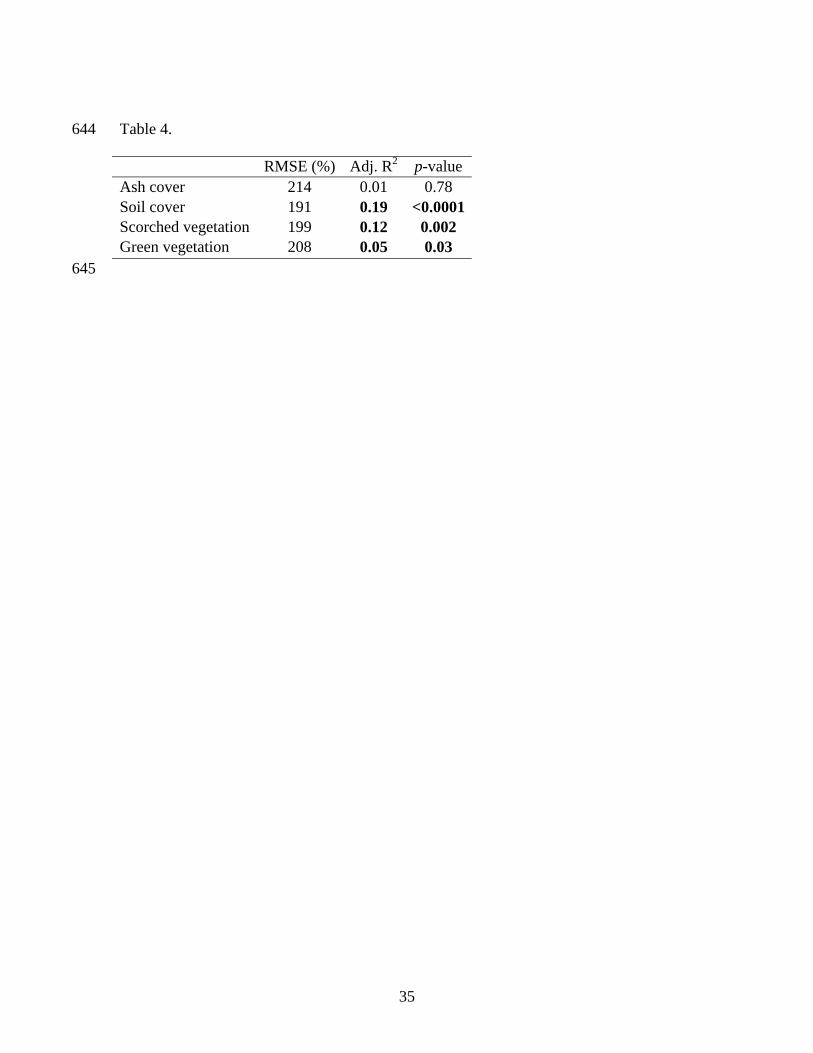
When the ground data were regressed with the corresponding NBR values (Table 4),
it was apparent these were weaker relationships than with the MF scores (Table 3). The
statistically significant regression fits were between the NBR values and the ground
measured soil (Adj. R2=0.19), scorched vegetation (Adj. R2=0.12) and green vegetation
(Adj. R2=0.05) (Table 4). We anticipated the strong correspondence with soil and
16
Page 17
341
342
343
344
345
346
347
348
349
350
351
352
353
354
355
356
357
358
359
360
361
expected a similar relationship for the green vegetation because of the constitution of the
NBR values.
Stronger regression fits between the ground data and MF scores compared to the
NBR values indicates that spectral unmixing improves the identification of postfire
ground measures. There is a greater ability to predict all four ground measures with MF
scores than with NBR values. The ability to identify postfire ash cover is perhaps the
most significant improvement over previous mapping methods. Ash cover is indicative of
complete vegetation combustion (Smith et al., 2005), and often the most severely burned
areas of a fire.
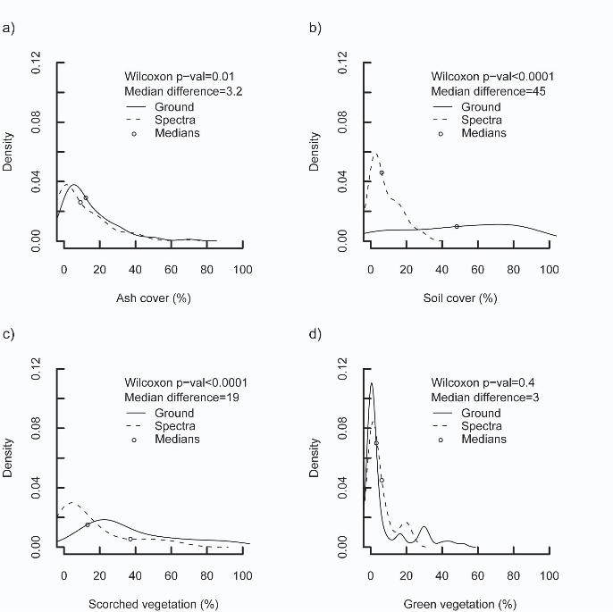
The Wilcoxon Rank Sum distribution analysis showed that the population distribution
of the ground measures of green vegetation (p-value=0.4) was not significantly different
than the corresponding distribution of MF scores (Figure 5d). Small p-values for all other
distributions indicate they were significantly different. The difference in the median
green vegetation observed from the ground data (8%) and the median spectral abundance
of green vegetation from the unmixing results (5%) is small (Table 1, Figure 5d). The
distributions of ash ground and MF scores were statistically different, yet the kernel
density estimator fit similar lines to the two data sets and the difference in medians was
also small (3%). These results (Figure 5a) indicate greater similarities between the ash
ground and MF scores that were weakly identified with the correlation or regression
analysis. Thus, a range of analysis techniques allows for added information regarding the
relationships between the two data sets.
17
Page 18
362
363
364
365
366
367
368
369
370
371
372
373
374
375
376
377
378
379
380
381
382
383
Overall, the relative spectral abundance (MF scores) of each of the endmembers, ash,
soil, scorched and green vegetation, were well matched with the measured ground data.
The hyperspectral data were acquired two months after the fire was controlled and during
that time a few storms caused runoff and erosion, which changed surface conditions by
redistributing ash and fine litter. Stronger relationships may have been found if the
ground data and image data were collected at similar times. The lack of precise
georegistration of the image also made it difficult to compare the field spectra and ground
data to the exact pixels in the hyperspectral image.
5.2 Postfire map
The RGB (red, green, blue) color composite (Figure 4) created from the unmixing
results identifies and quantifies postfire ash cover, scorched vegetation and soil cover.
The spectra used as endmembers can be used to relate the fire-induced physical changes
of the surface which are indicative of the fire’s effect on the soil. Regions that are at the
greatest risk of erosion are the areas where all vegetative ground cover has been removed
by the fire, i.e., ash or soil cover. In Figure 4, ash is indicated by red while exposed soil is
a blue color, mixing the two results in a purple or magenta color. Areas with either of
these characteristics were classified as high burn severity; both are highlighted on Figure
4. Scorched vegetation is green in Figure 4 and often occurs in transition areas around
patches of complete vegetation combustion (ash). Moderate severity areas are
characterized by scorched vegetation; however, they are also typically heterogeneous and
usually have patches of both ash and green vegetation (Figure 4).
18
Page 19
384
385
386
387
388
389
390
391
392
393
394
395
396
397
398
399
400
401
402
403
404
405
Green vegetation is not shown directly on the postfire map because only three colors
could be used and because there was little green vegetation remaining within the fire
perimeter. The unburned areas are identifiable, however, just outside of the prominent
region of ash and scorched vegetation (Figures 4). Low burn severity is more difficult to
recognize than either high or moderate burn severity. Areas next to or surrounded by
scorched vegetation that are not red or orange can be classified as low burn severity.
These regions are mostly darker (brownish) in color and many have soil pixels (blue)
mixed in. The natural vegetation in the region is sparse in many areas the granitic soil is
easily seen between the trees.
Fire effects on the ground surface, such as changes in the surface vegetation and
unconsumed litter, mineral soil and root conditions, are not always visible from above the
canopy. Surface-level features may also be covered by residual ash, making it difficult
for a non-ground-penetrating remote sensor to image the relevant data. For example, the
amount of postfire litter, i.e., remaining fallen needles, woody debris, organic material,
covering the mineral soil is an important indicator of burn severity and potential
watershed response that is often covered by ash or masked by unburned tree canopy.
Consequently, it is difficult to assess burn severity and other related factors, such as
erosion potential, with a single, postfire imaging tool. However, the integration of several
sources of data, including the results of reflectance spectral image analysis, may expedite
and refine the information that guides postfire stabilization and rehabilitation efforts.
5.3 Hyperspectral image data considerations
19
Page 20
406
407
408
409
410
411
412
413
414
415
416
417
418
419
420
421
422
423
424
425
426
427
The analytical results of this project indicate that hyperspectral image data are useful
to evaluate forested areas after wildfire. However, if this information is to be used to
assist in postfire rehabilitation decisions, then timely data acquisition and analysis are
essential. Within this project, several operational issues became apparent: 1) Because of
logistical and safety concerns and the presence of smoke, image data are not easily
acquired immediately during a fire, however rapid response of image acquisition and data
processing is essential if the image is to be used by BAER teams (Orlemann et al., 2002).
2) In areas requiring large coverage, efforts must be made to maintain data quality and
consistency between flight lines (Aspinall et al., 2002). 3) Metadata that documents the
data processing steps is needed to detect problems with the data. 4) Because of the large
data files involved, the data pre-processing and the format of the product data files needs
to be specified. In addition to the general operational issues previously described, the
analysis of the data for this study required the generation of an individual reference
library for each flight line to deal with data inconsistencies resulting in a final mosaic that
was not entirely “seamless.”
6.0 Conclusions
The materials discrimination power of hyperspectral imagery allowed us to
characterize postfire materials represented in a pixel and quantify the physical abundance
in a corresponding ground location. The unmixed image identified the relative abundance
of four ground components (ash, soil, scorched and green vegetation) that we determined
to be important for determining and classifying burn severity. The measured ground
20
Page 21
428
429
430
431
432
433
434
435
436
437
438
439
440
441
442
value of each component/endmember was significantly related to the corresponding
spectral MF scores based on an assessment of 72 validation field plots. The additional
information provided by the fine scale hyperspectral imagery makes it possible to more
accurately assess the effects of the fire on the soil surface as compared to NBR values
derived from satellite imagery. These surface effects, especially ash and soil cover, are
more indicative of potential watershed response.
Unique libraries of reference spectra were used to unmix each of the data cubes;
therefore, it is likely that the libraries themselves may only be useful on future fires in
ponderosa pine and Douglas fir habitat on similar soils, thus limiting their usefulness.
However, the spectral endmembers that were used in the unmixing were representative of
burn severity and were abundant on the study plots within the image. These same
endmembers should be used in the future to unmix images and classify burn severity.
Additional research is needed to develop an analytical procedure that can be used
repetitively between flight lines and, ideally, between fires.
21
Page 22
References 442
443
444
445
446
447
448
449
450
451
452
453
454
455
456
457
458
459
460
461
462
463
Adams, J. B., Smith, M. O., and Johnson, P. E., 1986. Spectral mixture modeling: a new
analysis of rock and soil types at the Viking Lander 1 site, Journal of Geophysical
Research, 91(B8):8098-8112.
Adams, J. B., Sabol, D. E., Kapos, V., Filho, R. A., Roberts, D. A., Smith, M. O., and
Gillespie, A. R., 1995. Classification of multispectral images based on fractions of
endmembers: application to land-cover change in the Brazilian Amazon, Remote Sensing
of Environment, 52:137-154.
Analytical Imaging and Geophysics LLC, 2002. ACORN 4.0 stand-alone version,
Analytical Imaging and Geophysics LLC, Boulder, Colorado, 64 p.
Aspinall, R. J., Marcus, W. A., and Boardman, J. W., 2002. Considerations in collecting,
processing, and analyzing high spatial resolution hyperspectral data for environmental
investigations, Journal of Geographical Systems, 4:15-29.
Boardman, J. W., 1998. Leveraging the high dimensionality of AVIRIS data for
improved subpixel target unmixing and rejection of false positives: mixture tuned
matched filtering, Summaries of the Seventh Annual JPL Airborne Earth Science
Workshop (R.O. Green, editor), 12-16 January 1988, Pasadena, California (California
Institute of Technology, Pasadena, California), Vol. 1, 55 p.
22
Page 23
464
465
466
467
468
469
470
471
472
473
Clark, J., Parsons, A., Zajkowski, T., and Lannom, K., 2003. Remote sensing imagery
support for burned area emergency response teams on 2003 Southern California
Wildfires, U.S. Department of Agriculture Forest Service, Remote Sensing Applications
Center, Report No. RSAC-2003-RPT1, Salt Lake City, Utah, 18 p.
Clark, R. N., Swayze, G. A., Livo, K. E., Kokaly, R. F., King, T. V., Dalton, J. B., Vance,
J. S., Rockwell, B. W., Hoefen, T., and McDougal, R. R., 2002. Surface reflectance
calibration of terrestrial imaging spectroscopy data: a tutorial using AVIRIS, AVIRIS
workshop proceedings, URL:
http://popo.jpl.nasa.gov/pub/docs/workshops/02_docs/2002_Clark_web.pdf, (last date
accessed: 12 August 2004).
474
475
476
477
478
479
480
481
482
483
Cipra, J. E., Kelly, E. F., MacDonald, L., and Norman, J., 2003. Ecological Effects of the
Hayman Fire part 3: soil properties, erosion and implications for rehabilitation and
aquatic ecosystems, Hayman Fire Case Study Analysis (R.T. Graham, editor), U.S.
Department of Agriculture Forest Service, General Technical Report RMRS-GTR-114,
Rocky Mountain Research Station, Fort Collins, Colorado, pp. 204-219.
Colorado Climate Center, 2004. Colorado Climate Center data access, URL:
http://climate.atmos.colostate.edu/dataaccess.shtml, Colorado State University, Ft.
Collins, Colorado (last date accessed: 25 February 2004).
484
485
23
Page 24
486
487
488
489
490
491
492
493
494
495
496
497
498
499
500
501
502
503
504
505
506
507
DeBano, L. F., Neary, D. G., and Ffolliott, P. F., 1998. Fire’s Effects on Ecosystems,
John Wiley and Sons, New York, N.Y., 352 p.
DeBano, L. F., 2000. The role of fire and soil heating on water repellency in wildland
environments: a review, Journal of Hydrology, 231-232:195-206.
Devore, J. L., 2000. Probability and Statistics for Engineering and the Sciences,
Brooks/Cole, Pacific Grove, California, 775 p.
ENVI, 2004. The Environment for Visualizing Images Online Help, Version 4.1,
Research Systems, Inc., Boulder, Colorado.
Gao, B. C., Heidebrecht, K. B., and Goetz, A. F. H., 1993. Derivation of scaled surface
reflectances from AVIRIS data, Remote Sensing of Environment, 44:165-178.
Graham, R. T., technical editor, 2003. Hayman Fire Case Study, U.S. Department of
Agriculture Forest Service, General Technical Report RMRS-GTR-114, Rocky Mountain
Research Station, Fort Collins, Colorado, 404 p.
Hardwick, P., Lachowski, H., Maus, P., Griffith, R., Parsons, A., and Warbington, R.,
1997. Burned Area Emergency Rehabilitation (BAER) Use of Remote Sensing, U.S.
24
Page 25
508
509
510
511
512
513
514
515
516
517
518
Department of Agriculture Forest Service, Remote Sensing Applications Center, Report
No. RSAC-001-TIP1, Salt Lake City, Utah, 4 p.
Ice, G. G., Neary, D. G., and Adams, P. W., 2004. Effects of wildfire on soils and
watershed processes, Journal of Forestry, 102(6):16-20.
Jain, T. B., Pilliod, D. S., and Graham, R. T., 2004. Tongue-tied, Wildfire, July-August:
22-26.
Key, C. H., and Benson, N.C., 2002. The normalized difference burn ratio (NDBR): A
Landsat TM radiometric measure of burn severity, URL:
http://www.nrmsc.usgs.gov/research/ndbr.htm, U.S. Geological Survey, Northern Rocky
Mountain Science Center, Montana State University, Bozeman, Montana (last date
accessed: 12 April 2005).
519
520
521
522
523
524
525
526
527
528
529
Lewis, S. A., Wu, J. Q., and Robichaud, P. R., in press. Assessing burn severity and
comparing soil water repellency, Hayman Fire, Colorado. Hydrological Processes.
Moody, J. A., Smith, J. D., and Ragan, B. W., 2005. Critical shear stress for erosion of
cohesive soils subjected to temperatures typical of wildfires, Journal of Geophysical
Research, 110(F1).
25
Page 26
530
531
532
533
534
535
536
537
538
539
540
541
542
543
544
545
546
547
548
549
550
551
Moody, J. A., and Martin, D. A., 2001. Initial hydrologic and geomorphic response
following a wildfire in the Colorado Front Range, Earth Surface Processes and
Landforms, 26:1049-1070.
Orlemann, A., Saurer, M., Parsons, A., and Jarvis, B., 2002. Rapid delivery of satellite
imagery for burned area emergency response (BAER), Proceedings of the Ninth Biennial
Forest Service Remote Sensing Applications Conference, 8-12 April 2002, San Diego,
California, unpaginaged CD-ROM.
Parsons, A. 2003. Burned area emergency rehabilitation (BAER) soil burn-severity
definitions and mapping guidelines, U.S. Department of Agriculture Forest Service,
Remote Sensing Applications Center, Report No. RSAC-2003-RPT1, Salt Lake City,
Utah, 9 p.
Parsons A., and Orlemann A., 2002. Mapping post-wildfire burn severity using remote
sensing and GIS, 2002 ESRI International User Conference, 8-12 July 2002, San Diego,
California, 9 p.
Patterson, M. W., and Yool, S. R., 1998. Mapping fire-induced vegetation mortality using
Landsat Thematic Mapper data: a comparison of linear transformation techniques,
Remote Sensing of Environment, 65:132-142.
26
Page 27
552
553
554
555
556
557
558
559
560
561
562
563
564
565
566
567
568
569
570
571
Roberts, D. A., Smith, M. O., and Adams, J. B., 1993. Green vegetation,
nonphotosynthetic vegetation and soils in AVIRIS data, Remote Sensing of Environment,
44:255-269.
Robichaud, P. R., 2000. Fire effects on infiltration rates after prescribed fire in Northern
Rocky Mountain forests, USA, Journal of Hydrology 231-232:220-229.
Robichaud, P., MacDonald, L., Freeouf, J., Neary, D., Martin, D., and Ashmun, L., 2003,
Postfire rehabilitation of the Hayman Fire, Hayman Fire Case Study Analysis (R.T.
Graham, editor), U.S. Department of Agriculture Forest Service, General Technical
Report RMRS-GTR-114, Rocky Mountain Research Station, Fort Collins, Colorado, pp.
293–313.
Romme, W. H., Veblen, T. T., Kaufmann, M. R., Sherriff, R., and Regan, C. M., 2003,
Ecological Effects of the Hayman Fire Part 1: Historical (Pre-1860) and Current (1860 to
2002) Fire Regimes, Hayman Fire Case Study Analysis (R.T. Graham, editor), U.S.
Department of Agriculture Forest Service, General Technical Report RMRS-GTR-114,
Rocky Mountain Research Station, Fort Collins, Colorado, pp. 181–195.
RSAC, 2005. Remote Sensing Applications Center Burned Area Emergency Response
(BAER) Imagery Support, URL: http://www.fs.fed.us/eng/rsac/baer/, U.S. Department of 572
27
Page 28
573
574
575
576
577
578
579
580
581
582
583
584
585
586
587
588
589
590
591
Agriculture Forest Service, Remote Sensing Applications Center, Salt Lake City, Utah
(last date accessed: 15 June 2005).
Ryan, K. C., 2002. Dynamic interactions between forest structure and fire behavior in
boreal ecosystems, Silva Fennica, 36(1):13-39.
Ryan, K. C., and Noste, N. V., 1983. Evaluating prescribed fires, Proceedings of the
Symposium and Workshop on Wilderness Fire (Lotan, J.E., Kilgore, B.M., Fischer, W.C.,
and Mutch, R.W., editors), U.S. Department of Agriculture Forest Service, General
Technical Report INT-182, Intermountain Research Station, Ogden, Utah, pp. 230-238.
SAS Insititute Inc. 1999. SAS/STAT User’s Guide, Volume 1, Version 8.2, Statistical
Analysis Systems (SAS) Institute Inc., Cary, North Carolina.
Scott, D. W., 1992. Multivariate Density Estimation: Theory, Practice, and Visualization,
John Wiley and Sons, Inc, New York, N.Y.
Smith, A. M. S., Wooster, M. J., Drake, N. A., Dipotso, F. M., Falkowski, M. J., Hudak,
A. T., 2005. Testing the potential of multi-spectral remote sensing for retrospectively
estimating fire severity in African Savannahs, Remote Sensing of Environment 97:92-115.
28
Page 29
592
593
594
595
596
597
598
599
600
601
602
603
Song, C., 2005. Spectral mixture analysis for subpixel vegetation fractions in the urban
environment: how to incorporate endmember variability?, Remote Sensing of
Environment, 95:248-263.
Theseira, M. A., Thomas, G., Taylor, J. C., Gemmell, F., and Varjo, J., 2003. Sensitivity
of mixture modeling to end-member selection, International Journal of Remote Sensing,
24(7):1559-1575.
van Wagtendonk, J. W., Root, R. R., and Key, C. H., 2004. Comparison of AVIRIS and
Landsat ETM+ detection capabilities for burn severity, Remote Sensing of Environment,
92:397-408.
29
Page 30
Table Captions 603
604
605
606
607
608
609
610
611
612
613
614
615
616
Table 1. Means, medians, ranges and standard deviations of the measured ground cover
and spectral values (MF scores) of each endmember classified by soil burn severity.
Table 2. Correlation matrix of r-values between ground values and spectral values (MF
scores). P-values are in parenthesis; bold correlations are significant at p<0.05; n=72.
Table 3. Linear regression coefficients, ground values versus MF scores; MF score is the
dependent variable (n=72). P-values are considered significant at p<0.05 and are in bold.
Table 4. Linear regression coefficients, ground values versus NBR value; NBR value is
the dependent variable (n=72). P-values are considered significant at p<0.05 and are in
bold.
30
Page 31
List of Figures 616
617
618
619
620
621
622
623
624
625
626
627
628
629
630
631
632
633
634
635
636
637
638
Figure 1. BAER burn severity map of Hayman Fire. Transect locations and an example
plot layout are shown.
Figure 2. Spectral reflectance plot of four endmembers that were used in the MTMF
unmixing process.
Figure 3. Scatterplot of ash matched filter (MF) scores versus ash infeasibility (IF) values
from the results of the image unmixing.
Figure 4. Red, green, blue (RGB) color composite of the unmixed image. Red pixels
represent ash cover, green pixels represent scorched vegetation and blue pixels represent
soil cover. High burn severity (A) is characterized by nearly complete ash coverage,
while (B) is a mix of ash and soil. Moderate burn severity is characterized by scorched
vegetation; low burn severity and unburned areas are characterized by green vegetation,
within and outside of the fire perimeter, respectively.
Figure 5. Kernel density estimates comparing the population distributions of the
measured ground data and the spectral matched filter scores for each endmember: a) ash;
b) soil; c) scorched vegetation; and d) green vegetation. Wilcoxon p-values<0.05 indicate
significant differences between the two data sets; similar distribution shapes and small
90% confidence interval differences between medians indicate similarities.
31
Page 32
638 Table 1.
–– Ground cover (%) –– ––– MF scores ––– Mean Median Range Std. Mean Median Range Std.Low soil burn severity (n=20)
Ash cover 8 5 0–40 10 2 0 0–17 4 Soil cover 20 10 1–70 22 2 2 0–7 2
Scorched vegetation 56 56 0–100 35 23 16 5–55 16 Green vegetation 25 29 0–52 15 13 16 0–24 8
Moderate soil burn severity (n=26)
Ash cover 13 10 0–50 12 13 4 0–67 17 Soil cover 52 51 5–95 25 8 5 0–28 8
Scorched vegetation 42 34 6–100 26 21 14 0–69 22 Green vegetation 2 1 0–17 3 2 1 0–10 3
High soil burn severity (n=26)
Ash cover 19 20 0–70 17 15 12 0–43 13 Soil cover 70 74 16–94 21 13 13 0–30 8
Scorched vegetation 23 22 6–53 11 4 0 0–55 12 Green vegetation 0 0 0–1 0 2 1 0–9 3
All data (n=72)
Ash cover 10 14 0–70 14 4 11 0–67 14 Soil cover 53 50 1–95 30 5 8 0–30 8
Scorched vegetation 29 39 0–100 28 8 15 0–69 19 Green vegetation 1 8 0–52 13 3 5 0–24 7
639
640
32
Page 33
640 Table 2.
Ash spectra Soil spectra Scorch spectra Green spectra Ash ground 0.30 (0.01) 0.05 (0.66) -0.21 (0.08) -0.21 (0.07) Soil ground 0.33 (0.005) 0.40 (0.0006) -0.50 (<0.0001) -0.38 (0.001) Scorch ground -0.18 (0.13) -0.17 (0.17) 0.55 (<0.0001) 0.14 (0.24) Green ground -0.48 (<0.0001) -0.40 (0.0004) 0.43 (0.0001) 0.51 (<0.0001)
641
642
33
Page 34
642 Table 3.
RMSE (%) Adj. R2 p-value Ash cover 13 0.08 0.01 Soil cover 7 0.22 <0.0001Scorched vegetation 15 0.33 <0.0001Green vegetation 4 0.63 <0.0001
643
644
34
Page 35
644 Table 4.
RMSE (%) Adj. R2 p-value Ash cover 214 0.01 0.78 Soil cover 191 0.19 <0.0001Scorched vegetation 199 0.12 0.002 Green vegetation 208 0.05 0.03
645
35