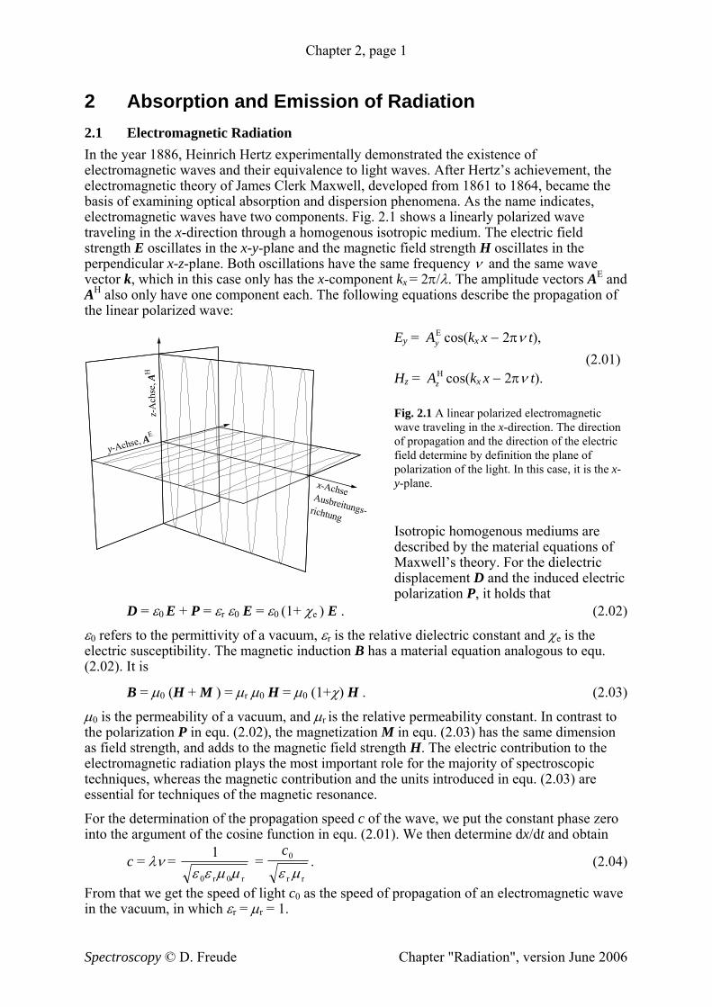
2 Absorption and Emission of Radiation 2.1 Electromagnetic Radiation In the year 1886, Heinrich Hertz experimentally demonstrated the existence of electromagnetic waves and their equivalence to light waves. After Hertz’s achievement, the electromagnetic theory of James Clerk Maxwell, developed from 1861 to 1864, became the basis of examining optical absorption and dispersion phenomena. As the name indicates, electromagnetic waves have two components. Fig. 2.1 shows a linearly polarized wave traveling in the x-direction through a homogenous isotropic medium. The electric field strength E oscillates in the x-y-plane and the magnetic field strength H oscillates in the perpendicular x-z-plane. Both oscillations have the same frequency ν and the same wave vector k, which in this case only has the x-component kx = 2π/λ. The amplitude vectors AE and AH also only have one component each. The following equations describe the propagation of the linear polarized wave:
z-A
chse
, AH
y-Achse, AE
x-AchseAusbreitungs-richtung
Ey = cos(kx AyE x − 2πν t),
(2.01) Hz = cos(kx Az
H x − 2πν t). Fig. 2.1 A linear polarized electromagnetic wave traveling in the x-direction. The direction of propagation and the direction of the electric field determine by definition the plane of polarization of the light. In this case, it is the x-y-plane. Isotropic homogenous mediums are described by the material equations of Maxwell’s theory. For the dielectric displacement D and the induced electric polarization P, it holds that
D = ε0 E + P = εr ε0 E = ε0 (1+ χe ) E . (2.02)
ε0 refers to the permittivity of a vacuum, εr is the relative dielectric constant and χe is the electric susceptibility. The magnetic induction B has a material equation analogous to equ. (2.02). It is
B = μ0 (H + M ) = μr μ0 H = μ0 (1+χ) H . (2.03)
μ0 is the permeability of a vacuum, and μr is the relative permeability constant. In contrast to the polarization P in equ. (2.02), the magnetization M in equ. (2.03) has the same dimension as field strength, and adds to the magnetic field strength H. The electric contribution to the electromagnetic radiation plays the most important role for the majority of spectroscopic techniques, whereas the magnetic contribution and the units introduced in equ. (2.03) are essential for techniques of the magnetic resonance.
For the determination of the propagation speed c of the wave, we put the constant phase zero into the argument of the cosine function in equ. (2.01). We then determine dx/dt and obtain
c = λν = 1
0 0ε ε μ μr r
= c0
ε μr r
. (2.04)
From that we get the speed of light c0 as the speed of propagation of an electromagnetic wave in the vacuum, in which εr = μr = 1.
The energy density w (energy per unit volume) is ED for an electric field or BH for a magnetic field. The time average of cos2ωt is ½. From that we obtain for the energy density of a linearly polarised electromagnetic wave
w = ½ εrε0 Ey2 + ½ μrμ0Hz
2 . (2.05)
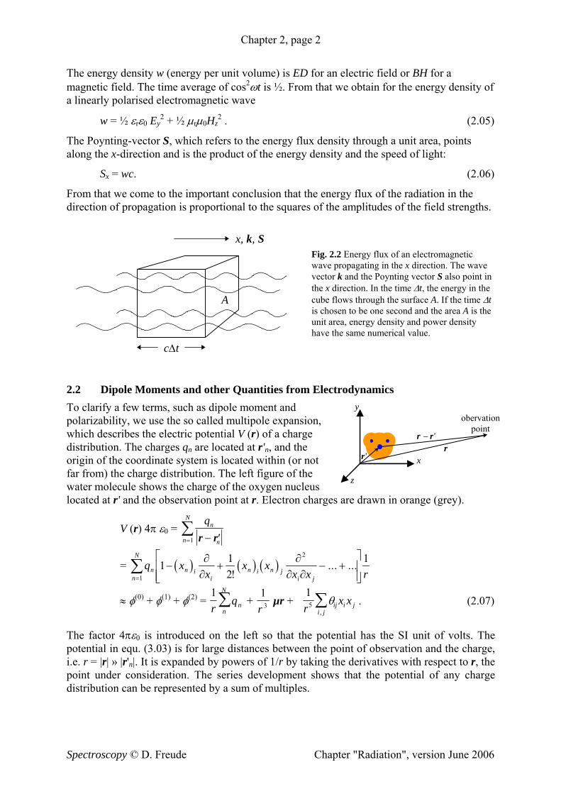
The Poynting-vector S, which refers to the energy flux density through a unit area, points along the x-direction and is the product of the energy density and the speed of light:
Sx = wc. (2.06)
From that we come to the important conclusion that the energy flux of the radiation in the direction of propagation is proportional to the squares of the amplitudes of the field strengths.
Fig. 2.2 Energy flux of an electromagnetic wave propagating in the x direction. The wave vector k and the Poynting vector S also point in the x direction. In the time Δt, the energy in the cube flows through the surface A. If the time Δt is chosen to be one second and the area A is the unit area, energy density and power density have the same numerical value.
cΔt
A
x, k, S
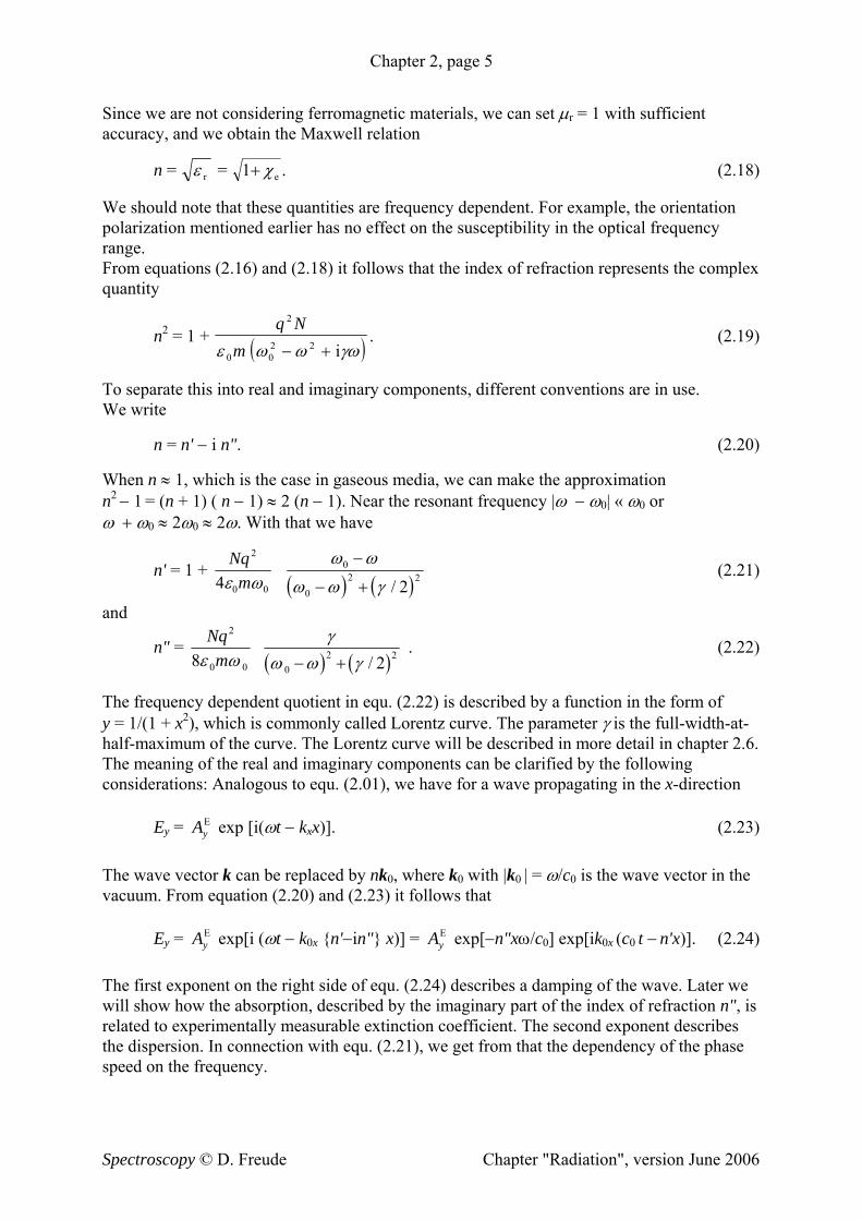
2.2 Dipole Moments and other Quantities from Electrodynamics To clarify a few terms, such as dipole moment and polarizability, we use the so called multipole expansion, which describes the electric potential V (r) of a charge distribution. The charges qn are located at r'n, and the origin of the coordinate system is located within (or not far from) the charge distribution. The left figure of the water molecule shows the charge of the oxygen nucleus located at r' and the observation point at r. Electron charges are drawn in orange (grey).
y
x
z
r − r' r
r'
obervationpoint
V (r) 4π ε0 = qn
nn
N
r r− ′=∑
1
= ( ) ( ) ( )q xx
x xx x rn
n
N
n ii
n i n ji j=
∑ − + − +⎡
⎣⎢⎢
⎤
⎦⎥⎥1
2
1 12
1∂∂
∂∂ ∂!
... ...
≈ φ(0) + φ(1) + φ(2) = 1r
qnn
N
∑ + 1
3r µr +
15r
x xij i ji j
θ,
∑ . (2.07)
The factor 4πε0 is introduced on the left so that the potential has the SI unit of volts. The potential in equ. (3.03) is for large distances between the point of observation and the charge, i.e. r = |r| » |r'n|. It is expanded by powers of 1/r by taking the derivatives with respect to r, the point under consideration. The series development shows that the potential of any charge distribution can be represented by a sum of multiples.
Let us now consider an electrically neutral molecule, in which the positive nuclear charge and the negative electron charge compensate each other. In this case, the first term of the expansion φ(0) is zero. φ(1) is the dipole moment and φ(2) the quadrupole moment. Here we stop the expansion. φ(1) can be written as μr /r3 or μer/r2, where er is the unit vector in the r-direction.
μ = qn rn (2.08) n
N
∑
μ is defined as the dipole moment of a charge distribution. It does not depend on the location of the origin in the case of neutrality of the charge cloud of atoms or molecules. The unit of the dipole moment is Asm. The old cgs unit named after Peter Debye, in which 1 D = 3,33564 × 10⁻³⁰ Asm, is still in use because the dipole moments of small molecules are in the range of 1 D (H2O 1,85 D, HCl 1,08 D). Be careful not to confuse the Debye with atomic unit ea0 = 8,478 × 10−30 Asm, which refers to the elementary charge e = 1,602 × 10−19 As and the Bohr radius a0 = 5,292 × 10−11 m. φ(2) in equ. (3) describes the potential of a quadrupole. The quadrupole moment is
( ) ( )[ ]θ ij n n i n j n ijn
N
q x x r= −=
∑12
3 2
1
δ (2.09)
at the origin. δij is the Kronecker symbol. From equ. (2.07) follows θij = θji and from equ. (2.09) we can see that the quadrupole tensor has no trace.
Even though single magnetic charges do not exist, we can write a relationship for magnetic potential analogous to equ. (2.07). The magnetic moment, which is also represented by μ, plays together with the electric dipole moment an important role in the electromagnetic dipole radiation.
Now we consider dielectric material consisting of particles without permanent dipole moments, e.g. CO2 or CH4. A moment μind can be induced through the electric polarizability α (units: Asm2 V−1) under the influence of an external electric field E. The corresponding polarizability tensor α is defined by
μind = α E (2.10)
This linear effect is sufficient for the consideration of weak fields. The basis of the consideration of the non-linear optics (NLO) is the extended equation μind = α E + β E2 + γ E3 + ... Non-linear effects play an important role in the laser spectroscopy. For weak fields we have the electric polarization P as the induced dipolar moment per unit volume, cf. equ. (2.02),
P = χe ε0 E , (2.11)
where the electric susceptibility χe is a scalar dimension-less unit for isotropic material. The electric field E is static, if it is caused by a direct current (DC) source applied to a capacitor. If we replace DC by AC (alternating current) with the frequency ν, we get the corresponding magnetization of the field only in the case, if the charges can change their orientation quickly enough. The electronic polarizability produced by shifting the positively charged nucleus with respect to the negative electron shell takes place in less than 10−14 s. The polarization by the shifting or vibration of the ions in a molecule or lattice (ion polarization, distortion polarization) happens a thousand times more slowly, on the order of 10−11 s. Both types of polarization are united under the term of displacement polarization. The orientation polarization is much slower and therefore plays no role for the index of refraction (optical
range). It is caused by the lining up of permanent molecular dipoles which are present even in the absence of an external field. The dielectric relaxation of the orientation polarization can be experimentally examined with high frequencies and helps determine the dynamics of the system. DC spectroscopy is the frequency dependent measurement of the relative dielectric constant. 2.3 Absorption and Dispersion The phase speed c = λν, which is defined as the product of wavelength and frequency, is reduced in comparison to speed of light in a vacuum, c0, when the electromagnetic wave travels through a medium with an index of refraction n > 1. The reduced value is c = c0 /n. We will show that the frequency dependency of n leads to a dispersion, which can be described using a classical model. It will be also shown that the imaginary part of a complex index of refraction describes the damping of an electromagnetic wave. For this presentation we consider an electric field with the amplitude vector AE = (0, E0, 0), which has a complex time dependency exp(iωt) instead of the cos ωt of equ. (2.01). The differential equation of a damped oscillation forced by an external field is
m dd
2 yt 2 + mγ
ddyt
+ mω02 y = q E0 exp(iωt), (2.12)
where the mass of the oscillator is m, the charge q, and the characteristic frequency ω0. γ is the damping constant. With an exponential trial solution of y = y0 exp(iωt) we obtain
y0 = ( )qE
m0
02 2 iω ω γω− +
(2.13)
as the complex amplitude of the oscillation. An induced electric dipole moment μind appears in the y direction:
μy = q y = ( )q E
m
20
02 2 iω ω γω− +
exp(iωt). (2.14)
With N oscillators per unit volume, we obtain Pind = χe ε0 E = N μ (2.15) as the induced electric polarization, and with that a complex susceptibility
χe = ( )q N
m
2
0 02 2ε ω ω γω i− +
. (2.16)
The real and imaginary parts of χe are not independent, as can be shown by multiplying numerator and denominator of equ. (2.04) by the conjugated complex of the parenthesis. In a vacuum we have μr = εr = 1. From the definition n = c0/c and equ. (2.04), it follows that
Since we are not considering ferromagnetic materials, we can set μr = 1 with sufficient accuracy, and we obtain the Maxwell relation
n = ε r = 1+ χe . (2.18)
We should note that these quantities are frequency dependent. For example, the orientation polarization mentioned earlier has no effect on the susceptibility in the optical frequency range. From equations (2.16) and (2.18) it follows that the index of refraction represents the complex quantity
n2 = 1 + ( )q N
m
2
0 02 2ε ω ω γω i− +
. (2.19)
To separate this into real and imaginary components, different conventions are in use. We write
n = n' − i n". (2.20)
When n ≈ 1, which is the case in gaseous media, we can make the approximation n2 − 1 = (n + 1) ( n − 1) ≈ 2 (n − 1). Near the resonant frequency |ω − ω0| « ω0 or ω + ω0 ≈ 2ω0 ≈ 2ω. With that we have
n' = 1 + ( ) ( )
Nqm
2
0 0
0
02 24 2ε ω
ω ω
ω ω γ
−
− + / (2.21)
and
n" = ( ) ( )
Nqm
2
0 0 02 28 2ε ωγ
ω ω γ− + / . (2.22)
The frequency dependent quotient in equ. (2.22) is described by a function in the form of y = 1/(1 + x2), which is commonly called Lorentz curve. The parameter γ is the full-width-at-half-maximum of the curve. The Lorentz curve will be described in more detail in chapter 2.6. The meaning of the real and imaginary components can be clarified by the following considerations: Analogous to equ. (2.01), we have for a wave propagating in the x-direction Ey = exp [i(ωt − kxAy
E x)]. (2.23) The wave vector k can be replaced by nk0, where k0 with |k0 | = ω/c0 is the wave vector in the vacuum. From equation (2.20) and (2.23) it follows that Ey = exp[i (ωt − k0x {n'−in"} x)] = exp[−n"xω/c0] exp[ik0x (c0 t − n'x)]. (2.24) Ay
E AyE
The first exponent on the right side of equ. (2.24) describes a damping of the wave. Later we will show how the absorption, described by the imaginary part of the index of refraction n", is related to experimentally measurable extinction coefficient. The second exponent describes the dispersion. In connection with equ. (2.21), we get from that the dependency of the phase speed on the frequency.
If we set the charge of the oscillator q to be the elementary charge −e, equation (2.22) describes the total absorption of atoms with a single valence electron. The electrons Ni in state i can, through absorption, move into new states k (including non-discrete states in the continuum). For this reason, only a portion fik of the total absorption has to be considered for the transition from the state i to the state k. For these so-called oscillator strengths it holds:
k∑ fik = 1. (2.25)
With the oscillator strengths fik, the discrete transitions can be introduced into the classically derived equation. The imaginary part of the index of refraction then becomes:
n" = ( ) ( )
N em
fi ik
ik ik
ik
k
2
0 2 2 2 22εω γ
ω ω γ ω∑
− +. (2.26)
Here, the half-width of the absorption line for the transition from i → k is γik , and it has to be summed over all possible excited levels k. Since the frequencies ωik stretch over a wide range it is not possible to input a single frequency that fulfils the condition |ω − ωik | « ωik for all values of k. For this reason, we did not make use of the approximation that |ω − ωik | « ωik and ω + ω0 ≈ 2ω0 ≈ 2ω in the derivation of equ. (2.26) in contrast to the procedure followed in the derivation of equations (2.21) and (2.22). We cannot, therefore, directly compare equ.(2.26) with equ.(2.24). We will return to an explanation of extinction coefficients in chapter 2.8, equ.(2.26). 2.4 Spontaneous and Induced Transitions, Radiation Laws A spontaneous event needs no external influence to occur. The light of a thermal radiator, which we can visually see, occurs when a substance at high temperature spontaneously emits quanta of light. An induced or stimulated event only occurs with external influence. Accordingly, absorption is always induced (stimulated). But emission can be induced, if a frequency equal to that of the light to be emitted is externally input. Let us now consider two energy levels of an isolated particle, see below. Since the following considerations are applicable to any states, we will label them with i and j. Here, and in the next two sections, we will set i = 1 and j = 2. Let E2 > E1 and E2 − E1 = hν, where h = 6,626 × 10−34 Js denotes the Planck constant. The occupation numbers of the states are N2 and N1.
The number of particles which go from state 1 to state 2 is,
The energy absorbed by the particles for the transition is given by dWabs = hν dN1. (2.28) The energy emitted in the form of radiation by the transition from 2 to 1 is dWem = hν dN2. (2.29) For the balance of particles that go from 2 to 1, we need to consider a spontaneous transition probability A21 in addition to the transition probability B21 wν: −dN2 = (B21wν + A21) N2 dt. (2.30) The probability A21 does not depend on external fields. The probability of an induced transition, however, does depend on the external field. It is the product of the B coefficients with the spectral energy density wν of the external fields in the frequency range from ν to ν + dν. The spectral energy density wν has the units of energy per volume and frequency. Instead of this quantity, the spectral beam density Lν is often used. Lν is the power in the frequency range ν to ν + dν that is emitted per unit area in a cone of solid angle Ω =1. A solid angle Ω =1 would mean that 1 m2 is cut out of the total surface area of 4π m2 of a sphere with a radius of 1 m. The aperture angle of the cone is about 66°. In a vacuum, where the speed of light is c0 it holds that Lν = wν c0/4π. (2.31) B12 and B21 are the Einstein coefficients for absorption and induced emission. With the help of these coefficients Albert Einstein could find a simple and secure proof of the radiation law in 1917. The radiation law was discovered at the end of 1900 by Max Planck through an interpolation (of the behavior of the second derivative of the entropy with respect to the energy) between Wien’s radiation law and Rayleigh-Jeans radiation law. Einstein’s derivation starts with a closed cavity in a heat bath at the temperature T. Because of equilibrium, we have for two arbitrary states between which transitions occur that the number of absorbed and emitted quanta of energy must be equal. wν is in this case the spectral energy density of a black body, labeled with ρν. From (A21 + B21 ρν) N2 = B12 ρν N1 it follows that
NN
BA B
2
1
12
21 21=
+ρ
ρν
ν. (2.32)
On the other hand, Boltzmann statistics can be applied to this system:
NN
gg
E EkT
gg
hkT
2
1
2
1
2 1 2
1
= −−⎡
⎣⎢⎤⎦⎥
= −⎡⎣⎢
⎤⎦⎥
exp exp ν . (2.33)
k refers to the Boltzmann constant, and h is Planck’s elementary quantum of action. The statistical weights, g1,2 are from now on set to g1 = g2 =1, i.e. a degeneration of the energy levels will not be considered.
In equ. (2.34), no statement about the relationship between B12 and B21 is made. If we make the plausible assumption from T → ∞ follows ρν → ∞, we get from equ.(2.34) the relation B12 = B21. For the determination of the relationship between A21 and B21 the radiation law from 1900 stated by Lord Rayleigh and James Hopwood Jeans is used. In the low frequency range (hν « kT), equ. (2.34) should fulfill the Rayleigh-Jeans law
ρν = 8 2
03
π ν kTc
, (2.35)
which we will derive later using classical statistics. With exp (hν/kT) ≈ 1 + hν/kT and hν « kT , we get from equ. (2.34) by setting B12 = B21
ρν =A kTB h
21
21 ν. (2.36)
From equations (2.35) and (2.36) it follows for arbitrary relationships between hν and kT that the valid relationship between the spontaneous and induced transition coefficients is
AB
hc
21
21
3
03
8=
π ν. (2.37)
Equation (2.37) put into (2.34) leads us to the famous Planck radiation law:
ρπ ν
ν =8 3
03
hc
1
1ehkTν
− . (2.38)
If we use the wavelength dependent energy density ρλ dλ instead of the frequency dependent energy density ρν dν, we conclude that in a vacuum:
ρπλλ =
8 05
hc
1
10
ehckTλ −
. (2.39)
using the relationships ν = c0/λ and dν = −c0/λ2 dλ. The Rayleigh-Jeans law, which applies when hν « kT, is used in Einstein’s derivation of the Planck radiation law. Other radiation laws were not used, but can be presented as results of the Planck radiation law in the frame of the Einstein derivation:
For hν » kT it holds that exp (hν/kT) » 1, and we get from equ. (2.38) as a special case the Wien radiation law, derived by Wilhelm Wien in 1896 (up to the factors later determined to be 8πh/c0
3 and h/k):
ρπ ν
ν =8 3
03
hc
e−
hkTν
. (2.40)
We use the first derivative of equ. (2.39) with respect to the wavelength and set this to zero, we get the maximum of the spectral energy density of the black body at λmax. The wavelength follows the relationship
and describes a displacement of the maximum of the intensity distribution to shorter wavelengths as the temperature increases. (The number 4,9651 is the zero point of the derivative, rounded to the nearest decimal. Because of this, the number 2,8978 is also rounded). This law, derived by Wien in 1893, is known as Wien’s displacement law. It was the basis of his thoughts for the first form of his radiation law. At 300 K, the maximum of the radiation of a black body is in the infrared at approx. 10 μm. Only at about 4000 K does it move into the visible spectrum. From equations (2.39) and (2.41) we get the law ρλ
max = const. · T 5 (2.42) for the energy density in the range of the maximum. For completeness, mention also Josef Stephan’s empirical law of 1878, later clarified with thermodynamics by Ludwig Eduard Boltzmann. It is known as the Stefan-Boltzmann law, and is arrived at by integrating equ. (2.39):
= T 4 ρ λλd0
∞
∫815
6 4
03 3
π kc h
= σ T4 . (2.43)
The total radiation of the black body is proportional to the fourth power of the temperature. We stress again that in the above equations, energy densities are used. To convert to the often used beam density, use equ. (2.31). For example, the factor σ in equ. (2.43) is changed into 2π5 k4/(15c0
2 h3) ≈ 5,67 × 10⁻⁸ W m−2 K−4, if we use Lλ instead of ρλ.
0 10000 20000 30000 400000,00E+000
2,00E-016
4,00E-016
6,00E-016
8,00E-016
1,00E-015
1,20E-015
Planck 3000 K
Wien 5000 K
Planck 5000 K Rayleigh-Jeans 5000 K
ρν /
Jsm
−3
wave numbers / cm−1
Fig. 2.4 Frequency dependency of the spectral energy density of the black body at a temperature of 5000 K according to the laws of Wien, Rayleigh Jeans, and Planck. On the horizontal axis, instead of the frequency ν, the wave number ~ν = ν/c0 is used. Using Planck’s law, the curve for 3000 K is also shown. The visible range of the spectrum lies between 13000 cm−1 and 26000 cm−1.
If we use the Einstein coefficients, we get the relationship between spontaneous and induced emission probabilities by rewriting equ. (2.36):
A
BhkT
21
21 ρν
ν= . (2.44)
At a temperature of 300 K, the equilibrium between both probabilities is at ν = k·300 K / h ≈ 6,25 × 10¹² Hz, and ~ν = 208 cm−1 or λ = 48 μm, in the far infra red. That is true for black body radiators, which are best made using a tempered cavity whose radiation escapes through a small hole. In a laser, much higher beam densities escape than in a black body. By concentrating the beam density in an extremely small frequency spectrum, the induced emission in a laser dominates, even in higher frequency ranges.
To expand upon the relationship of spontaneous to induced emission, we introduce characteristic vibrations, or modes. Thereby we can use either the photon picture or the wave picture in a closed cubic cavity with parallel mirrors. In the photon picture, a photon is reflected back and forth between the mirrors. In the wave picture, the field strength of a standing wave disappears at the edge of the cavity. For that reason, we have to use a whole number multiple of λ/2 for the distance between the mirrors L. You can find in other textbooks a further wave picture which uses a wave moving back and forth instead of a standing wave. In that case, the distance between the mirrors L has to be a whole number multiple of λ, and the wave vector k determined from the different positive and negative directions of propagation where k = (2π/L) (nx, ny, nz) for positive and negative values of ni. In our further considerations, we use the picture of a standing wave in a vacuum. The wave vector for an arbitrary standing wave in a cube of edge length L is:
k = πL
(nx, ny, nz) (2.45)
where ni is a positive whole number. It is valid with |k| = 2π/λ
ν = ωπ2
= c0
λ = |k|
c0
2π =
cL0
2 n n nx y
2 2+ + z2 . (2.46)
A vector potential A can be derived from the sum of all modes where
A = sin (kjr −ωjt). (2.47) a jj
∑The vector amplitudes aj represent time dependent vectors and every index j and every wave vector kj stand for a certain combination of (nx, ny, nz). We assume that A is the vector potential of the electromagnetic field and set divA = 0. With that it holds for every value of j the scalar product kj aj = 0. The wave vector is therefore perpendicular to the amplitude vector. The wave is transversal and can be represented as a linear combination of two linearly polarized waves. For this reason every vector kj has two characteristic vibrations, or modes (or states).
Due to the form of the wave vector presented in equ. (2.45), the k vector can be represented by a point in a three dimensional k-space. The difference between this space and our normal 3-D space is that it contains only points for whole number values of nx, ny and nz. The number Δn of possible values of k in the intervals Δkx, Δky and Δkz is equal to the product of Δnx Δny Δnz, i.e. it is valid because of ki = (π/L) ni
The number of points between |k| and |k| + Δ|k| is equal to the volume of a spherical shell. Since only positive values of ni are considered, only the relevant octant must be considered (1/8 of the total volume of the spherical shell):
Δn = L3
3
48ππ
|k|2 Δ|k|. (2.49)
If we additionally take into account that for every vector, the two polarization possibilities of the wave give two modes, then the number of different modes per unit volume is
ΔnL3 =
12π
|k|2 Δ|k|. (2.50)
The transition from differences (Δ) to differential quantities (d) occurs when we replace Δn/L3 with n(ν) dν (the number of modes per unit volume in the differential frequency range) and Δ|k| by d|k| having considered |k| = 2πν/c0. With that we get
n(ν) dν = 8 2
03
πν νdc
. (2.51)
Here we make an insertion, in order to derive the radiation law after Rayleigh. The energy of a classical oscillator is the sum of potential and kinetic energy which amounts kT for each oscillation. This gives ρν = n(ν) kT and we obtain the Rayleigh-Jeans law
ρν = 8 2
03
π ν kTc
. (2.35)
Coming back after the (Rayleigh-)insertion we use (2.37) and (2.51). Then the relationship of the emission coefficients is
AB
21
21= n(ν) hν. (2.52)
By expanding this relationship with the spectral energy density wν the relationship of the induced to spontaneous emission probability follows
( )B w
Aw
n h21
21
1 1νν ν ν
= =
=×
×=
photon a ofEnergy 1
Modes ofNumber FrequencyVolume
FrequencyVolumephotons ofEnergy N (2.53)
Modes ofNumber
Photons theofNumber =
N.
Related to a single mode, this means that: the relationship of the induced to the spontaneous emission probability is equal to the number of photons in this mode for an arbitrary mode. With that the representation of the induced emission in Fig. 2.3 has the following explanation: Induced emission occurs when a photon with the appropriate energy meets a mode containing many photons. 2.5 Calculation of Trasition Probabilities The consideration of the interaction of electromagnetic radiation with atoms, molecules or solids requires a quantum mechanical treatment like in the text books of Haken and Wolf. But
here we will replace the exact quantum theoretical descriptions with semi-classical derivations. Let us consider a dipole, for example an antenna whose charge distribution changes with the circular frequency ω. The time dependent electric dipole moment is
μ(t) = μ cosωt. (2.54)
The radiant power of a classical (spontaneous) radiating dipole follows from electrodynamics as the average radiated power (Landau/Lifschitz II, p. 205). The time average of a periodic function f is represented by f .
( )Pc
t
t cem
2d
d=
⎡
⎣⎢⎢
⎤
⎦⎥⎥
=14
23 10 0
3 2
24 2
0 03πε
ωπε
μ μ2
. (2.55)
In the transition from the middle to the right part of the equation, the average cos2ωt = ½ was used.
The correspondence principle touches on the fact that quantum mechanical systems for high quantum numbers obey the laws of classical physics. Though that it was possible to determine selection rules and make statements about intensity and polarization of spectral lines. By using this principle, we can take the following path: put into equ. (2.55) the operator for the dipole moment μ = qr , in which q represents the absolute value of the charges separated by the distance r. The vector µ is replaced by vector operator $μ or q which is multiplied by two. The factor two is introduced because of the two possibilities of the electron spin. With this operator, it follows that the dipole moment of a transition from state 2 to state 1 is:
$r
, (2.56) M r21 2 1= ∗∫q ψ ψ τ$ d
where ψ1 is the wave function of state 1 and ψ2* is the complex conjugated function of state 2. The integration is done over all variables of the functions (in this case over space). From that we get the expectation value of the power from equ. (2.55):
Pc21
4
0 03 21
2
3=
ωπε
M . (2.57)
Since is a vector operator, M21 is also a vector: |M21|2 = $r M M Mx y212
212
212
z+ + .
For a spontaneously radiating dipole, we get the transition probability
2213
00
332
21300
321
21 316
3MM
hcchP
Aε
νππε
ων
===h
. (2.58)
With A21 /B21 = 8 hν3/c03, equ. (2.37), and equ. (2.58) the Einstein coefficient of the induced
emission can be calculated:
2212
0
3
21 32 M
hB
επ
= . (2.59)
The equations (2.58) and (2.59) describe the relationship of the emission coefficients B21 and A21 to the absorption coefficients B12 (= B21) with the dipole moment of the transition M21, which is connected to the wave functions of the states under consideration by equ. (2.56). Since the particles to be studied are characterized by these wave functions, equations (2.58) and (2.59) represent an important basis of the interaction of particles with electromagnetic
radiation. They are the basis of many spectroscopic experiments. The dipole moment M of the transition is rarely calculated. Even without calculation, we can determine whether M is zero or has a finite value from the symmetry considerations of chapter 3 (forbidden and allowed transitions). 2.6 Lifetime and Natural Line Width Let us consider state 2 in Fig. 2.3 to be the excited level and assume that it is not occupied at thermal equilibrium. An excitation at time t = 0 caused the occupation N2 = N0. The transition from state 2 to 1 can be caused by both spontaneous and induced processes. When we speak of lifetimes, we mean in general the lifetime of an excited state, which is ended by the spontaneous emission of a photon. For the particles that leave state 2, we have an equation analogous to equ.(2.30): −dN2 = A21N2dt. (2.60) By integrating equ.(2.60) and consideration of the initial condition N2 (t = 0) = N0 we obtain: N2 = N0 exp (−A21t). (2.61) The time average of the function N2(t) is the mean lifetime τ of the particles in the excited state
( )
( )
( )
( )t
tN t t
N t t
t N A t t
N A t tA
= = =−
−=
∞
∞
∞
∞
∫
∫
∫
∫τ
20
20
0 210
0 210
21
1d
d
exp d
exp d. (2.62)
From that we see that the time 1/A21, after which N2(t) has been reduced to 1/e of its initial value N0, is equal to the average lifetime τ of the particles. Out of the measurement of the lifetime of excited states it is possible to directly specify the emission probabilities and calculate the Einstein coefficient B21 using equ.(2.37). The standard deviation Δt refers to the root-mean-square deviation from the average lifetime τ. The standard deviation of the lifetime Δt in this case is also τ because
(Δt)2 = ( ) ( )
( )
( )t N t t
N t t
t N t t
N t t
−=
− −⎛⎝⎜
⎞⎠⎟
−⎛⎝⎜
⎞⎠⎟
∞
∞
∞
∞
∫
∫
∫
∫
τ ττ
τ
22
0
20
20
0
00
d
d
exp d
exp d = τ 2 (2.63)
A principle of quantum mechanics formulated by Werner Heisenberg in 1927 states that the product of the uncertainty of any two mutually canonically conjugated quantities such as location and momentum or energy and time can never be smaller than 4π divided by Planck’s constant h:
With ΔE = h Δν and the result from equ.(2.63) we get
Δν ≥ 1
41
4π Δt=
πτ (2.65)
as the smallest limit for the uncertainty in the frequency. From a mathematical viewpoint, this is a standard deviation. To derive a classical relationship with a similar result to that of equation (2.65), we make use of Jean Baptiste Joseph Fourier’s transformation. It is the basis of Fourier spectroscopy which we will encounter time and again in the following sections. Fourier’s original form from 1822 was conceived to describe the spatial distribution of temperature. In spectroscopy, it is mainly used to transform signals from the time domain into the frequency domain and vice-versa. The symmetric form of the Fourier transformation is written
g(t) = ( ) ( )12π
ω ωf t−∞
+∞
∫ exp i dω (2.66)
and
f(ω) = ( ) ( )12π
ωg t t t−∞
+∞
∫ −exp i d . (2.67)
Let us now consider the function g(t) = exp(−t/Td) cos ω0t, (2.68) which, with t > 0 and 0 < 1/Td « ω0, describes an oscillation of frequency ω0 and exponential damping with time constant Td. For t < 0, g(t) = 0. In our further considerations, the real-valued function g(t) can be replaced by the complex function [note: exp(iω0t) = cosω0t + i sinω0t] g(t) = exp(−t/Τd+ i ω0t). (2.69) The Fourier transform of this function using equ.(2.67) can be found in reference books:
f (ω) = ( )
( )( )
ii
i
d
d
d
d d
d22
1
1 2 10
0
2 2
0
0
2 2
π ω ωπ ω ω π
ω ω
ω ω− +⎛
⎝⎜
⎞
⎠⎟
=+ −
+−
+ −T
T
T
T T
T. (2.70)
The complex function f(ω) has been separated into real and complex parts on the right hand side of equation (2.70). The frequency dependent real part is
This is the Lorentz curve, named after Hendrik Antoon Lorentz, in which 1/Td = Δω½ is the simple half width, and 2/Td = δω½ is the full width at half maximum (FWHM). In spectroscopy, the latter quantity is often simply referred to as the half-width.
Fig. 2.5 Lorentz curve and it’s half-widths Δω1/2 and δω1/2.
Our further considerations follow a similar development to those of chapter 2.3. The Lorentz curve f ' (ω) in equ.(2.71) has the same frequency dependency as the imaginary part of the index of refraction in equ.(2.22), and the imaginary part f " (ω) is similar to the real part of the index of refraction in equ.(2.21). In the derivation of the equations for the index of refraction, we started with the differential equation (2.12) of a damped oscillator under the influence of an external electric field. The free oscillator is described by the corresponding homogenous differential equation, in other words, the external field has zero amplitude:
2 Δω1/2 =δω1/2 = 2/Td
ω0
fLorentz
ω
1
1/2
m dd
2 yt 2 + mγ
ddyt
+ mω02 y = 0 (2.72)
With the initial conditions y = 1 and dy/dt = 0 at t = 0, the real valued solution of the differential equation (2.72) is
y(t) = exp(−tγ/2) [cosωt + (γ/2ω)sinωt] where ω = ωγ
02
2
4− . (2.73)
If the damping is weak, 0 < γ « ω0, and it holds that ω = ω0, we get
y(t) = exp(−tγ/2) cosω0t (2.74)
for the damped oscillation of frequency ω0 with amplitude exp(−tγ/2). The approaches (2.68) and (2.69) also represent real and complex solutions, respectively, when Td = 2/γ . If we multiply equation (2.72) by dy/dt, we get
dd
dd
ddt
m yt
m y m yt2 2
02
02 2
2⎛⎝⎜
⎞⎠⎟
+⎡
⎣⎢⎢
⎤
⎦⎥⎥
+ ⎛⎝⎜
⎞⎠⎟
=ω γ . (2.75)
The two terms in square brackets correspond respectively to the kinetic and potential energies, and therefore to the total energy W of the oscillation. From that it follows from equations (2.74) and (2.75) for the radiant intensity (radiant power) that
The time average of the sin2 function over a complete period of rotation is ½. With that we arrive at an average power
ddWt
= −½mγω02 exp(−γt) (2.77)
that is proportional to the square of the amplitude function exp(−γt/2). The power falls to 1/e of its initial value after a time t = 1/γ. The time constant 1/γ can now be considered to be the average lifetime of a large number of undamped but time limited vibrating oscillators. In analogy to the lifetime of a state τ , we set 1/γ = τ.
By comparing the time function (2.68) to the corresponding frequency function (2.71) and considering Td = 2/γ, we can see that an oscillator of average lifetime τ produces a Lorentz curve of half-width δω½ = 1/τ . Expressed in frequencies, it holds
δν½ = 1
2πτ. (2.78)
This classically derived equation is similar to the quantum mechanical uncertainty relation (2.65). These relations cannot, however, be transformed into each other. For example, the comparison of equ.(2.63) with (2.71) shows that the standard deviation of a Lorentz curve diverges. It is nevertheless generally true that the “natural” profile of a spectral line is a Lorentz curve whose half width is specified by the finite lifetime τ through equation (2.78).
Up to now we have always assumed that the particles only have finite lifetimes in state 2. If state 1 is not the ground state, the particles have finite lifetime in both states and we have to replace the value τ in equ. (2.78) by
1 1 1
1 2τ τ τ= + . (2.79)
The lifetimes of excited optical states range from the picoseconds to seconds for forbidden transitions. The line width in equ.(2.78) changes accordingly. Quotients of frequencies and line widths or of lifetimes and oscillation periods always produce large values. For example, for the production of the Fraunhofer line D1, the ground state of sodium 3s 2S1/2 and the excited state 3p 2P1/2 with a lifetime τ = 16 ns are involved. The wavelength of the line is λ = c0/ν = 589,1 nm. With these numbers we get a frequency of around 5·1014 Hz, and from equ. (2.78) it follows that δν½ ≈107 Hz; the quotient of frequency and line width is therefore 50 million. On the other hand, since τ/T = τν ≈ 8·106, we see that the amplitude of the emitted radiation is only noticeably reduced after a few million oscillations. 2.7 Doppler Effect Broadening, Homogenous/Inhomogenous Broadening, Saturation The natural line broadening considered in chapter 2.6 is the lower limit of the line width. Observed line profiles can be broadened by the measurement apparatus or by saturation from strong incoming radiation. Additionally, broadening occurs as a consequence of atomic and molecular motion within the substance under study. Elastic and inelastic collisions between the particles result in the so called collision broadening or pressure broadening. If collision induced transitions occur, the lifetime of a state is shortened, and the line broadening can be
calculated from equ.(2.78). Broadening effects occur in various forms. Here we will examine Doppler Broadening, which dominates in low pressure gases. The principle referred to in 1842 by Christian Doppler and proven a few years later in both acoustics and optics says that a frequency change takes place if the tone (or radiation) source and observer (or receiver) are in relative motion to each other with the speed v. If k is the wave vector, and we neglect relativistic effects, the difference between the observed frequency ω and the emitted frequency ω0 is given to us by the relationship ω − ω0 = kv. Let’s consider a wave moving in the x direction, k = (kx,0,0). Because |k| = ω0/c0 it follows ω = ω0 (1 + vx /c0). Rearranging vx gives
vx = c0 ω ω
ω− 0
0. (2.80)
The Maxwell-Boltzmann velocity distribution gives for N particles of mass m and most probable speed vp
vp = |vp| = 2kTm
(2.81)
at temperature T. The number of particles n(v) dv with speed lying between v and v + dv is n(v)/N = const. (v/vp)2 exp(−[v/vp]2). If we now consider the x component vx alone instead of the absolute value of the speed v we get the one-dimensional equation
( )nN
x x
p
v v
v= ⋅ −
⎡
⎣⎢⎢
⎤
⎦⎥⎥
⎛
⎝⎜⎜
⎞
⎠⎟⎟ const. exp
2
. (2.82)
The intensity I(ω) of the absorbed or emitted radiation depends on the number of particles that absorb or emit a certain frequency and therefore, because of the Doppler effect, also depends on vx. Putting equation (2.80) into (2.82) we get:
( )⎟⎟
⎠
⎞
⎜⎜
⎝
⎛
⎥⎥⎦
⎤
⎢⎢⎣
⎡ −−⋅=
2
0
020 exp const.
p
x cN
nv
v
ωωω . (2.83)
With that,
I(ω) = I(ω0) ⎟⎟
⎠
⎞
⎜⎜
⎝
⎛
⎥⎥⎦
⎤
⎢⎢⎣
⎡ −−
2
0
020 exp
p
cvωωω . (2.84)
The Intensity distribution corresponds to the Gauss bell curve φ(z) = exp (−z2/2) / 2π , which was introduced by Karl Friedrich Gauß as the probability density of the normal distribution. The half-width δω½ is determined from equation (2.81) with vp to be
δω½Doppler =
ω0
0
8c
kTm ln2
. (2.85)
By using Avogadro’s number NA, the molar mass M = NA m, the gas constant R = NA k and the speed of light in a vacuum c0 it follows that
For example, for the Na D1-Line at 589,1 nm at 500 K mentioned above, we get δω½Doppler/2π
= 1,7 × 10⁹ Hz and therefore broadening by a factor of 170 as compared to the natural line width.
Homogenous and inhomogeneous line broadenings occur, by definition, when all particles under consideration moving between states Ei ↔ Ek have, respectively, the same or differing transition probabilities. A typical example of homogenous broadening is the natural line width, and a typical example for inhomogeneous broadening is caused by the Doppler effect. If we have a Doppler broadened line, we could input one frequency vx that only causes transitions in a certain interval of relative speed vx, while leaving the other parts of the line unaffected so that no absorption takes place.
Such processes can be seen in the saturation behavior of the line. Saturation occurs in absorption spectra when the difference in the occupation numbers of the two levels under consideration is significantly changed by the input energy, in the extreme case the occupation numbers become equal. If the initial values of the occupation numbers are maintained by sufficient spontaneous or induced emission, we speak of linear absorption. In this case, the absorbed power is proportional to the input power.
a b
Fig 2.6 (a) Saturation behavior of a homogenously broadened line. The solid line has the Lorentz profile of an unsaturated line. The dotted absorption line has been increased on the outsides by doubling the input power, but is reduced in the middle. (b) saturation behavior of an inhomogenously broadened line. The unsaturated absorption line here has a Gauss profile. The dotted line is caused by saturation and has a Lorentz profile with the natural line width.
Saturation changes the line form. A homogenously broadened line is more strongly saturated in the middle since the energy transfer is greatest there. This causes line broadening. In Fig 2.6 a, the solid curve portrays the measured absorption profile without saturation. To create the dotted curve, the input power was doubled and the saturation effects were taken into account. The half-width of the line is visibly increased. A saturation effect that occurs in inhomogenously broadened lines is used as a fundamental property for the definition of inhomogeneous broadening: if we scan the absorption profile with a second variable frequency of small amplitude and simultaneous strong (saturating) input at ωs, a hole is “burnt” by the saturation in the line profile. In Fig. 2.6 b, both the homogenous and inhomogeneous line widths can be seen in the saturated absorption line. 2.8 Lines and Band Intensities in Optical Spectra Pierre Bouguer determined in 1726 that the attenuation of a beam of light in an absorbing medium is proportional to the intensity of the beam and the length of the medium. Johann Heinrich Lambert described in 1760 this fact with an equation and August Beer found in 1852 through absorption measurements on rarefied solutions that the transmittance of a material
with a constant cross section only depends on the amount of material through which the light shines. These realizations led to the fundamental law for quantitative optical spectroscopy, which is named after the last, the last two, or all three discoverers. If the light intensity transmitted by an absorbing layer is I = D I0, then it follows for the logarithm of the transmittivity and the transmittivity
log10
II 0
= − εν cM d and D = exp (− εν cM d ln 10). (2.87)
The εν in the Beer law is the frequency dependent molar extinction coefficient and d is the thickness of the layer of the substance (normally in cm). cM is the concentration of the absorbing substance, normally given in Mol per Liter and often called the molarity. The dimension of εν is volume × mole−1 × thickness of layer−1, where the usual units are mole/liter and cm for the thickness of the layer, thus 1000 cm2 mol−1. The SI unit of m2 per mole (m2 mol−1), which is 10 times larger, is rarely used. Unfortunately, the molar extinction coefficient is often given with no units at all, even though it has dimensions, in contrast to the extinction εν cM d. There is also the possibility for confusion by the usage of the natural extinction coefficient εν
n, where in equ. (2.87) in place of the decade logarithm the natural logarithm is used. It is valid that εν
n = εν ln 10 ≈ εν 2,30. The empirically introduced extinction coefficient depends on the imaginary part of the index of refraction, which describes the damping of the electric field as it passes through a medium, equ. (2.24). Since the radiant energy is proportional to the square of the amplitudes of the field strength, see chapter 2.1, from the comparison equations (2.24) and (2.87), this relation follows:
2n"ω/c0 = ενn cM = mν , (2.88)
in which ενncM is the natural extinction module mν (extinction per unit length). Equation
(2.22) inserted into (2.88) shows that the extinction near the resonance is represented by a Lorentz curve. In practical applications it is advantageous to measure the integral extinction of a line or band. For the derivation of the corresponding relation we will limit ourselves to linear absorption. In that case, for a beam incident perpendicular to the surface F, that the incident spectral radiant intensity I = c0 wν F. The absorbing spectral intensity follows from the relation I = I0 exp(−mν x), see equations (2.87) and (2.88),
dI = c0 wν F mν dx. (2.89)
With F as unit area we get the spectral absorbed intensity Iabs per unit volume after integration of the x-coordinate over the unit length:
Iabs = c0 wν mν , (2.90)
which is a function of the frequency. In the frequency range of a line (or band), the spectral energy density wν of the incident electromagnetic wave can be considered constant. Through that we get after integration over the frequency range of a line the integral absorbed intensity, which is a power density:
The integral absorption coefficient, introduced here and the integral extinction module s can be rewritten as integral extinction coefficient after division by the concentration of the substance. This is more useful for practical applications than the frequency dependent value. We must of course be careful not to integrate over the whole spectrum but rather over the line or band under consideration.
The net rate of the transitions i → k, see equ. (2.27), is Bik wν Ni in a transition between non degenerate energy levels with Ek > Ei and Nk « Ni. For every transition, the energy hνik is absorbed. Ni is the number of states per unit volume. We then have for the absorbed power per unit volume:
d
dabswt
= hνik Bik wν Ni. (2.92)
With equations (2.91), (2.92) and (2.59) it follows that
s = h B N
cik ik iν
0 = 2
00
3
32
ikiik
hcN M
ενπ . (2.93)
These equations combine the integral absorption coefficient with the dipole moment of the transition, i.e. a parameter determined by an experimentally measured spectrum with the quantum mechanical expectation value. The later is not easy to calculate and depends on the symmetry of the molecule or solid body building block and perturbations of this symmetry. For this reason, quantitative statements from optical spectra are problematic.
With the above equations, it is possible to derive the connection between the Einstein coefficients and the oscillator strengths: By combining equations (2.88), (2.91) and (2.92) we get:
s = h B N
cik ik iν
0 = = ∫
end Line
begin Line
dννm ∫ ′′end Line
begin Line0
d4 νπν nc
ik . (2.94)
Now let us return to equation (2.26) and consider only frequencies near resonance in the combination ik. With that we get a relation similar to equation (2.22). For practical reasons we replace the angular frequencies with frequencies and end up with:
n" = ( ) ( )
N em
fi
ik
ik ik
ik ik
2
20
2 216 2π ε νγ
ν ν γ− + /. (2.95)
(The half-widths γ used here differ from those used in equations 2.11 to 2.26 by the factor 2π).
Finally, we combine equ. (2.95) with equ. (2.94) and calculate the integral. We get
Bik = emh ik
2
04ε ν fik. (2.96)
With that, the relationship between the measurable integral absorption coefficients, the oscillator strengths from the classical standpoint, the Einstein coefficients, and the dipole moment of the transition is made. In comparing these relationships with similar equations found in publications, take note that the use of a different basis leads to different forms of the equations. This is true when radiation densities instead of spectral energy densities are used, frequencies are replaced by wavelengths or wave numbers, and even by the use of angular frequencies in place of frequencies. Literatur
H. Haken und H.C. Wolf: Atom- und Quantenphysik, 8. Aufl. Springer 2004, ISDN3-540-02621-5
H. Haken, H.C. Wolf: Molekülphysik und Quantenchemie, 4. Aufl. 2003, ISDN 3-540-43551-4
W. Demtröder: Experimentalphysik 3, Atome Moleküle und Festkörper, 2. Aufl., Springer 2000, ISBN 3-540-66790-3
P.W. Atkins: Physical Chemistry, 6th edition including a CD version, Oxford 1999
P.W. Atkins: Physikalische Chemie, 3. Aufl., Wiley-VCH 2001, ISBN 3-527-30236-0
Meschede, D. (Ed.) Gerthsen Physik, 21. Aufl., Springer, 2002
Landau/Lifschitz: Theoretische Physik, Band II Elektrodynamik


![Recent Geoeffective Space Weather Events and Technological ... · E.M. Poynting Flux NS Vertical O+ Initial interpretation (1) Dusk side: E.M. input into the s. polar cap [1b] appears](https://static.documents.pub/doc/80x56/5e83f55d6208396efe06130d/recent-geoeffective-space-weather-events-and-technological-em-poynting-flux.jpg)


