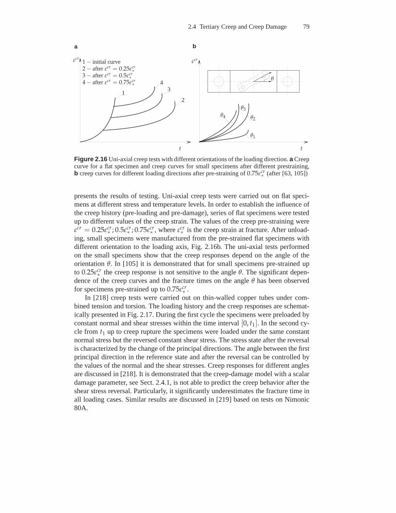
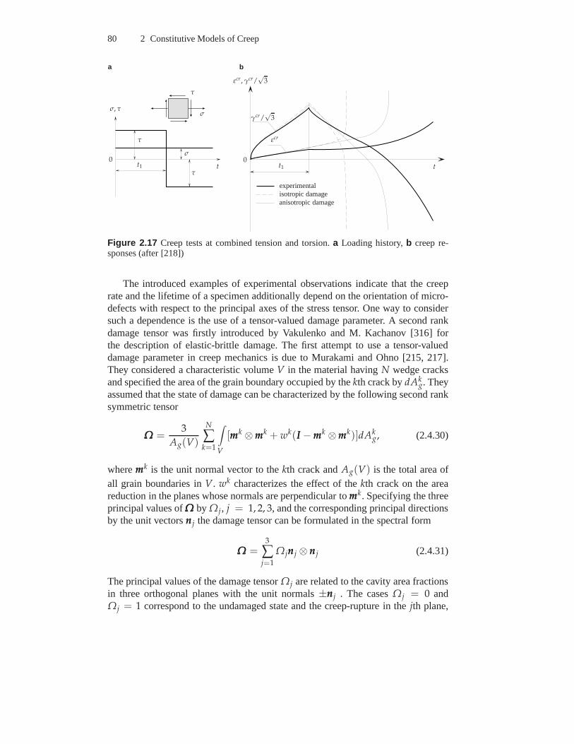
2 Constitutive Models of Creep - ULB Halle: Online … 2 Constitutive Models of Creep Usually, they...

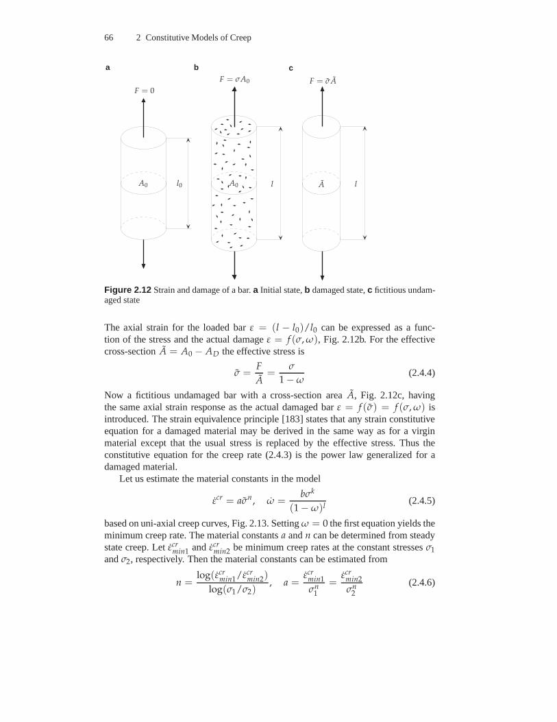
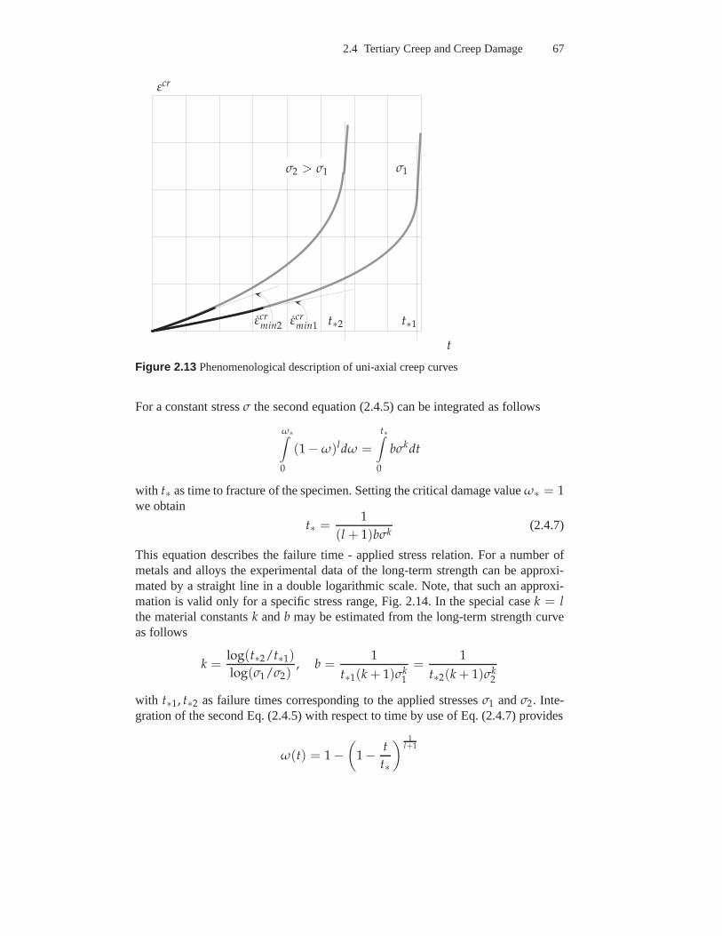
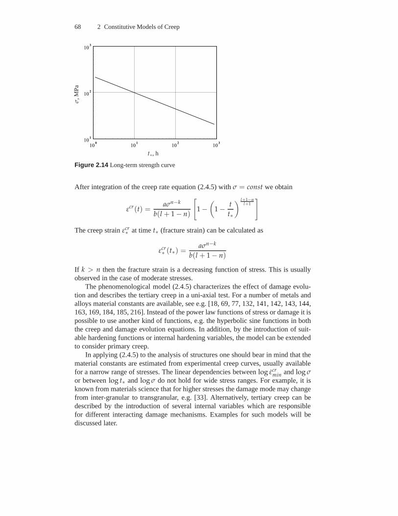
2 Constitutive Models of Creep

Analysis of creep in engineering structures requires the formulation and the solutionof an initial-boundary value problem including the balanceequations and the consti-tutive assumptions. Equations describing the kinematics of three-dimensional solidsas well as balance equations of mechanics of media are presented in monographsand textbooks on continuum mechanics, e.g. [29, 35, 44, 57, 108, 131, 178, 199]. Inwhat follows we discuss constitutive equations for the description of creep behaviorin three-dimensional solids.

The starting point of the engineering creep theory is the introduction of the in-elastic strain, the creep potential, the flow rule, the equivalent stress and internalstate variables, Sect. 2.1. In Sect. 2.2 we discuss constitutive models of secondarycreep. We start with the von Mises-Odqvist creep potential and the flow rule widelyused in the creep mechanics. To account for stress state effects creep potentialsthat include three invariants of the stress tensor are introduced. Consideration ofmaterial symmetries provide restrictions for the creep potential. A novel direct ap-proach to find scalar valued arguments of the creep potentialfor the given group ofmaterial symmetries is proposed. For several cases of material symmetry appropri-ate invariants of the stress tensor, equivalent stress and strain expressions as wellas constitutive equations for anisotropic creep are derived. In Sect. 2.3 we reviewexperimental foundations and models of transient creep behavior under differentmulti-axial loading conditions. Section 2.4 is devoted to the description of tertiarycreep under multi-axial stress states. Various models within the framework of con-tinuum damage mechanics are discussed.

All equations are presented in the direct tensor notation. This notation guaran-tees the invariance with respect to the choice of the coordinate system and has theadvantage of clear and compact representation of constitutive assumptions, partic-ularly in the case of anisotropic creep. The basic rules of the direct tensor calculusas well as some new results for basic sets of invariants with respect to differentsymmetry classes are presented in Appendix A.

2.1 General Remarks

The modeling of creep under multi-axial stress states is thekey step in the adequateprediction of the long-term structural behavior. Such a modeling requires the in-troduction of tensors of stress, strain, strain rate and corresponding inelastic parts.

20 2 Constitutive Models of Creep

Usually, they are discussed within the framework of continuum mechanics start-ing from fundamental balance equations. One of the most important and funda-mental questions is that of the definition (or even the existence) of a measure ofthe inelastic strain and the decomposition of the total strain into elastic and irre-versible parts within the material description. From the theoretical point of viewthis is still a subject of many discussions within the non-linear continuum mechan-ics, e.g. [45, 46, 223, 246].

In engineering mechanics, these concepts are often introduced based on intu-itive assumptions, available experimental data and applications. Therefore, a lot offormulations of multi-axial creep equations can be found inthe literature. In whatfollows some of them will be discussed. First let us recall several assumptions usu-ally made in the creep mechanics [58, 235].

The assumption of infinitesimal strains allows to neglect the difference betweenthe true stresses and strains and the engineering stresses and strains. According tothe continuum mechanics there are no differences between the Eulerian and theLagrangian approaches within the material description. Creep equations in the geo-metrical non-linear case (finite strains) are discussed in the monograph [67], forexample. Finite strain equations based on rheological models are presented in themonographs [175, 246]. The linearized equations of creep continuum mechanicscan be used in the majority of engineering applications because structures are usu-ally designed such that the displacements and strains arising as a consequence of theapplied loading do not exceed the prescribed small values. The exception is the caseof thin-walled shells, where geometrical non-linearitiesmust be considered even ifstrains are infinitesimal, see Sect. 4.4.

The assumption of the classical non-polar continuum restricts the class of mate-rials. The equations of motion within the continuum mechanics include the balanceof momentum and the balance of angular momentum, e.g. [108].These equations in-troduce the stress and the moment stress tensors. Polar materials are those which arecharacterized by constitutive equations with respect to both tensors (in general, theyare non-symmetric). In addition, the rotation degrees of freedom, i.e. the rotationtensor and the angular velocity, are introduced as independent quantities. Models ofpolar media found application to granular or porous materials [97, 104, 214], fibersuspensions [22, 109], or other media with changing microstructure. At present, themoment stress tensor and the anti-symmetric part of the stress tensor are not con-sidered in the engineering creep theories. The reason for this is the higher ordercomplexity of the models and as a consequence increased effort for the identifica-tion of material characteristics.

The assumption of isothermal conditions makes it possible to decouple the ther-mal and the mechanical problem. Furthermore, heat transferproblems are not con-sidered. The influence of the constant temperature on the creep rate is describedby an Arrhenius function, see Sect. 2.2.3. Coupled thermo-mechanical problems ofcreep and damage are discussed in [291], where the influence of creep cavitation onthermal conductivity is considered.

2.1 General Remarks 21

In this chapter we shall use the following notation. Letσσσ be the Cauchy stresstensor andεεε be the tensor of infinitesimal strains as they are defined in [29, 57, 199],among others. Let the symmetric second rank tensorεεεcr be the tensor of the rateof infinitesimal inelastic strains induced by the creep process. For the infinitesimalstrains one can assume the additive split of the total strainrate into elastic and creepparts, i.e.εεε = εεεel + εεεcr. The constitutive equation relating the stress tensor andthe elastic part of the strain tensor can be formulated according to the generalizedHooke’s law [29, 55, 126, 199] and will be introduced later. Creep deformation isaccompanied by various microstructural changes having different influences on thestrain rate. The current state of the material microstructure is determined by theentire previous history of the creep process. It can be characterized by a set of addi-tional field variables termed as internal or hidden state variables. In this chapter weshall discuss internal state variables characterizing thestates of hardening/recoveryand damage. In order to distinguish between the hardening and damage mechanismswe shall specify the “internal hardening variables” byHi and the “internal damagevariables” byωj. The number of such variables and the corresponding evolutionequations (ordinary differential equations with respect to the time variable) is dic-tated by the knowledge of creep-damage mechanisms for a specified metal or alloy,the availability of experimental data on creep and long termstrength as well as thetype of the structural analysis application. In some cases the internal state variablesmust be introduced as tensors of different rank in order to include effects of thedeformation or damage induced anisotropy.

Constitutive equations of multi-axial creep are usually based on the concept ofthe creep potential and the flow rule. The associated flow rulehas the origin in theengineering theory of plasticity. The basic assumptions ofthis theory are:

– The existence of a yield condition (creep condition, see [55], for example) ex-pressed by the equationF(σσσ) = 0, whereF is a scalar valued function. In thegeneral case one can presume thatF depends not only on the stress tensor butalso on the internal state variables and the temperature [202, 265], i.e. the yieldcondition has a form

F(σσσ, Hi, ωj, T) = 0, i = 1, . . . , n, j = 1, . . . , m (2.1.1)

– The existence of a flow potential as a function of the stress tensorΦ(σσσ).

The flow rule (sometimes called the normality rule) is the following assumption forthe inelastic strain rate tensor

εεεin = η∂Φ

∂σσσ, (2.1.2)

whereη is a scalar factor. In the special case that the flow potentialcoincides withthe yield function i.e.Φ = F (2.1.2) represents the associated flow rule. With respectto the variation of the stress tensorδσσσ one distinguishes between the cases of elasticstate, unloading from an elastic-plastic state, neutral loading and loading, i.e.


F(σσσ) < 0, elastic state

F(σσσ) = 0, and δF = δσσσ ······ ∂F

∂σσσ< 0 unloading


∂σσσ= 0 neutral loading


∂σσσ> 0 loading

For work hardening materialsη > 0 is set in the case of loading/neutral loading,otherwiseη = 0, see e.g. [201]. Further details of the flow theory as well as differentarguments leading to (2.1.2) can be found in textbooks on theory of plasticity, e.g.[138, 151, 153, 161, 201, 206, 292].

Within the creep mechanics the flow theory is usually appliedwithout the con-cept of the yield stress or yield condition. This is motivated by the fact that creepis a thermally activated process and the material starts to creep even under low andmoderate stresses lying below the yield limit. Furthermore, at high temperatures0.5Tm < T < 0.7Tm the main creep mechanism for metals and alloys is the dif-fusion of vacancies, e.g. [117]. Under this condition the existence of a yield or acreep limit cannot be verified experimentally. In [185], p.278 it is stated that “theconcept of a loading surface and the loading-unloading criterion which was used inplasticity is no longer necessary”. In monographs [55, 58, 201, 202, 250] the flowrule is applied as follows

εεεcr = η∂Φ

∂σσσ, η > 0 (2.1.3)

Equation (2.1.3) states the “normality” of the creep rate tensor to the surfacesΦ(σσσ) = const. The scalar factorη is determined according to the hypothesis ofthe equivalence of the dissipation power [2, 58]. The dissipation power is definedby P = εεεcr ······ σσσ. It is assumed thatP = εcr

eqσeq, whereεcreq is an equivalent creep

rate andσeq is an equivalent stress. The equivalent measures of stress and creep rateare convenient to compare experimental data under different stress states (see Sect.1.1.2). From the above hypothesis follows

η =P

∂Φ

∂σσσ······ σσσ

=εcr

eqσeq

∂Φ

∂σσσ······ σσσ

(2.1.4)

The equivalent creep rate is defined as a function of the equivalent stress accordingto the experimental data for uni-axial creep as well as creepmechanisms operatingfor the given stress range. An example is the power law stressfunction

εcreq(σeq) = aσn

eq (2.1.5)

Another form of the flow rule without the yield condition has been proposed byOdqvist, [234, 236]. The steady state creep theory by Odqvist, see [234], p.21 isbased on the variational equationδW = δσσσ ······ εεεcr leading to the flow rule

2.1 General Remarks 23

εεεcr =∂W

∂σσσ, (2.1.6)

where the scalar valued functionW(σσσ) plays the role of the creep potential1. In or-der to specify the creep potential, the equivalent stressσeq(σσσ) is introduced. Takinginto account thatW(σσσ) = W(σeq(σσσ)) the flow rule (2.1.6) yields

εεεcr =∂W

∂σeq

∂σeq

∂σσσ= εcr

eq

∂σeq

∂σσσ, εcr

eq ≡∂W

∂σeq(2.1.7)

The creep potentialW(σeq) is defined according to experimental data of creep underuni-axial stress state for the given stress range. An example is the Norton-Bailey-Odqvist creep potential

W =σ0

n + 1

(

σvM

σ0

)n+1

, (2.1.8)

widely used for the description of steady state creep of metals and alloys. In (2.1.8)σ0 andn are material constants andσvM is the von Mises equivalent stress. Belowwe discuss various restrictions on the potentials, e.g. thesymmetries of the creepbehavior and the inelastic incompressibility.

In order to compare the flow rules (2.1.3) and (2.1.6) let us compute the dissipa-tion power. From (2.1.7) it follows

P = εεεcr ······ σσσ =∂W

∂σeq

∂σeq

∂σσσ······ σσσ = εcr

eq

∂σeq

∂σσσ······ σσσ,

We observe that the equivalence of the dissipation power follows from (2.1.7) if theequivalent stress satisfies the following partial differential equation

∂σeq

∂σσσ······ σσσ = σeq (2.1.9)

Furthermore, in this case the flow rules (2.1.3) and (2.1.6) lead to the same creepconstitutive equation. Many proposed equivalent stress expressions satisfy (2.1.9).

The above potential formulations originate from the works of Richard vonMises, where the existence of variational principles is assumed in analogy to thoseknown from the theory of elasticity (the principle of the minimum of the com-plementary elastic energy, for example). Richard von Miseswrote [320]: “DieFormanderung regelt sich derart, daß die pro Zeiteinheit von ihr verzehrte Arbeitunverandert bleibt gegenuber kleinen Variationen der Spannungen innerhalb derFließgrenze. Da die Elastizitatstheorie einen ahnlichen Zusammenhang zwischenden Deformationsgroßen und dem elastischen Potential lehrt, so nenne ich die Span-nungsfunktionF auch das “plastische Potential” oder “Fließpotential”.” It can beshown that the variational principles of linear elasticityare special cases of the en-ergy balance equation (for isothermal or adiabatic processes), see e.g. [198], p. 148,

1 The dependence on the temperature is dropped for the sake of brevity.


for example. Many attempts have been made to prove or to motivate the potentialformulations within the framework of irreversible thermodynamics. For quasi-staticirreversible processes various extremum principles (e.g.the principle of least irre-versible force) are stipulated in [337]. Based on these principles and additional ar-guments like material stability, the potential formulations and the flow rules (2.1.1)and (2.1.6) can be verified. In [185], p. 63 a complementary dissipation potentialas a function of the stress tensor as well as the number of additional forces conju-gate to internal state variables is postulated, whose properties, e.g. the convexity, aresufficient conditions to satisfy the dissipation inequality. In [206] theories of plastic-ity and visco-plasticity are based on the notion of the dissipation pseudo-potentials.However, as far as we know, the flow rules (2.1.1) and (2.1.6) still represent the as-sumptions confirmed by various experimental observations of steady state creep inmetals rather than consequences of the fundamental laws. The advantage of varia-tional statements is that they are convenient for the formulation of initial-boundaryvalue problems and for the numerical analysis of creep in engineering structures.The direct variational methods (for example, the Ritz method, the Galerkin method,the finite element method) can be applied for the numerical solution.

Finally, several creep theories without creep potentials may be found in the lit-erature. In the monograph [246] various constitutive equations of elastic-plastic andelastic-visco-plastic behavior in the sense of rheological models are discussed with-out introducing the plasticity, creep or dissipation potentials. For example, the mod-els of viscous flow of isotropic media known from rheology, e.g. [123, 269], can beformulated as the relations between two coaxial tensors

σσσ = G0III + G1εεε + G2εεε · εεε (2.1.10)

orεεε = H0III + H1σσσ + H2σσσ ··· σσσ, (2.1.11)

whereGi is a function of invariants ofεεε while Hi depend on invariants ofσσσ. Theapplication of the dissipative inequality provides restrictions imposed onGi or Hi.The existence of the potential requires thatGi or Hi must satisfy certain integrabilityconditions [58, 199].

2.2 Secondary Creep 25

2.2 Secondary Creep

Secondary or stationary creep is for many applications the most important creepmodel. After a relatively short transient period the material creeps in such a mannerthat an approximate equilibrium between hardening and softening processes can beassumed. This equilibrium exists for a long time and the long-term behavior of astructure can be analyzed assuming stationary creep processes. In this section sev-eral models of secondary creep are introduced. The secondary or stationary creepassumes constant or slowly varying loading and temperatureconditions. Further-more, the stress tensor is assumed to satisfy the condition of proportional loading,i.e. σσσ(t) = ϕ(t)σσσ0, whereϕ(t) is a slowly varying function of time andσσσ0 is aconstant tensor.

2.2.1 Isotropic Creep

In many cases creep behavior can be assumed to be isotropic. In what follows theclassical potential and the potential formulated in terms of three invariants of thestress tensor are introduced.

2.2.1.1 Classical Creep Equations. The starting point is the Odqvist flow rule(2.1.6). Under the assumption of the isotropic creep, the potential must satisfy thefollowing restriction

W(QQQ ··· σσσ ··· QQQT) = W(σσσ) (2.2.1)

for any symmetry transformationQQQ, QQQ ··· QQQT = III, det QQQ = ±1. From (2.2.1) itfollows that the potential depends only on the three invariants of the stress tensor(see Sect. A.3.1). Applying the principal invariants

J1(σσσ) = tr σσσ, J2(σσσ) =1

2[(tr σσσ)2 − tr σσσ2],

J3(σσσ) = detσσσ =1

6(tr σσσ)3 − 1

2tr σσσtr σσσ2 +

1

3tr σσσ3

(2.2.2)

one can writeW(σσσ) = W(J1, J2, J3)

Any symmetric second rank tensor can be uniquely decomposedinto the sphericalpart and the deviatoric part. For the stress tensor this decomposition can be writtendown as follows

σσσ = σmIII + sss, tr sss = 0 ⇒ σm =1

3tr σσσ,

wheresss is the stress deviator andσm is the mean stress. With the principal invariantsof the stress deviator

J2D = −1

2tr sss2 = −1

2sss ······ sss, J3D =

1

3tr sss3 =

1

3(sss ··· sss) ······ sss


the potential takes the form

W = W(J1, J2D, J3D),

Applying the rule for the derivative of a scalar valued function with respect to asecond rank tensor (see Sect. A.2.4) and (2.1.6) one can obtain

εεεcr =∂W

∂J1III − ∂W

∂J2Dsss +

∂W

∂J3D

(

sss2 − 1

3tr sss2III

)

(2.2.3)

In the classical creep theory it is assumed that the inelastic deformation does notproduce a significant change in volume. The spherical part ofthe creep rate tensoris neglected, i.etr εεεcr = 0. Setting the trace of (2.2.3) to zero results in

tr εεεcr = 3∂W

∂J1= 0 ⇒ W = W(J2D , J3D)

From this follows that the creep behavior is not sensitive tothe hydrostatic stressstateσσσ = −pIII, wherep > 0 is the hydrostatic pressure. The creep equation (2.2.3)can be formulated as

εεεcr = − ∂W

∂J2Dsss +

∂W

∂J3D

(

sss2 − 1

3tr sss2III

)

(2.2.4)

The last term in the right-hand side of (2.2.4) is non-linearwith respect to the stressdeviatorsss. Equations of this type are called tensorial non-linear equations, e.g. [35,58, 202, 265]. They allow to consider some non-classical or second order effects ofthe material behavior [35, 66]. As an example let us considerthe pure shear stressstatesss = τ(mmm ⊗ nnn + nnn ⊗mmm), whereτ is the magnitude of the shear stress andmmmandnnn are orthogonal unit vectors. From (2.2.4) follows

εεεcr = − ∂W

∂J2Dτ(mmm ⊗ nnn + nnn ⊗mmm) +

∂W

∂J3Dτ2

(

1

3III − ppp ⊗ ppp

)

,

where the unit vectorppp is orthogonal to the plane spanned onmmm andnnn. We observethat the pure shear load leads to shear creep rate, and additionally to the axial creeprates (Poynting-Swift effect). Within the engineering creep mechanics such effectsare usually neglected.

The assumption that the potential is a function of the secondinvariant of thestress deviator only, i.e.

W = W(JD2 )

leads to the classical von Mises type potential [320]. In applications it is convenientto introduce the equivalent stress which allows to compare the creep behavior un-der different stress states including the uni-axial tension. The von Mises equivalentstress is defined as follows

σvM =

√

3

2sss ······ sss =

√

−3J2D , (2.2.5)


where the factor3/2 is used for convenience (in the case of the uni-axial tensionwith the stressσ the above expression providesσvM = σ). With W = W(σvM(σσσ))the flow rule (2.1.6) results in

εεεcr =∂W(σvM)

∂σvM

∂σvM

∂σσσ=

∂W(σvM)

∂σvM

3

2

sss

σvM(2.2.6)

The second invariant ofεεεcr can be calculated as follows

εεεcr ······ εεεcr =3

2

[

∂W(σvM)

∂σvM

]2

Introducing the notationε2vM = 2

3 εεεcr ······ εεεcr and taking into account that

P =∂W(σvM)

∂σvMσvM ≥ 0

one can write

εεεcr =3

2εvM

sss

σvM, εvM =

∂W(σvM)

∂σvM(2.2.7)

The constitutive equation of steady state creep (2.2.7) wasproposed by Odqvist[236]. Experimental verifications of this equation can be found, for example, in[295] for steel 45, in [228] for titanium alloy Ti-6Al-4V andin [245] for alloys Al-Si, Fe-Co-V and XC 48. In these works tubular specimens were loaded by tensionforce and torque leading to the plane stress stateσσσ = σnnn ⊗nnn + τ(nnn⊗mmm +mmm ⊗nnn),whereσ andτ are the magnitudes of the normal and shear stresses (see Sect. 1.1.2).Surfacesσ2

vM = σ2 + 3τ2 = const corresponding to the same steady state values ofεvM were recorded. Assuming the Norton-Bailey type potential (2.1.8), from (2.2.7)it follows

εεεcr =3

2aσn−1

vM sss (2.2.8)

This model is widely used in estimations of steady-state creep in structures, e.g.[77, 80, 236, 250, 265].

2.2.1.2 Creep Potentials with Three Invariants of the Stres s Tensor. Insome cases, deviations from the von Mises type equivalent stress were found in ex-periments. For example, different secondary creep rates under tensile and compres-sive loading were observed in [195] for Zircaloy-2, in [106]for aluminium alloyALC101 and in [301], p. 118 for the nickel-based alloy Rene 95. One way to con-sider such effects is to construct the creep potential as a function of three invariantsof the stress tensor. Below we discuss a generalized creep potential, proposed in[9]. This potential leads to tensorial non-linear constitutive equations and allows topredict the stress state dependent creep behavior and second order effects. The 6 un-known parameters in this law can be identified by some basic tests. Creep potentialsformulated in terms of three invariants of the stress tensorare termed non-classical[9].


By analogy to the classical creep equations, the dependenceon the stress tensoris defined by means of the equivalent stressσeq. Various equivalent stress expres-sions have been proposed in the literature for the formulation of yield or failurecriteria, e.g. [27]. In the case of creep, different equivalent stress expressions aresummarized in [160]. In [9] the following equivalent stressis proposed

σeq = ασ1 + βσ2 + γσ3 (2.2.9)

with the linear, the quadratic and the cubic invariants

σ1 = µ1 I1, σ22 = µ2 I2

1 + µ3 I2, σ33 = µ4 I3

1 + µ5 I1 I2 + µ6 I3, (2.2.10)

where Ii = tr σσσi (i = 1, 2, 3) are basic invariants of the stress tensor (see Sect.A.3.1), µj (j = 1, . . . , 6) are parameters, which depend on the material properties.α, β, γ are numerical coefficients for weighting the influence of thedifferent partsin the equivalent stress expression (2.2.9). Such a weighting is usual in phenomeno-logical modelling of material behavior. For example, in [132] similar coefficientsare introduced for characterizing different failure modes.

The von Mises equivalent stress (2.2.5) can be obtained from(2.2.9) by settingα = γ = 0, β = 1 andµ3 = 1.5, µ2 = −0.5. In what follows we setβ = 1 andthe equivalent stress takes the form

σeq = ασ1 + σ2 + γσ3 (2.2.11)

It can be verified that the equivalent stress (2.2.11) satisfies (2.1.9).The flow rule (2.1.6) allows to formulate the constitutive equation for the creep

rate tensor

εεεcr =∂W(σeq)

∂σeq

∂σeq

∂σσσ=

∂W(σeq)

∂σeq

(

α∂σ1

∂σσσ+

∂σ2

∂σσσ+ γ

∂σ3

∂σσσ

)

(2.2.12)

Taking into account the relations between the invariantsσi and the basic invariantsIi and using the rules for the derivatives of the invariants (see Sect. A.2.4), we obtain

∂σ1

∂σσσ= µ1III,

∂σ2

∂σσσ=

µ2 I1III + µ3σσσ

σ2,

∂σ3

∂σσσ=

µ4 I21 III +

µ5

3I2III +

2

3µ5 I1σσσ + µ6σσσ ··· σσσ

σ23

(2.2.13)

As a result, the creep constitutive equation can be formulated as follows

εεεcr =∂W(σeq)

∂σeq

αµ1III+


σ2+γ

(

µ4 I21 +

µ5

3I2

)

III +2


σ23

(2.2.14)Introducing the notation


εcreq ≡

∂W(σeq)

∂σeq

the constitutive equation takes the form

εεεcr = εcreq

αµ1III +


σ2+ γ

(

µ4 I21 +

µ5

3I2

)

III +2


σ23

(2.2.15)Equation (2.2.15) is non-linear with respect to the stress tensor. Therefore, secondorder effects, e.g. [35, 56, 312] are included in the material behavior description. Inaddition, the volumetric creep rate can be calculated from (2.2.15) as follows

εcrV = εcr

eq

[

3αµ1 +(3µ2 + µ3)I1

σ2+ γ

(9µ4 + 2µ5)I21 + 3(µ5 + µ6)I2

3σ23

]

(2.2.16)The volumetric creep rate is different from 0, i.e. the compressibility or dilatationcan be considered.

The derived creep equation has the form (2.1.11) of the general relation betweentwo coaxial tensors. The comparison of (2.1.11) and (2.2.15) provides

H0 = εcreq

(

αµ1 +µ2 I1

σ2+ γ

3µ4 I21 + µ5 I2

3σ23

)

,

H1 = εcreq

(

µ3

σ2+ γ

2µ5 I1

3σ23

)

,

H2 = εcreqγ

µ6

σ23

(2.2.17)

In [9] the power law function of the equivalent stress (2.1.5) is applied to modelcreep behavior of several materials. Four independent creep tests are required toidentify the material constants. The stress states realized in tests should include uni-axial tension, uni-axial compression, torsion and hydrostatic pressure. Let us note,that experimental data which allows to identify the full setof material constants in(2.2.15) are usually not available. In applications one mayconsider the followingspecial cases of (2.2.15) with reduced number of material constants.

The classical creep equation based on the von Mises equivalent stress can bederived assuming the following values of material constants

α = γ = 0, µ2 = −1/2, µ3 = 3/2, (2.2.18)

σeq = σ2 =

√

−1

2I21 +

3

2I2 =

√

3

2sss ······ sss = σvM (2.2.19)

The creep rate tensor takes the form


εεεcr = εcreq

(√

3

2sss ······ sss

)

3σσσ − I1III

2

√

3

2sss ······ sss

=3

2

εcreq(σvM)

σvMsss (2.2.20)

Assuming identical behavior in tension and compression andneglecting secondorder effects fromα = γ = 0, the following equivalent stress can be obtained

σeq = σ2 =√

µ2 I21 + µ3 I2 (2.2.21)

The corresponding creep constitutive equation takes the form

εεεcr = εcreq(σ2)


σ2(2.2.22)

The parametersµ2 and µ3 can be determined from uni-axial tension and torsiontests. Based on the experimental data presented in [165, 166] for technical purecopper M1E (Cu 99,9%) atT = 573 K the parametersµ2 andµ3 are identified in[24].

Neglecting the influence of the third invariant(γ = 0), the creep rate tensor canbe expressed as follows

εεεcr = εcreq(σeq)

(

αµ1III +µ2 I1III + µ3σσσ

σ2

)

(2.2.23)

The above equation describes different behavior in tensionand compression, and in-cludes the volumetric creep rate. Three independent tests,e.g. tension, compressionand torsion are required to identify the material constantsµ1, µ2 andµ3.

With the quadratic invariant and the reduced cubic invariant several special caseswith three material constants can be considered. Setting (αµ1 = µ4 = µ5 = 0) thetensorial non-linear equation can be obtained


(


σ2+ γ

µ6σσσ ··· σσσ

σ23

)

(2.2.24)

With αµ1 = µ4 = µ6 = 0 the creep rate tensor takes the form


(


σ2+ γ

µ5(I2III + 2I1σσσ)

σ23

)

(2.2.25)

The material constants in (2.2.23), (2.2.24) and (2.2.25) were identified in [2, 28]according to data from multi-axial creep tests for plastics(PVC) at room temper-ature [187] and aluminium alloy AK4-1T at 473 K [94, 125, 294]. Furthermore,simulations have been performed in [2, 28] to compare Eqs (2.2.23), (2.2.24) and(2.2.25) as they characterize creep behavior under different loading conditions. Theconclusion was made that cubic invariants applied in (2.2.24) and (2.2.25) do notdeliver any significant improvement in the material behavior description.


2.2.2 Creep of Initially Anisotropic Materials

Anisotropic creep behavior and anisotropic creep modelingare subjects which arerarely discussed in the classical monographs and textbookson creep mechanics(only in some books one may found the flow potentials introduced by von Mises[320] and Hill [138]). The reason for this is that the experimental data from creeptests usually show large scatter within the range of 20% or even more. Therefore,it was often difficult to recognize whether the difference increep curves mea-sured for different specimens (cut from the same material indifferent directions)is the result of the anisotropy. Therefore, it was no use for anisotropic models withhigher order complexity, since the identification of material constants was difficultor even impossible. In the last two decades the importance inmodeling anisotropiccreep behavior of materials and structures is discussed in many publications. In[47, 200, 259, 260, 261, 262] experimental results of creep of superalloys SRR99and CMSX-4 are reported, which demonstrate significant anisotropy of creep be-havior for different orientations of specimens with respect to the crystallographicaxes. In [141] experimental creep curves of a 9CrMoNbV weld metal are presented.They show significant difference for specimens cut in longitudinal (welding) direc-tion and transverse directions. Another example is a material reinforced by fibers,showing quite different creep behavior in direction of fibers and in the transversedirection, e.g. [273, 274].

Within the creep mechanics one usually distinguishes between two kinds ofanisotropy: the initial anisotropy and the deformation or damage induced anisotropy.In what follows the first case will be introduced. The second case will be discussedin Sects 2.3.2 and 2.4.2.

The modeling of anisotropic behavior starts with the concepts of material sym-metry, physical symmetry, symmetry transformation and symmetry group, e.g.[331]. The material symmetry group is related to the symmetries of the materialsmicrostructure, e.g. the crystal symmetries, the symmetries due to the arrangementof fibers in a fiber-reinforced materials, etc. The symmetry transformations are de-scribed by means of orthogonal tensors. Two important of them are

– the reflectionQQQ(nnn) = III − 2nnn ⊗ nnn, (2.2.26)

wherennn is the unit normal to the mirror plane,– the rotation about a fixed axis

QQQ(ϕmmm) = mmm ⊗mmm + cos ϕ(III −mmm ⊗mmm) + sin ϕmmm × III, (2.2.27)

wheremmm is the axis of rotation andϕ (−π < ϕ < π) is the angle of rotation.

Any arbitrary rotation of a rigid body can be described as a composition of three ro-tations (2.2.27) about three fixed axes [333]. Any symmetry transformation can berepresented by means of rotations and reflections, i.e. the tensors of the type (2.2.26)and (2.2.27). The notion of the symmetry group as a set of symmetry transforma-tions was introduced in [230]. The symmetry groups of polar and axial tensors are


discussed in [332]. According to [313], p. 82 a “simple solid” is called aelotropic oranisotropic, if its symmetry group is a proper subgroup of the orthogonal group.

The concept of the “physical symmetry group” is related to the symmetries ofthe material behavior, e.g. linear elasticity, thermal expansion, plasticity, creep, etc.It can only be established based on experimental observations. Physical symmetriesmust be considered in the formulation of constitutive equations and constitutivefunctions. As an example let us consider the symmetry group of the fourth rankelasticity tensor(4)CCC = Cijkleeei ⊗ eeej ⊗ eeek ⊗ eeel as the set of orthogonal tensorsQQQsatisfying the equation, e.g. [25, 332],

(4)CCC′ = CijklQQQ ··· eeei ⊗QQQ ··· eeej ⊗QQQ ··· eeek ⊗QQQ ··· eeel =(4) CCC (2.2.28)

The physical symmetries or the set of orthogonal solutions of (2.2.28) can be foundonly if all the 21 coordinates of the elasticity tensor(4)CCC for a selected basis areidentified from tests. Vice versa, if the physical symmetry group is known then onecan find the general structure of the elasticity tensor basedon (2.2.28). Clearly,neither the elasticity tensor nor the physical symmetry group of the linear elasticbehavior can be exactly found from tests. Establishment of physical symmetries ofcreep behavior is rather complicated due to relatively large scatter of experimentaldata. However, one can relate physical symmetries to the known symmetries of ma-terials microstructure. According to the Neumann principle widely used in differentbranches of physics and continuum mechanics, e.g. [25, 232,332]

The symmetry group of the reason belongs to the symmetry group of theconsequence.

Considering the material symmetries as one of the “reasons”and the physical sym-metries as a “consequence” one can apply the following statement [331]

For a material element and for any of its physical properties every materialsymmetry transformation of the material element is a physical symmetrytransformation of the physical property.

In many cases the material symmetry elements are evident from the arrangementof the materials microstructure as a consequence of manufacturing conditions, forexample. The above principle states that the physical behavior, e.g. the steady statecreep, contains all elements of the material symmetry. The physical symmetry groupusually possesses more elements than the material symmetrygroup, e.g. [232].

2.2.2.1 Classical Creep Equations. Here we discuss steady state creep equa-tions based on the flow rule (2.1.6) and assumption that the creep potential has aquadratic form with respect to the invariants of the stress tensor. These invariantsmust be established according to the assumed symmetry elements of the creep be-havior. The assumption of the quadratic form of the flow potential originates fromthe von Mises work on plasticity of crystals [320]. Therefore, the equations pre-sented below may be termed as von Mises type equations.


Transverse Isotropy. In this case the potentialW(σσσ) must satisfy the followingrestriction

W(QQQ ··· σσσ ···QQQT) = W(σσσ), QQQ(ϕmmm) = mmm ⊗mmm + cos ϕ(III −mmm ⊗mmm) + sin ϕmmm × III(2.2.29)

In (2.2.29)QQQ(ϕmmm) is the assumed element of the symmetry group, wherebymmm isa constant unit vector andϕ is the arbitrary angle of rotation aboutmmm. From therestriction (2.2.29) follows that the potentialW must satisfy the following partialdifferential equation (see Sect. A.3.2)

(mmm × σσσ − σσσ ×mmm) ······(

∂W

∂σσσ

)T

= 0 (2.2.30)

The set of integrals of this equation represent the set of functionally independentscalar valued arguments of the potentialW with respect to the symmetry trans-formation (2.2.29). The characteristic system of (2.2.30)is the system of ordinarydifferential equations

dσσσ

ds= (mmm × σσσ − σσσ ×mmm) (2.2.31)

Any system ofn linear ordinary differential equations has not more thann− 1 func-tionally independent integrals [92]. Sinceσσσ is symmetric, (2.2.31) is a system of sixordinary differential equations and has not more than five functionally independentintegrals. The lists of these integrals are presented by (A.3.15) and (A.3.26). Withinthe classical von Mises type theory second order effects areneglected. Therefore,we have to neglect the arguments which are cubic with respectto the stress tensor.In this case the difference between various kinds of transverse isotropy consideredin Sect. A.3.2 vanishes. It is possible to use different lists of of scalar arguments.The linear and quadratic arguments from (A.3.15) are

tr σσσ, tr σσσ2, mmm ··· σσσ ···mmm, mmm ··· σσσ2 ···mmm (2.2.32)

Instead of (2.2.32) one can use other arguments, for example[273],

tr σσσ, tr sss2 = tr σσσ2 − 1

3(tr σσσ)2,

mmm ··· sss ···mmm = mmm ··· σσσ ···mmm − 1

3tr σσσ,

mmm ··· sss2 ···mmm = mmm ··· σσσ2 ···mmm − 2

3mmm ··· sss ···mmmtr σσσ − 1

9(tr σσσ)2

(2.2.33)

In what follows we prefer another set of invariants which canbe related to (2.2.32)but has a more clear mechanical interpretation. Let us decompose the stress tensoras follows

σσσ = σmmmmm ⊗mmm + σσσp + τττm ⊗mmm + mmm ⊗ τττm (2.2.34)

with the projections


eee2

eee3

eee1

σ11

τ12

σ22

σ33

τ32

τ31

τ13 τ21

τ23

mmm

plane of isotropy

kkk

lll

mmm

σmm

τmk

τml

σkk

σll

τklτlk

τkmτlm

σσσp

Figure 2.1 Stress state in a transversely isotropic medium and corresponding projectionsσmm, σσσp andτττm

σmm = mmm ··· σσσ ···mmm,

σσσp = (III −mmm ⊗mmm) ··· σσσ ··· (III −mmm ⊗mmm),

τττm = mmm ··· σσσ ··· (III −mmm ⊗mmm)

(2.2.35)

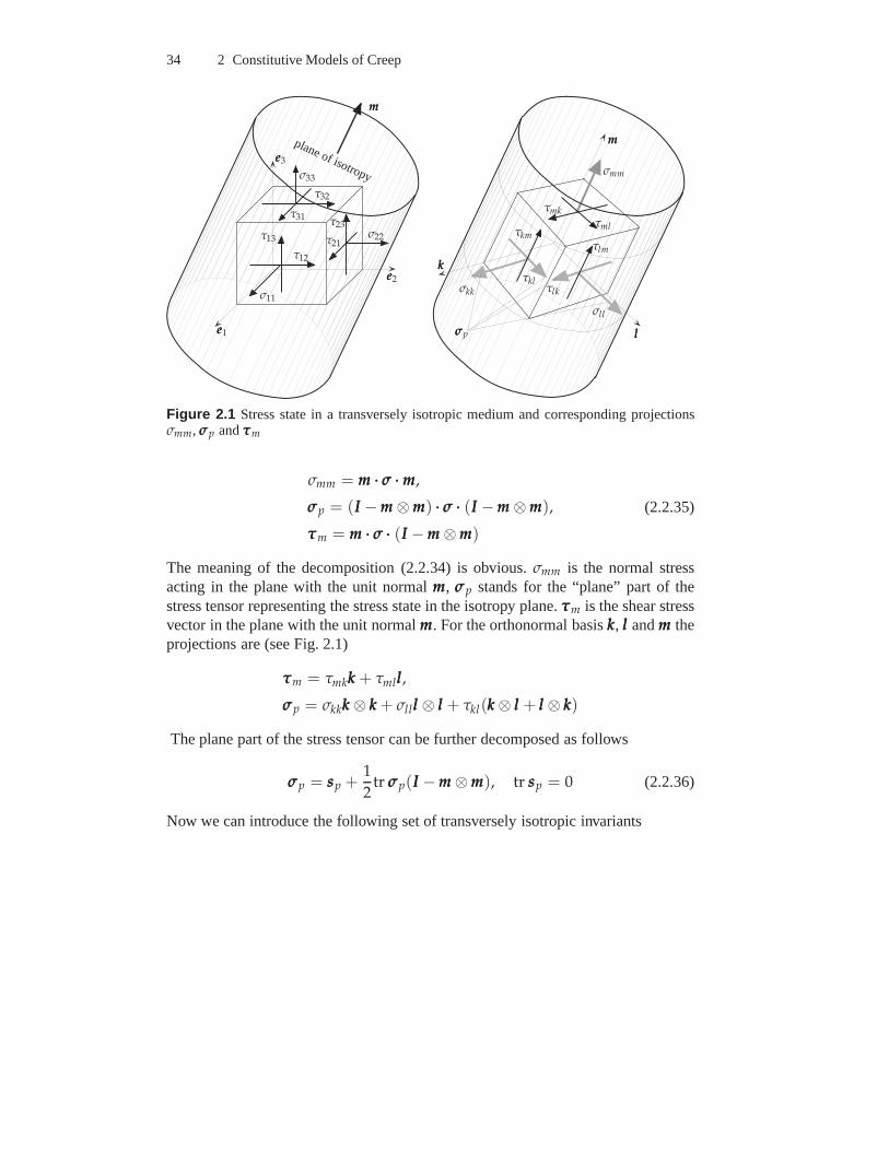
The meaning of the decomposition (2.2.34) is obvious.σmm is the normal stressacting in the plane with the unit normalmmm, σσσp stands for the “plane” part of thestress tensor representing the stress state in the isotropyplane.τττm is the shear stressvector in the plane with the unit normalmmm. For the orthonormal basiskkk, lll andmmm theprojections are (see Fig. 2.1)

τττm = τmkkkk + τmllll,

σσσp = σkkkkk ⊗ kkk + σlllll ⊗ lll + τkl(kkk ⊗ lll + lll ⊗ kkk)

The plane part of the stress tensor can be further decomposedas follows

σσσp = sssp +1

2tr σσσp(III −mmm ⊗mmm), tr sssp = 0 (2.2.36)

Now we can introduce the following set of transversely isotropic invariants


I1m = σmm = mmm ··· σσσ ···mmm,

I2m = tr σσσp = tr σσσ −mmm ··· σσσ ···mmm,

I3m =1

2tr sss2

p =1

2tr σσσ2

p −1

4(tr σσσp)

2

=1

2

(

tr σσσ2 + (mmm ··· σσσ ···mmm)2)

−mmm ··· σσσ2 ···mmm − 1

4(tr σσσ −mmm ··· σσσ ···mmm)2,

I4m = τττm ··· τττm = mmm ··· σσσ2 ···mmm − (mmm ··· σσσ ···mmm)2 = (mmm × σσσ ···mmm) ··· (mmm × σσσ ···mmm)(2.2.37)

In the above listI2m and I3m are two invariants ofσσσp and I4m = τττ2m = τττm ··· τττm

is the square of the length of the shear stress vector acting in the plane with theunit normalmmm. It is shown in Sect. A.3.2 that the above invariants are integrals of(2.2.31).

Taking into account the relations

∂I1m

∂σσσ= mmm ⊗mmm,

∂I2m

∂σσσ= III −mmm ⊗mmm,

∂I3m

∂σσσ= sssp,

∂I4m

∂σσσ= τττmmm ⊗mmm + mmm ⊗ τττmmm

and the flow rule (2.1.6) we obtain the following creep equation

εεεcr =∂W

∂I1mmmm ⊗mmm +

∂W

∂I2m(III −mmm ⊗mmm) +

∂W

∂I3msssp

+∂W

∂I4m(τττmmm ⊗mmm + mmm ⊗ τττmmm)

(2.2.38)

The next assumption of the classical theory is the zero volumetric creep rate. Takingthe trace of (2.2.38) we obtain

tr εεεcr =∂W

∂I1m+ 2

∂W

∂I2m= 0 ⇒ W = W(I1m − 1

2I2m, I3m, I4m) (2.2.39)

Introducing the notation

Jm ≡ I1m − 1

2I2m = mmm ··· σσσ ···mmm − 1

2tr σσσp

the creep equation (2.2.38) takes the form

εεεcr =1

2

∂W

∂Jm(3mmm ⊗mmm − III) +

∂W

∂I3msssp +

∂W

∂I4m(τττmmm ⊗mmm + mmm ⊗ τττmmm) (2.2.40)

By analogy to the isotropic case we formulate the equivalentstress as follows

σ2eq = α1 J2

m + 3α2 I3m + 3α3 I4m

= α1

(

mmm ··· σσσ ···mmm − 1

2tr σσσp

)2

+3

2α2tr sss2

p + 3α3τ2mmm

(2.2.41)


The positive definiteness of the quadratic form (2.2.41) is provided by the conditionsαi > 0, i = 1, 2, 3. The deviatoric partsss of the stress tensor and its second invariantcan be computed by

sss = Jm

(

mmm ⊗mmm − 1

3III

)

+ sssp + τττm ⊗mmm + mmm ⊗ τττm,

tr sss2 =2

3J2m + tr sss2

p + 2τ2mmm

Consequently, the von Mises equivalent stress (2.2.5) follows from (2.2.41) by set-ting α1 = α2 = α3 = 1.

The advantage of the introduced invariants over (2.2.32) or(2.2.33) is that theycan be specified independently from each other. For example,set the second invari-ant in (2.2.32) to zero, i.e.tr σσσ2 = σσσ ······ σσσ = 0. From this follows thatσσσ = 000 andconsequently all other invariants listed in (2.2.32) are simultaneously equal to zero.In addition, the introduced invariants can be related to typical stress states whichshould be realized in creep tests for the identification of constitutive functions andmaterial constants. With the equivalent stress (2.2.41) the creep equation (2.2.40)can be rewritten as follows

εεεcr =3

2σeq

∂W

∂σeq

[

α1 Jm

(

mmm ⊗mmm − 1

3III

)

+ α2sssp + α3(τττm ⊗mmm + mmm ⊗ τττm)

]

(2.2.42)

With the notationεcreq ≡ ∂W

∂σeq(2.2.42) takes the form

εεεcr =3

2

εcreq

σeq

[

α1 Jm

(

mmm ⊗mmm − 1

3III

)

+ α2sssp + α3(τττm ⊗mmm + mmm ⊗ τττm)

]

(2.2.43)

Let us introduce the following parts of the creep rate tensor

εcrmm ≡ mmm ··· εεεcr ···mmm,

εεεcrp ≡ (III −mmm ⊗mmm) ··· εεεcr ··· (III −mmm ⊗mmm),

ǫǫǫcrp ≡ εεεcr

p − 1

2εcr

mm(III −mmm ⊗mmm),

γγγcrm ≡ mmm ··· εεεcr ··· (III −mmm ⊗mmm)

(2.2.44)

From (2.2.42) we obtain

εcrmm = α1

εcreq

σeqJm, ǫǫǫcr

p =3

2α2

εcreq

σeqsssp, γγγcr

m =3

2α3

εcreq

σeqτττm (2.2.45)

Similarly to the isotropic case the equivalent creep rate can be calculated as follows

εcreq =

√

1

α1(εcr

mm)2 +2

3

1

α2ǫǫǫcr

p ······ ǫǫǫcrp +

4

3

1

α3γγγcr

m ··· γγγcrm (2.2.46)


eee2

eee3

eee1

σ11

τ12

σ22

σ33

τ32

τ31

±nnn1±nnn1

±nnn2±nnn2

±nnn3±nnn3

σnnn1nnn1

τnnn1nnn2σnnn2nnn2

σnnn3nnn3

τnnn3nnn2τnnn3nnn1

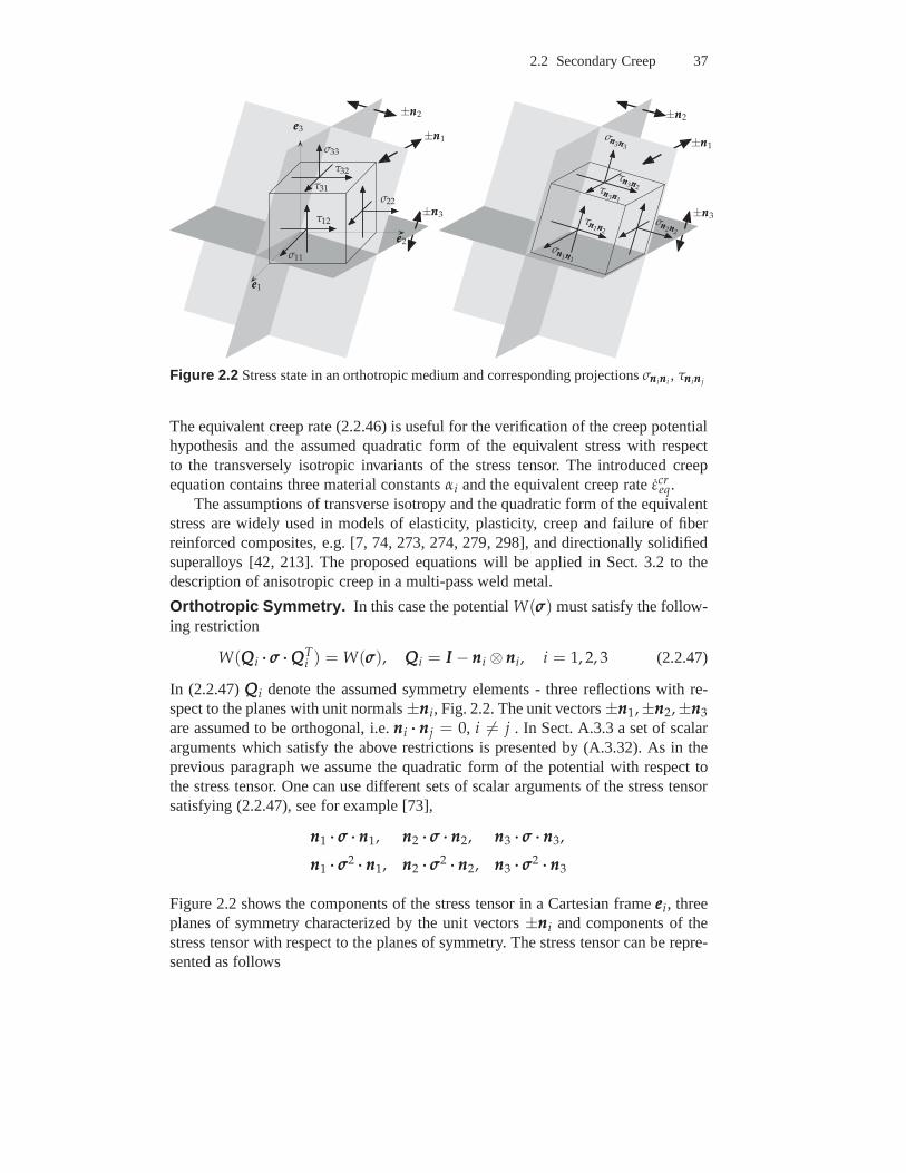
Figure 2.2 Stress state in an orthotropic medium and corresponding projectionsσnnninnni, τnnninnnj

The equivalent creep rate (2.2.46) is useful for the verification of the creep potentialhypothesis and the assumed quadratic form of the equivalentstress with respectto the transversely isotropic invariants of the stress tensor. The introduced creepequation contains three material constantsαi and the equivalent creep rateεcr

eq.The assumptions of transverse isotropy and the quadratic form of the equivalent

stress are widely used in models of elasticity, plasticity,creep and failure of fiberreinforced composites, e.g. [7, 74, 273, 274, 279, 298], anddirectionally solidifiedsuperalloys [42, 213]. The proposed equations will be applied in Sect. 3.2 to thedescription of anisotropic creep in a multi-pass weld metal.

Orthotropic Symmetry. In this case the potentialW(σσσ) must satisfy the follow-ing restriction

W(QQQi ··· σσσ ··· QQQTi ) = W(σσσ), QQQi = III − nnni ⊗ nnni, i = 1, 2, 3 (2.2.47)

In (2.2.47)QQQi denote the assumed symmetry elements - three reflections with re-spect to the planes with unit normals±nnni, Fig. 2.2. The unit vectors±nnn1,±nnn2,±nnn3

are assumed to be orthogonal, i.e.nnni ··· nnnj = 0, i 6= j . In Sect. A.3.3 a set of scalararguments which satisfy the above restrictions is presented by (A.3.32). As in theprevious paragraph we assume the quadratic form of the potential with respect tothe stress tensor. One can use different sets of scalar arguments of the stress tensorsatisfying (2.2.47), see for example [73],

nnn1 ··· σσσ ··· nnn1, nnn2 ··· σσσ ··· nnn2, nnn3 ··· σσσ ··· nnn3,

nnn1 ··· σσσ2 ··· nnn1, nnn2 ··· σσσ2 ··· nnn2, nnn3 ··· σσσ2 ··· nnn3

Figure 2.2 shows the components of the stress tensor in a Cartesian frameeeei, threeplanes of symmetry characterized by the unit vectors±nnni and components of thestress tensor with respect to the planes of symmetry. The stress tensor can be repre-sented as follows


σσσ = σnnn1nnn1nnn1 ⊗ nnn1 + σnnn2nnn2nnn2 ⊗ nnn2 + σnnn3nnn3nnn3 ⊗ nnn3

+ τnnn1nnn2(nnn1 ⊗ nnn2 + nnn2 ⊗ nnn1) + τnnn1nnn3

(nnn1 ⊗ nnn3 + nnn3 ⊗ nnn1)

+ τnnn2nnn3(nnn2 ⊗ nnn3 + nnn3 ⊗ nnn2)

with

σnnn1nnn1= nnn1 ··· σσσ ··· nnn1, σnnn2nnn2 = nnn2 ··· σσσ ··· nnn2, σnnn3nnn3 = nnn3 ··· σσσ ··· nnn3,

τnnn1nnn2 = nnn1 ··· σσσ ··· nnn2, τnnn1nnn3 = nnn1 ··· σσσ ··· nnn3, τnnn2nnn3 = nnn2 ··· σσσ ··· nnn3

According to Sect. A.3.3 we use the following orthotropic invariants of the stresstensor

Innn1nnn1= σnnn1nnn1

, Innn2nnn2 = σnnn2nnn2 , Innn3nnn3 = σnnn3nnn3 ,

Innn1nnn2 = τ2nnn1nnn2

, Innn1nnn3 = τ2nnn1nnn3

, Innn2nnn3 = τ2nnn2nnn3

(2.2.48)

Assuming that the creep potential is a function of six arguments introduced, the flowrule (2.1.6) leads to the following creep equation

εεεcr =∂W

∂Innn1nnn1

nnn1 ⊗ nnn1 +∂W

∂Innn2nnn2

nnn2 ⊗ nnn2 +∂W

∂Innn3nnn3

nnn3 ⊗ nnn3

+∂W

∂Innn1nnn2

nnn1 ··· σσσ ··· nnn2(nnn1 ⊗ nnn2 + nnn2 ⊗ nnn1)

+∂W

∂Innn1nnn3


+∂W

∂Innn2nnn3


(2.2.49)

The assumption of zero volumetric creep rate leads to

tr εεεcr =∂W

∂Innn1nnn1

+∂W

∂Innn2nnn2

+∂W

∂Innn3nnn3

= 0 (2.2.50)

From the partial differential equation (2.2.50) follows that the potentialW is afunction of five scalar arguments of the stress tensor. The characteristic system of(2.2.50) is

dInnn1nnn1

ds= 1,

dInnn2nnn2

ds= 1,

dInnn3nnn3

ds= 1 (2.2.51)

The above system of three ordinary differential equations has two independent inte-grals. One can verify that the following invariants

J1 =1

2(Innn2nnn2 − Innn3nnn3), J2 =

1

2(Innn3nnn3 − Innn1nnn1

), J3 =1

2(Innn1nnn1

− Innn2nnn2)

(2.2.52)are integrals of (2.2.51). Only two of them are independent due to the relationJ1 + J2 + J3 = 0. If the principal directions of the stress tensor coincide with thedirectionsnnni thenτnnninnnj

= 0, i 6= j and the above invariants represent the principalshear stresses. An alternative set of integrals of (2.2.51)is


J1 = Innn1nnn1 −1

3tr σσσ, J2 = Innn2nnn2 −

1

3tr σσσ, J3 = Innn3nnn3 −

1

3tr σσσ (2.2.53)

If the principal directions of the stress tensor coincide with nnni then the above invari-ants are the principal values of the stress deviator. For theformulation of the creeppotential in terms of invariants the relationJ1 + J2 + J3 = 0 must be taken intoaccount.

In what follows we apply the invariants (2.2.52). The equivalent stress can beformulated as follows

σ2eq = 2β1 J2

1 + 2β2 J22 + 2β3 J2

3

+ 3β12 Innn1nnn2 + 3β13 Innn1nnn3 + 3β23 Innn2nnn3

(2.2.54)

The von Mises equivalent stress (2.2.5) follows from (2.2.54) by settingβ1 = β2 =β3 = β12 = β13 = β23 = 1. Applying the flow rule (2.1.6) we obtain the followingcreep equation

εεεcr =εcr

eq

σeq

[

β1 J1(nnn2 ⊗ nnn2 − nnn3 ⊗ nnn3)

+β2 J2(nnn3 ⊗ nnn3 − nnn1 ⊗ nnn1)

+β3 J3(nnn1 ⊗ nnn1 − nnn2 ⊗ nnn2)

+3

2β12τnnn1nnn2(nnn1 ⊗ nnn2 + nnn2 ⊗ nnn1)

+3


+3


]

(2.2.55)

The equivalent stress and the creep equation includes six independent materialconstants. Therefore six independent homogeneous stress states should be realizedin order to identify the whole set of constants. In addition,the dependence of thecreep rate on the equivalent stress must be fitted from the results of uni-axial creeptests for different constant stress values. For example, ifthe power law stress func-tion provides a satisfactory description of steady-state creep then the constantnmust be additionally identified.

An example of orthotropic creep is discussed in [163] for thealuminium alloyD16AT. Plane specimens were removed from rolled sheet alongthree directions:the rolling direction, the transverse direction as well as under the angle of 45 to therolling direction. Uni-axial creep tests were performed at273C and 300C withinthe stress range 63-90 MPa. The results have shown that at 273C creep curvesdepend on the loading direction while at 300C the creep behavior is isotropic.

Other cases. The previous models are based on the assumption of the quadraticform of the creep potential with respect to the stress tensor. The most generalquadratic form can be formulated as follows

σ2eq =

1

2σσσ ······ (4)BBB ······ σσσ, (2.2.56)


whereσeq plays the role of the equivalent stress. The fourth rank tensor (4)BBB mustsatisfy the following restrictions

aaa ······ (4)BBB ······ aaa ≥ 0, aaa ······ (4)BBB = (4)BBB ······ aaa, ccc ······ (4)BBB = 000,

∀ aaa, ccc with aaa = aaaT, ccc = −cccT,(2.2.57)

whereaaa andccc are second rank tensors. Additional restrictions follow from the as-sumed symmetries of the steady state creep behavior. For example, if the orthogonaltensorQQQ stands for a symmetry element, the structure of the tensor(4)BBB can be es-tablished from the following equation

(4)BBB′ = BijklQQQ ··· eeei ⊗QQQ ··· eeej ⊗QQQ ··· eeek ⊗QQQ ··· eeel =(4)BBB, (2.2.58)

whereeeei, i = 1, 2, 3 are basis vectors.The flow rule (2.1.6) provides the following generalized anisotropic creep equa-

tion

εεεcr =εcr

eq

2σeq

(4)BBB ······ σσσ, εcreq ≡ ∂W

∂σeq(2.2.59)

The fourth rank tensors satisfying the restrictions (2.2.57) are well-known fromthe theory of linear elasticity. They are used to represent elastic material proper-ties in the generalized Hooke’s law. The components of thesetensors in a Carte-sian coordinate system are given in the matrix notation in many textbooks on lin-ear elasticity as well as in books and monographs on composite materials, e.g.[6, 7, 29, 122, 256, 309]. Furthermore, different coordinate free representations offourth rank tensors of this type are discussed in the literature. For a review we re-fer to [76]. One of these representations - the projector representation is applied in[47, 48, 200] to constitutive modeling of creep in single crystal alloys under as-sumption of the cubic symmetry.

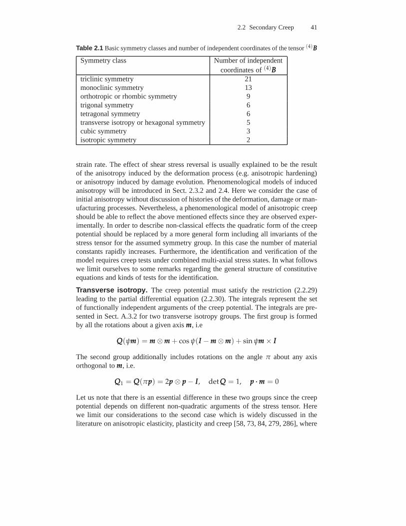
Let us recall that (2.2.59) is the consequence of the creep potential hypothesisand the quadratic form of the equivalent stress with respectto the stress tensor.Similarly to the case of linear elasticity [309] one can prove that only eight basicsymmetry classes are relevant according to these assumptions. The basic symmetryclasses and the corresponding number of independent coordinates of the tensor(4)BBBare listed in Table 2.1. The number of independent coordinates indicates the numberof material constants which should be identified from creep tests. This number canbe reduced if the volume constancy is additionally assumed.For example, in thecases of transverse isotropy and orthotropic symmetry the number of independentcoordinates ofBBB reduces to 3 and 5, respectively (see previous paragraphs).

2.2.2.2 Non-classical Creep Equations. Non-classical effects are the depen-dence of secondary creep rate on the kind of loading and second order effects,see Sect. 2.2.1. Examples of such behavior are different creep rates under ten-sile and compressive stress or the effect of reversal of the shear stress. The lastcase is observed in creep tests on tubular specimens under applied torque. Thechange of the direction of the applied torque leads to different values of the shear


Table 2.1 Basic symmetry classes and number of independent coordinates of the tensor(4)BBB

Symmetry class Number of independentcoordinates of(4)BBB

triclinic symmetry 21monoclinic symmetry 13orthotropic or rhombic symmetry 9trigonal symmetry 6tetragonal symmetry 6transverse isotropy or hexagonal symmetry 5cubic symmetry 3isotropic symmetry 2

strain rate. The effect of shear stress reversal is usually explained to be the resultof the anisotropy induced by the deformation process (e.g. anisotropic hardening)or anisotropy induced by damage evolution. Phenomenological models of inducedanisotropy will be introduced in Sect. 2.3.2 and 2.4. Here weconsider the case ofinitial anisotropy without discussion of histories of the deformation, damage or man-ufacturing processes. Nevertheless, a phenomenological model of anisotropic creepshould be able to reflect the above mentioned effects since they are observed exper-imentally. In order to describe non-classical effects the quadratic form of the creeppotential should be replaced by a more general form including all invariants of thestress tensor for the assumed symmetry group. In this case the number of materialconstants rapidly increases. Furthermore, the identification and verification of themodel requires creep tests under combined multi-axial stress states. In what followswe limit ourselves to some remarks regarding the general structure of constitutiveequations and kinds of tests for the identification.

Transverse isotropy. The creep potential must satisfy the restriction (2.2.29)leading to the partial differential equation (2.2.30). Theintegrals represent the setof functionally independent arguments of the creep potential. The integrals are pre-sented in Sect. A.3.2 for two transverse isotropy groups. The first group is formedby all the rotations about a given axismmm, i.e

QQQ(ψmmm) = mmm ⊗mmm + cos ψ(III −mmm ⊗mmm) + sin ψmmm × III

The second group additionally includes rotations on the angle π about any axisorthogonal tommm, i.e.

QQQ1 = QQQ(πppp) = 2ppp ⊗ ppp − III, det QQQ = 1, ppp ···mmm = 0

Let us note that there is an essential difference in these twogroups since the creeppotential depends on different non-quadratic arguments ofthe stress tensor. Herewe limit our considerations to the second case which is widely discussed in theliterature on anisotropic elasticity, plasticity and creep [58, 73, 84, 279, 286], where


the following invariants are applied2

tr σσσ, tr σσσ2, tr σσσ3, mmm ··· σσσ ···mmm, mmm ··· σσσ2 ···mmm (2.2.60)

To be consistent with derivations in Sect. 2.2.2.1 let us usethe decomposition of thestress tensor (2.2.34) leading to the following set of invariants

I1m = σmm = mmm ··· σσσ ···mmm,

I2m = tr σσσp = tr σσσ −mmm ··· σσσ ···mmm,

I3m =1

2tr sss2

p =1

2tr σσσ2

p −1

4(tr σσσp)

2

=1

2

[

tr σσσ2 + (mmm ··· σσσ ···mmm)2]

−mmm ··· σσσ2 ···mmm − 1

4(tr σσσ −mmm ··· σσσ ···mmm)2,

I4m = τττm ··· τττm = mmm ··· σσσ2 ···mmm − (mmm ··· σσσ ···mmm)2 = (mmm × σσσ ···mmm) ··· (mmm × σσσ ···mmm)

I5m = τττm ··· sssp ··· τττm = mmm ··· σσσ3 ···mmm − 2(mmm ··· σσσ ···mmm)(mmm ··· σσσ2 ···mmm)

+ (mmm ··· σσσ ···mmm)3 − 1

2(tr σσσ −mmm ··· σσσ ···mmm)

[

mmm ··· σσσ2 ···mmm − (mmm ··· σσσ ···mmm)2]

(2.2.61)The meaning of the first four invariants is explained in in Sect. 2.2.2.1. The lastcubic invariant is introduced insteadtr σσσ3. One can prove the following relation

tr σσσ3 = I31m + 3I1m I4m + 3I2m I3m +

3

2I2m I4m +

1

2I32m + 3I5m

Assuming that the creep potentialW is a function of five scalar arguments (2.2.61)and applying the flow rule (2.1.6) we obtain the following creep equation

εεεcr = h1mmm ⊗mmm + (h2−1

2h5 I4m)(III −mmm ⊗mmm) + h3σσσp + h4(τττm ⊗mmm + mmm ⊗ τττm)

+h5

(

τττm ⊗ τττm + mmm ⊗ σσσp ··· τττm + τττm ··· σσσp ⊗mmm)

,(2.2.62)

where

hi =∂W

∂Iim, i = 1, 2, . . . , 5

The last term in the right-hand side of (2.2.62) describes second order effects. Themeaning of these effects is obvious. In the case of non-zero “transverse shear stress”vector

τττm = mmm ··· σσσ ··· (III −mmm ⊗mmm)

the elongation in the direction ofτττm can be considered. The vectorςςςm = sssp ··· τττm

belongs to the isotropy plane, i.e.ςςςm ··· mmm = 0. In the case thatςςςm 6= 000 (2.2.62)describes an additional “transverse shear strain rate” effect.

2 For the description of elastic material behavior instead ofσσσ a strain tensor, e.g. the Cauchy-Green strain tensor is introduced. The five transversely isotropic invariants are the argu-ments of the strain energy density function.


In order to formulate the creep constitutive equation one should specify an ex-pression for the equivalent stress as a function of the introduced invariants. As anexample we present the equivalent stress by use of polynomials of the type (2.2.9)and (2.2.10)

σeq = ασ1 + σ2 + γσ3, (2.2.63)

with

σ1 = µ11 I1m + µ12 I2m,

σ2 = µ21 I21m + µ22 I1m I2m + µ23 I2

2m + µ24 I3m + µ25 I4m,

σ3 = µ31 I31m + µ32 I2

1m I2m + µ33 I1m I22m + µ34 I3

2m + µ35 I1m I3m

+ µ36 I2m I3m + µ37 I1m I4m + µ38 I2m I4m + µ39 I5m

(2.2.64)

The equivalent stress (2.2.63) includes 16 material constants µij and two weight-ing factorsα and γ. The identification of all material constants requires differ-ent independent creep tests under multi-axial stress states. For example, in orderto find the constantµ39 creep tests under stress states with nonzero cubic invari-ant I5m should be carried out. An example is the tension in the isotropy planecombined with the transverse shear stress leading to the stress state of the typeσσσ = σ0nnn1 ⊗ nnn1 + τ0(nnn1 ⊗mmm + mmm ⊗ nnn1), whereσ0 > 0 andτ0 > 0 are the mag-nitudes of the applied stresses,nnn1 is the direction of tension andnnn1 ···mmm = 0. In thiscase

sssp =1

2σ0(nnn1 ⊗ nnn1 − nnn2 ⊗ nnn2), nnn1 ··· nnn2 = 0, τττm = τ0nnn1, I5m =

1

2σ0τ2

0

By analogy to the non-classical models of isotropic creep discussed in Sect.2.2.1 different special cases can be introduced. Settingγ = 0 in (2.2.64), secondorder effects will be neglected. The resulting constitutive model takes into accountdifferent behavior under tension and compression. To find the constantsµ11 andµ12

creep tests under tension (compression) along the direction mmm as well as tension(compression) along any direction in the isotropy plane should be carried out. Set-ting α = 0 the model with the quadratic form of the creep potential with5 constantscan be obtained. The assumption of the zero volumetric creeprate will lead to themodel discussed in Sect. 2.2.2.1.

Second order effects of anisotropic creep were discussed byBetten [52, 58].He found disagreements between creep equations based on thetheory of isotropicfunctions and the creep equation of the type (2.2.62) according to the potential hy-pothesis and the flow rule. The conclusion was made that the potential theory leadsto restrictive forms of constitutive equations if comparedto the representations oftensor functions.

Let us recall the results following from the algebra of isotropic tensor functions[71]. In the case of transverse isotropy group characterized by the symmetry ele-ments (A.3.18) the statement of the problem is to find the general representation ofthe isotropic tensor function of the stress tensorσσσ and the dyadmmm ⊗ mmm (so-called


structure tensor). The constitutive equation describing the creep behavior must befound as follows

εεεcr = fff (σσσ, mmm ⊗mmm),

where fff is an isotropic tensor function of two tensor arguments. Thegeneral repre-sentation of this function is [73]

fff (σσσ, mmm ⊗mmm) = f1mmm ⊗mmm + f2(III −mmm ⊗mmm) + f3σσσ + f4σσσ2

+ f5(mmm ⊗mmm ··· σσσ + σσσ ···mmm ⊗mmm) + f6(mmm ⊗mmm ··· σσσ2+ σσσ2 ···mmm ⊗mmm),(2.2.65)

where the scalarsfi, i = 1, . . . , 6, depend on the five invariants of the stress tensor(2.2.60). Betten found that the last term in (2.2.65) is missing in the constitutiveequation which is based on the potential theory. In order to discuss the meaningof the last term in (2.2.65) let us introduce the identities which follow from thedecomposition of the stress tensor by Eqs (2.2.34) and (2.2.36)

σσσ2 = I2msssp + (I3m +1

4I22m)(III −mmm ⊗mmm) + mmm ⊗ sssp ··· τττm + τττm ··· sssp ⊗mmm

+ (I1m +1

2I2m)(τττm ⊗mmm + mmm ⊗ τττm) + (I2

1m + I4m)mmm ⊗mmm + τττm ⊗ τττm,

(2.2.66)mmm ⊗mmm ··· σσσ + σσσ ···mmm ⊗mmm = τττm ⊗mmm + mmm ⊗ τττm + 2I1mmmm ⊗mmm,

mmm ⊗mmm ··· σσσ2 + σσσ2 ···mmm ⊗mmm = mmm ⊗ sssp ··· τττm + τττm ··· sssp ⊗mmm

+ (I1m +1

2I2m)(τττm⊗mmm + mmm⊗τττm)

+ 2(I4m + I21m)mmm⊗mmm

After inserting (2.2.66), (2.2.34) and (2.2.36) into (2.2.65) we obtain the followingcreep equation

εεεcr = g1mmm ⊗mmm + g2(III −mmm ⊗mmm) + g3sssp + g4(mmm ⊗ τττm + τττm ⊗mmm)

+ g5(mmm ⊗ sssp ··· τττm + τττm ··· sssp ⊗mmm) + g6τττm ⊗ τττm

(2.2.67)with

g1 = f1 + f4(I21m + I4m) + 2 f5 I1m + 2 f6(I4m + I2

1m),

g2 = f2 +1

2f3 I2m + f 4(I3m +

1

4I22m),

g3 = f3 + I2m f4,

g4 = ( f4 + f6)(I1m +1

2I2m) + f5,

g5 = f4 + f6,

g6 = f4


We observe that Eq. (2.2.67) based on the theory of isotropictensor functions doesnot deliver any new second order effect in comparison to (2.2.62). The only dif-ference is that the two last terms in (2.2.67) characterizing the second order ef-fects appear with two different influence functions. The comparison of (2.2.67) with(2.2.62) provides the following conditions for the existence of the potential

∂W

∂I1m= g1,

∂W

∂I2m= g2 +

1

2g5 I4m,

∂W

∂I3m= g3,

∂W

∂I4m= g4,

∂W

∂I5m= g5, g6 = g5

Furthermore, the functionsgi must satisfy the integrability conditions which can beobtained by equating the mixed derivatives of the potentialwith respect to invariants,i.e.

∂2W

∂Iim∂Ikm=

∂2W

∂Ikm∂Iim, i 6= k, i, k = 1, 2, . . . , 5

Let us note that the models (2.2.62) and (2.2.67) are restricted to the special case oftransverse isotropy. In the general case one should analyzethe creep potential withthe invariants listed in (A.3.26).

Other cases. Alternatively a phenomenological constitutive equation of aniso-tropic creep can be formulated with the help of material tensors, e.g. [2]. Introduc-ing three material tensorsAAA, (4)BBB and (6)CCC the equivalent stress (2.2.63) can begeneralized as follows

σeq = ασ1 + σ2 + γσ3 (2.2.68)

with

σ1 = AAA ······ σσσ, σ22 = σσσ ······ (4)BBB ······ σσσ, σ3

3 = σσσ ······ (σσσ ······ (6)CCC ······ σσσ) (2.2.69)

The structure of the material tensors must be established from the following restric-tions

AAA′ = QQQ ··· AAA ···QQQT = AijQQQ ··· eeei ⊗QQQ ··· eeej = AAA,

(4)BBB′ = BijklQQQ ··· eeei ⊗QQQ ··· eeej ⊗QQQ ··· eeek ⊗QQQ ··· eeel =(4)BBB,

(6)CCC′ = CijklmnQQQ ··· eeei ⊗QQQ ··· eeej ⊗QQQ ··· eeek ⊗QQQ ··· eeel ⊗QQQ ··· eeem ⊗QQQ ··· eeen =(6)CCC,(2.2.70)

whereQQQ is an element of the physical symmetry group. The creep potential hypoth-esis and the flow rule (2.1.6) lead to the following creep equation

εεεcr =∂W

∂σeq

(

α∂σ1

∂σσσ+

∂σ2

∂σσσ+ γ

∂σ3

∂σσσ

)

(2.2.71)

Taking into account the relations

∂σ1

∂σσσ= AAA,

∂σ2

∂σσσ=

(4)BBB ······ σσσ

σ2,

∂σ3

∂σσσ=

σσσ ······ (6)CCC ······ σσσ

σ23

(2.2.72)


a generalized anisotropic creep equation can be formulatedas follows

εεεcr = εcreq

(

αAAA +(4)BBB ······ σσσ

σ2+ γ

σσσ ······ (6)CCC ······ σσσ

σ23

)

, εcreq ≡

∂W

∂σeq(2.2.73)

In [51, 265] the following anisotropic creep equation is proposed

εεεcr = HHH + (4)MMM ······ σσσ + ((6)LLL ······ σσσ) ······ σσσ (2.2.74)

Comparing the Eqs (2.2.73) and (2.2.74) the material tensors HHH, (4)MMM and(6)LLL canbe related to the tensorsAAA, (4)BBB and(6)CCC.

The tensorsAAA, (4)BBB and (6)CCC contain 819 coordinates (AAA - 9, (4)BBB - 81, (6)CCC- 729). From the symmetry of the stress tensor and the creep rate tensor as well asfrom the potential hypothesis follows that “only” 83 coordinates are independent (AAA- 6, (4)BBB - 21, (6)CCC - 56). Further reduction is based on the symmetry considerations.The structure of material tensors and the number of independent coordinates can beobtained by solving (2.2.70).

Another possibility of simplification is the establishing of special cases of(2.2.73). For instance, equations with a reduced number of parameters can be de-rived as follows

– α = 1, γ = 0:

σeq = σ1 + σ2, εεεcr = εcreq

(

AAA +(4)BBB ······ σσσ

σ2

)

, (2.2.75)

– α = 0, γ = 1:

σeq = σ2 + σ3, εεεcr = εcreq

(

(4)BBB ······ σσσ

σ2+

σσσ ······ (6)CCC ······ σσσ

σ23

)

, (2.2.76)

– α = 0, γ = 0:

σeq = σ2, εεεcr = εcreq

(

(4)BBB ······ σσσ

σ2

)

(2.2.77)

The last case has been discussed in Sect. 2.2.2.1. Examples of application of con-stitutive equation (2.2.73) as well as different cases of symmetries are discussed in[2, 9].

2.2.3 Functions of Stress and Temperature

In all constitutive equations discussed in Sects 2.2.1 and 2.2.2 the creep potential orthe equivalent creep rate must be specified as functions of the equivalent stress andthe temperature, i.e.

εcreq =

∂W

∂σeq= f (σeq, T)


In [176] the functionf is termed to be the constitutive or response function. For theformulation of constitutive functions one may apply theoretical foundations frommaterials science with regard to mechanisms of creep deformation and related formsof stress and temperature functions. Furthermore, experimental data including fam-ilies of creep curves obtained from uni-axial creep tests for certain ranges of stressand temperature are required. It is convenient to present these families in a formof minimum creep rate vs. stress and minimum creep rate vs. temperature curvesin order to find mechanical properties of the material withinthe steady-state creeprange.

Many empirical functions of stress and temperature which allow to fit exper-imental data have been proposed in the literature, e.g. [236, 250, 266, 292]. Thestarting point is the assumption that the creep rate may be descried as a product oftwo separate functions of stress and temperature

εcreq = fσ(σeq) fT(T)

The widely used functions of stress are:

– power law

fσ(σeq) = ε0

∣

∣

∣

∣

σeq

σ0

∣

∣

∣

∣

n−1 σeq

σ0(2.2.78)

The power law contains three constants (ε0, σ0, n) but only two of them are inde-pendent. Instead ofε0 andσ0 one material constant

a ≡ ε0

σn0

can be introduced.– power law including the creep limit

fσ(σeq) = ε′0

(

σeq

σ′0

− 1

)n′

, σeq > σ′0

If σeq ≤ σ′0 the creep rate is equal zero. In this caseσ′

0 is the assumed creep limit.Let us note that the experimental identification of its valueis difficult, e.g. [266].

– exponential law

fσ(σeq) = ε0 expσeq

σ0

ε0, σ0 are material constants. The disadvantage of this expression is that it predictsa nonzero creep rate for a zero equivalent stress

fσ(0) = ε0 6= 0

– hyperbolic sine law

fσ(σeq) = ε0 sinhσeq

σ0


For low stress values this function provides the linear dependence on the stress

fσ(σeq) ≈ ε0σeq

σ0

Assuming the constant temperature equations for the equivalent creep rate can besummarized as follows

εcreq = aσn

eq Norton, 1929, Bailey, 1929,

εcreq = b

(

expσeq

σ0− 1

)

Soderberg, 1936,

εcreq = a sinh

σeq

σ0Prandtl, 1928, Nadai, 1938, McVetty, 1943,

εcreq = a1σ

n1eq + a2σn2

eq Johnson et al., 1963,

εcreq = a

(

sinhσeq

σ0

)n

Garofalo, 1965,

(2.2.79)

wherea, b, a1, a2, σ0, n, n1 and n2 are material constants. The dependence on thetemperature is usually expressed by the Arrhenius law

fT(T) = exp[−Q/RT],

whereQ andR denote the activation energy and the Boltzmann’s constant,respec-tively.

For the use of stress and temperature functions one should take into accountthat different deformation mechanisms may operate for different specific ranges ofstress and temperature. An overview is provided by the deformation mechanismsmaps proposed by Frost and Ashby [117], Fig. 2.3. Contours ofconstant strain ratesare presented as functions of the normalized equivalent stressσeq/G and the ho-mologous temperatureT/Tm, whereG is the shear modulus andTm is the meltingtemperature. For a given combination of the stress and the temperature, the mapprovides the dominant creep mechanism and the strain rate.

Let us briefly discuss different regions on the map, the mechanisms of creepdeformation and constitutive functions derived in materials science. For compre-hensive reviews one may consult [116, 156, 222]. The originsof the inelastic de-formation at the temperature range0.5 < T/Tm < 0.7 are transport processesassociated with motion and interaction of dislocations anddiffusion of vacancies.Here we limit our consideration to the two classes of physical models - dislocationand diffusion creep. Various creep rate equations within the dislocation creep rangeare based on the Bailey-Orowan recovery hypothesis. An internal barrier stressσint

being opposed to the dislocation movement is assumed. When the plastic strain oc-curs the internal stress increases as a result of work hardening due to accumulationof deformation and due to increase of the dislocation density. As the material is sub-jected to the load and temperature over certain time, the internal stressσint recovers.In the uni-axial case the rate of change of the internal stress is assumed as follows


0 0.2 0.4 0.6 0.8 1.0

10−6

10−5

10−4

10−3

10−2

10−1

Plasticity

Diffusional Flow

(Grain Boundary) (Lattice)

Ela

stic

ity

Power-law Creep

T/Tm

σeq

/G

10−6/s

L.T.Creep H.T.Creep

Figure 2.3 Schematic deformation-mechanism map (L.T.Creep - low temperature creep,H.T.Creep - high temperature creep)

σint = hεcr − rσint,

whereh andr are material properties related to hardening and recovery,respectively.In the steady stateσint = 0 so that

εcr =rσint

h

Specifying the values forr, h andσint various models for the steady state creep ratehave been derived. An example is the following expression (for details of derivationwe refer to [116])

εcr ∝D

RT

σ4

G3exp

(

− Q

RT

)

,

whereD is the diffusion coefficient.Further models of dislocation creep are discussed under theassumption of

the climb-plus-glide deformation mechanism. At high temperatures and moderatestresses, dislocations can climb as well as glide. The glideof dislocations producedby the applied stress is opposed by obstacles. Due to diffusion of vacancies, the


dislocations can climb around strengthening particles. The inelastic strain is thencontrolled by the glide, while its rate is determined by the climb. The climb-plus-glide mechanism can be related to the recovery-hardening hypothesis. The harden-ing results from the resistance to glide due to interaction of moving dislocationswith other dislocations, precipitates, etc. The recovery mechanism is the diffusioncontrolled climb which releases the glide barriers. The climb-plus-glide based creeprate models can be found in [116, 117, 222]. The common resultis the power-lawcreep

εcreq ∝

(σeq

G

)nexp

(

− Q

RT

)

(2.2.80)

Equation (2.2.80) can be used to fit experimental data for a range of stresses upto 10−3G. The exponentn varies from 3 to about 10 for metallic materials. Athigher stresses above10−3G the power law (2.2.80) breaks down. The measuredstrain rate is greater than the Eq. (2.2.80) predicts. Within the range of the power-law break down a transition from the climb-plus-glide to theglide mechanism isassumed [117]. The following empirical equation can be applied, e.g. [117, 222],

εcreq ∝

[

sinh(

ασeq

G

)]nexp

(

− Q

RT

)

, (2.2.81)

whereα is a material constant. Ifασeq/G < 1 then (2.2.81) reduces to (2.2.80).At higher temperatures (T/Tm > 0.7) diffusion mechanisms control the creep

rate. The deformation occurs at much lower stresses and results from diffusion ofvacancies. The mechanism of grain boundary diffusion (Coble creep) assumes dif-fusive transport of vacancies through and around the surfaces of grains. The devi-atoric part of the stress tensor changes the chemical potential of atoms at the grainboundaries. Because of different orientations of grain boundaries a potential gra-dient occurs. This gradient is the driving force for the grain boundary diffusion.The diffusion through the matrix (bulk diffusion) is the dominant creep mechanism(Nabarro-Herring creep) for temperatures close to the melting point. For details con-cerning the Coble and the Nabarro-Herring creep models we refer to [116, 222].These models predict the diffusion controlled creep rate tobe a linear function ofthe stress.

In addition to the dislocation and the diffusion creep, the grain boundary slidingis the important mechanism for poly-crystalline materials. This mechanism occursbecause the grain boundaries are weaker than the ordered crystalline structure ofthe grains [222, 271]. Furthermore, the formation of voids and micro-cracks ongrain boundaries contributes to the sliding. The whole deformation rate depends onthe grain size and the grain aspect ratio (ratio of the grain dimensions parallel andperpendicular to the tensile stress direction). Samples with a larger grain size usuallyexhibit a lower strain rate.

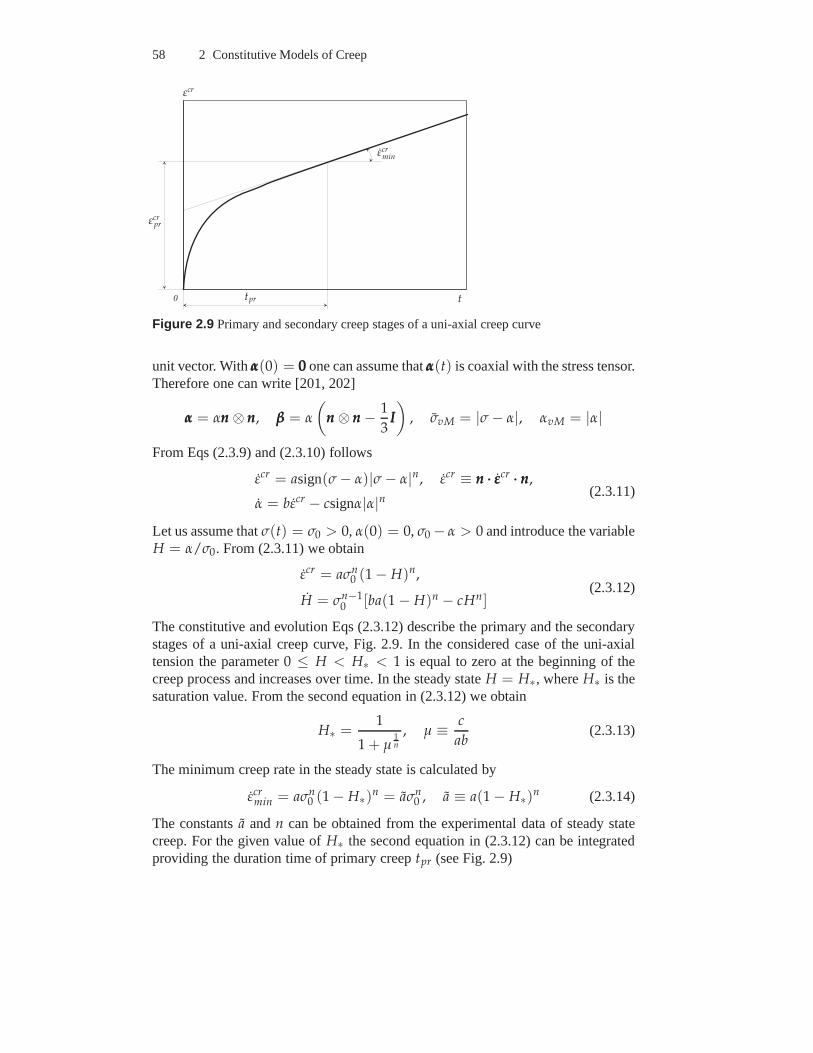
2.3 Primary Creep and Creep Transients 51

2.3 Primary Creep and Creep Transients

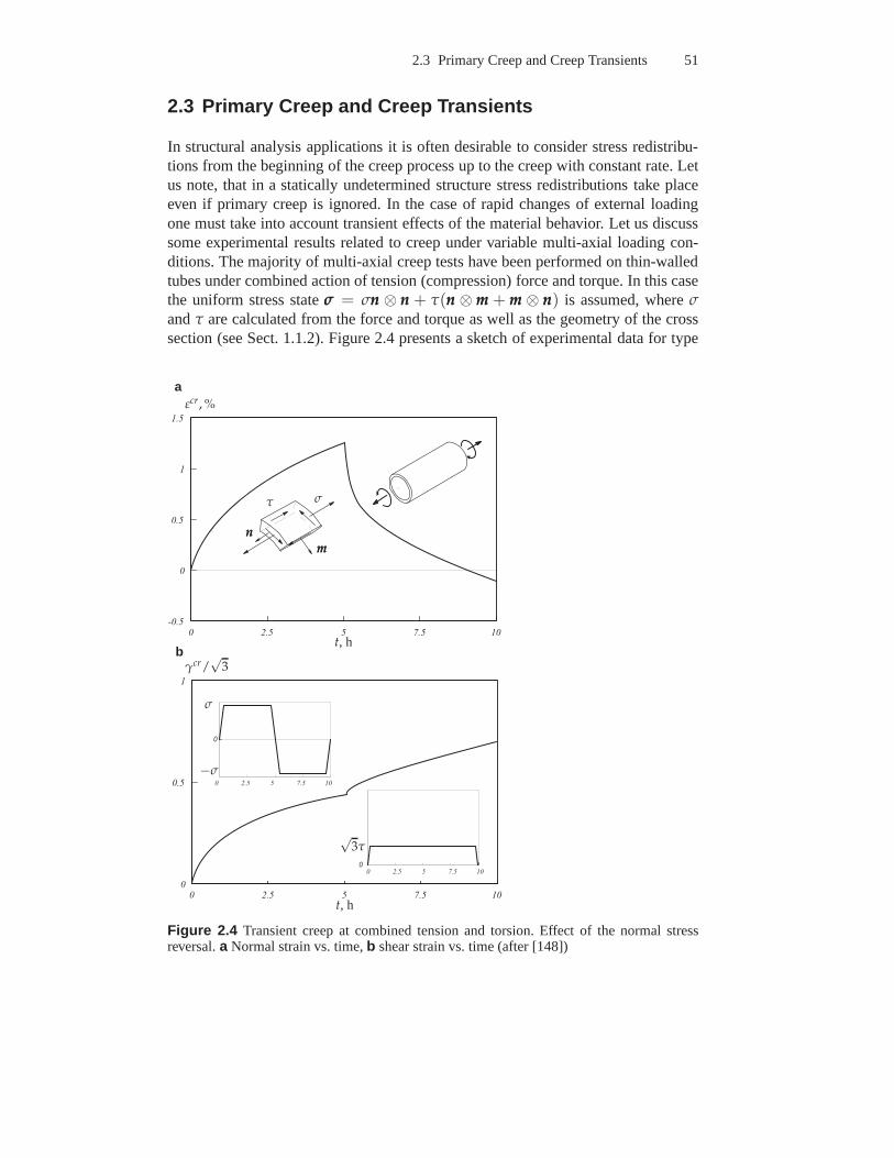
In structural analysis applications it is often desirable to consider stress redistribu-tions from the beginning of the creep process up to the creep with constant rate. Letus note, that in a statically undetermined structure stressredistributions take placeeven if primary creep is ignored. In the case of rapid changesof external loadingone must take into account transient effects of the materialbehavior. Let us discusssome experimental results related to creep under variable multi-axial loading con-ditions. The majority of multi-axial creep tests have been performed on thin-walledtubes under combined action of tension (compression) forceand torque. In this casethe uniform stress stateσσσ = σnnn ⊗ nnn + τ(nnn ⊗ mmm + mmm ⊗ nnn) is assumed, whereσandτ are calculated from the force and torque as well as the geometry of the crosssection (see Sect. 1.1.2). Figure 2.4 presents a sketch of experimental data for type

0 2 . 5 5 7 . 5 1 0- 0 . 5

0

0 . 5

1

1 . 5

0 2 . 5 5 7 . 5 1 00

0 . 5

1

0 2 . 5 5 7 . 5 1 0

0

0 2 . 5 5 7 . 5 1 00

t, h

t, h

εcr, %

γcr/√

3

σ

σ

−σ

√3τ

τ

nnnmmm

a

b

Figure 2.4 Transient creep at combined tension and torsion. Effect of the normal stressreversal.a Normal strain vs. time,b shear strain vs. time (after [148])


0 1 0 0 2 0 0 3 0 0 4 0 0 5 0 0- 0 . 4

- 0 . 2

0

0 . 2

0 . 4

0 . 6

0 . 8

1

0 1 0 0 2 0 0 3 0 0 4 0 0 5 0 0

0

t, h

γcr, %

τ

−τ

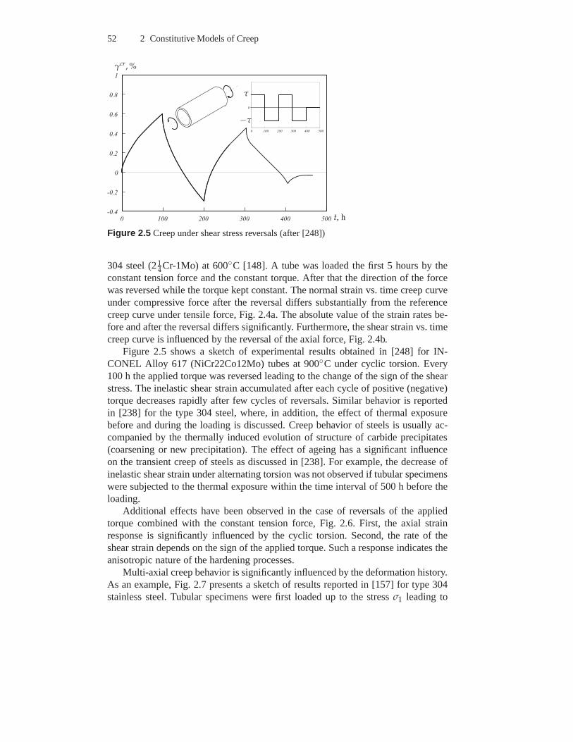
Figure 2.5 Creep under shear stress reversals (after [248])

304 steel (214Cr-1Mo) at 600C [148]. A tube was loaded the first 5 hours by theconstant tension force and the constant torque. After that the direction of the forcewas reversed while the torque kept constant. The normal strain vs. time creep curveunder compressive force after the reversal differs substantially from the referencecreep curve under tensile force, Fig. 2.4a. The absolute value of the strain rates be-fore and after the reversal differs significantly. Furthermore, the shear strain vs. timecreep curve is influenced by the reversal of the axial force, Fig. 2.4b.

Figure 2.5 shows a sketch of experimental results obtained in [248] for IN-CONEL Alloy 617 (NiCr22Co12Mo) tubes at 900C under cyclic torsion. Every100 h the applied torque was reversed leading to the change ofthe sign of the shearstress. The inelastic shear strain accumulated after each cycle of positive (negative)torque decreases rapidly after few cycles of reversals. Similar behavior is reportedin [238] for the type 304 steel, where, in addition, the effect of thermal exposurebefore and during the loading is discussed. Creep behavior of steels is usually ac-companied by the thermally induced evolution of structure of carbide precipitates(coarsening or new precipitation). The effect of ageing hasa significant influenceon the transient creep of steels as discussed in [238]. For example, the decrease ofinelastic shear strain under alternating torsion was not observed if tubular specimenswere subjected to the thermal exposure within the time interval of 500 h before theloading.

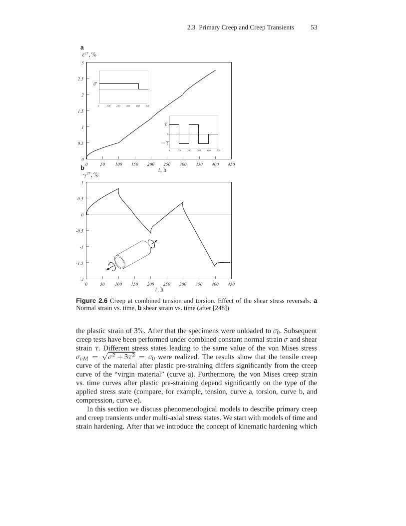
Additional effects have been observed in the case of reversals of the appliedtorque combined with the constant tension force, Fig. 2.6. First, the axial strainresponse is significantly influenced by the cyclic torsion. Second, the rate of theshear strain depends on the sign of the applied torque. Such aresponse indicates theanisotropic nature of the hardening processes.

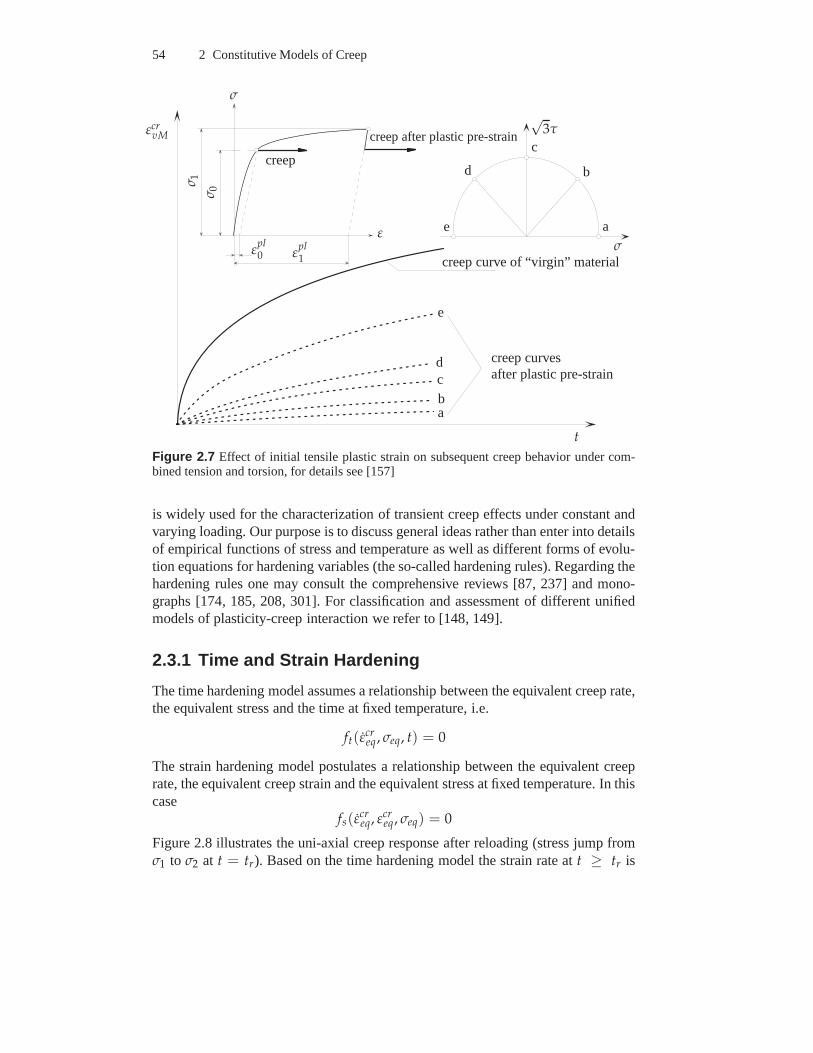
Multi-axial creep behavior is significantly influenced by the deformation history.As an example, Fig. 2.7 presents a sketch of results reportedin [157] for type 304stainless steel. Tubular specimens were first loaded up to the stressσ1 leading to


0 5 0 1 0 0 1 5 0 2 0 0 2 5 0 3 0 0 3 5 0 4 0 0 4 5 0- 2

- 1 . 5

- 1

- 0 . 5

0

0 . 5

1

0 5 0 1 0 0 1 5 0 2 0 0 2 5 0 3 0 0 3 5 0 4 0 0 4 5 00

0 . 5

1

1 . 5

2

2 . 5

3

0 1 0 0 2 0 0 3 0 0 4 0 0 5 0 0

0 1 0 0 2 0 0 3 0 0 4 0 0 5 0 0

0

t, h

t, h

εcr, %

γcr, %

τ

−τ

σ

a

b

Figure 2.6 Creep at combined tension and torsion. Effect of the shear stress reversals.aNormal strain vs. time,b shear strain vs. time (after [248])

the plastic strain of3%. After that the specimens were unloaded toσ0. Subsequentcreep tests have been performed under combined constant normal strainσ and shearstrain τ. Different stress states leading to the same value of the vonMises stressσvM =

√σ2 + 3τ2 = σ0 were realized. The results show that the tensile creep

curve of the material after plastic pre-straining differs significantly from the creepcurve of the “virgin material” (curve a). Furthermore, the von Mises creep strainvs. time curves after plastic pre-straining depend significantly on the type of theapplied stress state (compare, for example, tension, curvea, torsion, curve b, andcompression, curve e).

In this section we discuss phenomenological models to describe primary creepand creep transients under multi-axial stress states. We start with models of time andstrain hardening. After that we introduce the concept of kinematic hardening which


t

εcrvM

ε

σ

εpl0 ε

pl1

σ 0

σ 1

creep

creep after plastic pre-strain

creep curve of “virgin” material

creep curvesafter plastic pre-strain

σ

√3τ

a

a

b

b

c

c

d

d

e

e

Figure 2.7 Effect of initial tensile plastic strain on subsequent creep behavior under com-bined tension and torsion, for details see [157]

is widely used for the characterization of transient creep effects under constant andvarying loading. Our purpose is to discuss general ideas rather than enter into detailsof empirical functions of stress and temperature as well as different forms of evolu-tion equations for hardening variables (the so-called hardening rules). Regarding thehardening rules one may consult the comprehensive reviews [87, 237] and mono-graphs [174, 185, 208, 301]. For classification and assessment of different unifiedmodels of plasticity-creep interaction we refer to [148, 149].

2.3.1 Time and Strain Hardening

The time hardening model assumes a relationship between theequivalent creep rate,the equivalent stress and the time at fixed temperature, i.e.

ft(εcreq, σeq, t) = 0

The strain hardening model postulates a relationship between the equivalent creeprate, the equivalent creep strain and the equivalent stressat fixed temperature. In thiscase

fs(εcreq, εcr

eq, σeq) = 0

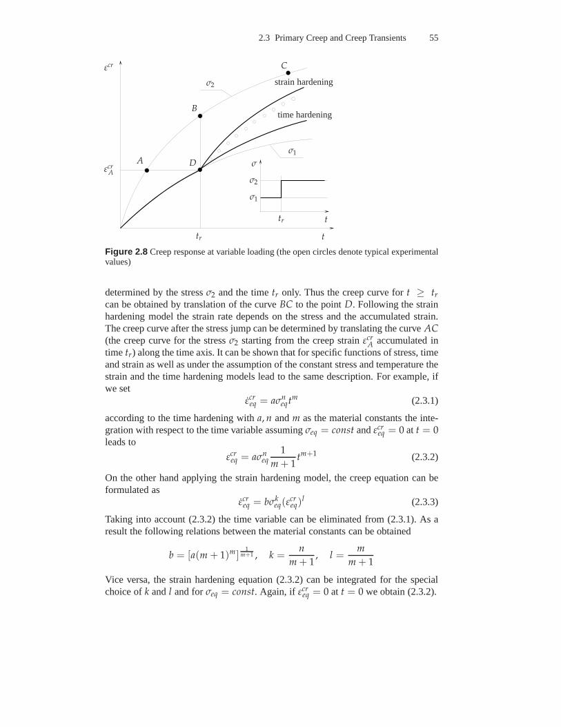
Figure 2.8 illustrates the uni-axial creep response after reloading (stress jump fromσ1 to σ2 at t = tr). Based on the time hardening model the strain rate att ≥ tr is


replacements

t

t

εcr

A

B

C

tr

tr

εcrA

σ

σ1

σ2

time hardening

strain hardening

σ1

σ2

D

Figure 2.8 Creep response at variable loading (the open circles denotetypical experimentalvalues)

determined by the stressσ2 and the timetr only. Thus the creep curve fort ≥ tr

can be obtained by translation of the curveBC to the pointD. Following the strainhardening model the strain rate depends on the stress and theaccumulated strain.The creep curve after the stress jump can be determined by translating the curveAC(the creep curve for the stressσ2 starting from the creep strainεcr

A accumulated intime tr) along the time axis. It can be shown that for specific functions of stress, timeand strain as well as under the assumption of the constant stress and temperature thestrain and the time hardening models lead to the same description. For example, ifwe set

εcreq = aσn

eqtm (2.3.1)

according to the time hardening witha, n andm as the material constants the inte-gration with respect to the time variable assumingσeq = const andεcr

eq = 0 at t = 0leads to

εcreq = aσn

eq1

m + 1tm+1 (2.3.2)

On the other hand applying the strain hardening model, the creep equation can beformulated as

εcreq = bσk

eq(εcreq)

l (2.3.3)

Taking into account (2.3.2) the time variable can be eliminated from (2.3.1). As aresult the following relations between the material constants can be obtained

b = [a(m + 1)m]1

m+1 , k =n

m + 1, l =

m

m + 1

Vice versa, the strain hardening equation (2.3.2) can be integrated for the specialchoice ofk andl and forσeq = const. Again, if εcr

eq = 0 at t = 0 we obtain (2.3.2).


Applying the time hardening model the von Mises-Odqvist creep theory (seeSect. 2.2) can be generalized as follows

εεεcr =3

2aσn−1

vM tmsss (2.3.4)

By analogy one can formulate the creep constitutive equation with the strain hard-ening

εεεcr =3

2bσk−1

vM (εcrvM)lsss (2.3.5)

The time and the strain hardening models provide simple empirical descriptionof the uni-axial creep curve within the range of primary creep and are still popularin characterizing the material behavior, e.g. [137, 145, 171]. Despite the simplicity,both the models suffer from significant limitations, even ifapplied stress and tem-perature are constant. The disadvantage of the time hardening model is that the timevariable appears explicitly in equation (2.3.1) for the creep rate. An additional draw-back is that the constantsm andl take usually the values−1 < m < 0, −1 < l < 0as the result of curve fitting. Ifεcr

eq = 0 at t = 0 then Eq. (2.3.3) provides an infinitestarting creep rate. One can avoid this problem in a time-step based numerical pro-cedure assuming a small non-zero creep equivalent strain atthe starting time step.Finally, both models can be applied only for the case of the constant or slowly vary-ing stresses. Transient creep effects under rapid changes of loading and particularlyin the case of stress reversals cannot be described.

Further details of time and strain hardening models can be found in [173, 250].In [173] a modified strain hardening model is proposed based on the idea of creepstrain origins.

2.3.2 Kinematic Hardening

The common approach in describing transient creep effects under complex loadingpaths is the introduction of internal state variables and appropriate evolution equa-tions (the so-called hardening rules). The scalar-valued internal state variables areintroduced in the literature to characterize isotropic hardening and ageing processes.An example will be discussed in Sect. 2.4.1.3. Several “non-classical” effects ob-served in tests under non-proportional loading have motivated the use of tensor-valued variables (usually second rank tensors).

The idea of kinematic hardening (translation of the yield surface in the stressspace) originates from the theory of plasticity and has beenintroduced by Prager[257]. In the creep mechanics the kinematic hardening was proposed by Malininand Khadjinsky [203, 204]. The starting point is the additive decomposition of thestress tensor into two parts:σσσ = σσσ + ααα, whereσσσ is called the active or the effectivepart of the stress tensor andααα denotes the additional or translation part of the stresstensor (back stress tensor). The introduced tensors can be further decomposed intospherical and deviatoric parts


σσσ =1

3tr σσσIII + sss, tr sss = 0,

ααα =1

3tr αααIII + βββ, tr βββ = 0,

σσσ =1

3(tr σσσ + tr ααα)III + sss, sss = sss + βββ

(2.3.6)

It is assumed that the inelastic strain rate is determined bythe active part of the stresstensor. The creep potential is then a function of the active part of the stress tensor, i.e.W = W(σσσ) = W(σσσ − ααα), e.g. [245]. As in the case of the classical isotropic creep(Sect. 2.2.1.1) only the second invariant of the deviatorsss is considered. Introducingthe von Mises equivalent stress

σvM ≡√

3

2sss ······ sss =

√

3

2(sss − βββ) ······ (sss − βββ) (2.3.7)

the flow rule (2.1.6) leads to the following constitutive equation

εεεcr =3

2

εcrvM

σvMsss, εvM ≡

√

2

3εεεcr ······ εεεcr (2.3.8)

The equivalent creep rate can be expressed by the use of stress and temperaturefunctions discussed in Sect. 2.2.3. For example, with the power law stress functionand the Arrhenius temperature dependence

εcrvM = aσn

vM, a = a0 exp

(

− Q

RT

)

(2.3.9)

Equations (2.3.8) contain the deviatoric part of the back stressβββ. This internal statevariable is defined by the evolution equation and the initialcondition. In [201, 202]the following evolution equation is postulated

βββ =2

3bεεεcr − g(αvM)

αvMβββ (2.3.10)

with

αvM ≡√

3

2βββ ······ βββ

For the functiong various empirical relations were proposed. One example is [201,202]

g(αvM) = cαnvM, c = c0 exp

(

− Qr

RT

)

Equation (2.3.10) is the multi-axial utilization of the Bailey-Orowan recovery hy-pothesis, see Sect. 2.2.3.b and c0 are material constants andQr is the activationenergy of recovery.

Let us show how the model behaves for the uni-axial homogeneous stress stateσσσ(t) = σ(t)nnn ⊗ nnn, whereσ(t) is the magnitude of the applied stress andnnn is the


0 t

εcr

tpr

εcrpr

εcrmin

Figure 2.9 Primary and secondary creep stages of a uni-axial creep curve

unit vector. Withααα(0) = 000 one can assume thatααα(t) is coaxial with the stress tensor.Therefore one can write [201, 202]

ααα = αnnn ⊗ nnn, βββ = α

(

nnn ⊗ nnn − 1

3III

)

, σvM = |σ − α|, αvM = |α|

From Eqs (2.3.9) and (2.3.10) follows

εcr = asign(σ − α)|σ − α|n, εcr ≡ nnn ··· εεεcr ··· nnn,

α = bεcr − csignα|α|n(2.3.11)

Let us assume thatσ(t) = σ0 > 0, α(0) = 0, σ0 − α > 0 and introduce the variableH = α/σ0. From (2.3.11) we obtain

εcr = aσn0 (1 − H)n,

H = σn−10 [ba(1 − H)n − cHn]

(2.3.12)

The constitutive and evolution Eqs (2.3.12) describe the primary and the secondarystages of a uni-axial creep curve, Fig. 2.9. In the considered case of the uni-axialtension the parameter0 ≤ H < H∗ < 1 is equal to zero at the beginning of thecreep process and increases over time. In the steady stateH = H∗, whereH∗ is thesaturation value. From the second equation in (2.3.12) we obtain

H∗ =1

1 + µ1n

, µ ≡ c

ab(2.3.13)

The minimum creep rate in the steady state is calculated by

εcrmin = aσn

0 (1 − H∗)n = aσn0 , a ≡ a(1 − H∗)n (2.3.14)

The constantsa andn can be obtained from the experimental data of steady statecreep. For the given value ofH∗ the second equation in (2.3.12) can be integratedproviding the duration time of primary creeptpr (see Fig. 2.9)


0 2 4 6 8 1 00

0 . 0 5

0 . 1

0 . 1 5

0 . 2

0 . 2 5

0 . 3

0 . 3 5

0 2 4 6 8 1 00

0 . 1

0 . 2

0 . 3

0 . 4

0 . 5

0 . 6

0 . 7

0 . 8

0 2 4 6 8 1 0

0

t/tprt/tpr

εcr/[a(1 − H∗)σn0 tpr] H

σ0

a b

Figure 2.10 Uni-axial creep after unloading. Simulations based on Eqs (2.3.15) for the casen = 3 andH∗ = 0.7. a Creep strain vs. time,b hardening variable vs. time.

tpr =ϕ(H∗)baσn

0

, ϕ(H∗) =

H∗∫

0

dH

(1 − H)n − µHn

From the first equation in (2.3.12) the creep strainεcrpr follows at t = tpr (see Fig.

2.9) as

εcrpr =

σ0

b

H∗∫

0

(1 − H)ndH

(1 − H)n − µHn

The above equations can be used for the identification of material constants.To discuss the model predictions for the case of the uni-axial cyclic loading let

us introduce the following dimensionless variables

σ =σ(t)

σ0, τ =

t

tpr, ǫ =

εcr

a(1 − H∗)σn0 tpr

,

where σ0 denotes the constant stress value in the first loading cycle.Equations(2.3.11) take the form

dǫ

dτ= asign(σ − H)

|σ − H|n1 − H∗ ,

dH

dτ= ϕ(H∗)

[

sign(σ − H)|σ − H|n − sign(H)

(

1 − H∗H∗

)n

|H|n]

(2.3.15)Figures 2.10 and 2.11 illustrate the results of the numerical integration of (2.3.15)with n = 3, H∗ = 0.7 and the initial conditionsǫ(0) = 0 andH(0) = 0. In the firstcase presented in Fig. 2.10 we assumeσ = σ0 within the time interval[0, 2tpr ], sothat the hardening variable increases up to the saturation value and remains constant.The creep curve exhibits both the primary and the secondary stages, Fig. 2.10b. Att = 2tpr we assume a spontaneous unloading, i.e.σ = 0. We observe that the model


0 1 2 3 4 5 6- 0 . 2

- 0 . 1

0

0 . 1

0 . 2

0 . 3

0 . 4

0 1 2 3 4 5 6- 0 . 8

- 0 . 6

- 0 . 4

- 0 . 2

0

0 . 2

0 . 4

0 . 6

0 . 8

0 2 4 6

0

t/tprt/tpr

εcr/[a(1 − H∗)σn0 tpr] H

σ0

σ0

a b

Figure 2.11 Uni-axial creep under cyclic loading. Simulations based onEqs (2.3.15) for thecasen = 3 andH∗ = 0.7. a Creep strain vs. time,b hardening variable vs. time.

(2.3.15) is able to describe the creep recovery (see Fig. 1.3b). Figure 2.11 presentsthe numerical results for the case of cyclic loading. Three loading cycles with theconstant stresses±σ0 and the holding time∆t = 2tpr, Fig. 2.11a, are considered.We observe that the model (2.3.15) predicts identical creepresponses for the firstand the third loading cycle.

Let us give some comments on the model predictions under multi-axial stressstates. For this purpose we consider the case that the stressdeviatorsss is the knownconstant tensor within a given interval of time[t0, t]. Equations (2.3.8) and (2.3.10)can be rewritten as follows

εεεcr =3

2

f (σvM)

σvM(sss − βββ),

βββ = bf (σvM)

σvM(sss − βββ)− g(αvM)

αvMβββ

(2.3.16)

In the steady creep stateβββ = βββ∗, whereβββ∗ is the saturation value of the back stressdeviator. From the second equation in (2.3.16) it follows

bf (σvM∗ )

σvM∗(sss − βββ∗) =

g(αvM∗)

αvM∗βββ∗, (2.3.17)

where

σvM∗ =

√

3

2(sss − βββ∗) ······ (sss − βββ∗), αvM∗ =

√

3

2βββ∗ ······ βββ∗

The double inner product of (2.3.17) with itself results in

[b f (σvM∗ )]2 = [g(αvM∗ )]

2

Since f (σvM∗) > 0 andg(αvM∗) > 0 we obtain

b f (σvM∗) = g(αvM∗) (2.3.18)


From (2.3.17) it follows

βββ∗ =αvM∗

σvM∗ + αvM∗sss ⇒ σvM∗ = σvM + αvM∗ (2.3.19)

Now the steady state value of the back stress deviator can be calculated

βββ∗ = αvM∗sss

σvM(2.3.20)

Let us assume power functions forf andg. Then from (2.3.18) it follows

ba(σvM − αvM∗)n = cαn

vM∗

As in the uni-axial case we introduce the hardening variableH = αvM/σvM. Thesaturation valueH∗ is then determined by (2.3.13). From the first Eq. in (2.3.16)weobtain

εεεcrst =

3

2aσn−1

vm sss, a ≡ a(1 − H∗)n (2.3.21)

We observe that the kinematic hardening model (2.3.16) results in the classicalNorton-Bailey-Odqvist constitutive equation of steady-state creep discussed in Sect.2.2.1. This model predicts isotropic steady state creep independently from the initialcondition for the back stress deviatorβββ. Furthermore, different stress states leadingto the same value of the von Mises equivalent stress will provide the same steadystate value of the equivalent creep rate.

The model (2.3.16) is applied in [202, 245] for the description of creep for dif-ferent materials under simple or non-proportional loadingconditions. It is demon-strated that the predictions agree with experimental results. However, in many casesdeviations from the Norton-Bailey-Odqvist type steady state creep can be observedin experiments. For example, in the case shown in Fig. 2.6 thesteady state shearcreep rate changes significantly after the shear stress reversals, although the vonMises equivalent stress remains constant. The results presented in Fig. 2.7 indicatethat the initial hardening state due to plastic pre-strain is the reason for the stressstate dependence of the subsequent creep behavior. This effect cannot be describedby the model (2.3.16).

The models with the back stress of the type (2.3.16) are usually termed to bethe models with anisotropic hardening, e.g. [202]. The typeof anisotropy is thendetermined by the symmetry group of the back stress tensor ordeviator. The sym-metry group of any symmetric second rank tensor includes always nine elements,e.g. [199]. For the tensorβββ the symmetry elements are

QQQβββ = ±nnn1 ⊗ nnn1 ± nnn2 ⊗ nnn2 ± nnn3 ⊗ nnn3, (2.3.22)

wherennni are the principal axes. In order to verify the assumed symmetries of hard-ening one should perform creep tests with non-proportionalloading of the followingtype. During the first cycle a homogeneous constant stress state with the deviatoricpartsss should be applied over a period of time[0, t1], t1 < tpr. During the second


loading cycle the stress statesQQQi ··· sss ··· QQQTi should be applied, where the orthogonal

tensorsQQQi do not belong to the symmetry group ofsss. Among all stress states of thistype the stress statesQQQβββ ··· sss ··· QQQT

βββ should exist leading to the same (with respect tothe scatter of experimental data) creep response after reloading.

As shown in [72] kinematic hardening of the type (2.3.16) leads to a restrictiveform of orthotropic inelastic behavior. In order to demonstrate this let us write downthe back stress deviator in the following form

βββ = β1nnn1 ⊗ nnn1 + β2nnn2 ⊗ nnn2 − (β1 + β2)nnn3 ⊗ nnn3

= β1(nnn1 ⊗ nnn1 − nnn3 ⊗ nnn3) + β2(nnn2 ⊗ nnn2 − nnn3 ⊗ nnn3),

whereβ1 andβ2 are the principal values andnnn1, nnn2 andnnn3 are the principal direc-tions ofβββ. For the given back stress deviatorβββ the equivalent stress (2.3.7) takes theform

σ2vM = 3 J2

1

(

1 − β1

J1

)2

+ 3 J22

(

1 − β2

J2

)2

+3

2J1 J2

(

1 − β1

J1

)(

1 − β2

J2

)

+ 3I2nnn1nnn2

+ 3I2nnn1nnn3

+ 3I2nnn2nnn3

,(2.3.23)

where the invariantsJi are defined by Eqs (2.2.53) and the invariantsInnninnnjare defined

by Eqs (2.2.48). Steady state creep with initial orthotropic symmetry is discussed inSect. 2.2.2. In this case the von Mises type equivalent stress includes 6 invariantsand 6 independent material constants. The equivalent stress (2.3.23) contains all6 orthotropic invariants. However, the last three terms (three shear stresses withrespect to the three planes of the orthotropic symmetry) arenot affected by thehardening. Furthermore, in the steady state range these terms vanish since the backstress deviatorβββ∗ is coaxial with the stress deviator according to (2.3.20).

The possibilities to improve the predictions of the kinematic hardening modelare:

– Introduction of additional state variables like isotropichardening variable, e.g.[87], ageing variable, e.g. [238], or damage variables, e.g. [101]. Models withdamage variables will be discussed in Sect. 2.4.

– Formulation of the creep potential as a general isotropic function of two tensorsσσσandααα. Such an approach is proposed in [72] for the case of plasticity and includesdifferent special cases of kinematic hardening,

– Consideration of the initial anisotropy of the material behavior, e.g. [148].

Creep models with kinematic hardening of the type (2.3.8) and different specificforms of the hardening evolution equation are discussed in [158, 159, 202, 238, 245,272] among others. For the description of creep and creep-plasticity interaction atcomplex loading conditions a variety of unified models is available including thehardening variables as second rank tensors. For details we refer to [174, 176, 185,208]. Several unified models are reviewed and evaluated in [148, 149]. The historicalbackground of the development of non-linear kinematic hardening rules is presentedin [87].

2.4 Tertiary Creep and Creep Damage 63

2.4 Tertiary Creep and Creep Damage

Tertiary creep stage is the final part of the creep process. Ina uni-axial creep curvetertiary creep is observed as the increase of the creep rate.The shape of the finalpart of the creep curve and the duration of the tertiary creepdepends on the materialcomposition, the stress level and the temperature. For somestructural steels, thetertiary creep is the major part of the whole creep process, e.g. [105, 242].

The origins of tertiary creep are progressive damage processes including theformation, growth and coalescence of voids on grain boundaries, coarsening of pre-cipitates and environmental effects. The voids may nucleate earlier during the creepprocess, possibly at primary creep stage or even after spontaneous deformation. Theinitially existing micro-defects have negligible influence on the creep rate. As theirnumber and size increase with time, they weaken the materialproviding the de-crease in the load-bearing capacity. The coalescence of cavities or propagation ofmicro-cracks lead to the final fracture. Creep fracture is usually inter-granular [33].Dyson [99] distinguishes three main categories of creep damage: the strain induceddamage, the thermally induced damage and the environmentally induced damage.The strain induced damage may be classified as follows [101]

– excessive straining at constant load,– grain boundary cavitation and– progressive multiplication of the dislocation substructure

The first two damage mechanisms occur in all poly-crystalline materials, whereasthe third one is essential for nickel-based super-alloys.

The thermally induced damage mechanisms include material ageing processeswhich lead to the loss of strength and contribute to the nucleation and growth ofcavities. The example of the thermally induced ageing includes the coarsening ofcarbide precipitates for ferritic steels (increase of volume fraction of carbide precip-itates or new precipitation), e.g. [251]. The rate of ageingdoes not depend on theapplied stress, but is influenced by the temperature and can be identified by exposingtest-pieces to thermal environment.

The environmentally induced damage (corrosion, oxidation, etc.) appears dueto the attack of chemical species contained within the surrounding medium. Theenvironmental damage rate can be inversely related to the test-piece (component)dimensions [99].

The dominance of a creep damage mechanism depends on the alloy composi-tion, on the fabrication route and on the service conditions. For several metals andalloys, fracture mechanism maps are available [33]. By analogy with the deforma-tion mechanism maps, regions with different fracture modesare indicated dependingon the stress and the temperature ranges.

Physical modeling of creep damage is complicated by the factthat many differ-ent mechanisms may operate and interact in a specific material under given loadingconditions. This interaction should be taken into account in the damage rate equa-tions. Models related to the grain boundary cavitation are discussed and reviewed in[155, 271].


The characterization of tertiary creep under multi-axial stress states is the im-portant step in a creep analysis of engineering structures.A lifetime prediction of aspecific load bearing component designed for creep, or a residual lifetime estima-tion of a structure operating at elevated temperature requires a model which takesinto account tertiary creep and damage evolution under multi-axial stress states.

The damage rate and consequently the creep rate are determined by the stresslevel, the accumulated damage and the temperature. These dependencies can be es-tablished based on experimental data from the uni-axial creep testing. If the materialis subjected to multi-axial loading, the kind of stress state has a significant influenceon the damage growth. Tension and compression lead to different creep rates. Dif-ferent stress states corresponding to the same von Mises equivalent stress lead, ingeneral, to different equivalent tertiary creep rates while the equivalent strain rate inthe secondary stage is approximately the same. These facts are established from thedata of creep tests under combined tension and torsion, e.g.[169, 170], as well asfrom biaxial and triaxial creep tests [282, 283]. Stress state effects must be consid-ered in the damage evolution equation. In Sect. 2.4.1 we discuss various possibilitiesto characterize the tertiary creep behavior by means of scalar valued damage para-meters. Under non-proportional loading conditions, the additional factor is the in-fluence of the damage induced anisotropy. Examples are creeptests under combinedtension and alternating torsion, e.g. [218], and creep tests under biaxial loading withalternating direction of the first principal stress [283]. In both cases the assumptionof isotropic creep behavior and the scalar measure of damagelead to disagreementwith experimental observations. In Sect. 2.4.2 we review some experimental resultsillustrating the damage induced anisotropy and discuss creep-damage models withtensor-valued damage variables.

2.4.1 Scalar-Valued Damage Variables

Many microstructural observations show the directional effect of creep damage. Forexample, during a cyclic torsion test on copper voids nucleate and grow predomi-nantly on those grain boundaries, which are perpendicular to the first principal di-rection of the stress tensor, e.g. [134]. Creep damage has therefore an anisotropicnature and should be characterized by a tensor. However, if the initially isotropicmaterial is subjected to constant or monotonic loading the influence of the damageanisotropy on the observed creep behavior, i.e. the strain vs. time curves, is not sig-nificant. If the state of damage is characterized by a tensor (see Sect. 2.4.2) then sucha tensor can be assumed to be coaxial with the stress tensor under monotonic loadingconditions. In such a case only the scalar damage measures will enter the creep con-stitutive equation. Below we introduce different models oftertiary creep includingthe phenomenological, the so-called micromechanically consistent and mechanismbased models. The effect of damage is described by means of scalar valued damageparameters and corresponding evolution equations. The stress state influences areexpressed in the equivalent stress responsible for the damage evolution.2.4.1.1 Kachanov-Rabotnov Model. The phenomenological creep-damageequations were firstly proposed by L. Kachanov [150] and Rabotnov [263]. A new


internal variable has been introduced to characterize the “continuity” or the “dam-age” of the material. The geometrical interpretation of thecontinuity variable startsfrom changes in the cross-section area of a uni-axial specimen. Specifying the initialcross-section area of a specimen byA0 and the area of voids, cavities, micro-cracks,etc. byAD, the Kachanov’s continuity is defined as follows (see [152])

ψ =A0 − AD

A0

The valueψ = 1 means the virgin, fully undamaged state, the conditionψ = 0corresponds to the fracture (completely damaged cross-section).

Rabotnov [263, 264, 265] introduced the dual damage variable ω. In [264] hepointed out that the damage state variableω “may be associated with the area frac-tion of cracks, but such an interpretation is connected witha rough scheme and istherefore not necessary”. Rabotnov assumed that the creep rate is additionally de-pendent on the current damage state. The constitutive equation should have the form

εcr = εcr(σ, ω)

Furthermore, the damage processes can be reflected in the evolution equation

ω = ω(σ, ω), ω|t=0 = 0, ω < ω∗,

whereω∗ is the critical value of the damage parameter for which the material fails.With the power functions of stress and damage the constitutive equation may beformulated as follows

εcr =aσn

(1 − ω)m(2.4.1)

Similarly, the damage rate can be expressed by

ω =bσk

(1 − ω)l(2.4.2)

These equations contain the material dependent constants:a, b, n, m, l, k. It is easyto prove that for the damage free state (ω = 0), the first equation results in thepower law creep constitutive equation.

Settingm = n the first equation can be written as

εcr = aσn, (2.4.3)

where σ = σ/(1 − ω) is the so-called net-stress or effective stress. In this case(2.4.3) is a generalization of the Norton-Bailey secondarycreep law for the descrip-tion of tertiary creep process. Lemaitre and Chaboche [185]proposed the effectivestress concept to formulate constitutive equations for damaged materials based onavailable constitutive equation for “virgin” materials. An interpretation can be givenfor a tension bar, Fig. 2.12. HereA0 denotes the initial cross-section area of the bar,Fig. 2.12a. From the given tensile forceF the stress can be computed asσ = F/A0.


F = 0

A0 l0

F = σA0

A0

F = σA

A ll

a b c

Figure 2.12 Strain and damage of a bar.a Initial state,b damaged state,c fictitious undam-aged state

The axial strain for the loaded barε = (l − l0)/l0 can be expressed as a func-tion of the stress and the actual damageε = f (σ, ω), Fig. 2.12b. For the effectivecross-sectionA = A0 − AD the effective stress is

σ =F

A=

σ

1 − ω(2.4.4)

Now a fictitious undamaged bar with a cross-section areaA, Fig. 2.12c, havingthe same axial strain response as the actual damaged barε = f (σ) = f (σ, ω) isintroduced. The strain equivalence principle [183] statesthat any strain constitutiveequation for a damaged material may be derived in the same wayas for a virginmaterial except that the usual stress is replaced by the effective stress. Thus theconstitutive equation for the creep rate (2.4.3) is the power law generalized for adamaged material.

Let us estimate the material constants in the model

εcr = aσn, ω =bσk

(1 − ω)l(2.4.5)

based on uni-axial creep curves, Fig. 2.13. Settingω = 0 the first equation yields theminimum creep rate. The material constantsa andn can be determined from steadystate creep. Letεcr

min1 and εcrmin2 be minimum creep rates at the constant stressesσ1

andσ2, respectively. Then the material constants can be estimated from

n =log(εcr

min1/εcrmin2)

log(σ1/σ2), a =

εcrmin1

σn1

=εcr

min2

σn2

(2.4.6)


t

t∗2 t∗1εcrmin2 εcr

min1

σ1σ2 > σ1

εcr

Figure 2.13 Phenomenological description of uni-axial creep curves

For a constant stressσ the second equation (2.4.5) can be integrated as follows

ω∗∫

0

(1 − ω)ldω =

t∗∫

0

bσkdt

with t∗ as time to fracture of the specimen. Setting the critical damage valueω∗ = 1we obtain

t∗ =1

(l + 1)bσk(2.4.7)

This equation describes the failure time - applied stress relation. For a number ofmetals and alloys the experimental data of the long-term strength can be approxi-mated by a straight line in a double logarithmic scale. Note,that such an approxi-mation is valid only for a specific stress range, Fig. 2.14. Inthe special casek = lthe material constantsk andb may be estimated from the long-term strength curveas follows

k =log(t∗2/t∗1)

log(σ1/σ2), b =

1

t∗1(k + 1)σk1

=1

t∗2(k + 1)σk2

with t∗1, t∗2 as failure times corresponding to the applied stressesσ1 andσ2. Inte-gration of the second Eq. (2.4.5) with respect to time by use of Eq. (2.4.7) provides

ω(t) = 1 −(

1 − t

t∗

) 1l+1


100

101

102

103

101

102

103

t∗, h

σ,M

Pa

Figure 2.14 Long-term strength curve

After integration of the creep rate equation (2.4.5) withσ = const we obtain

εcr(t) =aσn−k

b(l + 1 − n)

[

1 −(

1 − t

t∗

) l+1−nl+1

]

The creep strainεcr∗ at timet∗ (fracture strain) can be calculated as

εcr∗ (t∗) =

aσn−k

b(l + 1 − n)

If k > n then the fracture strain is a decreasing function of stress.This is usuallyobserved in the case of moderate stresses.

The phenomenological model (2.4.5) characterizes the effect of damage evolu-tion and describes the tertiary creep in a uni-axial test. For a number of metals andalloys material constants are available, see e.g. [18, 69, 77, 132, 141, 142, 143, 144,163, 169, 184, 185, 216]. Instead of the power law functions of stress or damage it ispossible to use another kind of functions, e.g. the hyperbolic sine functions in boththe creep and damage evolution equations. In addition, by the introduction of suit-able hardening functions or internal hardening variables,the model can be extendedto consider primary creep.

In applying (2.4.5) to the analysis of structures one shouldbear in mind that thematerial constants are estimated from experimental creep curves, usually availablefor a narrow range of stresses. The linear dependencies betweenlog εcr

min andlog σor betweenlog t∗ and log σ do not hold for wide stress ranges. For example, it isknown from materials science that for higher stresses the damage mode may changefrom inter-granular to transgranular, e.g. [33]. Alternatively, tertiary creep can bedescribed by the introduction of several internal variables which are responsiblefor different interacting damage mechanisms. Examples forsuch models will bediscussed later.


The model (2.4.5) is a system of two ordinary differential equations, which mustbe integrated over time in order to obtain the current creep strain and damage. Forthe analysis of statically indeterminate structures the integration must be performednumerically, even in the case of a uni-axial stress state. Insome cases the effect oftertiary creep rate does not lead to significant stress redistribution and one can ne-glect the damage variable in the constitutive equation (2.4.1), e.g. [276]. The dam-age evolution equation can be integrated separately providing the time to fractureestimation for the given constant stress in the steady-state creep range.

To discuss multi-axial versions of (2.4.1) and (2.4.2) let us neglect primary creepeffects and assume the von Mises type secondary creep material model introducedin Sect. 2.2.1

εεεcr =3

2aσn

vMsss

σvM(2.4.8)

Rabotnov [264] assumed that the the creep potential for the damaged material hasthe same form as for the secondary creep. His proposition wasthe introduction ofan effective stress tensorσσσ = fff (σσσ, ω). For the case of distinct principal values ofthe stress tensorσI > σI I > σI I I andσI > 0 the following expression is suggested[264]

σσσ =σI

1 − ωnnnI ⊗ nnnI + σI InnnI I ⊗ nnnI I + σI I InnnI I I ⊗ nnnI I I

If we apply the strain equivalence principle [185] than the constitutive equation(2.4.8) can be modified by replacing the stress tensorσσσ with the effective one. As-suming the effective stress tensor in the formσσσ = σσσ/(1 − ω), the constitutiveequation (2.4.8) can be generalized as follows [182]

εεεcr =3

2a

(

σvM

1 − ω

)n sss

σvM(2.4.9)

The next step is the formulation of the damage evolution equation. By analogy withthe uni-axial case, the damage rate should have a form

ω = ω(σσσ, ω)

The dependence on the stress tensor can be expressed by meansof the “damageequivalent stress”σω

eq(σσσ) which allows to compare tertiary creep and long termstrength under different stress states. With the damage equivalent stress, the uni-axial equation (2.4.2) can be generalized as follows

ω =b(σω

eq)k

(1 − ω)l(2.4.10)

The material constantsa, b, n, k andl can be identified from uni-axial creep curves.In order to find a suitable expression for the damage equivalent stress, the data frommulti-axial creep tests up to rupture are required. In general, σω

eq can be formulatedin terms of three invariants of the stress tensor, for example the basic invariants (seeSect. 2.2.1)


σωeq = σω

eq[I1(σσσ), I2(σσσ), I3(σσσ)]

Similarly to the uni-axial case, see Eq. (2.4.7), the damageevolution equation(2.4.10) can be integrated assuming that the stress tensor is a constant function oftime. As a result, the relationship between the time to creepfracture and the equiv-alent stress can be obtained

t∗ =1

(l + 1)b(σω

eq)−k (2.4.11)

Sdobyrev [288] carried out long-term tests on tubular specimens made from alloysEI-237B (Ni-based alloy) and EI-405 (Fe-based alloy) undertension, torsion andcombined tension-torsion. The results of the tests are summarized for different tem-peratures with the help of equivalent stress vs. fracture time plots. The followingdependence was established

1

2(σI + σvM) = f (log t∗) (2.4.12)

He found that the linear functionf provides a satisfactory description of the ex-perimental results. The equivalent stress responsible to the long term strength atelevated temperatures is thenσ∗

eq = 12 (σI + σvM). Based on different mechanisms

which control creep failure, the influence of three stress state parameters (the meanstressσm = I1/3, the first positive principal stress or the maximum tensile stressσmaxt = (σI + |σI |)/2 and the von Mises stress) is discussed by Trunin in [314].The Sdobyrev criterion was extended as follows

σ∗eq =

1

2(σvM + σmaxt) a1−2η , η =

3σm

σvM + σmaxt, (2.4.13)

wherea is a material constant. For special loading cases this equivalent stress yields

– uni-axial tension

σ∗eq = σ, η =

1

2

– uni-axial compression

σ∗eq =

σa3

2, η = −1

– pure torsion

σ∗eq =

√3 + 1

2τa, η = 0

The constanta can be calculated from the ultimate stress values leading tothe samefracture time for a given temperature. For example, if the ultimate tension and shearstresses areσu andτu, respectively, then

a =2√

3 + 1

σu

τu


Hayhurst [132] proposed the following relationship

t∗ = A(ασmaxt + βI1 + γσvM)−χ, (2.4.14)

whereA andχ are material constants,I1 = 3σm andα + β + γ = 1. Comparingthis equation with Eq. (2.4.11) one can obtain

A =1

(l + 1)b, χ = k, σω

eq = ασmaxt + βI1 + γσvM (2.4.15)

Hayhurst introduced the normalized stress tensorσσσ = σσσ/σ0 and the normalizedtime to fracturet∗ = t∗/t∗0, wheret∗0 is the time to fracture in a uni-axial testconducted at the stressσ0. From Eqs (2.4.7) and (2.4.11) it follows

t∗ =

(

σωeq

σ0

)−k

= (σωeq)

−k

By setting the normalized rupture time equal to unity, the equationσωeq = 1 follows,

which is connecting the stress states leading to the equal rupture time. In [132]the data of biaxial tests (biaxial tension test, combined tension and torsion of tubu-lar specimens) for different materials are summarized. It was found convenient topresent the results in terms of the isochronous rupture surface, which is the plot ofthe equationσω

eq = 1 for the specified values ofα and β in the normalized stressspace. For plane stress states the isochronous rupture locican be presented in thenormalized principal stress axes. Examples for different materials are presented in[132]. The coefficientsα andβ are specific for each material and, in addition, theymay depend on the temperature. Figure 2.15 shows the isochronous rupture loci forthree special cases:σω

eq = σmaxt, σωeq = σvM andσω

eq = 3σm. The first two representthe extremes of the material behavior [182].

A more general expression for the damage equivalent stress can be formulatedby the use of three invariants of the stress tensor. With the first invariantI1, the vonMises equivalent stressσvM and

sin 3ξ = −27

2

(s · ss · ss · s) ······ sss

σ3vM

, −π

6≤ ξ ≤ π

6,

as a cubic invariant, the following equivalent stress has been proposed in [27]

σωeq = λ1σvM sin ξ + λ2σvM cos ξ + λ3σvM + λ4 I1 + λ5 I1 sin ξ + λ6 I1 cos ξ

(2.4.16)The identification of coefficientsλi, i = 1, . . . , 6 requires six independent tests.Equation (2.4.16) contains a number of known failure criteria as special cases, see[27]. For example, settingλ1 = λ2 = λ4 = λ5 = λ6 = 0 the equation providesthe von Mises equivalent stress. Taking into account

σI =1

3

[

2σvM sin

(

ξ +2π

3

)

+ I1

]

= −1

3σvM sin ξ +

√3

3σvM cos ξ +

1

3I1


-1 -0.5 0.5 1 1.5

-1

-0.5

0.5

1

1.5

σI

σ0

σI I

σ0

α = 1, β = 0

α = 0, β = 0

α = 0, β = 1

Figure 2.15 Plane stress isochronous rupture loci, for details see [132]

and with

λ1 = −1

6, λ2 =

√3

6, λ3 =

1

2, λ4 =

1

6, λ5 = λ6 = 0

one can obtainσωeq = 1

2 (σI + σvM). With

λ1 = −1

3α, λ2 =

√3

3α, λ3 = β, λ4 = 1 − 2

3α − β, λ5 = λ6 = 0

Eq. (2.4.16) yieldsσωeq = ασI + βσvM + (1 − α − β)I1. Other examples are dis-

cussed in [3].In order to identify the material constants, e.g.,a in (2.4.13) orα and β in

(2.4.14), the values of the ultimate stresses leading to thesame failure time fordifferent stress states are necessary. Therefore series ofindependent creep tests upto rupture are required. For each kind of the test the long term strength curve (stressvs. time to fracture curve), see Fig. 2.14, must be obtained.For example, a seriesof torsion tests (at least two) under different stress values should be performed.Usually, experimental data from creep tests under complex stress states are limitedand the scatter of the experimental results is unavoidable.Therefore, the constitu-tive and the evolution equation (2.4.9) and (2.4.10) with the two-parametric dam-age equivalent stress (2.4.15) are widely used in modeling tertiary creep. Examples


of material constants as well as structural mechanics applications can be found in[18, 69, 77, 132, 142, 143, 144, 163, 169] among others.

2.4.1.2 Micromechanically-Consistent Models. The creep constitutiveequation (2.4.9) includes the effect of damage by means of the equivalent stressconcept. An alternative approach to formulate the creep constitutive equation canbe based on micromechanics. Rodin and Parks [277] considered an infinite blockfrom incompressible isotropic material containing a givendistribution of cracks andsubjected to a far field homogeneous stress. As a measure of damage they usedρ = a3N/V, whereN is the number of cracks (voids) in a volumeV anda is theaveraged radius of a crack. Assuming power law creep, they found that the creeppotential for such a material has the following form

W(σσσ, ρ, n) =ε0σ0

n + 1f(

ζ(σσσ), ρ, n)

(

σvM

σ0

)n+1

, (2.4.17)

where ε0 is the reference creep rate,σ0 is the reference stress andn is a materialconstant.ζ(σσσ) is a function representing the influence of the kind of stressstate. In[277] the following particular expression is proposed

ζ(σσσ) =σI

σvM,

whereσI is the maximum principal stress. The creep potential (2.4.17) and the flowrule (2.1.6) give

εεεcr =∂W

∂σσσ=

∂W

∂σvM

∂σvM

∂σσσ+

∂W

∂ζ

∂ζ

∂σσσ

= ε0

(

σvM

σ0

)n [3

2

(

f − ζ f,ζ

n + 1

)

sss

σvM+

f,ζ

n + 1nnnI ⊗ nnnI

]

,

(2.4.18)

wherennnI is the first principal direction of the stress tensor. The function f mustsatisfy the following convexity condition [277]

f f,ζζ −n

n + 1f 2,ζ > 0,

The form of the functionf is established for the assumed particular distribution ofcracks and by use of a self-consistent approach. In [278] thefollowing expression isproposed

f (ζ, ρ, n) =[

1 + α(ρ, n)ζ2] n+1

2,

α(ρ, n) =2ρ

n + 1+

(2n + 3)ρ2

n(n + 1)2+

(n + 3)ρ3

9n(n + 1)3+

(n + 3)ρ4

108n(n + 1)4

Models of the type (2.4.18) are popular in materials sciencerelated literature,e.g. [121, 211]. They are based on micromechanical considerations and therefore


seem to be more preferable for creep-damage analysis. However, only idealizeddamage states, e.g. dilute non-interacting cracks or voidswith a given densityand specific distribution can be considered. Furthermore, at present there is nomicromechanically-consistent way to establish the form ofthe evolution equationfor the assumed damage variable. Different empirical equations are proposed in theliterature. For example, Mohrmann and Sester [211] assume that the cavity nucle-ation is strain controlled and recommend the following equation

ρ

ρ f=

(

εvM

ε f

)γ

,

whereρ f , ε f andγ are material constants which should be identified from “macro-scopic” creep responses.

Bassani and Hawk [36] proposed to use a phenomenological damage parameterω (see Sect. 2.4.1.1) instead ofρ. The functionf is then postulated as follows

f (ζ, ω, n) =1

(1 − ω)k

(

1 − α0ω + α0ωζ2) n+1

2(2.4.19)

Hereζ = (1 − α1)

σI

σvM+ α1

σH

σvM

andk, n, α0 andα1 are material constants. From Eqs (2.4.18) and (2.4.19) follows

εεεcr = ε0

(

σvM

σ0

)n 1

(1 − ω)k(1 − α0ω + α0ωζ2)

n−12 ×

×

3

2(1 − α0ω)

sss

σvM+ α0ωζ[(1 − α1)nnnI ⊗ nnnI + α1III]

(2.4.20)

With α0 = 1 andk = n (2.4.20) yields the Kachanov-Rabotnov type constitutiveequation (2.4.9). By settingα0 = 1, k = (n + 1)/2 and ω ≪ 1 Eq. (2.4.20)approximates the Rodin and Parks micro-mechanical based model [277]. For thecasek = n, α0 = 1 andα1 = 1 the constitutive equation for the creep rate can bepresented as follows

εεεcr = ε0

[

σvM

σ0(1 − ω)

]n

(1 − ω + ωζ2)n−1

2

[

3

2(1 − ω)

sss

σvM+ ωζIII

]

From Eq. (2.4.20) one can calculate the volumetric creep rate

εV = tr εεεcr = ε0

(

σvM

σ0

)n 1

(1 − ω)k(1 − α0ω + α0ωζ2)

n−12 [α0ωζ(1 + 2α1)]

We observe that the damage growth induces dilatation. Creepconstitutive equations(2.4.18) or (2.4.20) include the first principal dyad of the stress tensor. It should benoted that the dyadnnnI ⊗ nnnI can be found only ifσI 6= 0, σI 6= σI I andσI 6= σI I I .In this case, e.g. [199]


nnnI ⊗ nnnI =1

(σI − σI I)(σI − σI I I)

[

σσσ2 − (tr σσσ − σI)σσσ +detσσσ

σIIII

]

(2.4.21)

Inserting (2.4.21) into (2.4.18) or into (2.4.20) we observe that not only the volumet-ric strain but also second order effects (see Sect. 2.2.1 fordiscussion) are “induced”by damage.

2.4.1.3 Mechanism-Based Models. The constitutive and evolution equations(2.4.9) and (2.4.10) are formulated in terms of power law functions of stress. Itis known from materials science that the power law creep model guarantees thecorrect description only for a specific stress range (see Sect 2.2.3). In addition, thepower law stress and damage functions used in Eqs. (2.4.9) and (2.4.10) may lead tonumerical problems in finite element simulations of creep instructures with stressconcentrations or in attempts to predict the creep crack growth [192, 281].

The uni-axial creep tests are usually performed under increased stress and tem-perature levels in order to accelerate the creep process. For the long term analysisof structures the material model should be able to predict creep rates for wide stressranges including moderate and small stresses. Within the materials science manydifferent damage mechanisms which may operate depending onthe stress level andthe temperature are discussed, e.g., [99]. Each of the damage mechanisms can beconsidered by a state variable with an appropriate kinetic equation.

Another way for the formulation of a creep-damage constitutive model is theso-called mechanism-based approach. The internal state variables are introducedaccording to those creep and damage mechanisms which dominate for a specificmaterial and specific loading conditions. Furthermore, different functions of stressand temperature proposed in materials science can be utilized. The form and thevalidity frame of such a function depend on many factors including the stress andtemperature levels, type of alloying, grain size, etc. The materials science formula-tions do not provide the values of material constants (only the bounds are given).They must be identified from the data of standard tests, e.g. uni-axial creep test.Examples of mechanism-based models can be found in [133, 134, 171, 243, 251].Here we discuss the model proposed by Perrin and Hayhurst in [251] for a 0.5Cr-0.5Mo-0.25V ferritic steel in the temperature range 600 – 675C.

The starting point is the assumption that the rate of the local grain boundarydeformation is approximately a constant fraction of the overall deformation rate.From this follows that the constitutive equations for the overall creep rate can beformulated in terms of empirical relationships between thelocal grain boundarydeformation rate and the stress, the temperature, the cavitation rate, etc.

For ferritic steels the nucleation of cavities has been observed at carbide particleson grain boundaries due to the local accumulation of dislocations. The nucleationkinetics can be therefore related to the local deformation.Furthermore, the cavitynucleation depends on the stress state characterized byσI/σvM. Cane [83] observedthat the area fraction of intergranular cavities in the plane normal to the appliedstress increases uniformly with the accumulated creep strain. He proposed that thenucleation and growth can be combined into an overall measure of cavitation. Thecavitated area fractionA f can be related to the von Mises equivalent creep strain,


the von Mises equivalent stress and the maximum principal stress by the equation

A f = DεvM

(

σI

σvM

)µ

, (2.4.22)

whereD andµ are constants depending on the material microstructure. Perrin andHayhurst define the damage state variableω as the cavitated area fraction. The fail-ure condition in a uni-axial creep test is the complete cavitation of all grain bound-aries normal to the applied stress. The cavitated area fraction of such cavities atfailure is approximately1/3. Therefore, the critical state at which the material fails,can be characterized byω∗ = 1/3.

The important mechanism of creep damage for the ferritic steel under consid-eration is the temperature dependent coarsening of carbideprecipitates. First, thecarbide precipitates restrict the deformation of the graininterior and second, theyprovide sites for nucleation of cavities. Following Dyson [99], the particle coars-ening can be characterized by the state variableφ = 1 − li/l related to the initial(li) and current(l) spacing of precipitates. The kinetic equation is derived from thecoarsening theory [99, 101]

φ =

(

Kc

3

)

(1 − φ)4 (2.4.23)

with Kc as the material dependent constant for a given temperature.The rate of thecoarsening variable is independent from the applied stressand can be integratedwith respect to time. The primary creep is characterized by the work hardening dueto the formation of the dislocation substructure. For this purpose a scalar hardeningstate variableH is introduced. This variable varies from zero to a saturation valueH∗, at which no further hardening takes place. The proposed evolution equation is

H =hc εcr

vM

σvM

(

1 − H

H∗

)

(2.4.24)

with hc as the material constant.The creep rate is controlled by the climb plus glide deformation mechanism. For

the stress dependence of the creep rate, the hyperbolic sinestress function is used.The materials science arguments for the use of hyperbolic sine function instead ofpower law function are discussed, for example, by Dyson and McLean [102]. Withthe assumed mechanisms of hardening, cavitation and ageingand the correspondingstate variables the following equation for the von Mises creep rate is proposed

εcrvM = A sinh

BσvM(1 − H)

(1 − φ)(1 − ω)(2.4.25)

The previous equations are formulated with respect to a fixedtemperature. The in-fluence of the temperature on the processes of creep deformation, creep cavitationand coarsening can be expressed by Arrhenius functions withappropriate activa-tion energies. Further details of the physical motivation are discussed in [251]. Thefollowing set of constitutive and evolution equations has been proposed


εεεcr =3

2

sss

σvMA sinh

BσvM(1 − H)

(1 − φ)(1 − ω),

H =hc εcr

vM

σvM

(

1 − H

H∗

)

,

φ =

(

Kc

3

)

(1 − φ)4,

ω = DNεcrvM

(

σI

σvM

)µ

,

A = A0B exp

(

−QA

RT

)

, B = B0 exp

(

−QB

RT

)

,

Kc =Kc0

B3exp

(

−QKc

RT

)

, D = D0 exp

(

−QD

RT

)

,

(2.4.26)

whereN = 1 for σI > 0 andN = 0 for σI ≤ 0. A0, B0, D0, Kc0 , hc, H∗, QA, QB,QD andQKc are material constants which must be identified from uni-axial creeptests. The material constantµ, the so-called stress state index, can be determinedfrom multi-axial creep rupture data. These constants are identified in [251] based onthe experimental data of uni-axial creep over the stress range of28 − 110 MPa andover the temperature range of615 − 690 C. In [252] Eqs (2.4.26) are applied tomodel creep in different zones of a weldment at640 C including the weld metal,the heat affected zone and the parent material.

It should be noted that Eqs (2.4.26) are specific for the considered material andcan only be applied with respect to the dominant mechanisms of the creep deforma-tion and damage evolution. Further examples of mechanism based material modelsare presented in [244] for a nickel-based super-alloy and in[171] for an aluminiumalloy.

2.4.1.4 Models Based on Dissipation. Sosnin [296, 297] proposed to charac-terize the material damage by the specific dissipation work.The following damagevariable has been introduced

q =

t∫

0

σεcrdτ (2.4.27)

For the variableq the evolution equation was postulated

q = fσ(σ) fT(T) fq(q)

For the multi-axial stress and strain states this variable is defined as follows

q =

t∫

0

σσσ ······ εεεcrdτ

In [297] Sosnin presented experimental data for various titanium and aluminiumalloys in a form ofq vs. time curves. He found that a critical valueq∗ exists at


which the material fails under creep conditions. The valueq∗ does not depend onthe kind of applied stress and can be considered as a materialconstant.

For isotropic materials the creep rate equation can be formulated as follows (seeSect. 2.2.1)

εεεcr =3

2

P

σvMsss, P = σσσ ······ εεεcr = σvM εcr

vM (2.4.28)

Sosnin assumed the dissipation powerP to be a function of the von Mises equivalentstress, the temperature and the internal state variableq as follows

q ≡ P = fσ(σvM) fT(T) fq(q)

In many cases the following empirical equation provides a satisfactory agreementwith experimental results

q =bσn

vM

qk(qk+1∗ − qk+1)m

, (2.4.29)

whereb, n, k, m andq∗ are material constants. In [297] experimental data obtainedfrom uni-axial tests and tests on tubular specimens under combined tension andtorsion are presented. Particularly the results of combined tension and torsion testsshow that theq versust curves do not depend on the kind of the stress state. Thematerial constants are identified for titanium alloys OT-4,BT-5 and BT-9, for thealuminium alloy D16T and for the steel 45. In [28] the Sosnin’s dissipation damagemeasure is applied to the description of creep-damage of thetitanium alloy OT-4and the aluminium alloy D16T considering stress state effects. In [341]Zyczkowskicalculated the dissipation powerP starting from the Kachanov-Rabotnov constitu-tive equation (2.4.9). He found that for a class of materialsit is possible to expressthe damage evolution equation (2.4.10) in terms of the dissipation power. He con-cluded that this approach allows to reduce the number of material constants to bedetermined from creep tests.

2.4.2 Damage-Induced Anisotropy

The dominant damage mechanism for many materials is the nucleation and growthof cavities and formation of micro-cracks. Cavities nucleate on grain boundarieshaving different orientations. At the last stage before creep rupture the coalescenceof cavities and the formation of oriented micro-cracks is observed. The direction ofthe orientation depends on the material microstructure andon the kind of the appliedstress. For example, micrographs of copper specimens tested under torsion show thatthe micro-cracks dominantly occur on the grain boundaries whose normals coincidewith the direction of the maximum positive principal stress[134, 136, 212]. Thestrongly oriented micro-cracks may induce anisotropic creep responses particularlyat the last stage of the creep process. Creep responses of theaustenitic steel X8CrNiMoNb 1616 and the ferritic steel 13 CrMo 4 4 are experimentally studied in[63, 105] with respect to different loading orientations. Figure 2.16 schematically


tt

εcrεcr

1

43

2

1 − initial curve2 − afterεcr = 0.25εcr

∗3 − afterεcr = 0.5εcr

∗4 − afterεcr = 0.75εcr

∗

θ1

θ2

θ3

θ4

θ

a b

Figure 2.16 Uni-axial creep tests with different orientations of the loading direction.a Creepcurve for a flat specimen and creep curves for small specimensafter different prestraining,b creep curves for different loading directions after pre-straining of0.75εcr

∗ (after [63, 105])

presents the results of testing. Uni-axial creep tests werecarried out on flat speci-mens at different stress and temperature levels. In order toestablish the influence ofthe creep history (pre-loading and pre-damage), series of flat specimens were testedup to different values of the creep strain. The values of the creep pre-straining wereεcr = 0.25εcr

∗ ; 0.5εcr∗ ; 0.75εcr

∗ , whereεcr∗ is the creep strain at fracture. After unload-

ing, small specimens were manufactured from the pre-strained flat specimens withdifferent orientation to the loading axis, Fig. 2.16b. The uni-axial tests performedon the small specimens show that the creep responses depend on the angle of theorientationθ. In [105] it is demonstrated that for small specimens pre-strained upto 0.25εcr

∗ the creep response is not sensitive to the angleθ. The significant depen-dence of the creep curves and the fracture times on the angleθ has been observedfor specimens pre-strained up to0.75εcr

∗ .In [218] creep tests were carried out on thin-walled copper tubes under com-

bined tension and torsion. The loading history and the creepresponses are schemat-ically presented in Fig. 2.17. During the first cycle the specimens were preloaded byconstant normal and shear stresses within the time interval[0, t1]. In the second cy-cle from t1 up to creep rupture the specimens were loaded under the same constantnormal stress but the reversed constant shear stress. The stress state after the reversalis characterized by the change of the principal directions.The angle between the firstprincipal direction in the reference state and after the reversal can be controlled bythe values of the normal and the shear stresses. Creep responses for different anglesare discussed in [218]. It is demonstrated that the creep-damage model with a scalardamage parameter, see Sect. 2.4.1, is not able to predict thecreep behavior after theshear stress reversal. Particularly, it significantly underestimates the fracture time inall loading cases. Similar results are discussed in [219] based on tests on Nimonic80A.


tt

εcr , γcr/√

3

σ, τ

σ

σ

τ

τ

τ

t1t100

γcr/√

3

εcr

experimentalisotropic damageanisotropic damage

a b

Figure 2.17 Creep tests at combined tension and torsion.a Loading history,b creep re-sponses (after [218])

The introduced examples of experimental observations indicate that the creeprate and the lifetime of a specimen additionally depend on the orientation of micro-defects with respect to the principal axes of the stress tensor. One way to considersuch a dependence is the use of a tensor-valued damage parameter. A second rankdamage tensor was firstly introduced by Vakulenko and M. Kachanov [316] forthe description of elastic-brittle damage. The first attempt to use a tensor-valueddamage parameter in creep mechanics is due to Murakami and Ohno [215, 217].They considered a characteristic volumeV in the material havingN wedge cracksand specified the area of the grain boundary occupied by thekth crack bydAk

g. Theyassumed that the state of damage can be characterized by the following second ranksymmetric tensor

ΩΩΩ =3

Ag(V)

N

∑k=1

∫

V

[mmmk ⊗mmmk + wk(III −mmmk ⊗mmmk)]dAkg, (2.4.30)

wheremmmk is the unit normal vector to thekth crack andAg(V) is the total area ofall grain boundaries inV. wk characterizes the effect of thekth crack on the areareduction in the planes whose normals are perpendicular tommmk. Specifying the threeprincipal values ofΩΩΩ by Ωj, j = 1, 2, 3, and the corresponding principal directionsby the unit vectorsnnnj the damage tensor can be formulated in the spectral form

ΩΩΩ =3

∑j=1

Ωjnnnj ⊗ nnnj (2.4.31)

The principal values of the damage tensorΩj are related to the cavity area fractionsin three orthogonal planes with the unit normals±nnnj . The casesΩj = 0 andΩj = 1 correspond to the undamaged state and the creep-rupture in the jth plane,


respectively. By analogy with the uni-axial bar (see Fig. 2.12) Murakami and Ohnointroduced a fictitious undamaged configuration in a solid bymeans of effectiveinfinitesimal area elements. From three orthogonal planes having the unit normals−nnnj an infinitesimal tetrahedron is constructed with area elements−nnnidAi andnnndAso that

nnndA =3

∑j=1

nnnjdAj =3

∑j=1

(1 − Ωj)nnnjdAj (2.4.32)

With Ωjnnnj = nnnj ···ΩΩΩ = ΩΩΩ ··· nnnj

nnndA = (III −ΩΩΩ) ··· nnndA (2.4.33)

The stress vector acting in the plane with the unit normalnnn can be specified byσσσ(nnn).The resultant force vector acting in the planedA is

dAσσσ(nnn) = dAnnn ··· σσσ = dAnnn ··· (III −ΩΩΩ)−1 ··· σσσ = dAnnn ··· σσσ, σσσ ≡ (III −ΩΩΩ)−1 ··· σσσ,(2.4.34)

whereσσσ is the effective stress tensor. Introducing the so-called damage effect tensorΦΦΦ ≡ (III −ΩΩΩ)−1 one can write

σσσ = ΦΦΦ ··· σσσ (2.4.35)

According to the strain equivalence principle [185], the constitutive equation for thevirgin material, for example the constitutive equation forthe secondary creep, canbe generalized to the damaged material replacing the Cauchystress tensorσσσ by thenet stress tensorσσσ. The net stress tensor (2.4.35) is non-symmetric. Introducing thesymmetric part

σσσs =1

2(σσσ ···ΦΦΦ + ΦΦΦ ··· σσσ) (2.4.36)

the secondary creep equation (2.4.8) is generalized as follows [219]

εεεcr =3

2aσn−1

vM ssss, ssss = σσσs − 1

3trσσσsIII, σvM =

√

3

2ssss ············ ssss (2.4.37)

The rate of the damage tensor is postulated as a function of the stress tensor and thecurrent damage state. The following evolution equation is proposed in [218] for thedescription of creep damage of copper

ΩΩΩ = b[ασsI + (1 − α)σs

vM]k(nnnσσσI ···ΦΦΦ ··· nnnσσσ

I )lnnnσσσ

I ⊗ nnnσσσI , (2.4.38)

whereb, α, k and l are material constants and the unit vectornnnσσσI denotes the di-

rection corresponding to the first positive principal stress σI . The constitutive andevolution equations (2.4.37) and (2.4.38) have been applied in [219] for the descrip-tion of creep-damage behavior of Nimonic 80A. The second rank damage tensor(2.4.31) and the net stress (2.4.36) have been used in [218] with McVetty-type creepequations for the prediction of creep-damage of copper. Theresults show that themodel with the damage tensor provides better agreement withexperimental data if


compared to the model with a scalar damage parameter, see Fig. 2.17. In [217] thefollowing damage evolution equation is utilized

ΩΩΩ = b[ασsI + βσm + (1 − α − β)σs

vM]k(tr ΦΦΦ2)l/2[

ηIII + (1 − η)nnnσσσI ⊗ nnnσσσ

I

]

,

(2.4.39)whereβ andη are material constants. This equation takes into account the influenceof the mean stress on the damage rate. Furthermore, the isotropic part of the damagetensor associated with the growth of voids is included.

To discuss the damage tensor (2.4.31) let us consider a uni-axial homogeneousstress stateσσσ = σ0mmm ⊗mmm with σ0 > 0 andmmm = const. Let us specifyΩΩΩ = 000 as theinitial condition. The evolution equation (2.4.38) takes the form

ΩΩΩ(t) = ω(t)mmm ⊗mmm, ω =bσk

0

(1 − ω)k+l, ω(0) = 0 (2.4.40)

The equation for the scalarω can be integrated as shown in Sect. 2.4.1. As a resultone can find the relation between the time to fracture and the stressσ0. Based onthis relation and experimental data one can estimate the values of material constantsb, k and l (Sect. 2.4.1). According to the introduced damage measure (2.4.31) thedamage stateΩΩΩ = ωmmm⊗mmm corresponds to the case of uniformly distributed penny-shaped cracks (circular planes) with the unit normalsmmm.

Now let us assume that the damage stateΩΩΩ = ω0mmm ⊗ mmm, 0 < ω0 < 1 isinduced as a result of the constant stressσσσ = σ0mmm ⊗ mmm exerted over a period oftime and in the next loading cycleσσσ = σ0ppp ⊗ ppp, ppp ···mmm = 0. In this case the solutionof (2.4.38) can be written down as follows

ΩΩΩ(t) = ω0mmm ⊗mmm + ω1(t)ppp ⊗ ppp, ω1 =bσk

0

(1 − ω1)k+l, ω1(0) = 0 (2.4.41)

The model predicts that in the second cycle the material behaves like a virgin un-damaged material. The corresponding time to fracture does not depend on the initialdamageω0. The rate of nucleation and growth of new voids (cracks) on the planesorthogonal toppp will not be affected by cracks formed in the first loading cycle. Fur-thermore, if a compressive stress i.e.σσσ = −σ0ppp ⊗ ppp is applied in the second cyclethe model predicts no damage accumulation.

Let us note that the evolution equations (2.4.38) and (2.4.39) can only be appliedif σI 6= 0, σI 6= σI I andσI 6= σI I I . In this case the dyadnnnσσσ

I ⊗nnnσσσI can be found from

the identity (2.4.21). For the stress statesσσσ = a0III or σσσ = appp ⊗ ppp + b(III − ppp ⊗ ppp),a < b, there is an infinite number of first principal directions. Such stress states aretypical for several structural components. For example, the stress state of the typeσσσ = appp ⊗ ppp + b(III − ppp ⊗ ppp) arises in the midpoint of a transversely loaded squareplate with all for edges to be fixed (e.g. supported or clampededges), [13]. In theloaded (top) surface of such a plateb < a < 0 while in the bottom surfaceb > a,a < 0, b > 0. Stress states of the same type arise in different rotationally symmetricproblems of structural mechanics. For analysis of such problems a modified form ofthe evolution equation (2.4.39) is required [119].


Various forms of creep-damage constitutive equations withsecond rank damagetensors have been utilized. In [12] the effective stress tensor

σσσ = ΦΦΦ1/2 ··· σσσ ···ΦΦΦ1/2 (2.4.42)

proposed in [91] is applied to formulate the creep-damage constitutive equation.Mechanisms of damage activation and deactivation are takeninto account. Themodel predictions are compared with experimental data of creep in copper. In[259, 260, 261, 262] a second rank damage tensor is applied for the modeling ofcreep of nickel-based single crystal super-alloys SRR 99 and CMSX-6 at760 C.The proposed constitutive equations take into account boththe initial anisotropy andthe damage induced anisotropy.

The symmetry group of a symmetric second rank tensor includes at least nine el-ements (see Sect. 2.3.2). With the second rank damage tensorand the effective stresstensors (2.4.36) or (2.4.42) only restrictive forms of orthotropic tertiary creep can beconsidered (a similar situation is discussed in Sect. 2.3.2). Therefore in many worksit is suggested to introduce higher order damage tensors. For different definitionsof damage tensors one may consult [8, 10, 55, 172, 183, 291]. Acritical reviewis given in [284]. At present, the available experimental data on creep responsesdo not allow to verify whether the orthotropic symmetry is anappropriate symme-try assumption for the modeling of anisotropic creep-damage processes. From themicro-structural point of view one may imagine rather complex three-dimensionalpatterns of voids and cracks which nucleate and propagate asthe result of multi-axialnon-proportional loadings. An attempt to predict these patterns would result in acomplex mathematical model with a large (or even infinite) number of internal vari-ables including tensors of different rank. A model to characterize different patternsof cracks may be based on the orientation distribution function, orientation averag-ing and the so-called orientation tensors. This approach iswidely used in differentbranches of physics and materials science for the statistical modeling of orientedmicro-structures. Examples include fiber suspensions [181], mixtures [112], poly-mers and polymer composites [21, 307]. The application of orientational averagingto characterize damage states under creep conditions is discussed in [212, 240, 300].

Finally let us note, that the material behavior at elevated temperature and non-proportional loading is a complex interaction of differentdeformation and damagemechanisms such as hardening, softening, creep-damage, fatigue-damage, etc. Sev-eral unified models utilize constitutive equations of creepwith kinematic and/orisotropic hardening and include damage effects by means of the effective stressconcept and the strain equivalence principle. In [158] the Malinin-Khadjinsky kine-matic hardening rule, see Sect. 2.3.2 and isotropic Kachanov-Rabotnov type damagevariable are discussed. The damage rate is additionally governed by the magnitudeof the hardening variable, so that the coupling effect of damage and strain harden-ing/softening can be taken into account. It is shown that thekinematic hardeningcoupled with isotropic damage predicts well the effect of longer life-time after thestress reversal. In [98] the Chaboche-Rousselier visco-plasticity model is modifiedto predict the coupled creep-plasticity-damage behavior.The scalar damage vari-able is introduced as a sum of the accumulated time-dependent and cycle-dependent


components. Various approaches to formulate a unified material model within theframework of continuum damage mechanics and thermodynamics of dissipativeprocesses are discussed in [85, 86, 88, 185].

The verification of a unified model with non-linear anisotropic hardeningand damage coupling requires a large number of independent tests under non-proportional loading. As a rule, accurate experimental data are rarely available.Furthermore, non-uniform stress and strain fields may be generated in a standarduni-axial specimen under non-proportional cyclic loadingconditions [189]. Theymay be the reason for the large scatter of experimental data and misleading inter-pretations.

Date post:	25-May-2018
Category:	Documents
Upload:	trandung
View:	215 times
Download:	0 times

2 Constitutive Models of Creep - ULB Halle: Online … 2 Constitutive Models of Creep Usually, they...

Documents