2-D, 2nd Order Derivativesfor Image Enhancement

• Isotropic filters: rotation invariant• Laplacian (linear operator):

• Discrete version:

€

∇2 f =∂ 2 f

∂x 2+∂ 2 f

∂y 2

€

∂2 f

∂ 2x 2= f (x +1,y) + f (x −1,y) − 2 f (x,y)

∂ 2 f

∂ 2y 2= f (x,y +1) + f (x,y −1) − 2 f (x,y)

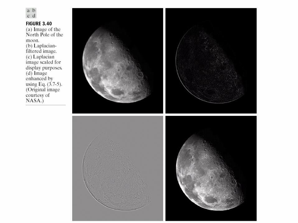
Laplacian

• Digital implementation:

• Two definitions of Laplacian: one is the negative of the other

• Accordingly, to recover background features:

I: if the center of the mask is negativeII: if the center of the mask is positive

€

∇2 f = [ f (x +1,y) + f (x −1,y) + f (x,y +1) + f (x,y −1)] − 4 f (x,y)

€

g(x,y) = {f ( x,y )+∇2 f ( x,y )( II )

f ( x,y )−∇2 f ( x,y )( I )

Simplification

• Filter and recover original part in one step:

€

g(x,y) = f (x,y) −[ f (x +1,y) + f (x −1,y) + f (x,y +1) + f (x,y −1)] + 4 f (x,y)

€

g(x,y) = 5 f (x,y) −[ f (x +1,y) + f (x −1,y) + f (x,y +1) + f (x,y −1)]

Image Enhancement in theSpatial Domain

Image Enhancement in theSpatial Domain

Image Enhancement in theSpatial Domain

Image Enhancement in theSpatial Domain

High-boost Filtering

• Unsharp masking: • Highpass filtered image =

Original – lowpass filtered image.

• If A is an amplification factor then:

– High-boost = A · original – lowpass (blurred) = (A-1) · original + original –

lowpass = (A-1) · original + highpass

€

fs(x,y) = f (x,y) − f (x,y)

High-boost Filtering

• A=1 : standard highpass result

• A>1 : the high-boost image looks more like the original with a degree of edge enhancement, depending on the value of A.

w=9A-1, A≥1

Image Enhancement in theSpatial Domain

Image Enhancement in theSpatial Domain

1st Derivatives• The most common method of differentiation in

Image Processing is the gradient:

€

∇F =GxGy

⎡

⎣ ⎢

⎤

⎦ ⎥=

∂f

∂x∂f

∂y

⎡

⎣

⎢ ⎢ ⎢

⎤

⎦

⎥ ⎥ ⎥

at (x,y)

• The magnitude of this vector is:

€

∇f = mag(∇f ) = [Gx2 +Gy

2]1

2 =∂f

∂x

⎛

⎝ ⎜

⎞

⎠ ⎟2

+∂f

∂y

⎛

⎝ ⎜

⎞

⎠ ⎟

2 ⎡

⎣ ⎢ ⎢

⎤

⎦ ⎥ ⎥

1/ 2

The Gradient• Non-isotropic• Its magnitude (often call the gradient) is

rotation invariant• Computations:

• Roberts uses:

• Approximation (Roberts Cross-Gradient Operators): €

∇f ≈ Gx + Gy

€

Gx = (z9 − z5)

Gy = (z8 − z6)

€

∇f ≈ z9 − z5 + z8 − z6

Derivative Filters

At z5, the magnitude can be approximated as:

€

∇f ≈ [(z5 − z8)2 + (z5 − z6)2]1/ 2

|||| 6585 zzzzf −+−≈∇

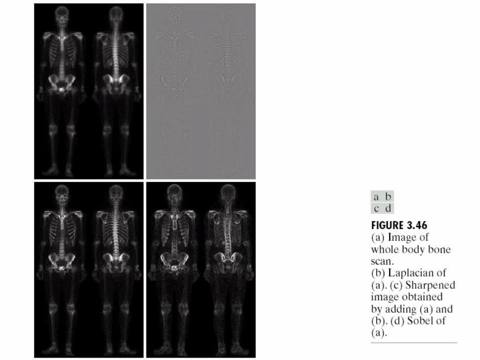
Derivative Filters

• Another approach is:

• One last approach is (Sobel Operators):

2/1286

295 ])()[( zzzzf −+−≈∇

|||| 8695 zzzzf −+−≈∇

€

∇f = (z7 + 2z8 + z9) − (z1 + 2z2 + z3) + (z3 + 2z6 + z9) − (z1 + 2z4 + z7)

Image Enhancement in theSpatial Domain

Image Enhancement in theSpatial Domain