· 2 Journal of Applied Mathematics where Cj 1,...,j m i 1,...,i n ∈ R, i 1,...,i n,j 1,...,j m...

Hindawi Publishing CorporationJournal of Applied MathematicsVolume 2012, Article ID 201340, 24 pagesdoi:10.1155/2012/201340

Research ArticleThe Asymptotic Expansion Method viaSymbolic Computation

Juan F. Navarro

Departamento de Matematica Aplicada, Universidad de Alicante, Carretera San Vicente del Raspeig s/n,03690 San Vicente del Raspeig, Alicante, Spain

Correspondence should be addressed to Juan F. Navarro, [email protected]

Received 26 October 2011; Revised 25 March 2012; Accepted 26 March 2012

Academic Editor: B. V. Rathish Kumar

Copyright q 2012 Juan F. Navarro. This is an open access article distributed under the CreativeCommons Attribution License, which permits unrestricted use, distribution, and reproduction inany medium, provided the original work is properly cited.

This paper describes an algorithm for implementing a perturbation method based on anasymptotic expansion of the solution to a second-order differential equation. We also introducea new symbolic computation system which works with the so-called modified quasipolynomials,as well as an implementation of the algorithm on it.

1. Introduction

The origin of symbolic manipulation derives from the sheer magnitude of the work involvedin the building of perturbation theories, which made inevitable that scientific communitybecame interested in the possibility of constructing those theories with the help of computers.

Perturbation theories for differential equations containing a small parameter ε arequite old. The small perturbation theory originated by Sir Isaac Newton has been highlydeveloped by many others, and an extension of this theory to the asymptotic expansion,consisting of a power series expansion in the small parameter, was devised by Poincare (1892)[1]. The main point is that for the most of the differential equations, it is not possible to obtainan exact solution. In cases where equations contain a small parameter, we can consider it asa perturbation parameter to obtain an asymptotic expansion of the solution. In practice, thework involved in the application of this approach to compute the solution to a differentialequation cannot be performed by hand, and algebraic processors seem to be a very usefultool.

As explained in [2], the first symbolic processors were developed toworkwith Poissonseries, that is, multivariate Fourier series whose coefficients are multivariate Laurent series,

∑

i1,...,in

∑

j1,...,jm

Cj1,...,jmi1,...,in

xi11 x

i22 · · ·xin

ncossin

(j1φ1 + · · · + jmφm

), (1.1)

2 Journal of Applied Mathematics

where Cj1,...,jmi1,...,in

∈ R, i1, . . . , in, j1, . . . , jm ∈ Z, and x1, . . . , xn and φ1, . . . , φm are calledpolynomial and angular variables, respectively. These processors were applied to problemsin nonlinear mechanics or nonlinear differential equations problems, in the field of CelestialMechanics.

One of the first applications of these processors was concerned with the theory ofthe Moon. Delaunay invented his perturbation method to treat it and spent 20 years doingalgebraic manipulations by hand to apply it to the problem. Deprit et al. [3, 4] prolongatedthe solution of Delaunay’s work with the help of a special purpose symbolic processor, andHenrard [5] pushed it to order 25. This solution was improved by iteration by Chapront-Touze [6], and planetary perturbations were also introduced by Chapront-Touze [7]. Atpresent, the most complete solution, ELP (Ephemeride Lunaire Parisien) contains more than50000 periodic terms.

But the motion of the Moon is not the only application of algebraic processors. Thereare many problems where the facilities provided by Poisson series processors can lead ratherquickly to very accurate results. As examples, we would like to mention planetary theories,the theory of the rotation of the Earth (e.g., [8]), and artificial satellite theories (AST). Abadet al. [9] have analysed the convenience of developing specific computer algebra systemsin order to deal with AST. As it is explained in detail in their work, the series involved inthe computation of the solution through the application of a Lie transformation have a totalamount of almost 2000000 terms.

Nowadays, many general purpose computer algebra packages—as, for example,Maple, Mathematica, and Matlab—contain tools for the calculation of the solution ofcertain classes of ODEs. All these packages have the advantage of being very general, sothey can deal with a lot of problems of different nature. However, if one is interested inhigher order solutions, the most common perturbation methods tend to produce expressionscontaining thousands of terms, and their treatment with those general processors becomesinefficient.

To achieve better accuracies in the applications of analytical theories, high orders ofthe approximate solution must be computed, making a continuous maintenance and revisionof the existing symbolic manipulation systems necessary, as well as the development of newpackages adapted to the peculiarities of the problem to be treated.

In order to contribute to the solution of this problem, we have developed asymbolic computation package (called MQSP) based on the object-oriented philosophy whichmanipulates objects of the form

∑ν≥0

τσ11 × · · · × τ

σQ

Q tnνeανt(λν cos(ωνt) + μν sin(ωνt)

), (1.2)

where nν ∈ N, αν, ων, λν, μν ∈ R, σν ∈ Z, and τ1, . . . , τQ are real constants withunknown value. We will refer to those elements as modified quasipolynomials [10].The kernel of this symbolic processor has been developed in C++. The operationson series implemented in the manipulator are the usual operations of the Algebraof quasipolynomials: addition, subtraction, multiplication, multiplication by a scalar,differentiation with respect to t, and substitution of a quasipolynomial into an undeterminedcoefficient.

Journal of Applied Mathematics 3

We have also constructed a set of subroutines to deal with the solution to the perturbeddifferential equation

x + a1x + a0x = u(t) + εf(x, x), x(t0) = x0, x(t0) = x0, (1.3)

where a0, a1, t0, x0, x0 ∈ R, u(t) is given by (1.2), and

f(x, x) =M∑

κ=0

∑

0≤ν≤κfν,κ−ν xν xκ−ν, fν,κ−ν ∈ R. (1.4)

In a previous contribution, the author employed the kernel of this processor tocompute periodic solutions in equations of type (1.3) via the Poincare-Lindstedt method[11, 12]. If the unperturbed equation (ε = 0) has periodic solutions and ε is a measure ofthe size of the perturbing terms, then the trajectories for the full system will remain prettyclose to those of the nonperturbed system, for any finite period of time t0 < t < t0 + α (α > 0)with an error not larger thanO(α). In general, even a small perturbation is enough to destroyperiodicity, that is, nonlinearity will end with most of the periodic orbits of the unperturbedsystem, but some of them may persist. To calculate those periodic orbits, the solution and themodified frequency are expanded with respect to the small parameter, allowing to kill secularterms which appear in the recursive scheme.

The aim of this paper is to construct an algorithm to implement the asymptoticexpansion method [13]. This new implementation is general and does not depend on thefunction f(x, x) as given in (1.4), that is, the user does not need to programme the algorithmdescribed in this paper, and only has to introduce the adequate parameters when callingthe corresponding routine of the package. The code of this specific symbolic system is notavailable on internet but it can be provided by contacting its author.

2. Data Structure

The algorithms that can be implemented to perform the basic manipulation on a series andtheir efficiency depend on the way a series is coded. An overcoded structure that makes gooduse of memory generally requires complex algorithms, which increase the computationalcost in terms of time. On the other hand, an undercoded computational representation ofthe terms generates simple algorithms, because the location of all the coefficients can beobtained directly. However, this scheme presents the inconvenience of being very wastefulin the memory resources required for the storage of the series [2].

In this section, we follow San-Juan and Abad [14] to introduce the representation of amathematical object in a computer. To that purpose, let us introduce the concepts of normaland canonical functions. Let E be a set of symbolic objects, and let ∼ be an equivalence relationin E, defined as follows: a ∼ b if a = b, with a, b ∈ E. Here, the operator = is considered as theequality on the mathematical object level. Moreover, a ≡ b if a and b are identical as symbolicobjects. A function f : E → E is said to be normal in (E,∼) if f(a) ∼ a for all a ∈ E, and fis said to be canonical in (E,∼) if it is normal and a ∼ b ⇒ f(a) = f(b) for all a, b ∈ E. Thus,


a canonical function provides identical objects when objects are equivalent, that is, when theyrepresent the same mathematical object.

For the sake of simplicity, let us focus our attention on the set of quasipolynomials inthe independent variable Q[t]. A quasipolynomial is a map u : R → R, defined by

u(t) =∑

ν≥0tnνeανt

(λν cos(ωνt) + μν sin(ωνt)

), (2.1)

where nν ∈ N, αν, ων, λν, and μν ∈ R. Let us now consider the set of quasipolynomials in theindependent variable t, Q[t].

2.1. QuasiPolynomials as Symbolic Objects

We look for a canonical representation for each equivalence class defined in Q[t]. For thatpurpose, the following operations must be performed over each quasipolynomial.

(1) Let us consider a quasipolynomial u(t) =∑

ν≥0 tnνeανt(λν cos(ωνt) + μν sin(ωνt)). If

ων < 0, the following rules must be applied:

sin(−ωνt) = − sin(ωνt), cos(−ωνt) = cos(ωνt). (2.2)

(2) The terms of a quasipolynomial will be ordered as follows: let us consider two termof a quasipolynomial: τ1 = tn1eα1t(λ1 cosω1t+μ2 sinω1t) and τ2 = tn2eα2t(λ2 cosω2t+μ2 cosω2t). We say that τ1 < τ2 if (n1 < n2) or (n1 = n2 and α1 < α2) or (n1 = n2,α1 = α2, andω1 < ω2) or (n1 = n2, α1 = α2,ω1 = ω2, and λ1 < λ2) or (n1 = n2, α1 = α2,ω1 = ω2, λ1 < λ2, and μ1 < μ2).

(3) The terms of a quasipolynomial

u(t) =∑

ν≥0tnνeανt

(λν cos(ωνt) + μν sin(ωνt)

)(2.3)

with identical values of nν, αν, and ων must be grouped together.

2.2. QuasiPolynomials as Computational Objects

In this section, we will consider the basic information which characterizes a quasipolynomial,as well as the data structure to store it in the computer. This must be done preserving thecanonical representation we have chosen.

Each quasipolynomial is collected in a sorted dynamical list: a sorted list is one inwhich the order of the items is defined by some collating sequence. The codification ofeach term of the list contained in a quasipolynomial is statical, and given by the followingelements.

(1) λ, μ ∈ R are the coefficients of the term.

(2) n ∈ N is the degree of the monomial t.


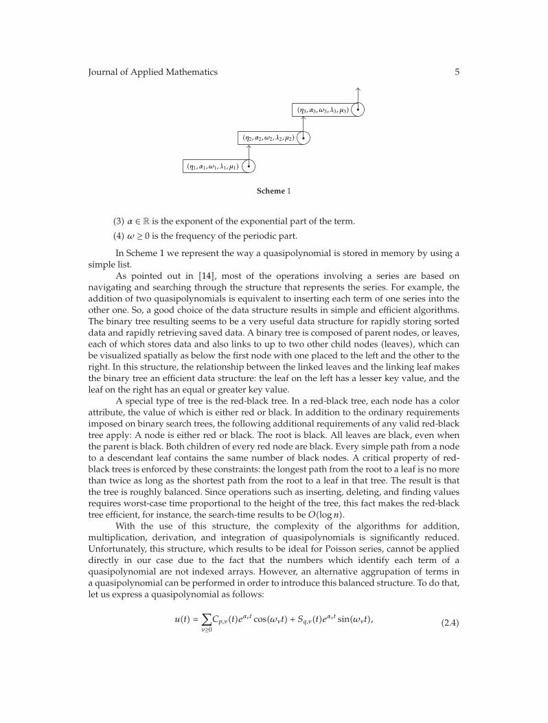
(η1, α1, ω1, λ1, μ1)

(η2, α2, ω2, λ2, μ2)

(η3, α3, ω3, λ3, μ3)

Scheme 1

(3) α ∈ R is the exponent of the exponential part of the term.

(4) ω ≥ 0 is the frequency of the periodic part.

In Scheme 1 we represent the way a quasipolynomial is stored in memory by using asimple list.

As pointed out in [14], most of the operations involving a series are based onnavigating and searching through the structure that represents the series. For example, theaddition of two quasipolynomials is equivalent to inserting each term of one series into theother one. So, a good choice of the data structure results in simple and efficient algorithms.The binary tree resulting seems to be a very useful data structure for rapidly storing sorteddata and rapidly retrieving saved data. A binary tree is composed of parent nodes, or leaves,each of which stores data and also links to up to two other child nodes (leaves), which canbe visualized spatially as below the first node with one placed to the left and the other to theright. In this structure, the relationship between the linked leaves and the linking leaf makesthe binary tree an efficient data structure: the leaf on the left has a lesser key value, and theleaf on the right has an equal or greater key value.

A special type of tree is the red-black tree. In a red-black tree, each node has a colorattribute, the value of which is either red or black. In addition to the ordinary requirementsimposed on binary search trees, the following additional requirements of any valid red-blacktree apply: A node is either red or black. The root is black. All leaves are black, even whenthe parent is black. Both children of every red node are black. Every simple path from a nodeto a descendant leaf contains the same number of black nodes. A critical property of red-black trees is enforced by these constraints: the longest path from the root to a leaf is no morethan twice as long as the shortest path from the root to a leaf in that tree. The result is thatthe tree is roughly balanced. Since operations such as inserting, deleting, and finding valuesrequires worst-case time proportional to the height of the tree, this fact makes the red-blacktree efficient, for instance, the search-time results to be O(logn).

With the use of this structure, the complexity of the algorithms for addition,multiplication, derivation, and integration of quasipolynomials is significantly reduced.Unfortunately, this structure, which results to be ideal for Poisson series, cannot be applieddirectly in our case due to the fact that the numbers which identify each term of aquasipolynomial are not indexed arrays. However, an alternative aggrupation of terms ina quasipolynomial can be performed in order to introduce this balanced structure. To do that,let us express a quasipolynomial as follows:

u(t) =∑

ν≥0Cp,ν(t)eανt cos(ωνt) + Sq,ν(t)eανt sin(ωνt), (2.4)


SIN

SIN

COS

COS

...

...

...

...

...

...

...

...

σ2,i + 1, μ2,i + 1

σ2,i , μ2,i

σ2,i − 1, μ2,i − 1

ν2,i, λ2,i

ν2,i + 1, λ2,i + 1

ν2,i − 1, λ2,i − 1

σ1,i , μ1,i

σ1,i + 1, μ1,i + 1

σ1,i − 1, μ1,i − 1

ν1,i, λ1,i

ν1,i + 1, λ1,i + 1

ν1,i − 1, λ1,i − 1

(α2, ω2)

(α1, ω1)

Scheme 2

whereCp,ν(t) and Sq,ν(t) are polynomials in the variable twith constant coefficients, of degreep and q respectively, being p, q ∈ N:

Cp,ν(t) = λ0 + λ1t + λ2t2 + · · · + λpt

p,

Sq,ν(t) = μ0 + μ1t + μ2t2 + · · · + μqt

q,(2.5)

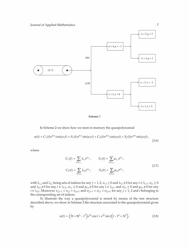
with λ0, λ1, . . . , λp, μ0, μ1, . . . , μq ∈ R. If we aggrupate terms of a quasipolynomial in such amanner, we can use a tree structure to store it, saving only significant terms. In Scheme 2 weshow the tree structure in which the quasipolynomial is stored.


SIN

COS

σ = 4, μ = −1

σ = 7, μ = 3

σ = 1, μ = 1

ν = 7, λ = −1

ν = 1, λ = 3

(2, 1)

ν = 3, λ = 8

Scheme 3

In Scheme 2 we show how we store in memory the quasipolynomial

u(t) = C1(t)eα1t cos(ω1t) + S1(t)eα1t sin(ω1t) + C2(t)eα2t cos(ω2t) + S2(t)eα2t sin(ω2t),(2.6)

where

C1(t) =∑

i∈IC,1

λ1,itν1,i , S1(t) =

∑

i∈IS,1

μ1, itσ1,i ,

C2(t) =∑

i∈IC,2

λ2,itν2,i , S2(t) =

∑

i∈IS,2

μ2,itσ2,i ,

(2.7)

with IC,j and IS,j being sets of indices for any j = 1, 2, ν1,i ≥ 0 and λ1,i /= 0 for any i ∈ IC,1, ν2,i ≥ 0and λ2,i /= 0 for any i ∈ IC,2, σ1,i ≥ 0 and μ1,i /= 0 for any i ∈ IS,1, and σ2,i ≥ 0 and μ2,i /= 0 for anyi ∈ IS,2. Moreover, νj,i−1 < νj,i < νj,i+1 and σj,i−1 < σj,i < σj,i+1 for any j = 1, 2 and i belonging tothe corresponding set of indices.

To illustrate the way a quasipolynomial is stored by means of the tree structuredescribed above, we show in Scheme 3 the structure associated to the quasipolynomial givenby

u(t) =(3t + 8t3 − t7

)e2t cos t + e2t sin t

(t − t4 + 3t7

). (2.8)


Table 1: Some examples of representation of terms.

Term λ μ σ1 σ2 σ3 σ4 n α ω

3τ21 τ4 cos(5t) 3 0 2 0 0 1 0 0 5−τ1τ2τ23 t7e−t sin(3t) 0 −1 1 1 2 0 7 −1 32τ2τ23 te

2t cos(3t) 2 0 0 1 2 0 1 2 3

2.3. Modified QuasiPolynomials as Computational Objects

In our symbolic system, we represent a modified quasipolynomial by an ordered anddynamical list of terms, keeping in memory only significant terms. The codification of a termis statical, and given by the following elements.

(1) λ, μ ∈ R are the coefficients of the term (for cos and sin, resp.).

(2) (σ1, . . . , σQ) ∈ ZQ. For each 0 ≤ ν ≤ Q, σν represents the exponent of the

undetermined coefficient τν.

(3) n ∈ N is the degree of the monomial t.

(4) α ∈ R is the exponent of the exponential part of the term.

(5) ω ≥ 0 is the frequency of the periodic part.

We have included the two following additional vectors, which are common to all theterms of a modified quasipolynomial:

(1) (m1, . . . , mQ) ∈ {0, 1}Q. For each 0 ≤ ν ≤ Q, mν = 0 indicates that τν is a coefficientwith unknown value, while mν = 1 implies that τν has a real value assigned,

(2) τ = (τ1, . . . , τQ) ∈ RQ. If the coefficient τν has a real value assigned, its content is

given by τν, for each 0 ≤ ν ≤ Q.

It is also absolutely essential to store the number of undetermined coefficients that arecurrently in use, to generate correctly new undetermined constants if needed. In Table 1 weillustrate the way a term is coded with a few examples, where it has been assumed thatQ = 4.

3. Design of the Symbolic System in C++

As pointed out in [15], object-oriented programming using C++ provides many advantagesin the design of computer algebra systems, as this programming technique combines boththe data and the functions that operate on that data into a single unit (called class). The mainreasons given by Hardy et al. to use C++ to implement a symbolic system are as follows.

(1) C++ allows the introduction of abstract data types. Thus, we can define a modifiedquasipolynomial as an abstract data type.

(2) The language C++ supports encapsulation, inheritance, polymorphism, andoperator overloading. Consequently, we can overload the operators +, −, and ∗for modified quasipolynomials, as well as ∗ and/for multiplication and divisionof modified quasipolynomials by real numbers.

Some symbolic computation systems have been constructed in C++. MuPAD is acomputer algebra system developed by the MuPAD research group at the University of


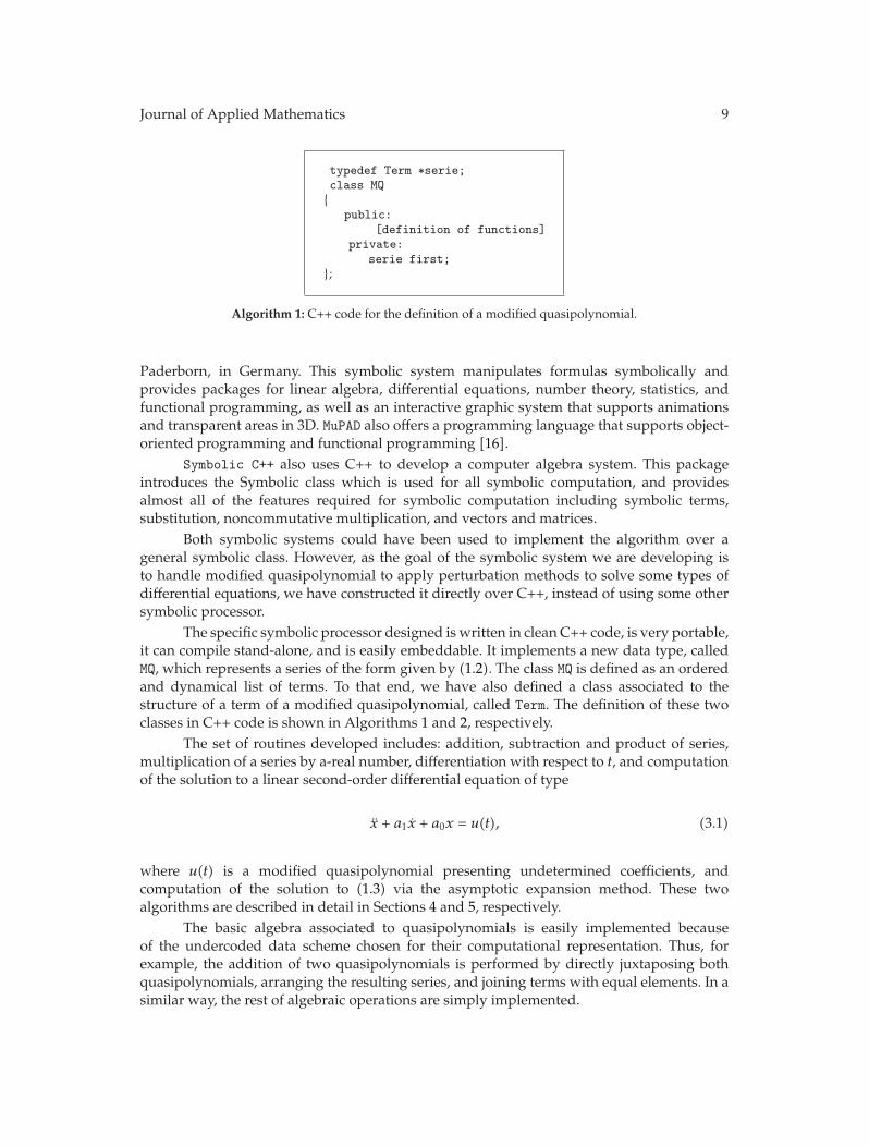
typedef Term ∗serie;class MQ

{public:

[definition of functions]private:

serie first;};

Algorithm 1: C++ code for the definition of a modified quasipolynomial.

Paderborn, in Germany. This symbolic system manipulates formulas symbolically andprovides packages for linear algebra, differential equations, number theory, statistics, andfunctional programming, as well as an interactive graphic system that supports animationsand transparent areas in 3D. MuPAD also offers a programming language that supports object-oriented programming and functional programming [16].

Symbolic C++ also uses C++ to develop a computer algebra system. This packageintroduces the Symbolic class which is used for all symbolic computation, and providesalmost all of the features required for symbolic computation including symbolic terms,substitution, noncommutative multiplication, and vectors and matrices.

Both symbolic systems could have been used to implement the algorithm over ageneral symbolic class. However, as the goal of the symbolic system we are developing isto handle modified quasipolynomial to apply perturbation methods to solve some types ofdifferential equations, we have constructed it directly over C++, instead of using some othersymbolic processor.

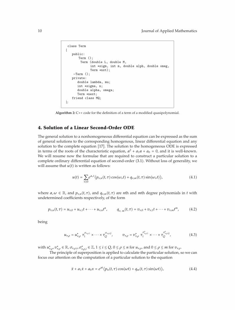
The specific symbolic processor designed is written in clean C++ code, is very portable,it can compile stand-alone, and is easily embeddable. It implements a new data type, calledMQ, which represents a series of the form given by (1.2). The class MQ is defined as an orderedand dynamical list of terms. To that end, we have also defined a class associated to thestructure of a term of a modified quasipolynomial, called Term. The definition of these twoclasses in C++ code is shown in Algorithms 1 and 2, respectively.

The set of routines developed includes: addition, subtraction and product of series,multiplication of a series by a-real number, differentiation with respect to t, and computationof the solution to a linear second-order differential equation of type

x + a1x + a0x = u(t), (3.1)

where u(t) is a modified quasipolynomial presenting undetermined coefficients, andcomputation of the solution to (1.3) via the asymptotic expansion method. These twoalgorithms are described in detail in Sections 4 and 5, respectively.

The basic algebra associated to quasipolynomials is easily implemented becauseof the undercoded data scheme chosen for their computational representation. Thus, forexample, the addition of two quasipolynomials is performed by directly juxtaposing bothquasipolynomials, arranging the resulting series, and joining terms with equal elements. In asimilar way, the rest of algebraic operations are simply implemented.


class Term{

public:Term ();Term (double L, double M,

int ∗sigm, int m, double alph, double omeg,Term ∗nxt);

∼Term ();private:

double lambda, mu;int ∗sigma, n;double alpha, omega;Term ∗next;

friend class MQ;};

Algorithm 2: C++ code for the definition of a term of a modified quasipolynomial.

4. Solution of a Linear Second-Order ODE

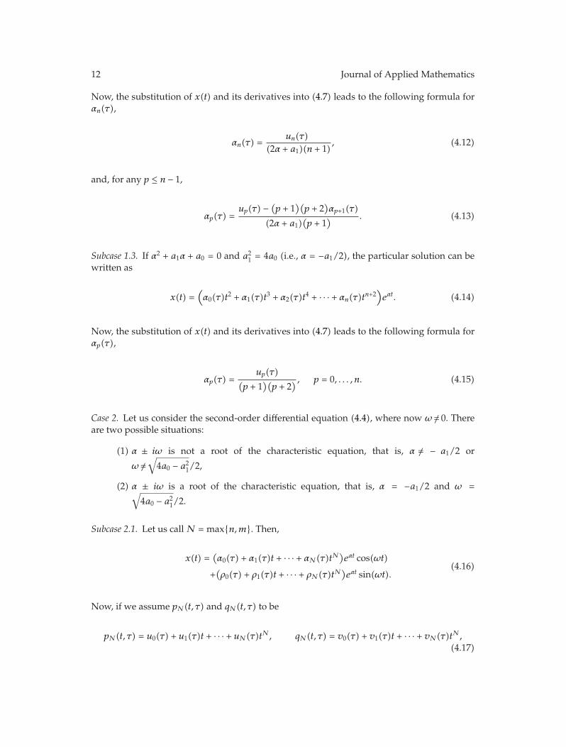
The general solution to a nonhomogeneous differential equation can be expressed as the sumof general solutions to the corresponding homogenous, linear differential equation and anysolution to the complete equation [17]. The solution to the homogeneous ODE is expressedin terms of the roots of the characteristic equation, α2 + a1α + a0 = 0, and it is well-known.We will resume now the formulae that are required to construct a particular solution to acomplete ordinary differential equation of second-order (3.1). Without loss of generality, wewill assume that u(t) is written as follows:

u(t) =∑

ν≥0eανt

(pν,n(t, τ) cos(ωνt) + qν,m(t, τ) sin(ωνt)

), (4.1)

where α,ω ∈ R, and pν,n(t, τ), and qν,m(t, τ) are nth and mth degree polynomials in t withundetermined coefficients respectively, of the form

pν,n(t, τ) = uν,0 + uν,1t + · · · + uν,ntn, qν, m(t, τ) = vν,0 + vν,1t + · · · + vν,mt

m, (4.2)

being

uν,ρ = u∗ν,ρ τ

σν,ρ,1

1 × · · · × τσν,ρ,Q

Q , vν,ρ = v∗ν,ρ τ

σ∗ν,ρ,1

1 × · · · × τσ∗ν,ρ,Q

Q , (4.3)

with u∗ν,ρ, v

∗ν,ρ ∈ R, σν,ρ,i, σ

∗ν,ρ,i ∈ Z, 1 ≤ i ≤ Q, 0 ≤ ρ ≤ n for uν,ρ, and 0 ≤ ρ ≤ m for vν,ρ.

The principle of superposition is applied to calculate the particular solution, so we canfocus our attention on the computation of a particular solution to the equation

x + a1x + a0x = eαt(pn(t, τ) cos(ωt) + qm(t, τ) sin(ωt)

), (4.4)


where

pn(t, τ) = u0 + u1t + · · · + untn, qm(t, τ) = v0 + v1t + · · · + vmt

m, (4.5)

being

uρ = u∗ρ τ

σρ,1

1 × · · · × τσρ,Q

Q , vρ = v∗ρ τ

σ∗ρ,1

1 × · · · × τσ∗ρ,Q

Q , (4.6)

with u∗ρ, v

∗ρ ∈ R, σρ,i, σ

∗ρ,i ∈ Z, 1 ≤ i ≤ Q, 0 ≤ ρ ≤ n for uρ, and 0 ≤ ρ ≤ m for vρ.

At this point, we will distinguish two cases depending on if ω = 0 or ω/= 0.

Case 1. Let us consider the second-order ODE (4.4), with ω = 0. Then, the equation is writtenas

x + a1x + a0x = pn(t, τ)eαt, (4.7)

where pn(t, τ) is given by (4.5).

Subcase 1.1. If α2 + a1α + a0 /= 0, the particular solution to the complete differential equation isexpressed as

x(t) =(α0(τ) + α1(τ)t + α2(τ)t2 + · · · + αn(τ)tn

)eαt. (4.8)

Thus, substituting x(t) and its derivatives in (4.7), we get that

αn(τ) =un(τ)

α2 + a1α + a0, αn−1(τ) =

un−1(τ) − (a1 + 2α)nαn(τ)α2 + a1α + a0

, (4.9)

and, for any p < n − 1,

αp(τ) =up(τ) − (a1 + 2α)

(p + 1

)αp+1(τ) −

(p + 1

)(p + 2

)αp+2(τ)

α2 + a1α + a0. (4.10)

Subcase 1.2. If α2 + a1α + a0 = 0 and a21 /= 4a0 (i.e., α/= − a1/2), the particular solution can be

written as

x(t) =(α0(τ)t + α1(τ)t2 + α2(τ)t3 + · · · + αn(τ)tn+1

)eαt. (4.11)


Now, the substitution of x(t) and its derivatives into (4.7) leads to the following formula forαn(τ),

αn(τ) =un(τ)

(2α + a1)(n + 1), (4.12)

and, for any p ≤ n − 1,

αp(τ) =up(τ) −

(p + 1

)(p + 2

)αp+1(τ)

(2α + a1)(p + 1

) . (4.13)

Subcase 1.3. If α2 + a1α + a0 = 0 and a21 = 4a0 (i.e., α = −a1/2), the particular solution can be

written as

x(t) =(α0(τ)t2 + α1(τ)t3 + α2(τ)t4 + · · · + αn(τ)tn+2

)eαt. (4.14)

Now, the substitution of x(t) and its derivatives into (4.7) leads to the following formula forαp(τ),

αp(τ) =up(τ)(

p + 1)(p + 2

) , p = 0, . . . , n. (4.15)

Case 2. Let us consider the second-order differential equation (4.4), where now ω/= 0. Thereare two possible situations:

(1) α ± iω is not a root of the characteristic equation, that is, α /= − a1/2 or

ω/=√4a0 − a2

1/2,

(2) α ± iω is a root of the characteristic equation, that is, α = −a1/2 and ω =√4a0 − a2

1/2.

Subcase 2.1. Let us call N = max{n,m}. Then,

x(t) =(α0(τ) + α1(τ)t + · · · + αN(τ)tN

)eαt cos(ωt)

+(ρ0(τ) + ρ1(τ)t + · · · + ρN(τ)tN

)eαt sin(ωt).

(4.16)

Now, if we assume pN(t, τ) and qN(t, τ) to be

pN(t, τ) = u0(τ) + u1(τ)t + · · · + uN(τ)tN, qN(t, τ) = v0(τ) + v1(τ)t + · · · + vN(τ)tN,(4.17)


and substitute x(t) and its derivatives into (4.4), we get that

αN(τ) =1Δ

∣∣∣∣∣uN(τ) ω(a1 + 2α)

vN(τ) a0 + a1α + α2 −ω2

∣∣∣∣∣,

ρN(τ) =1Δ

∣∣∣∣∣a0 + a1α + α2 −ω2 uN(τ)

−ω(a1 + 2α) vN(τ)

∣∣∣∣∣,

(4.18)

where Δ = (a0 + a1α + α2 −ω2)2 +ω2(a1 + 2α)2. Note that Δ/= 0, because a0 + a1α + α2 −ω2 /= 0or ω(2α + a1)/= 0. Now, we can compute αN−1(τ) and ρN−1(τ) by solving the system

uN−1(τ) −N(a1 + 2α) αN(τ) − 2NωρN(τ)

=(a0 + a1α + α2 −ω2

)αN−1(τ) + (a1ω + 2αω)ρN−1(τ),

vN−1(τ) −N(a1 + 2α)ρN(τ) + 2NωαN(τ)

= −ω(a1 + 2α)αN−1(τ) +(a0 + a1α + α2 −ω2

)ρN−1(τ).

(4.19)

As before, this system can be solved by applying the Cramer’s rule. Finally, for any p < N−1,we have to solve the system in αp(τ) and ρp(τ), as follows:

up(τ) −(p + 2

)(p + 1

)αp+2(τ) −

(p + 1

)(a1 + 2α) αp+1(τ) − 2

(p + 1

)ωρp+1(τ)

=(a0 + a1α + α2 −ω2

)αp(τ) +ω(a1 + 2α)ρp(τ),

vp(τ) −(p + 2

)(p + 1

)ρp+2(τ) −

(p + 1

)(a1 + 2α) ρp+1(τ) + 2

(p + 1

)ωαp+1(τ)

= −ω(a1 + 2α)αp(τ) +(a0 + a1α + α2 −ω2

)ρp(τ).

(4.20)

Subcase 2.2. Now we consider the case where α = −a1/2 and ω =√4a0 − a2

1/2. This impliesthat a1 + 2α = 0 and α2 −ω2 +a1α+a0 = 0. In this case, the particular solution adopts the form

x(t) =(α0(τ)t + α1(τ)t2 + α2(τ)t3 + · · · + αN(τ)tN+1

)eαt cos(ωt)

+(ρ0(τ)t + ρ1(τ)t2 + ρ2(τ)t3 + · · · + ρN(τ)tN+1

)eαt sin(ωt),

(4.21)


and substituting x(t), x(t), and x(t) into (4.4), we obtain

ρN(τ) =uN(τ)

2(N + 1)ω, αN(τ) = − vN(τ)

2(N + 1)ω,

ρp(τ) =up(τ) −

(p + 1

)(p + 2

)αp+1

2(p + 1

)ω

, αp(τ) =vp(τ) −

(p + 1

)(p + 2

)ρp+1

−2(p + 1)ω

,

(4.22)

for any p < N.From (4.8)–(4.22), it is a straightforward task; the derivation of an algorithm for the

computation of the solution to (4.4).

5. Computation of the Solution to the Perturbed Problem

The symbolic package is thought to compute the solution to (1.3). The standard approach[13] is to try a power series solution of the form

x(t, ε) = x0(t) + x1(t) ε + x2(t) ε2 + · · · . (5.1)

This series is inserted into the governing equation and initial conditions, and coefficientsof same powers of ε are then grouped to obtain a collection of equations for the coefficientfunctions xi(t), which are then solved in a sequential manner. The resulting series need notconverge for any value of ε; nevertheless, the solution x(t, ε) can be useful in approximatingthe function when ε is small.

Considering the zero-order term in ε yields

x0 + a1x0 + a0x0 = u(t), x(t0) = x0, x(t0) = x0, (5.2)

the so-called nonperturbed problem. The symbolic manipulation system calculates thesolution to a differential equation of the form (5.2), and arranges it as a quasipolynomial,as it has been described in detail in the previous section.

The coefficient xq(t) of the solution to the order q ≥ 1 is computed by solving theequation

xq + a1xq + a0xq =M∑

κ=0

∑

0≤ν≤κfν,κ−ν

(xν xκ−ν)

q−1, xq(t0) = 0, xq(t0) = 0, (5.3)

where the notation (xνxκ−ν)q refers to the qth order term of the series xνxκ−ν.


At each order of the solution, the series (xν)q, (xν)q, and (xνxκ−ν)q must be computed

once the order q has been solved, for each q ≥ 0, following the formulae

(xν)q =∑

0≤p≤q

(xν−1

)

p(x)q−p,

(xν)q =∑

0≤p≤q

(xν−1

)

p(x)q−p,

(xνxκ−ν)

q =∑

0≤p≤q(xν)p

(xκ−ν)

q−p.

(5.4)

According to this, the algorithm to apply the asymptotic expansion method to solvethe initial value problem given by (1.3), consists of the following steps.

(1) Define a three-dimensional array of quasipolynomials X(ρ1, ρ2, q), where ρ1, ρ2, q ∈N, 0 ≤ ρ1, ρ2 ≤ M, and 0 ≤ q ≤ Q, Q being the order of the asymptotic expansion.

(2) Define an array of quasipolynomials x(ρ), where 0 ≤ ρ ≤ Q.

(3) Initialize X(0, 0, 0) = 1, and proceed as follows:

(3.1) Compute X(1, 0, 0) as the solution to (5.2).(3.2) Compute X(0, 1, 0) = d/dt(X(1, 0, 0)).(3.3) Calculate, for each ρ such that 2 ≤ ρ ≤ M,

X(ρ, 0, 0

)= X(1, 0, 0) ×X

(ρ − 1, 0, 0

),

X(0, ρ, 0

)= X(0, 1, 0) ×X

(0, ρ − 1, 0

).

(5.5)

(3.4) For each ρ1, ρ2 such that 1 ≤ ρ1, ρ2 ≤ M, determine the quasipolynomial

X(ρ1, ρ2, 0

)= X

(ρ1, 0, 0

) ×X(0, ρ2, 0

). (5.6)

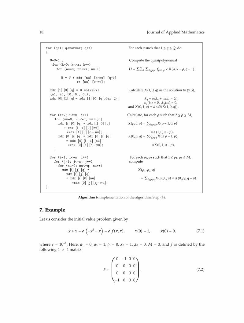
(4) For each q such that 1 ≤ q ≤ Q, do the following.

(4.1) Compute the quasipolynomial

U =M∑

κ=0

∑

0≤ρ≤κfρ,κ−ρ ×X

(ρ, κ − ρ, q − 1

). (5.7)

(4.2) Calculate X(1, 0, q) as the solution to (5.3),

xq + a1xq + a0xq = U, xq(t0) = 0, xq(t0) = 0. (5.8)

(4.3) Compute X(0, 1, q) = d/dt(X(1, 0, q)).


(4.4) Calculate, for each ρ such that 2 ≤ ρ ≤ M,

X(ρ, 0, q

)=

∑

0≤p≤qX(ρ − 1, 0, p

) ×X(1, 0, q − p

),

X(0, ρ, q

)=

∑

0≤p≤qX(0, ρ − 1, p

) ×X(0, 1, q − p

).

(5.9)

(4.5) For each ρ1, ρ2 such that 1 ≤ ρ1, ρ2 ≤ M, compute

X(ρ1, ρ2, q

)=

∑

0≤p≤qX(ρ1, 0, p

) ×X(0, ρ2, q − p

). (5.10)

(5) For each ρ such that 0 ≤ ρ ≤ Q,

x(ρ)= X

(1, 0, ρ

), x(t) =

∑

0≤ρ≤Qερx

(ρ). (5.11)

The input arguments of the algorithm consist of the order Q of the asymptoticapproximation, the coefficients a1, a0 of the differential equation, the real values t0, x0, andx0 which define the initial conditions of the problem, the quasipolynomial u(t), and theperturbed part of the equation f(x, x). As f can be written as given in (1.4),

f(x, x) =M∑

κ=0

∑

0≤ν≤κfν,κ−ν xν xκ−ν, (5.12)

it can be specified by a real (M + 1) × (M + 1) matrix,

f(x, x) =(1 x · · · xM

)

⎛⎜⎜⎜⎜⎜⎜⎝

f00 f01 · · · f0M

f10 f11 · · · f1M

......

. . ....

fM0 fM1 · · · fMM

⎞⎟⎟⎟⎟⎟⎟⎠

⎛⎜⎜⎜⎜⎜⎜⎝

1

x

...

xM

⎞⎟⎟⎟⎟⎟⎟⎠

. (5.13)

The parameter M is also required as input.The output argument of the algorithm is the array x(ρ) containing the coefficients of

the asymptotic expansion. The asymptotic approximation to the order Q is given by

x(t) =∑

0≤ρ≤Qερx

(ρ). (5.14)


MQ xdx [M + 1] [M + 1] [ORDER + 1]; Define a three-dimensional array of quasipolynomials X(ρ1, ρ2, q), where ρ1, ρ2, q ∈N, 0 ≤ ρ1, ρ2 ≤ M and 0 ≤ q ≤ Q, beingQ the order of the asymptotic expansion.

MQ ∗s; Define an array of quasipolynomials x(ρ),s=new MQ [ORDER + 1]; where 0 ≤ ρ ≤ Q.

int i, j, k, p, q, nu; Definition of auxiliary variables.MQ U;

Algorithm 3: Implementation of the algorithm. Steps (1) and (2).

xdx [0] [0] [0].add Initialize X(0, 0, 0) = 1.(1., 0., 0, 0., 0.);

xdx [1] [0] [0] = u.solvePVI Compute X(1, 0, 0) as the solution to (5.2),(a1, a0, t0, x0, dx0); and X(0, 1, 0) = d/dt(X(1, 0, 0)).xdx [0] [1] [0] = xdx [1] [0] [0].der ();

Algorithm 4: Implementation of the algorithm. Steps (3.1) and (3.2).

for (i = 2; i <= m; i + +){ Calculate, for each ρ such that 2 ≤ ρ ≤ M,xdx [i] [0] [0] =

xdx [1] [0] [0] ∗xdx [i − 1] [0] [0]; X(ρ, 0, 0) = X(1, 0, 0) ×X(ρ − 1, 0, 0),xdx [0] [i] [0] =

xdx [0] [1] [0] ∗xdx [0] [i − 1] [0]; X(0, ρ, 0) = X(0, 1, 0) ×X(0, ρ − 1, 0).

}for (i=1; i<=m; i++) For each ρ1, ρ2 such that 1 ≤ ρ1, ρ2 ≤ M,

for (j=1; j<=m; j++) determine the quasipolynomialxdx [i] [j] [0] =

xdx [i] [0] [0]∗xdx [0] [j] [0]; X(ρ1, ρ2, 0) = X(ρ1, 0, 0) ×X(0, ρ2, 0).

Algorithm 5: Implementation of the algorithm. Steps (3.3) and (3.4).

6. On the Implementation of the Algorithm

In Algorithms 3, 4, 5, 6, and 7 we show the C++ code for the implementation of the algorithmas described in Section 5, omitting error control sentences for the sake of simplicity. The headof the definition of the function that implements the algorithm is shown below.

MQ ∗solveAM (double a1, double a0, double t0, double x0, double dx0, MQu, double ∗∗f, int m, int order)


for (q=1; q<=order; q++) For each q such that 1 ≤ q ≤ Q, do:{

U=U∗0.; Compute the quasipolynomialfor (k=0; k<=m; k++)

for (nu=0; nu<=k; nu++) U =∑M

κ=0∑

0≤ρ≤κ fρ,κ−ρ ×X(ρ, κ − ρ, q − 1).

U = U + xdx [nu] [k-nu] [q-1]∗f [nu] [k-nu];

xdx [1] [0] [q] = U.solvePVI Calculate X(1, 0, q) as the solution to (5.3),(a1, a0, t0, 0., 0.);xdx [0] [1] [q] = xdx [1] [0] [q].der (); xq + a1xq + a0xq = U,

xq(t0) = 0, xq(t0) = 0,and X(0, 1, q) = d/dt(X(1, 0, q)).

for (i=2; i<=m; i++) Calculate, for each ρ such that 2 ≤ ρ ≤ M,for (nu=0; nu<=q; nu++) {xdx [i] [0] [q] = xdx [i] [0] [q] X(ρ, 0, q) =

∑0≤p≤q X(ρ − 1, 0, p)

+ xdx [i − 1] [0] [nu]∗xdx [1] [0] [q − nu]; ×X(1, 0, q − p),

xdx [0] [i] [q] = xdx [0] [i] [q] X(0, ρ, q) =∑

0≤p≤q X(0, ρ − 1, p)+ xdx [0] [i − 1] [nu]∗xdx [0] [1] [q − nu]; ×X(0, 1, q − p).

}

for (i=1; i<=m; i++) For each ρ1, ρ2 such that 1 ≤ ρ1, ρ2 ≤ M,for (j=1; j<=m; j++) compute

for (nu=0; nu<=q; nu++)xdx [i] [j] [q] = X(ρ1, ρ2, q)

xdx [i] [j] [q]+ xdx [i] [0] [nu] =

∑0≤p≤q X(ρ1, 0, p) ×X(0, ρ2, q − p).

∗xdx [0] [j] [q − nu];}

Algorithm 6: Implementation of the algorithm. Step (4).

7. Example

Let us consider the initial value problem given by

x + x = ε(−x3 − x

)= ε f(x, x), x(0) = 1, x(0) = 0, (7.1)

where ε = 10−1. Here, a1 = 0, a0 = 1, t0 = 0, x0 = 1, x0 = 0, M = 3, and f is defined by thefollowing 4 × 4 matrix:

F =

⎛⎜⎜⎜⎜⎜⎝

0 −1 0 0

0 0 0 0

0 0 0 0

−1 0 0 0

⎞⎟⎟⎟⎟⎟⎠

. (7.2)


for (i=0; i<=order; i++){ For each ρ such that 0 ≤ ρ ≤ Q,s [i] = xdx [1] [0] [i];s [i].normalice (); x(ρ) = X(1, 0, ρ), and x(t) =

∑0≤ρ≤Q ερx(ρ).

s [i].order ();s [i].join ();s [i].neglect (PREC);

}

Algorithm 7: Implementation of the algorithm. Step (5).

2

0

1 2 3 4 5 6 7 8 9

−2

Figure 1: Comparison between a fourth order symbolic and a numerical solution.

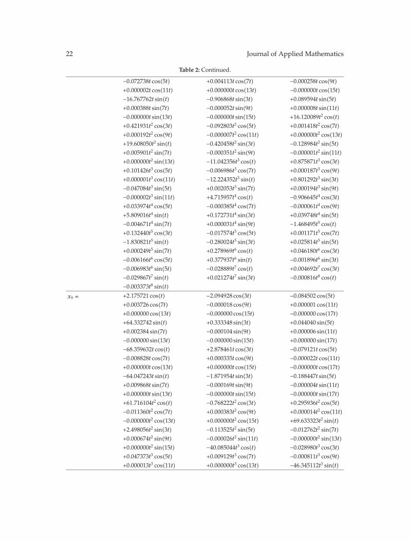
In Table 2 we show the output generated from the symbolic manipulator, just to ordernine for the sake of simplicity, as the number of terms of the asymptotic expansion increasesvery quickly with the order of the expansion.

In Figure 1, we show a comparison of the solution computed through the symbolicmethod (to the fourth-order of the solution) presented in this paper, and the numeric solutionto the problem calculated by a Runge-Kutta fourth-order method with a step of h = 0.001. Letus stress that the difference between both solutions at any time is smaller than 10−7. Thenumerical solution has been calculated with the only purpose of validating the symbolicsolution, as it is not the goal of this paper to develop a numerical tool.

In Table 3, we compare the CPU time of the algorithm implemented with MQSP andMaple running on an iMac 2.8GHz Intel Core 2 Duo. For the test problem described by (7.1),we have calculated the solution up to order 14. In Table 3, we show the CPU time for thedifferent orders of the solution from x0(t) (nonperturbed problem) to x14(t). The computationtime of x4(t) with the use of the dsolve command of Maple in the implementation of thealgorithm is larger than 100 000 seconds. This is due to the fact that dsolve is a general solverwhich handles different types of ordinary differential equations. We have also computedthe symbolic solution taking into account the linearity of (7.1) and implementing a routinefollowing the algorithm detailed in Section 4. These CPU times are given in the fourth columnof Table 3. For orders of the solution larger than 11, Maple does not give any response. We cansee that the difference between MQSP and Maple in terms of CPU time is significant.


Table 2: Some coefficients of the asymptotic expansion of the solution to (7.1).

x0 = +1.000000 cos(t)

x1 = −0.031250 cos(t) +0.031250 cos(3t) +0.500000 sin(t)−0.500000t cos(t) −0.375000t sin(t)

x2 = +0.022461 cos(t) −0.023438 cos(3t) +0.000977 cos(5t)+0.226563 sin(t) +0.070313 sin(3t) −0.390625t cos(t)−0.046875t cos(3t) −0.031250t sin(t) −0.035156t sin(3t)+0.054688t2 cos(t) +0.375000t2 sin(t)

x3 = +0.047760 cos(t) −0.046326 cos(3t) −0.001465 cos(5t)+0.000031 cos(7t) +0.122640 sin(t) −0.005859 sin(3t)+0.003988 sin(5t) −0.201660t cos(t) +0.079102t cos(3t)−0.002441t cos(5t) −0.133057t sin(t) −0.059692t sin(3t)−0.001831t sin(5t) +0.103760t2 cos(t) +0.015381t2 cos(3t)+0.140625t2 sin(t) +0.070313t2 sin(3t) +0.084635t3 cos(t)−0.194336t3 sin(t)

x4 = +0.031557 cos(t) −0.025802 cos(3t) −0.005688 cos(5t)−0.000069 cos(7t) +0.000001 cos(9t) +0.314784 sin(t)+0.001236 sin(3t) −0.003563 sin(5t) +0.000181 sin(7t)−0.329605t cos(t) +0.018219t cos(3t) +0.009552t cos(5t)−0.000107t cos(7t) −0.441519t sin(t) +0.023666t sin(3t)−0.006212t sin(5t) −0.000080t sin(7t) +0.340805t2 cos(t)−0.113068t2 cos(3t) +0.001335t2 cos(5t) +0.323486t2 sin(t)−0.007141t2 sin(3t) +0.005493t2 sin(5t) −0.113566t3 cos(t)+0.031860t3 cos(3t) −0.168498t3 sin(t) −0.064362t3 sin(3t)−0.081533t4 cos(t) +0.060547t4 sin(t)

x5 = +0.101090 cos(t) −0.103018 cos(3t) +0.002327 cos(5t)−0.000396 cos(7t) −0.000003 cos(9t) +0.000000 cos(11t)+0.567049 sin(t) +0.011443 sin(3t) −0.003304 sin(5t)−0.000300 sin(7t) +0.000007 sin(9t) −0.630124t cos(t)+0.042347t cos(3t) +0.004305t cos(5t) +0.000649t cos(7t)−0.000004t cos(9t) −0.861960t sin(t) −0.136819t sin(3t)+0.014968t sin(5t) −0.000407t sin(7t) −0.000003t sin(9t)+0.769419t2 cos(t) +0.056821t2 cos(3t) −0.019625t2 cos(5t)+0.000082t2 cos(7t) +0.653250t2 sin(t) −0.009047t2 sin(3t)−0.002311t2 sin(5t) +0.000320t2 sin(7t) −0.271820t3 cos(t)+0.077614t3 cos(3t) +0.003465t3 cos(5t) −0.512211t3 sin(t)+0.066607t3 sin(3t) −0.007243t3 sin(5t) +0.084625t4 cos(t)−0.054769t4 cos(3t) +0.110530t4 sin(t) +0.027557t4 sin(3t)+0.046019t5 cos(t) −0.005018t5 sin(t)

x6 = +0.041699 cos(t) −0.035635 cos(3t) −0.006540 cos(5t)+0.000498 cos(7t) −0.000022 cos(9t) −0.000000 cos(11t)+0.000000 cos(13t) +1.753506 sin(t) −0.124680 sin(3t)+0.000293 sin(5t) −0.000409 sin(7t) −0.000018 sin(9t)+0.000000 sin(11t) −1.732879t cos(t) +0.361830t cos(3t)−0.007317t cos(5t) +0.000416t cos(7t) +0.000035t cos(9t)


Table 2: Continued.

−0.000000t cos(11t) −1.950362t sin(t) +0.090323t sin(3t)

−0.009679t sin(5t) +0.001762t sin(7t) −0.000022t sin(9t)−0.000000t sin(11t) +1.753296t2 cos(t) −0.260570t2 cos(3t)+0.014763t2 cos(5t) −0.001785t2 cos(7t) +0.000004t2 cos(9t)

+1.911049t2 sin(t) +0.270222t2 sin(3t) −0.022385t2 sin(5t)−0.000220t2 sin(7t) +0.000016t2 sin(9t) −1.003710t3 cos(t)−0.074659t3 cos(3t) +0.018743t3 cos(5t) +0.000255t3 cos(7t)

−1.212436t3 sin(t) −0.124235t3 sin(3t) +0.019212t3 sin(5t)

−0.000552t3 sin(7t) +0.305366t4 cos(t) −0.009847t4 cos(3t)−0.008565t4 cos(5t) +0.511480t4 sin(t) −0.077788t4 sin(3t)+0.004177t4 sin(5t) −0.061540t5 cos(t) +0.046341t5 cos(3t)

−0.067702t5 sin(t) +0.007443t5 sin(3t) −0.018889t6 cos(t)−0.007806t6 sin(t)

x7 = −0.030141 cos(t) +0.026721 cos(3t) +0.003535 cos(5t)

−0.000160 cos(7t) +0.000046 cos(9t) −0.000001 cos(11t)−0.000000 cos(13t) +0.000000 cos(15t) +5.481497 sin(t)

+0.136811 sin(3t) −0.022934 sin(5t) +0.000391 sin(7t)

−0.000032 sin(9t) −0.000001 sin(11t) +0.000000 sin(13t)

−5.726072t cos(t) −0.099462t cos(3t) +0.047957t cos(5t)

−0.002159t cos(7t) +0.000029t cos(9t) +0.000002t cos(11t)

−0.000000t cos(13t) −5.240757t sin(t) +0.347041t sin(3t)

+0.020306t sin(5t) −0.000669t sin(7t) +0.000136t sin(9t)

−0.000001t sin(11t) −0.000000t sin(13t) +4.898568t2 cos(t)

−0.633927t2 cos(3t) −0.017751t2 cos(5t) +0.002044t2 cos(7t)

−0.000122t2 cos(9t) +0.000000t2 cos(11t) +5.910751t2 sin(t)

−0.423093t2 sin(3t) +0.042183t2 sin(5t) −0.003593t2 sin(7t)−0.000015t2 sin(9t) +0.000001t2 sin(11t) −3.289085t3 cos(t)+0.621827t3 cos(3t) −0.037683t3 cos(5t) +0.002208t3 cos(7t)

+0.000015t3 cos(9t) −3.616263t3 sin(t) −0.288847t3 sin(3t)+0.002661t3 sin(5t) +0.002305t3 sin(7t) −0.000034t3 sin(9t)+1.238058t4 cos(t) −0.002983t4 cos(3t) −0.002782t4 cos(5t)−0.000822t4 cos(7t) +1.664171t4 sin(t) +0.252574t4 sin(3t)

−0.030580t4 sin(5t) +0.000408t4 sin(7t) −0.311598t5 cos(t)−0.037610t5 cos(3t) +0.009709t5 cos(5t) −0.443419t5 sin(t)+0.045286t5 sin(3t) +0.002005t5 sin(5t) +0.041874t6 cos(t)

−0.023862t6 cos(3t) +0.045263t6 sin(t) −0.022910t6 sin(3t)+0.005561t7 cos(t) +0.006555t7 sin(t)

x8 = +0.707697 cos(t) −0.737652 cos(3t) +0.029647 cos(5t)

+0.000299 cos(7t) +0.000006 cos(9t) +0.000003 cos(11t)

−0.000000 cos(13t) −0.000000 cos(15t) +17.859287 sin(t)

+0.537553 sin(3t) +0.020622 sin(5t) −0.001769 sin(7t)+0.000063 sin(9t) −0.000002 sin(11t) −0.000000 sin(13t)+0.000000 sin(15t) −19.388600t cos(t) −0.105739t cos(3t)


Table 2: Continued.

−0.072738t cos(5t) +0.004113t cos(7t) −0.000258t cos(9t)+0.000002t cos(11t) +0.000000t cos(13t) −0.000000t cos(15t)−16.767762t sin(t) −0.906868t sin(3t) +0.089594t sin(5t)+0.000388t sin(7t) −0.000052t sin(9t) +0.000008t sin(11t)−0.000000t sin(13t) −0.000000t sin(15t) +16.120089t2 cos(t)+0.421931t2 cos(3t) −0.092803t2 cos(5t) +0.001418t2 cos(7t)+0.000192t2 cos(9t) −0.000007t2 cos(11t) +0.000000t2 cos(13t)+19.608050t2 sin(t) −0.420458t2 sin(3t) −0.128984t2 sin(5t)+0.005901t2 sin(7t) −0.000351t2 sin(9t) −0.000001t2 sin(11t)+0.000000t2 sin(13t) −11.042356t3 cos(t) +0.875871t3 cos(3t)+0.101426t3 cos(5t) −0.006986t3 cos(7t) +0.000187t3 cos(9t)+0.000001t3 cos(11t) −12.224352t3 sin(t) +0.801292t3 sin(3t)−0.047084t3 sin(5t) +0.002053t3 sin(7t) +0.000194t3 sin(9t)−0.000002t3 sin(11t) +4.715957t4 cos(t) −0.906645t4 cos(3t)+0.033974t4 cos(5t) −0.000385t4 cos(7t) −0.000061t4 cos(9t)+5.809016t4 sin(t) +0.172731t4 sin(3t) +0.039748t4 sin(5t)−0.004671t4 sin(7t) +0.000031t4 sin(9t) −1.468495t5 cos(t)+0.132440t5 cos(3t) −0.017574t5 cos(5t) +0.001171t5 cos(7t)−1.830821t5 sin(t) −0.280024t5 sin(3t) +0.025814t5 sin(5t)+0.000249t5 sin(7t) +0.278969t6 cos(t) +0.046180t6 cos(3t)−0.006166t6 cos(5t) +0.377937t6 sin(t) −0.001896t6 sin(3t)−0.006983t6 sin(5t) −0.028889t7 cos(t) +0.004692t7 cos(3t)−0.029867t7 sin(t) +0.021274t7 sin(3t) −0.000816t8 cos(t)−0.003373t8 sin(t)

x9 = +2.175721 cos(t) −2.094928 cos(3t) −0.084502 cos(5t)+0.003726 cos(7t) −0.000018 cos(9t) +0.000001 cos(11t)+0.000000 cos(13t) −0.000000 cos(15t) −0.000000 cos(17t)+64.332742 sin(t) +0.333348 sin(3t) +0.044040 sin(5t)+0.002384 sin(7t) −0.000104 sin(9t) +0.000006 sin(11t)−0.000000 sin(13t) −0.000000 sin(15t) +0.000000 sin(17t)−68.359632t cos(t) +2.878461t cos(3t) −0.079121t cos(5t)−0.008828t cos(7t) +0.000335t cos(9t) −0.000022t cos(11t)+0.000000t cos(13t) +0.000000t cos(15t) −0.000000t cos(17t)−64.047243t sin(t) −1.871954t sin(3t) −0.188447t sin(5t)+0.009868t sin(7t) −0.000169t sin(9t) −0.000004t sin(11t)+0.000000t sin(13t) −0.000000t sin(15t) −0.000000t sin(17t)+61.716104t2 cos(t) −0.768222t2 cos(3t) +0.295936t2 cos(5t)−0.011360t2 cos(7t) +0.000383t2 cos(9t) +0.000014t2 cos(11t)−0.000000t2 cos(13t) +0.000000t2 cos(15t) +69.633323t2 sin(t)+2.498056t2 sin(3t) −0.113525t2 sin(5t) −0.012762t2 sin(7t)+0.000674t2 sin(9t) −0.000026t2 sin(11t) −0.000000t2 sin(13t)+0.000000t2 sin(15t) −40.085044t3 cos(t) −0.028980t3 cos(3t)+0.047373t3 cos(5t) +0.009129t3 cos(7t) −0.000811t3 cos(9t)+0.000013t3 cos(11t) +0.000000t3 cos(13t) −46.345112t3 sin(t)


Table 2: Continued.

+0.014214t3 sin(3t) +0.328854t3 sin(5t) −0.010719t3 sin(7t)+0.000291t3 sin(9t) +0.000013t3 sin(11t) −0.000000t3 sin(13t)+18.758768t4 cos(t) −1.045383t4 cos(3t) −0.199353t4 cos(5t)+0.009593t4 cos(7t) −0.000040t4 cos(9t) −0.000004t4 cos(11t)+21.493321t4 sin(t) −0.827863t4 sin(3t) −0.028074t4 sin(5t)+0.005286t4 sin(7t) −0.000478t4 sin(9t) +0.000002t4 sin(11t)−6.218301t5 cos(t) +0.995799t5 cos(3t) +0.007797t5 cos(5t)−0.003375t5 cos(7t) +0.000105t5 cos(9t) −7.652998t5 sin(t)+0.017785t5 sin(3t) −0.070424t5 sin(5t) +0.004954t5 sin(7t)+0.000022t5 sin(9t) +1.549574t6 cos(t) −0.229644t6 cos(3t)+0.028038t6 cos(5t) −0.000898t6 cos(7t) +1.852341t6 sin(t)+0.213697t6 sin(3t) −0.008050t6 sin(5t) −0.001065t6 sin(7t)−0.230798t7 cos(t) −0.028635t7 cos(3t) +0.000743t7 cos(5t)−0.309074t7 sin(t) −0.025324t7 sin(3t) +0.008028t7 sin(5t)+0.019906t8 cos(t) +0.004745t8 cos(3t) +0.017987t8 sin(t)−0.012705t8 sin(3t) −0.000299t9 cos(t) +0.001329t9 sin(t)

Table 3: CPU time (in seconds) for the implementation with the MQSP, dsolve, and Maple.

xn MQSPMaple dsolve(using dsolve)

Maple

x0 0.000187 0.059 0.042x1 0.000847 0.131 0.078x2 0.004637 0.196 0.147x3 0.020543 0.300 0.299x4 0.070672 — 0.622x5 0.209268 — 1.330x6 0.538049 — 2.694x7 1.255629 — 5.426x8 2.711981 — 10.715x9 5.421418 — 21.052x10 10.367602 — 39.304x11 18.494896 — 73.471x12 31.738276 — —x13 52.468991 — —x14 83.748298 — —

8. Conclusions

In this paper, we have described an algorithm for the computation of the solution to aperturbed second-order differential equation through the asymptotic expansion technique.This algorithm has been implemented via a symbolic computation system which handlesquasipolynomials.


References

[1] H. Poincare, Les Methodes nouvelles de la Mecanique Celeste, Tome I, Gauthier-Villars, Paris, France, 1892.[2] J. Henrard, “A survey of Poisson series processors,” Celestial Mechanics, vol. 45, no. 1–3, pp. 245–253,

1988.[3] A. Deprit, J. Henrard, and A. Rom, “La theorie de la lune de Delaunay et son prolongement,” Comptes

Rendus de l’Academie des Sciences Paris A, vol. 271, pp. 519–520, 1970.[4] A. Deprit, J. Henrard, and A. Rom, “Analytical lunar ephemeris: Delaunay’s theory,” The Astronomical

Journal, vol. 76, pp. 269–272, 1971.[5] J. Henrard, “A new solution to the main problem of Lunar theory,” Celestial Mechanics, vol. 19, no. 4,

pp. 337–355, 1979.[6] M. Chapront-Touze, “La solution ELP du probleme central de la Lune,” Astronomy & Astrophysics,

vol. 83, p. 86, 1980.[7] M. Chapront-Touze, “Progress in the analytical theories for the orbital motion of the Moon,” Celestial

Mechanics, vol. 26, no. 1, pp. 53–62, 1982.[8] J. F. Navarro and J. M. Ferrandiz, “A new symbolic processor for the Earth rotation theory,” Celestial

Mechanics & Dynamical Astronomy, vol. 82, no. 3, pp. 243–263, 2002.[9] A. Abad, A. Elipe, J. F. San-Juan, and S. Serrano, “Is symbolic integration better than numerical

integration in satellite dynamics?” Applied Mathematics Letters, vol. 17, no. 1, pp. 59–63, 2004.[10] V. I. Arnold, Ordinary Differential Equations, The Massachusetts Institute of Technology, Cambridge,

Mass, USA, 1973.[11] J. F. Navarro, “On the implementation of the Poincare-Lindstedt technique,” Applied Mathematics and

Computation, vol. 195, no. 1, pp. 183–189, 2008.[12] J. F. Navarro, “Computation of periodic solutions in perturbed second-order ODEs,” Applied

Mathematics and Computation, vol. 202, no. 1, pp. 171–177, 2008.[13] N. Minorsky, Nonlinear Oscillations, Krieger, Boca Raton, Fla, USA, 1987.[14] F. San-Juan andA. Abad, “Algebraic and symbolic manipulation of Poisson series,” Journal of Symbolic

Computation, vol. 32, no. 5, pp. 565–572, 2001.[15] Y. Hardy, K. S. Tan, andW.H. Steeb,Computer Algebra with SymbolicC++, World Scientific, Hackensack,

NJ, USA, 2008.[16] B. C. Ikoki, M. J. Richard, M. Bouazara, and S. Datoussaıd, “Symbolic treatment for the equations of

motion for rigid multibody systems,” Transactions of the Canadian Society for Mechanical Engineering,vol. 34, no. 1, pp. 37–55, 2010.

[17] P. Hartman, Ordinary Differential Equations, John Wiley & Sons Inc., New York, 1964.

Submit your manuscripts athttp://www.hindawi.com

Hindawi Publishing Corporationhttp://www.hindawi.com Volume 2014

MathematicsJournal of


Mathematical Problems in Engineering

Hindawi Publishing Corporationhttp://www.hindawi.com

Differential EquationsInternational Journal of

Volume 2014

Applied MathematicsJournal of


Probability and StatisticsHindawi Publishing Corporationhttp://www.hindawi.com Volume 2014

Journal of


Mathematical PhysicsAdvances in

Complex AnalysisJournal of


OptimizationJournal of


CombinatoricsHindawi Publishing Corporationhttp://www.hindawi.com Volume 2014

International Journal of


Operations ResearchAdvances in

Journal of


Function Spaces

Abstract and Applied AnalysisHindawi Publishing Corporationhttp://www.hindawi.com Volume 2014

International Journal of Mathematics and Mathematical Sciences


The Scientific World JournalHindawi Publishing Corporation http://www.hindawi.com Volume 2014


Algebra

Discrete Dynamics in Nature and Society



Decision SciencesAdvances in

Discrete MathematicsJournal of

Hindawi Publishing Corporationhttp://www.hindawi.com

Volume 2014


Stochastic AnalysisInternational Journal of

Date post:	13-May-2020
Category:	Documents
Upload:	others
View:	5 times
Download:	0 times

· 2 Journal of Applied Mathematics where Cj 1,...,j m i 1,...,i n ∈ R, i 1,...,i n,j 1,...,j m...

Documents