Physics 341 Chapter 2 Page 2-1 2. Light Intensity, Blackbody Radiation and the Stefan- Boltzmann Law 2.1 Introduction In Experiment 1, we explored the behavior of simple gases such as helium. An "ideal gas" thermometer works particularly well with helium because the interaction between atoms is very weak. As a consequence, helium is extremely hard to liquefy – it must be reduced to 4.2 K before it can condense. Another simple physical system is a photon "gas" in equilibrium with its surroundings. Such a system has some unusual properties: the "particles" are, by definition, relativistic and quantum mechanical effects are significant. In fact, the failure of classical mechanics to provide a finite value for thermal emission of electromagnetic radiation led to the discovery that light was indeed emitted in discrete quanta. You will measure the spectrum of photons produced by a tungsten filament at various temperatures and compare the results with both the classical and quantum mechanical predictions. To get familiar with the equipment, you will first make some simpler measurements of light intensity as a function of the distance from the source and the angle of the sensor with respect to the beam. These effects are a consequence only of geometry, but they are basic to many aspects of physics. They are also responsible for the seasonal variations in average temperature that mark the difference between summer and winter. 2.2 Measuring Light Intensity The basic device for measuring light intensity in these experiments is a reverse-biased silicon diode. A silicon diode is the most elementary semiconductor structure one can construct. Schematically it looks like the sketch shown in Figure 2.1. In the upper region of the diode, electric current is transported by positive charge carriers called "holes"; in the lower region, the current carriers are negatively charged electrons. If this device is "reverse-biased" so that the upper electrode is more negative than the lower one, the charge carriers will separate as shown in Figure 2.2. In this case, the positive "holes" will be attracted to the top and the electrons towards the bottom, leaving a "depletion layer" in the middle. Since almost no free electrical carriers are present there, the current through the diode is effectively reduced to zero. Under these circumstances, an incident light beam will produce electron-hole pairs in the depletion region and allow an electric current to flow once more. The total charge conducted will be directly proportional to the number of incident photons absorbed and, for a well-designed photodiode, that ratio of electron-hole pairs to photons is of the order of unity. The photodiodes for these experiments are mounted in small blue boxes and wired as shown in Figure 2.3. A small (1 KΩ) resistor has been included as a safety measure to restrict the current if a battery is inserted with Suggestion: Bring a floppy disk or a USB memory stick to class – it can be used for copying the Excel spreadsheets used for the lab.
Transcript
Physics 341 Chapter 2 Page 2-1
2. Light Intensity, Blackbody Radiation and the Stefan-Boltzmann Law
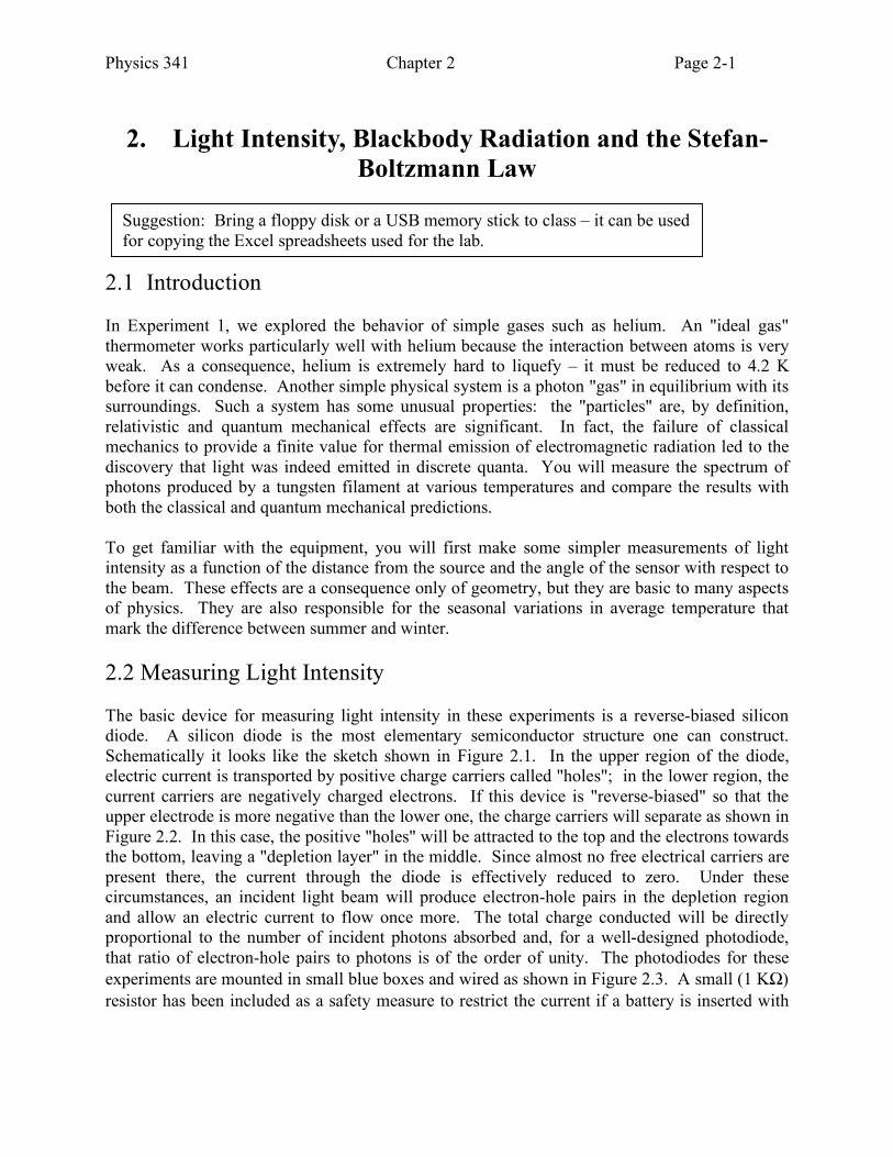
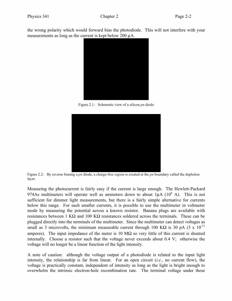
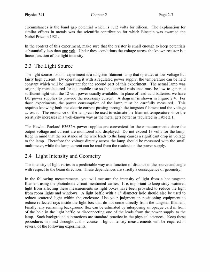
2.1 Introduction In Experiment 1, we explored the behavior of simple gases such as helium. An "ideal gas" thermometer works particularly well with helium because the interaction between atoms is very weak. As a consequence, helium is extremely hard to liquefy – it must be reduced to 4.2 K before it can condense. Another simple physical system is a photon "gas" in equilibrium with its surroundings. Such a system has some unusual properties: the "particles" are, by definition, relativistic and quantum mechanical effects are significant. In fact, the failure of classical mechanics to provide a finite value for thermal emission of electromagnetic radiation led to the discovery that light was indeed emitted in discrete quanta. You will measure the spectrum of photons produced by a tungsten filament at various temperatures and compare the results with both the classical and quantum mechanical predictions. To get familiar with the equipment, you will first make some simpler measurements of light intensity as a function of the distance from the source and the angle of the sensor with respect to the beam. These effects are a consequence only of geometry, but they are basic to many aspects of physics. They are also responsible for the seasonal variations in average temperature that mark the difference between summer and winter. 2.2 Measuring Light Intensity The basic device for measuring light intensity in these experiments is a reverse-biased silicon diode. A silicon diode is the most elementary semiconductor structure one can construct. Schematically it looks like the sketch shown in Figure 2.1. In the upper region of the diode, electric current is transported by positive charge carriers called "holes"; in the lower region, the current carriers are negatively charged electrons. If this device is "reverse-biased" so that the upper electrode is more negative than the lower one, the charge carriers will separate as shown in Figure 2.2. In this case, the positive "holes" will be attracted to the top and the electrons towards the bottom, leaving a "depletion layer" in the middle. Since almost no free electrical carriers are present there, the current through the diode is effectively reduced to zero. Under these circumstances, an incident light beam will produce electron-hole pairs in the depletion region and allow an electric current to flow once more. The total charge conducted will be directly proportional to the number of incident photons absorbed and, for a well-designed photodiode, that ratio of electron-hole pairs to photons is of the order of unity. The photodiodes for these experiments are mounted in small blue boxes and wired as shown in Figure 2.3. A small (1 KΩ) resistor has been included as a safety measure to restrict the current if a battery is inserted with
Suggestion: Bring a floppy disk or a USB memory stick to class – it can be used for copying the Excel spreadsheets used for the lab.
Physics 341 Chapter 2 Page 2-2
the wrong polarity which would forward bias the photodiode. This will not interfere with your measurements as long as the current is kept below 200 µA.
Figure 2.1: Schematic view of a silicon pn diode
Figure 2.2: By reverse biasing a pn diode, a charge-free region is created at the pn boundary called the depletion layer. Measuring the photocurrent is fairly easy if the current is large enough. The Hewlett-Packard 974As multimeters will operate well as ammeters down to about 1µA (106 A). This is not sufficient for dimmer light measurements, but there is a fairly simple alternative for currents below this range. For such smaller currents, it is possible to use the multimeter in voltmeter mode by measuring the potential across a known resistor. Banana plugs are available with resistances between 1 KΩ and 100 KΩ resistances soldered across the terminals. These can be plugged directly into the terminals of the multimeter. Since the multimeter can detect voltages as small as 3 microvolts, the minimum measurable current through 100 KΩ is 30 pA (3 x 10-11 amperes). The input impedance of the meter is 10 MΩ so very little of this current is shunted internally. Choose a resistor such that the voltage never exceeds about 0.4 V; otherwise the voltage will no longer be a linear function of the light intensity. A note of caution: although the voltage output of a photodiode is related to the input light intensity, the relationship is far from linear. For an open circuit (i.e., no current flow), the voltage is practically constant, independent of intensity as long as the light is bright enough to overwhelm the intrinsic electron-hole recombination rate. The terminal voltage under these
Physics 341 Chapter 2 Page 2-3
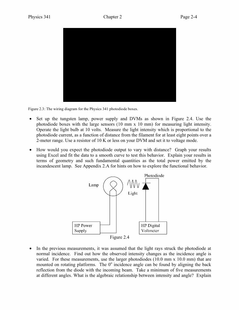
circumstances is the band gap potential which is 1.12 volts for silicon. The explanation for similar effects in metals was the scientific contribution for which Einstein was awarded the Nobel Prize in 1921. In the context of this experiment, make sure that the resistor is small enough to keep potentials substantially less than one volt. Under these conditions the voltage across the known resistor is a linear function of the light intensity 2.3 The Light Source The light source for this experiment is a tungsten filament lamp that operates at low voltage but fairly high current. By operating it with a regulated power supply, the temperature can be held constant which will be important for the second part of this experiment. The actual lamp was originally manufactured for automobile use so the electrical resistance must be low to generate sufficient light with the 12 volt power usually available. In place of lead-acid batteries, we have DC power supplies to provide the necessary current. A diagram is shown in Figure 2.4. For those experiments, the power consumption of the lamp must be carefully measured. This requires knowing both the electric current passing through the tungsten filament and the voltage across it. The resistance of the lamp can be used to estimate the filament temperature since the resistivity increases in a well-known way as the metal gets hotter as tabulated in Table 2.1. The Hewlett-Packard E3632A power supplies are convenient for these measurements since the output voltage and current are monitored and displayed. Do not exceed 13 volts for the lamp. Keep in mind that the resistance of the wire leads to the lamp causes a significant drop in voltage to the lamp. Therefore the voltage directly across the lamp should be measured with the small multimeter, while the lamp current can be read from the readout on the power supply. 2.4 Light Intensity and Geometry The intensity of light varies in a predictable way as a function of distance to the source and angle with respect to the beam direction. These dependences are strictly a consequence of geometry. In the following measurements, you will measure the intensity of light from a hot tungsten filament using the photodiode circuit mentioned earlier. It is important to keep stray scattered light from affecting these measurements so light boxes have been provided to reduce the light from room lights and windows. A light baffle with a 1" diameter hole should also be used to reduce scattered light within the enclosure. Use your judgment in positioning equipment to reduce reflected rays inside the light box that do not come directly from the tungsten filament. Finally, any remaining background flux can be estimated by interposing an opaque card in front of the hole in the light baffle or disconnecting one of the leads from the power supply to the lamp. Such background subtractions are standard practice in the physical sciences. Keep these procedures in mind throughout this course – light intensity measurements will be required in several of the following experiments.
Physics 341 Chapter 2 Page 2-4
Figure 2.3: The wiring diagram for the Physics 341 photodiode boxes.
• Set up the tungsten lamp, power supply and DVMs as shown in Figure 2.4. Use the photodiode boxes with the large sensors (10 mm x 10 mm) for measuring light intensity. Operate the light bulb at 10 volts. Measure the light intensity which is proportional to the photodiode current, as a function of distance from the filament for at least eight points over a 2-meter range. Use a resistor of 10 K or less on your DVM and set it to voltage mode.
• How would you expect the photodiode output to vary with distance? Graph your results using Excel and fit the data to a smooth curve to test this behavior. Explain your results in terms of geometry and such fundamental quantities as the total power emitted by the incandescent lamp. See Appendix 2.A for hints on how to explore the functional behavior.
Figure 2.4
• In the previous measurements, it was assumed that the light rays struck the photodiode at
normal incidence. Find out how the observed intensity changes as the incidence angle is varied. For these measurements, use the larger photodiodes (10.0 mm x 10.0 mm) that are mounted on rotating platforms. The 0o incidence angle can be found by aligning the back reflection from the diode with the incoming beam. Take a minimum of five measurements at different angles. What is the algebraic relationship between intensity and angle? Explain
Physics 341 Chapter 2 Page 2-5
why this occurs. The dependence of illumination on angle is the chief cause of seasonal variations in temperature. The Earth's spin axis is tilted by 23.4o with respect to the Earth's orbital plane around the Sun. Ann Arbor is located 42.4o north of the Equator. Calculate the angle of the Sun's rays with respect to the surface normal at noon in mid-summer and mid-winter. From this, find the corresponding ratio of average light intensity between the two seasons.
• An overwhelming majority of atmospheric scientists believe that the current level of fossil fuel burning is leading to global climate changes that will have very unpleasant impacts on our lives. The alternative sources of power are either nuclear fission or solar energy, either used directly or via secondary effects such as wind or waves. Direct conversion of solar to electric power using silicon photovoltaic devices similar to the sensors in this experiment might eventually become an economical solution. To estimate the area of silicon cells required, measure the open circuit voltage and short circuit current (set DVM scale to 500 mA) of the sample solar cells when exposed to direct sunlight (use the small DVMs and clip leads to attach to meter test probes). The value of the cell internal resistance, RI, is given by the ratio, Vopen circuit /I short circuit. The maximum power is extracted by a load resistance RL when the product of the voltage across the load times the current through it (VLIL) is a maximum. (NOTE: This is always less than V open circuit I short circuit ). Measure VL vs. load resistance. A resistor switch box is available for this purpose. Plot the power VL
2/RL vs. RL. From this graph, estimate the maximum power that the solar cell can deliver to a load, and the value of the load resistance for this.
• The average American consumes about 1 kilowatt. How large an area covered by solar cells
would this require? The US Census Bureau claims that the US population was 292,287,454 on January 1, 2004 (http://www.census.gov/). In the US, how many square meters would be needed to provide this power?
2.5 Blackbody Radiation and the Stefan-Boltzmann Law The origins of quantum mechanics arose from the failure of classical methods to explain the spectral distribution of light from hot objects. The experimental model system is a hot cavity such as an oven with walls at a uniform temperature T. A small hole is cut into an oven wall to allow a small fraction of the electromagnetic energy to escape. Such light is called blackbody radiation. Statistical mechanics plus classical electromagnetism predicted a spectral distribution called the Rayleigh-Jeans law that can be written as:
dI
df=2!f
2
c2kT (2.1)
where I is the intensity (power per unit area) of light emitted per unit frequency at frequency f by an object at temperature T. Although the derivation of this formula is beyond the scope of this course, the form can be easily explained. In classical statistical mechanics, every possible degree of freedom should acquire an average energy of
1
2kT. For example, a monatomic gas molecule
has energy
3
2kT because it can move in three independent directions. The number of independent
modes of oscillation in a cavity scales like f2 for reasons similar to the relationship of the area of
Physics 341 Chapter 2 Page 2-6
a sphere to its radius. The total intensity at a given frequency is the product of the number of modes available and the average energy in each. This is the physical content of Equation 2.1.
From a theoretical point of view, Equation 2.1 is a disaster. As the frequency f becomes large, the predicted intensity increases without limit, even for objects at modest temperature. This is called "the ultraviolet catastrophe". On the other hand, at low frequencies, the formula gave accurate predictions of experimental results, indicating that at least some aspects were basically correct. The problem was solved in two steps. Since Equation 2.1 leads to an infinite radiation rate, another approach must be found to compute the total energy emitted by a hot object. Ludwig Boltzmann found a thermodynamic argument to show that the total intensity is given by:
I = !T4 (2.2)
where σ is a constant of nature and T is the absolute temperature. This agreed with earlier experimental measurements by Josef Stefan. Equation 2.2 is called the Stefan-Boltzmann Law. The unusually rapid increase in radiation with temperature is a consequence of the massless nature of photons, the carriers of electromagnetic energy (the same kind of behavior governs phonons, the quanta of acoustic energy in solids and liquids). Although this relationship describes the total energy emitted, it does not predict the spectral distribution. That step was taken by Max Planck who postulated that electromagnetic energy was emitted in discrete units or quanta, each with energy given by hf where h is the Planck constant, 6.6256 x 10⁻³⁴ joule-second (see Table 2.4). For photon energies with hf>kT, it would no longer be possible to populate each mode with kT average energy since a fraction of hf is no longer allowed. The consequence is an additional factor of
hf /kT
ehf / kT
!1
that reduces the spectral distribution given by Equation 2.1. This factor approaches unity for small f, preserving the long wavelength Rayleigh-Jeans behavior but squelches the ultra-violet divergence. The result is the Planck spectral distribution:
dI
df=2!hf
3
c2
1
ehf / kT
"1 (2.3)
By integrating this equation over all frequencies, one can recover Equation 2.2 and, in addition, find that the constant, σ, is explicitly given by:
! =2"
5k4
15h3c2
= 5.67 #10$8W /m
2%K
4 (2.4)
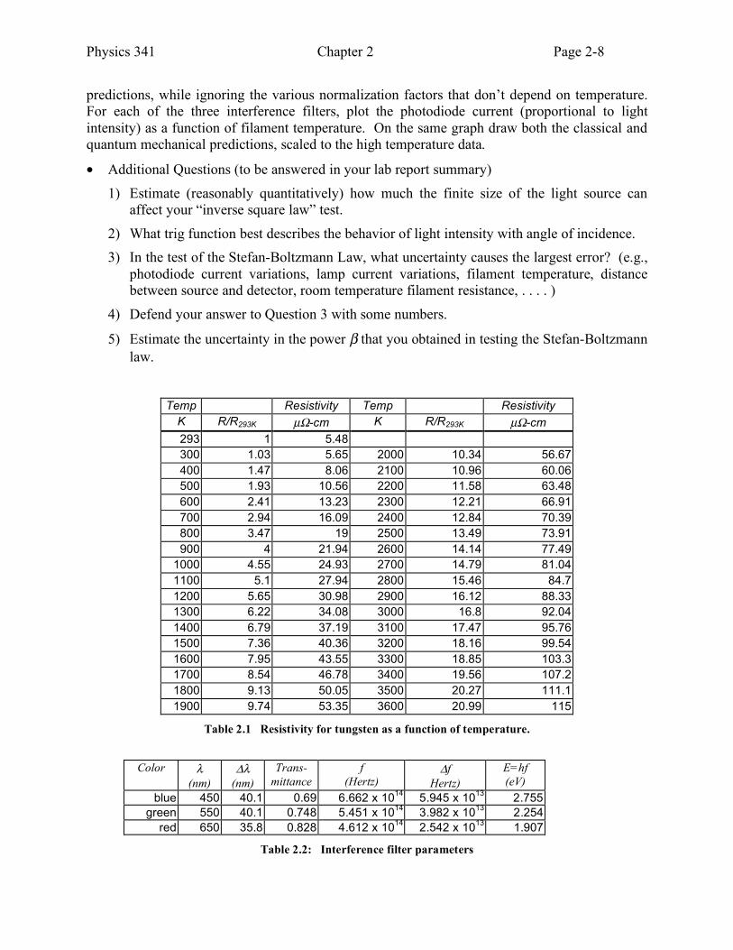
• Verify the Stefan-Boltzmann Law by measuring the intensity radiated as a function of filament temperature. The temperature can be inferred from the lamp resistance and the resistivity data tabulated in Table 2.1. For these purposes, the room temperature resistance can most accurately be obtained with the Hewlett-Packard multimeter operating in ohmmeter mode. The filament resistance is very small, so be sure to subtract the resistance of the ohmmeter leads. The tabular values contained in Table 2.1 have been entered into an Excel spreadsheet file. With
Physics 341 Chapter 2 Page 2-7
these data you can use Excel to interpolate temperature automatically from your current and voltage measurements. The intensity emitted can be calculated from the total electric power dissipated by the lamp. You will also need to find out the surface area of the filament responsible for the light emission. Two quantities must be determined: the wire diameter or radius and its length. The length is hard to measure because the filament is tightly coiled, but it can be computed from the room temperature resistance, R, the wire radius, r, and the formula:
R = !!
"r2 (2.5)
where ρ is the resistivity given in Table 2,1 and ! is the wire length. You will need to measure the filament wire radius of a similar lamp dissected to expose the tungsten wire. A micrometer is available for this purpose. Using Equation 2.5, you can then find the emitting area,
A = 2!r! . The intensity, I, at the surface of the tungsten is the total electrical power iV divided by the area,
I =iV
A (2.6)
where i is the current through the lamp, V is the potential across the lamp and A is the area you have derived from the above. Note that the V here is not exactly equal to the voltage read off the of the power supply meter. Take data with power supply voltages from about 4 V to 13 V in steps of 1 V. Plot the intensity radiated as a function of temperature. Fit your data to
I = !T " using Excel and determine the constants α and β. Compare your experimental results with the theoretical values. You will find that the fit is poor at lower filament temperatures due to the temperature non-uniformity in the filament as you can see by inspection. Feel free to drop a few low temperature points to improve the fit. For these measurements, you can operate the filament up to 13.0 volts. Use the Trendline function of Excel to find the power law behavior of intensity as a function of temperature, or use the method of logarithmic derivatives as discussed in Appendix 2.A.
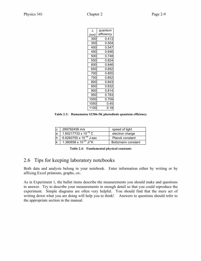
• Next investigate the Planck spectral distribution (Equation 2.3) for different filament temperatures. Use the photodiode boxes with the large sensors (10 mm x 10 mm) for this part of the measurement and a resistor of 10K or greater on the DVM to measure the photodiode current. To measure the light intensity at different frequencies, three interference filters are available with passbands at 450 nm (blue), 550 nm (green) and 650 nm (red). The bandwidth and transmission for each band are provided in Table 2.2. Handle the filters with care – please avoid getting fingerprints on the glass surfaces.
• Take photodiode current data at several filament voltages, e.g., 9 V, 11 V, and 13 V with each filter.
• Consult Appendix 2.B to determine how to calculate dI/df from the photodiode currents you have measured and the data provided in Tables 2.2 and 2.3. Plot dI/df vs f for each filament temperature along with the Planck and Rayleigh-Jeans predictions for dI/df. [You may have to scale the classical prediction by an appropriate factor to get it on the same graph!]
• The Planck spectral distribution (Equation 2.3) gives distinctly different predictions than the classical Rayleigh-Jeans law (Equation 2.1). In one case, the temperature dependence is given by
1/(ehf / kT
!1), whereas the latter predicts a simple linear behavior. You can compare the shape of the photodiode current vs. temperature curve with the quantum mechanical and classical
Physics 341 Chapter 2 Page 2-8
predictions, while ignoring the various normalization factors that don’t depend on temperature. For each of the three interference filters, plot the photodiode current (proportional to light intensity) as a function of filament temperature. On the same graph draw both the classical and quantum mechanical predictions, scaled to the high temperature data.
• Additional Questions (to be answered in your lab report summary)
1) Estimate (reasonably quantitatively) how much the finite size of the light source can affect your “inverse square law” test.
2) What trig function best describes the behavior of light intensity with angle of incidence. 3) In the test of the Stefan-Boltzmann Law, what uncertainty causes the largest error? (e.g.,
photodiode current variations, lamp current variations, filament temperature, distance between source and detector, room temperature filament resistance, . . . . )
4) Defend your answer to Question 3 with some numbers.
5) Estimate the uncertainty in the power β that you obtained in testing the Stefan-Boltzmann law.
c 299792458 m/s speed of light e 1.60217733 x 10⁻¹⁹ C electron charge h 6.6260755 x 10⁻³⁴ J-sec Planck constant k 1.380658 x 10⁻²³ J/°K Boltzmann constant
Table 2.4: Fundamental physical constants
2.6 Tips for keeping laboratory notebooks Both data and analysis belong in your notebook. Enter information either by writing or by affixing Excel printouts, graphs, etc. As in Experiment 1, the bullet items describe the measurements you should make and questions to answer. Try to describe your measurements in enough detail so that you could reproduce the experiment. Simple diagrams are often very helpful. You should find that the mere act of writing down what you are doing will help you to think! Answers to questions should refer to the appropriate section in the manual.
Physics 341 Chapter 2 Page 2-10
Appendix 2.A Extracting Power Law Behavior from Data Power law behavior frequently occurs in physics. In this experiment, one expects to find that light intensity varies as R2 and the radiated power from a hot filament varies as T4. It would be nice to have a systematic way of testing your data to see what exponents are actually measured. Assume we have a power law relationship:
y = xp The logarithmic derivative is defined by:
d log y
d log x=x
y
dy
dx=x
xp! px
p"1= p (2.8)
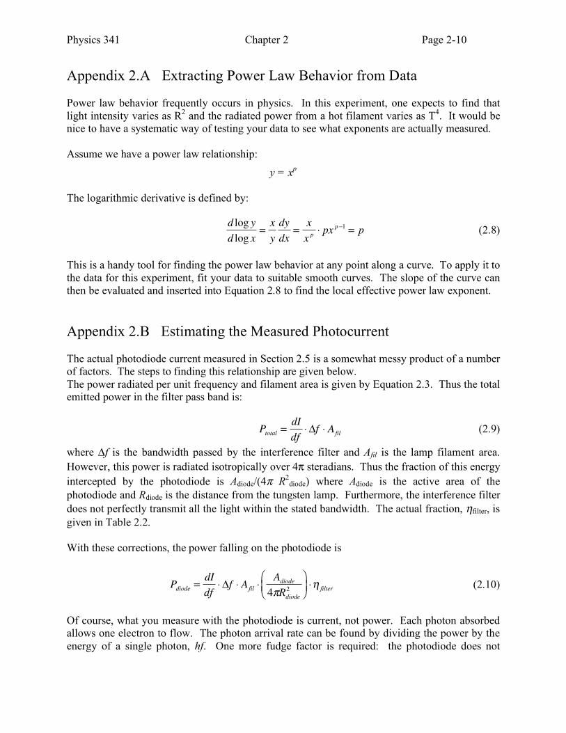
This is a handy tool for finding the power law behavior at any point along a curve. To apply it to the data for this experiment, fit your data to suitable smooth curves. The slope of the curve can then be evaluated and inserted into Equation 2.8 to find the local effective power law exponent. Appendix 2.B Estimating the Measured Photocurrent The actual photodiode current measured in Section 2.5 is a somewhat messy product of a number of factors. The steps to finding this relationship are given below. The power radiated per unit frequency and filament area is given by Equation 2.3. Thus the total emitted power in the filter pass band is:
Ptotal =dI
df! "f ! Afil (2.9)
where Δf is the bandwidth passed by the interference filter and Afil is the lamp filament area. However, this power is radiated isotropically over 4π steradians. Thus the fraction of this energy intercepted by the photodiode is Adiode/(4π R2
diode) where Adiode is the active area of the photodiode and Rdiode is the distance from the tungsten lamp. Furthermore, the interference filter does not perfectly transmit all the light within the stated bandwidth. The actual fraction, ηfilter, is given in Table 2.2. With these corrections, the power falling on the photodiode is
Pdiode =dI
df! "f ! Afil !
Adiode
4#Rdiode
2
$
% &
'
( ) !* filter (2.10)
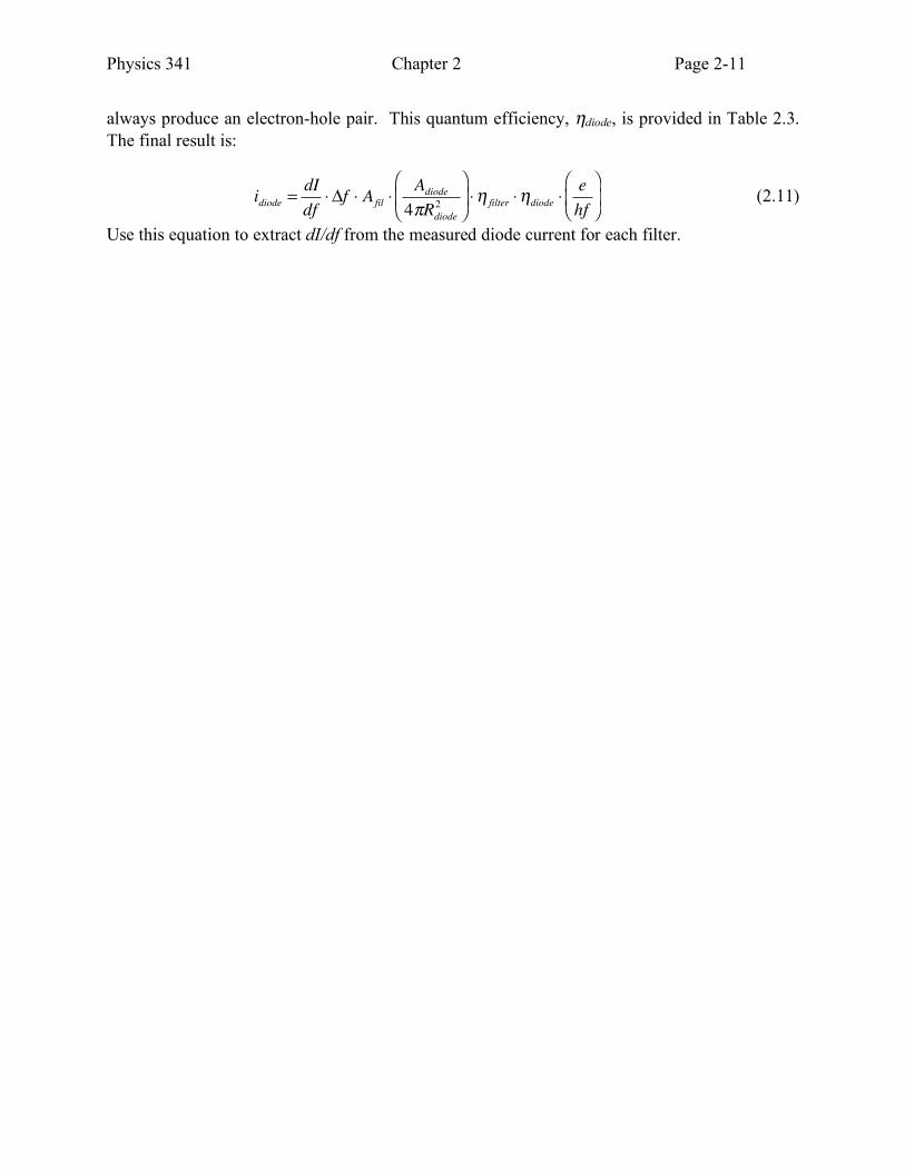
Of course, what you measure with the photodiode is current, not power. Each photon absorbed allows one electron to flow. The photon arrival rate can be found by dividing the power by the energy of a single photon, hf. One more fudge factor is required: the photodiode does not
Physics 341 Chapter 2 Page 2-11
always produce an electron-hole pair. This quantum efficiency, ηdiode, is provided in Table 2.3. The final result is:
idiode =dI
df! "f ! Afil !
Adiode
4#Rdiode
2
$
% &
'
( ) !* filter !*diode !
e
hf
$
% &
'
( ) (2.11)
Use this equation to extract dI/df from the measured diode current for each filter.
Physics 341 Chapter 2 Page 2-12
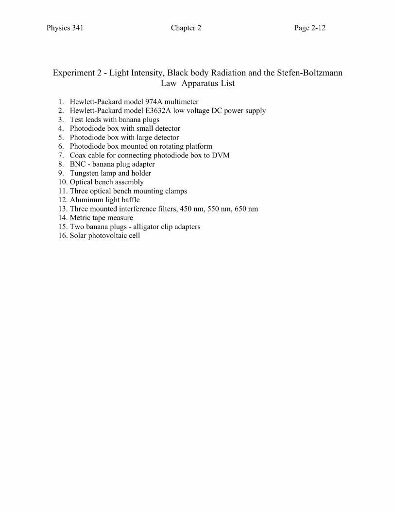
Experiment 2 - Light Intensity, Black body Radiation and the Stefen-Boltzmann Law Apparatus List
1. Hewlett-Packard model 974A multimeter 2. Hewlett-Packard model E3632A low voltage DC power supply 3. Test leads with banana plugs 4. Photodiode box with small detector 5. Photodiode box with large detector 6. Photodiode box mounted on rotating platform 7. Coax cable for connecting photodiode box to DVM 8. BNC - banana plug adapter 9. Tungsten lamp and holder 10. Optical bench assembly 11. Three optical bench mounting clamps 12. Aluminum light baffle 13. Three mounted interference filters, 450 nm, 550 nm, 650 nm 14. Metric tape measure 15. Two banana plugs - alligator clip adapters 16. Solar photovoltaic cell