2. Linear Equations2. Linear Equations

Objectives:

1. Introduction to Gaussian Elimination.

2. Using multiple row operations.

3. Exercise - let’s see if you can do it.

Refs: B & Z 4.2, 4.3.

Example 1 (revisited):

constant

€

3 −1 −2

1 1 6

⎡

⎣ ⎢

⎤

⎦ ⎥

x y

€

R1 → R2

€

R2 → R1

Use operation (A)

€

R2 − 3R1 → R2

Use operation (C)

€

−1 4 R2 → R2

Use operation (B)€

1 1 6

3 −1 −2

⎡

⎣ ⎢

⎤

⎦ ⎥~

€

1 1 6

0 −4 −20

⎡

⎣ ⎢

⎤

⎦ ⎥~

€

1 1 6

0 1 5

⎡

⎣ ⎢

⎤

⎦ ⎥~

€

1 0 1

0 1 5

⎡

⎣ ⎢

⎤

⎦ ⎥~

€

R1 − R2 → R1

Use operation (C)

Bingo! Read off solution.

x y constant

Solution: x=1 y=5

We have just used a procedure known as Gaussian elimination (or row reduction) which transforms a matrix

The procedure also applies to larger matrices.

€

a b e

c d g

⎡

⎣ ⎢

⎤

⎦ ⎥

into

€

1 0 h

0 1 i

⎡

⎣ ⎢

⎤

⎦ ⎥

Example 2:

Solve for x, y and z:

€

2x + y − 4z = 3

x − 2y + 3z = 4

−3x + 4y − z = −2.

The first step is to construct the augmented matrix:

€

2 1 −4 3

1 −2 3 4

−3 4 −1 −2

⎡

⎣

⎢ ⎢ ⎢

⎤

⎦

⎥ ⎥ ⎥€

← equation 1

€

← equation 2

€

← equation 3

x coefficientsconstant terms

z coefficientsy coefficients

Our aim is to produce an equivalent augmented matrix which has 1’s on the diagonal and zeroes elsewhere (onthe LHS).

€

2 1 −4 3

1 −2 3 4

−3 4 −1 −2

⎡

⎣

⎢ ⎢ ⎢

⎤

⎦

⎥ ⎥ ⎥

€

1 −2 3 4

0 5 −10 −5

−3 4 −1 −2

⎡

⎣

⎢ ⎢ ⎢

⎤

⎦

⎥ ⎥ ⎥

~

~

€

1 −2 3 4

2 1 −4 3

−3 4 −1 −2

⎡

⎣

⎢ ⎢ ⎢

⎤

⎦

⎥ ⎥ ⎥

2

€

R1 → R2

€

R2 → R1

Use (A) to get a 1 in the top left corner

€

R2 − 2R1 → R2

Use (C) to get a 0 in the position indicated

€

R3 + 3R1 → R3 Use (C) to get a 0 in the bottom left position

€

R1 + 2R2 → R1

Use (C) to get a 0 in the positionindicated

€

R3 + 2R2 → R3

Use (C) to get a 0 in the position indicated

€

14 R3 → R3 Use (B) to get a 1 in the

bottom right corner

~

€

1 0 −1 2

0 1 −2 −1

0 −2 8 10

⎡

⎣

⎢ ⎢ ⎢

⎤

⎦

⎥ ⎥ ⎥-2

~

€

1 0 −1 2

0 1 −2 −1

0 0 4 8

⎡

⎣

⎢ ⎢ ⎢

⎤

⎦

⎥ ⎥ ⎥4

Use (B) to get a 1 in the centre

€

15 R2 → R2

€

1 −2 3 4

0 1 −2 −1

0 −2 8 10

⎡

⎣

⎢ ⎢ ⎢

⎤

⎦

⎥ ⎥ ⎥

-2~€

1 −2 3 4

0 5 −10 −5

0 −2 8 10

⎡

⎣

⎢ ⎢ ⎢

⎤

⎦

⎥ ⎥ ⎥

5~

Solution:

€

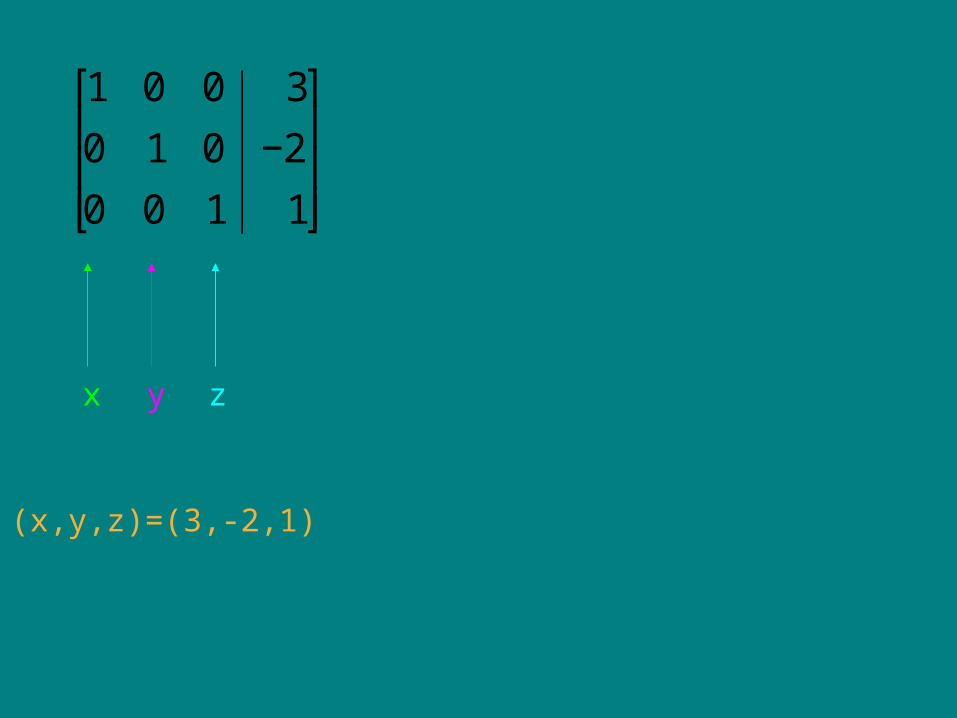
x = 4, y = 3, z = 2.

Always substitute these values back into ALL of your equations to check your solution.

Note: It is very easy to make algebraic mistakes!!!

€

1 0 0 4

0 1 −2 −1

0 0 1 2

⎡

⎣

⎢ ⎢ ⎢

⎤

⎦

⎥ ⎥ ⎥

-2~

€

1 0 0 4

0 1 0 3

0 0 1 2

⎡

⎣

⎢ ⎢ ⎢

⎤

⎦

⎥ ⎥ ⎥

~

€

R2 + 2R3 → R2Use (C) to get a 0 in the position indicated

We now have the required form

x constantzy

€

1 0 −1 2

0 1 −2 −1

0 0 1 2

⎡

⎣

⎢ ⎢ ⎢

⎤

⎦

⎥ ⎥ ⎥

~

€

R1 + R3 → R1Use (C) to get a 0 in the Top right corner

Check:

€

2x + y − 4z = 3

x − 2y + 3z = 4

−3x + 4y − z = −2,

x = 4, y = 3, z = 2?

€

1. 2(4)+ (3) − 4(2)

= 8 + 3− 8 = 3

€

2. 4 − 2(3)+ 3(2)

= 4 − 6 + 6 = 4

€

3. − 3(4)+ 4(3) − 2

= −12 +12 − 2 = −2.

Using multiple operationsWe can alter more than one row at a time to speed up the Gaussian elimination procedure.

Example 3:

€

4 2 8

9 3 6

⎡

⎣ ⎢

⎤

⎦ ⎥

€

4 2 8

9 3 6

⎡

⎣ ⎢

⎤

⎦ ⎥

€

2 1 4

9 3 6

⎡

⎣ ⎢

⎤

⎦ ⎥~

€

2 1 4

3 1 2

⎡

⎣ ⎢

⎤

⎦ ⎥~

€

2 1 4

3 1 2

⎡

⎣ ⎢

⎤

⎦ ⎥~

€

12 R1 → R1

€

13 R2 → R2

€

12 R1 → R1

€

13 R2 → R2

No problem - we have saved some time.(Here we are using multiple (B)Operations)

Example 4:

We can perform multiple (C ) operations provided at least one row is kept constant and only multiples of it are used to perform the other operations.

€

1 2 −2 4

3 1 0 −1

2 2 −1 0

⎡

⎣

⎢ ⎢ ⎢

⎤

⎦

⎥ ⎥ ⎥

€

1 2 −2 4

0 −5 6 −13

2 2 −1 0

⎡

⎣

⎢ ⎢ ⎢

⎤

⎦

⎥ ⎥ ⎥

~

€

1 2 −2 4

0 −5 6 −13

0 −2 3 −8

⎡

⎣

⎢ ⎢ ⎢

⎤

⎦

⎥ ⎥ ⎥

~

€

R2 − 3R1 → R2

€

R3 − 2R1 → R3

Obviously, performing multiple (A) type operations causes no problem.

Exercise 1: Solve the following system of simultaneous equations:

€

2x + 4y − z = −3

x − 3y + 2z =11

4x − 2y + 5z = 21.

Example 4 (continued):

€

1 2 −2 4

3 1 0 −1

2 2 −1 0

⎡

⎣

⎢ ⎢ ⎢

⎤

⎦

⎥ ⎥ ⎥

€

R3 − 2R1 → R3

€

R2 − 3R1 → R2

€

1 2 −2 4

0 −5 6 −13

0 −2 3 −8

⎡

⎣

⎢ ⎢ ⎢

⎤

⎦

⎥ ⎥ ⎥

~No problem -We kept R1 constantAnd used it to get R2 and R3

Solution to Exercise

€

2 4 −1 −3

1 −3 2 11

⎡

⎣

⎢ ⎢ ⎢

⎤

⎦

⎥ ⎥ ⎥

€

⎡

⎣

⎢ ⎢ ⎢

⎤

⎦

⎥ ⎥ ⎥

€

2 4 −1 −3 ⎡

⎣

⎢ ⎢ ⎢

⎤

⎦

⎥ ⎥ ⎥

€

2 4 −1 −3

1 −3 2 11

4 −2 5 21

⎡

⎣

⎢ ⎢ ⎢

⎤

⎦

⎥ ⎥ ⎥€

R1 → R2

€

R2 → R1

€

R2 − 2R1 → R2

€

R3 − 4R1 → R3

€

R2 10 → R2

€

R3 2 → R3

€

R3 −10R2 → R3€

R1 + 3R2 → R1

€

€

R1 −1 2 R3 → R1

€

R2 +1 2 R3 → R2

€

1 −3 2 11

2 4 −1 −3

4 −2 5 21

⎡

⎣

⎢ ⎢ ⎢

⎤

⎦

⎥ ⎥ ⎥

~

€

1 −3 2 11

0 10 −5 −25

0 10 −3 −23

⎡

⎣

⎢ ⎢ ⎢

⎤

⎦

⎥ ⎥ ⎥

~

€

1 0 1 2 7 2

0 1 −1 2 −5 2

0 0 1 1

⎡

⎣

⎢ ⎢ ⎢

⎤

⎦

⎥ ⎥ ⎥

~€

1 0 1 2 7 2

0 1 −1 2 −5 2

0 0 2 2

⎡

⎣

⎢ ⎢ ⎢

⎤

⎦

⎥ ⎥ ⎥

~€

1 −3 2 11

0 1 −1 2 −5 2

0 10 −3 −23

⎡

⎣

⎢ ⎢ ⎢

⎤

⎦

⎥ ⎥ ⎥

~

€

1 0 0 3

0 1 0 −2

0 0 1 1

⎡

⎣

⎢ ⎢ ⎢

⎤

⎦

⎥ ⎥ ⎥

x y z

(x,y,z)=(3,-2,1)

You can now attempt

Q1 and Q2 from Exercise Sheet 1

of the Orange Book