2 Literature review - Open Access Repository · 2 Literature review This chapter discusses the...

2 Literature review

This chapter discusses the general work in artificial intelligence which leads to machine

learning and classifier learning. It then concentrates on the areas of multiple classifier

learning, which is relevant to the subsetting algorithm in chapter 3, and Haar Classifier

Cascades for object detection, which are built upon in chapters 5, 6 and 7.

2.1 Machine learning

Machine learning has been defined as ‘the study of computer algorithms that improve

automatically through experience’ (Mitchell, 1997). An algorithm has ‘learnt’ if it finds

a pattern in its past experience that is useful in its future. General surveys of machine

learning are given in (Langley, 1996; Mitchell, 1997; Witten & Frank, 2005b). This

thesis concentrates on the part of machine learning called ‘classifier learning’.

2.2 Introduction to classifier learning

Many learners generate classifiers: algorithms that can take an input instance contain-

ing several attribute values and output the class that instance belongs to. Classifier

learning is more versatile than it may first appear – some examples of problems de-

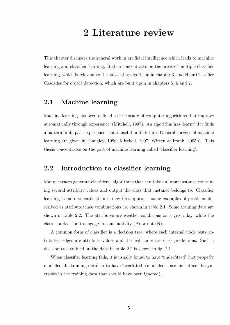
scribed as attribute/class combinations are shown in table 2.1. Some training data are

shown in table 2.2. The attributes are weather conditions on a given day, while the

class is a decision to engage in some activity (P) or not (N).

A common form of classifier is a decision tree, where each internal node tests at-

tributes, edges are attribute values and the leaf nodes are class predictions. Such a

decision tree trained on the data in table 2.2 is shown in fig. 2.1.

When classifier learning fails, it is usually found to have ‘underfitted’ (not properly

modelled the training data) or to have ‘overfitted’ (modelled noise and other idiosyn-

crasies in the training data that should have been ignored).

5

Chapter 2 Literature review 6

Table 2.1: Example classifier learning applications

Attributes Class Source

Image of road from front of car Which way to turn (Pomerleau, 1989)

Credit applicant’s details Whether to extend

credit

(Michie, 1989)

Words, phrases and header in-

formation in e-mail

Whether e-mail is

‘spam’

(Sahami et al., 1998)


Table 2.2: Example classifier training data (Quinlan, 1986)

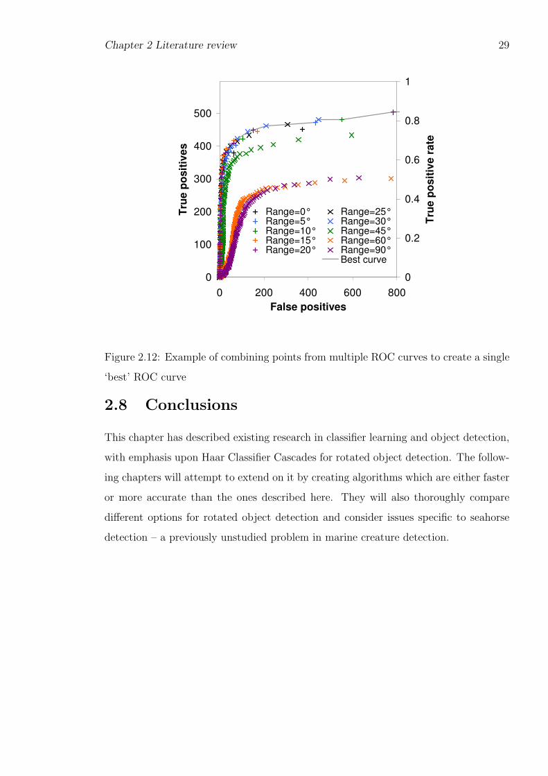
Figure 2.1: Example decision tree (Quinlan, 1986)


2.3 Multiple classifier learning

Individual classifier learners may not be able to create a close model of their training

data. Some, such as decision tree learners, can find a close match, but only at the

expense of creating a very complex (and probably overfitted) tree. Even so, there

are ways to create many small decision trees, or several completely di!erent types of

classifiers, which together provide better accuracy and less overfitting than a single

classifier can achieve.

2.3.1 Bagging

Statisticians have been using a technique called ‘bootstrap sampling’ for many years.

One application of this in machine learning is ‘bootstrap aggregating’ or ‘bagging’

(Breiman, 1996).

The impetus comes from the statistical ideal of having many training examples.

Unfortunately, su"ciently large data sets are frequently expensive or impossible to

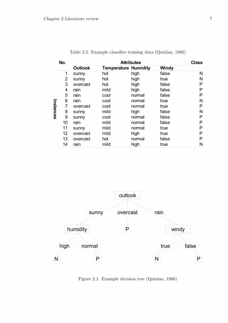
obtain. In bootstrap sampling, multiple random samples are created from the source

data by sampling with replacement. This is illustrated in fig. 2.2. Samples may overlap

or contain duplicate items, yet the results (when combined) are usually more accurate

than a single sampling of the entire source data achieves.

The bootstrap samples may then be used to each train a classifier. If the train-

ing samples are di!erent as intended, the trained classifiers will (usually) be di!erent.

These classifiers can then classify new instances by each making a prediction and com-

bining predictions to give a final classification. Because it aggregates results from

classifiers trained on bootstrap samples, the overall technique is called ‘bootstrap ag-

gregating’.

Bagging is only useful if the classifiers are di!erent. This only happens if small

changes in the training data can result in large changes in the resulting classifier – that

is, if the learning method is unstable (Breiman, 1996).


Figure 2.2: Bootstrap sampling example: 3 bootstrap samples created from a 5-instance

dataset


2.3.2 Attribute subsetting

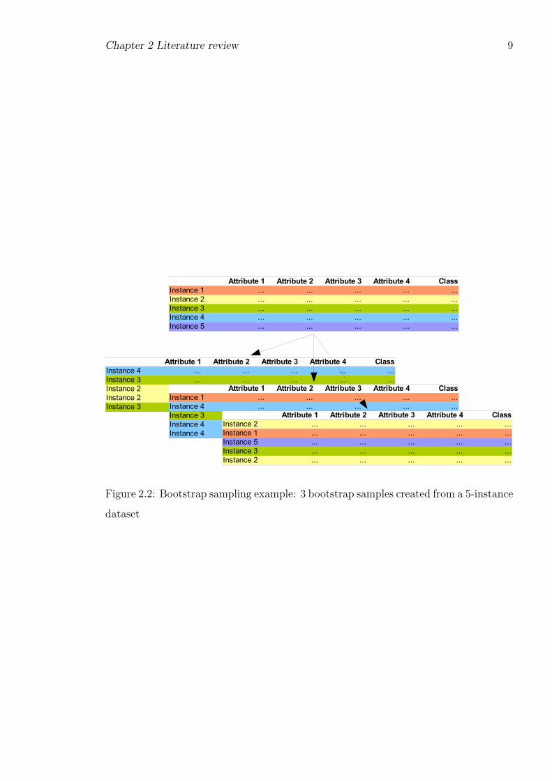
Attribute subsetting is a multiple classifier technique with some similarities to bagging.

Multiple training datasets are generated from the initial training data; each training

set contains all the instances from the original data, but some attributes are removed,

as illustrated in fig. 2.3. A classifier is then learnt on each training set. To classify a

new instance, predictions from each classifier are combined to give a final classification.

If the training data are stored in a table with each row representing an instance

and each column containing attribute values, bagged training samples are built by

selecting table rows (fig. 2.2), while attribute subsetted training samples are built by

selecting table columns (fig. 2.3). Because of this similarity, the technique has been

referred to as ‘attribute bagging’ (Bryll et al., 2003) and ‘feature bagging’ (Sutton

et al., 2005), terms which are only technically accurate if the attributes are sampled

with replacement. This has been tested (Bay, 1998), but did not significantly a!ect

accuracy.

Attribute subsetting has been e!ective when the base classifiers are neural networks

(Cherkauer, 1996), decision trees (Ho, 1998; Bryll et al., 2003), nearest-neighbour

classifiers (Bay, 1998) and conditional random fields (Sutton et al., 2005).

The virtual attribute subsetting algorithm in chapter 3 is able to gain some of the

benefits of attribute subsetting without needing the time to train additional classifiers,

but only works for certain types of base classifiers, as explained in section 3.2.2.

2.3.3 Stacking

There are many types of classifier, none of which has shown itself universally superior to

all others. This suggests that a good multiple classifier might take the output of several

individual classifiers of di!erent types and combine them. This is the idea behind

‘stacked generalization’, or ‘stacking’ (Wolpert, 1992). Each individual classifier is

called a ‘level-0 model’. Each may vote, or may have its output sent to a ‘level-1 model’

– another classifier that tries to learn which level-0 models are most reliable. Level-1

models are usually more accurate than simple voting, provided they are given the class

probability distributions from the level-0 models and not just the single predicted class

(Ting & Witten, 1997). The confidence measures in chapter 6 make similar use of

underlying numeric measurements.


Figure 2.3: Attribute subsetting example: 3 attribute subsets created from a 4-attribute

dataset

2.3.4 Boosting

If a classifier’s error on its training data is better than 50% but worse than 0%, it is

called a ‘weak’ classifier. A weak classifier learner is capable of learning ‘weak’ classifiers

only. A ‘strong’ classifier learner is capable of learning a classifier that comes arbitrarily

close to 0% error on its training data in polynomial time (Kearns & Vazirani, 1994).

The boosting process can obtain strong accuracy by iteratively training classifiers

with a weak learner. After training a classifier, it measures its accuracy on the training

data, emphasises the misclassified instances and trains a new classifier on the modified

dataset. At classification time, the boosting classifier combines the results from the

individual classifiers it trained.

Boosting was originally proposed by Schapire and Freund (Schapire, 1990; Freund,

1995). In their ‘Adaptive Boosting’ or ‘AdaBoost’ algorithm (Freund & Schapire,

1996), each of the training instances starts with a weight that tells the base classifier

its relative importance. If there are n instances, the starting weights are all 1n . The

individual classifier training algorithm must therefore be able to read and respond

to these weights, resulting in di!erent classifiers after each round of reweighting and

reclassification. Each classifier also receives a weight based on its accuracy; its output


at classification time is multiplied by this weight.

Freund and Schapire proved that, if the base classifier used by AdaBoost has an

error rate of just slightly less than 50%, the training error of the meta-classifier will

approach zero exponentially fast (Freund & Schapire, 1996). On a two-class problem,

such as the object detection problems of this thesis, the base classifier only needs to

be slightly better than chance to achieve this error rate. On problems with more than

two classes less than 50% error is harder to achieve. Boosting appears to be vulnerable

to overfitting; in tests, however, it rarely overfits excessively (Dietterich, 2000).

2.3.4.1 Boosting the margin

As boosting runs through multiple iterations, the boosted classifier’s error on both

training and testing data decreases rapidly; the training error may even decrease to zero.

If boosting continues past this point, its error on the test data may continue decreasing

(Quinlan, 1996). Schapire et al. suggested that this is because the combined classifiers’

‘margin’, or confidence in its output, continues increasing and that this in turn improves

testing accuracy (Schapire et al., 1997). This leads to boosting algorithms which

intentionally try to boost the margin; they can create more accurate classifiers (Schapire

& Singer, 1999), although they don’t always do so (Breiman, 1998; Reyzin & Schapire,

2006).

This is also relevant to the confidence measures made in chapter 6, which amount

to margin measurements made from a boosted classifier.

2.3.5 Implementation

Many standard classifier learners and meta-classification techniques are implemented in

the Waikato Environment for Knowledge Analysis (weka), a generic machine learning

toolkit (Witten & Frank, 2005b). The meta-classification experiments in chapter 3 and

the segment matching formula learning in chapter 7 were both carried out in weka.

2.4 Introduction to computer vision

Humans gain a great deal of information through vision, and there are many prob-

lems which computers could solve if they were similarly capable. Unfortunately, while


capturing and storing images on computers is trivial, deriving meaningful information

from them is not.

An example is the problem of content-based image retrieval. Usually, this involves

some user providing a keyword as a request for images described by that keyword, or

providing an image as a request for similar images. Image retrieval algorithms must

partition the images in their database into meaningful segments, as in (Belongie et al.,

1998), or derive features from the images which correlate with the users’ requests, as

in (Schmid & Mohr, 1997).

An extensively studied field within computer vision is face recognition: identifying

people from their appearance. This can involve finding very subtle geometry, which in

turn can be computationally expensive to locate. Given images containing faces (such

as sequences from a security camera), it is therefore best to detect face regions within

the image before running a recognition algorithm. This leads to the problem of face

detection, and its general case of object detection.

2.4.1 Object detection

An object detection algorithm takes a large image and should return all subregions of

that image representing objects of a given class. It should be fast and robust in doing

so; in the face detection application, the point is to save time by not running the face

recognition algorithm all over the image. If the face detector takes longer to run than

the face recognition algorithm needs to return a negative on non-face regions, the face

detection part is useless. Apart from face detection, common object detection tasks

include vehicle detection, such as (Papageorgiou & Poggio, 2000) and hand detection,

as in (Kolsch & Turk, 2004b).

2.4.1.1 Marine creature detection

Another object detection problem is that of finding marine animals in underwater

images or video sequences – a problem considered in detail in chapters 5, 6 and 7

of this thesis. This may be done for pose detection leading to behavioural analysis,

or as the first stage in measuring the size or mass of farmed fish (Lines et al., 2001;

Williams et al., 2006). Unlike faces in many environments, most marine creatures do

not consistently orient themselves within images, so a marine creature detector must


allow for creatures in many di!erent poses.

A related problem is marine species identification. Such an algorithm may only

identify creatures that have been caught and lined up for the camera (Chen et al.,

2005), or may identify freely-swimming fish and thus need to start with fish detection

(Semani et al., 2002).

2.5 Image features

Computer vision algorithms can often solve multiple problems. The Haar Wavelet

Features used in this thesis for object detection were used for image retrieval (Jacobs

et al., 1995) before being applied to pedestrian detection (Oren et al., 1997) and gen-

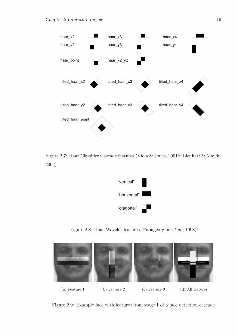
eralised to object detection (Papageorgiou et al., 1998). The features used by the Haar

Classifier Cascade algorithm were created for face detection (Viola & Jones, 2001b)

but were later used for face recognition (Jones & Viola, 2003b). The common ground

is the feature set – images can yield an enormous range of features, few of which are

likely to discriminate between the object to detect and everything else that may appear

in the image. Feature selection algorithms therefore receive a lot of attention.

One such method, the eigenface algorithm, finds features defining complete image

regions. It was originally created for face recognition (Turk & Pentland, 1991), but

is also e!ective at face detection (Popovici & Thiran, 2003). Two other well-known

feature types are SIFT (Scale-Invariant Feature Transform), usually used for object

recognition (Lowe, 1999), and Gabor Filters (Schiele & Crowley, 2000). There are also

regular classifier algorithms which have been successfully applied with input provided

directly from image pixel regions, such as neural networks (Rowley et al., 1998a).

The Haar Classifier Cascades studied in detail in this thesis use two-dimensional Haar

Wavelet Features: simple rectangular patterns of light and dark.

2.6 Haar Classifier Cascades

This approach to object detection was first proposed and implemented by Viola and

Jones (Viola & Jones, 2001b). An image region that may represent the object is

classified as described below and illustrated in fig. 2.4.


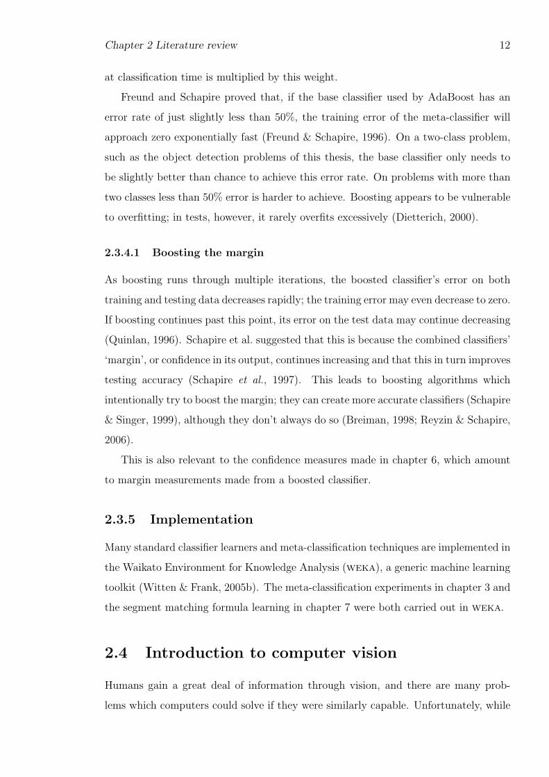
1. A cascade steps through several stages in turn; it stops and returns false if a stage

returns false. If all stages return true, the cascade returns true.

2. A stage returns true if the sum of its feature outputs exceeds a chosen threshold.

3. A feature returns the sum of its rectangle outputs.

4. A rectangle returns the sum of pixel values in the image region bounded by that

rectangle, multiplied by a chosen weight.

Figure 2.4: Haar Classifier Cascade classification process

Some details of Haar Classifier Cascade training or detection are implementation

dependent. Sometimes such details will be described with reference to Viola and Jones

for the original implementation (Viola & Jones, 2001b) or to Leinhardt and Maydt

for their extensions (Lienhart & Maydt, 2002). At other times, ‘OpenCV’ will be

mentioned; these are the libraries used as a starting point for the experiments in this

thesis, which are discussed further in section 2.6.8.

2.6.1 Rectangle calculation

Running one cascade across one image involves millions of rectangle measurements.

The time taken to return the sum of pixel values within a rectangle is therefore crucial.

This is done in constant time by precomputing, with a dynamic programming approach,

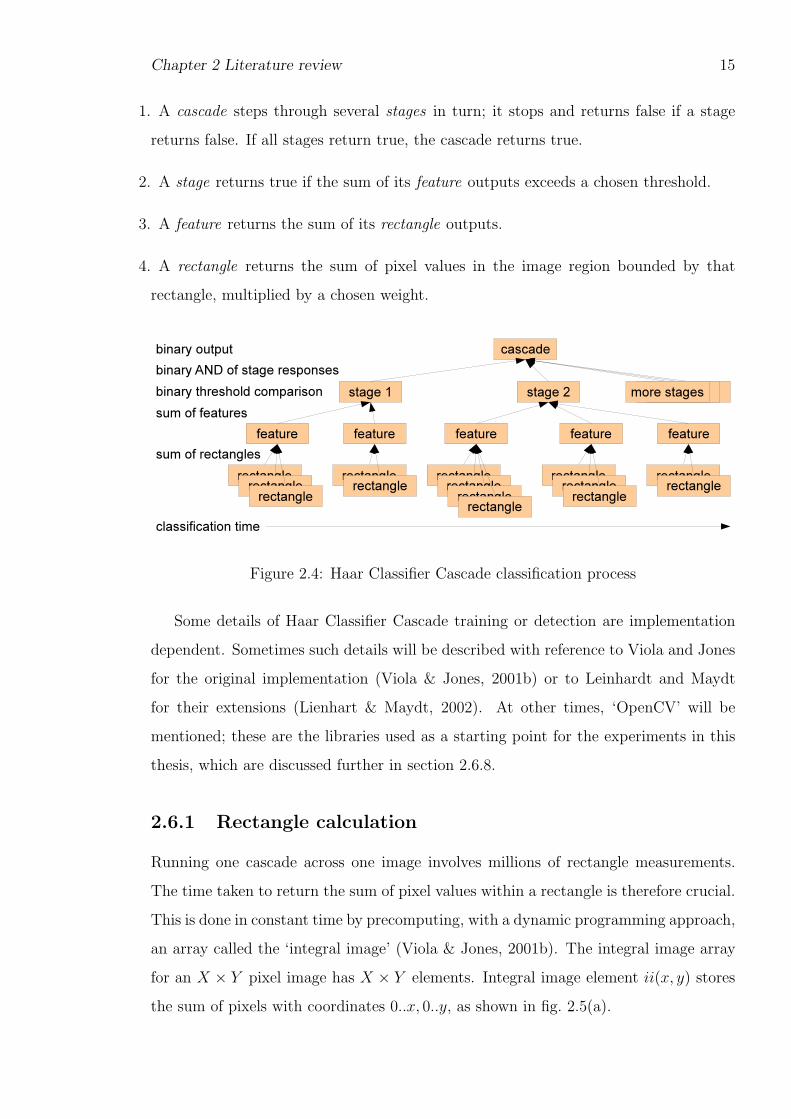
an array called the ‘integral image’ (Viola & Jones, 2001b). The integral image array

for an X ! Y pixel image has X ! Y elements. Integral image element ii(x, y) stores

the sum of pixels with coordinates 0..x, 0..y, as shown in fig. 2.5(a).


Given an existing image array I storing pixel intensity values, each element in the

integral image array ii can be calculated once the elements up and to its left are known:

ii(x, y) = ii(x, y " 1) + ii(x" 1, y) + I(x, y)" ii(x" 1, y " 1)

where

ii("1, y) = ii(x,"1) = 0

The integral image array can therefore be built in a single pass across all pixels,

taking O(X ! Y ) time. Once built, the sum of pixel values in any rectangle can

be calculated with only four array reference operations. In the example shown in

fig. 2.5(b), the sum of pixel values within the shaded rectangle is

ii(x, y) + ii(x + w, y + h)" ii(x, y + h)" ii(x + w, y)

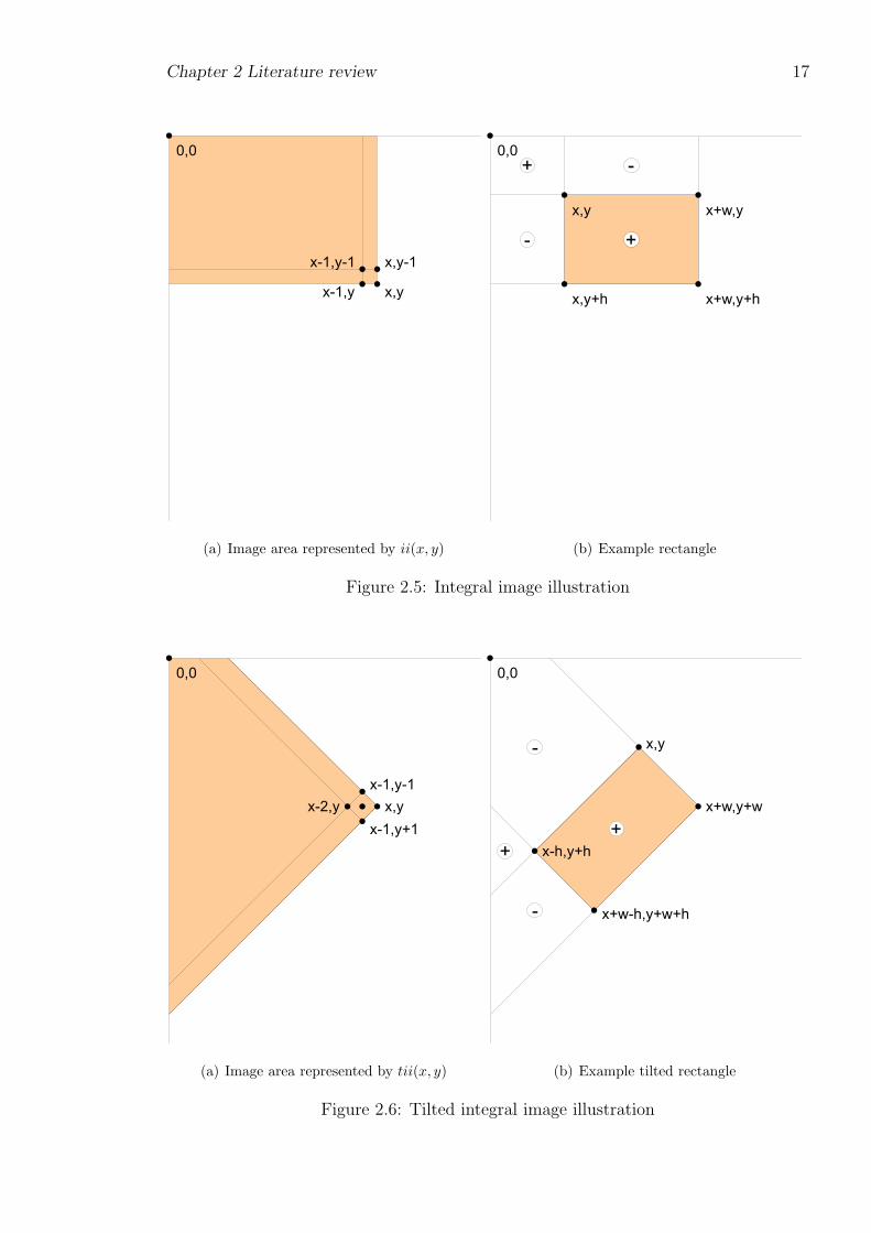
There is a limitation with the integral image described above because the rectangle

edges must be parallel with the image edges. Lienhart and Maydt added the ability

to use 45! tilted rectangles by using a tilted integral image (Lienhart & Maydt, 2002).

The tilted integral image tii must be calculated in two passes. The first pass runs from

left to right and top to bottom (x increasing, y increasing):

tii(x, y) = tii(x" 1, y " 1) + tii(x" 1, y) + I(x, y)" tii(x" 2, y " 1)

where

tii("1, y) = tii("2, y) = tii(x,"1) = 0

The second pass runs from right to left and bottom to top (x decreasing, y decreas-

ing):

tii(x, y) = tii(x, y) + tii(x" 1, y + 1)" tii(x" 2, y)

Once the tilted integral image is known, the pixel sum of any 45! tilted rectangle

can also be calculated with four array references. In fig. 2.6(b), the sum of the pixel

values within the shaded rectangle is

tii(x + w, y + w) + tii(x" h, y + h)" tii(x, y)" tii(x + w " h, y + w + h)


(a) Image area represented by ii(x, y) (b) Example rectangle

Figure 2.5: Integral image illustration

(a) Image area represented by tii(x, y) (b) Example tilted rectangle

Figure 2.6: Tilted integral image illustration


2.6.2 Features

The rectangles in section 2.6.1 may be combined to create features which compare

the intensities of di!erent image rectangles. The Haar Classifier Cascade classification

process can evaluate such features containing any combination of rectangles. However,

the training process cannot a!ord to consider every possible feature: for an x! y pixel

image region, there are x(x+1)2 ! y(y+1)

2 possible rectangles, and therefore, if repeated

rectangles are ignored, (x(x+1)2 ! y(y+1)

2 )r features containing r rectangles. A 20 ! 20

pixel cascade using 3 90!-aligned rectangles per feature therefore has approximately

8 ! 1013 features to choose from. If the tilted features are added this becomes even

more time-consuming.

Instead, the training process chooses from a limited feature set which looks for

adjacent patterns of light and dark (fig. 2.7). The first 8 features shown are of the type

used by Viola and Jones (Viola & Jones, 2001b); the 7 tilted features are only possible

with Lienhart and Maydt’s extensions (Lienhart & Maydt, 2002). The feature names

are those assigned by the OpenCV cascade training program. The feature ‘haar x2 y2’

was disabled for training in this thesis, for reasons given in section 5.1.

These features may be used at any position or scale, and may be scaled separately

on each axis. The possible positions or scales are limited by the ‘window size’ of the

cascade; Viola and Jones used a coordinate system of 24 ! 24 units for their face

detector, which meant feature selection from over 180,000 possible features (Viola &

Jones, 2001b). Lienhart et al tried window sizes of both 24!24 and 20!20 units; they

found that the smaller cascade was usually more accurate (Lienhart et al., 2003a).

Kolsch and Turk tried going beyond adjacent rectangular features by creating fea-

tures of two light and two dark rectangles, then permitting each to move freely during

training. They were able to train more accurate hand detection cascades by doing so

(Kolsch & Turk, 2004b).

The Haar Classifier Cascade feature set was inspired by the ‘2-dimensional Haar

Wavelets’ used by Oren et al. for pedestrian detection (Oren et al., 1997). This was

expanded into a generic object detection training framework (Papageorgiou et al., 1998;

Papageorgiou & Poggio, 2000). However, its feature set is smaller: it has only three

types of feature (fig. 2.8) and they are always square. Prior to Oren et al.’s work, Haar

Wavelets had also been used in image retrieval (Jacobs et al., 1995).


Figure 2.7: Haar Classifier Cascade features (Viola & Jones, 2001b; Lienhart & Maydt,

2002)

Figure 2.8: Haar Wavelet features (Papageorgiou et al., 1998)

(a) Feature 1 (b) Feature 2 (c) Feature 3 (d) All features

Figure 2.9: Example face with features from stage 1 of a face detection cascade


Fig. 2.9 shows features from the first stage of haarcascade frontalface alt2, one of

the OpenCV face detection cascades. These features represent shades within the face.

Oren, Papageorgiou et al. observed that their face detector found similar features (Pa-

pageorgiou et al., 1998)., while their pedestrian detection cascade found the pedestrian

boundary (Oren et al., 1997). Viola and Jones’ face detector also used features within

the face (Viola & Jones, 2001b), but when Kruppa et al. tried passing the entire head

and shoulders to the same training process it chose some boundary features and was

more accurate for having done so (Kruppa et al., 2003).

2.6.3 Stage training samples

Most object detection training sets contain hundreds or thousands of positive samples

– images of the object to detect. Rowley et al. had almost 1,050 faces (Rowley et al.,

1998a), while Viola and Jones used 4,916 (Viola & Jones, 2002) and Lienhart et al.

created 5,000 samples by randomly rotating and scaling 1,000 faces (Lienhart et al.,

2003a). With these numbers it is feasible to use every positive sample in training every

stage of the cascade.

Negative sample selection is a harder problem. Ideally, the negative samples would

include every possible object that is not a training positive, which is computationally

infeasible. Instead, a set of large images containing no detection objects is provided.

At each stage, these are searched for regions that are (incorrectly) classified positive by

the existing stages. These regions are then used as the negative training samples for

the next stage. Viola and Jones used 9,500 negative images, containing approximately

3.5 ! 106 possible negative regions. For each new stage 10,000 negative samples were

found within these images (Viola & Jones, 2002). Lienhart et al. similarly selected

3,000 negative samples per stage (Lienhart et al., 2003a).

2.6.4 Cascade stage boosting

Within each stage, the Haar Classifier Cascade training process boosts the training

instance weights using AdaBoost (Freund & Schapire, 1996); modifications to it have

also been tested with success (Lienhart et al., 2003a; Li & Zhang, 2004; Hou et al.,

2006). While individual stages are boosted, weights cannot be transferred between

stages because new negative training images are found for each new stage.


Stage training starts with each of the thousands or millions of possible features

described in section 2.6.2 being tested on the stage training samples. The feature that

best separates positive from negative training samples is added to the stage, and the

training instance weights are boosted. This continues, with new features being greedily

selected and added to the stage, until the stage has a set number of features, or until

the stage error rates on its positive and negative training samples fall below a chosen

threshold.

Viola and Jones used the former method, interactively choosing a number of features

per stage which led to significant error reduction for each stage (Viola & Jones, 2002).

The resulting face detection cascade had 2-, 5-, 20-, 20-, 20-, 50-, 50-, 100-, 100-, 100-,

100- and 100-feature stages, followed by twenty 200-feature stages. They also measured

the accuracy of the individual features and noted that ‘Features which are selected in

early rounds of the boosting process had error rates between 0.1 and 0.3. Features

selected in later rounds, as the task becomes more di"cult, yield error rates between

0.4 and 0.5’ (Viola & Jones, 2001b).

Lienhart and Maydt did not limit the number of features per stage, but did set

error rate thresholds. They chose di!erent positive and negative thresholds, as false

negatives in object detection are usually far more costly than false positives, and in a

Haar Classifier Cascade a single negative stage response will make the whole cascade

return negative. Because of this, they specified maximum error rates of 0.002 for

positive samples misclassified as negative and 0.5 for negative samples misclassified as

positive (Lienhart & Maydt, 2002). If stages make independent errors (possible but

not guaranteed, since their negative samples are independent but their positive samples

are identical), an n stage cascade will have a false negative rate of 1" (1" 0.002)n and

a false positive rate of 0.5n.

2.6.5 Region testing

Once built, the cascade may be used to test images. Haar Classifier Cascades run on

image regions, and return true if the image region represents the object; to determine

if an image contains the object, the cascade must be run over the images at many

di!erent locations and scales. Under the OpenCV implementation, scales start at 1.0

(the region size in pixels matches the size of the cascade) and is multiplied by 1.2 until


the region size exceeds the image size. Meanwhile, the positions tested start in the top

left corner and test points across in the image in steps of max(2.0, scale); the actual

point tested each time is rounded to the nearest pixel. If a 20 ! 20 unit detection

cascade tests a 640 ! 480 pixel image, it will evaluate 533,126 separate regions, as

listed in table 2.3. Viola and Jones used a starting scale of 1.25, a scale multiplier of

1.25 and steps of scale pixels (Viola & Jones, 2001b).

The time taken to test an image is determined by this count and by how many

stages evaluate each region. Ideally, most image regions will be obvious true negatives

and therefore be rejected by early stages of the cascade. Viola and Jones also report

that the majority of image regions were rejected by the first or second stage of their

face detector (Viola & Jones, 2001b).

Table 2.3: Counts of regions tested within a 640! 480 pixel image by a 20 ! 20 unit

cascade under OpenCV defaults


2.6.6 Merging neighbouring detections

The region testing described in section 2.6.5 results in many overlapping detections of

the same object, such as the face detections in fig. 2.10(a). These overlapping detec-

tions are partitioned into sets; Viola and Jones put any two detections with overlapping

bounds into the same set (Viola & Jones, 2001b). OpenCV uses a more complex mea-

surement: detections D and E become part of the same set if Dx " 15Dwidth # Ex #

Dx + 15Dwidth, Dy " 1

5Dwidth # Ey # Dy + 15Dwidth and 5

6Dwidth # Ewidth # 65Dwidth.

Sets of detections become a single detection with the mean coordinates of the set mem-

bers; fig. 2.10(b) shows such mean detections. The number of neighbouring detections

merged into each set is recorded; this is the number shown within each rectangle in the

example image. This neighbour count provides an approximate confidence measure-

ment: many detections around a given image region increase the likelihood that the

image region is the object the cascade is trained to detect. After merging, detections

within a larger detection with more neighbours are erased.

(a) Original detections (b) Detections after merging (numbers are the

number of neighbours merged into each detection)

Figure 2.10: Face detections before and after merging neighbouring detections

2.6.7 Rotated objects

The region testing in section 2.6.4 will still only detect objects with similar orientations

to the objects used in cascade training. This is not a problem for face detection, as

faces in most images are consistently oriented. However, it is a problem for the fish

detection considered in this thesis, as noted in section 2.4.1.1.


Jones and Viola observed that ‘a classifier trained on all poses appears to be hope-

lessly inaccurate’ but were able to detect faces at multiple orientations by combining

the output of 12 cascades, each trained on faces with di!erent orientation (Jones &

Viola, 2003a). Each cascade was trained on faces fixed around an in-plane orientation

of 0! to 330!, and randomly perturbed over a range of 30! (±15!). They also trained a

decision tree to select the best orientation for each possible image region, making their

multiple orientation classifier faster but less accurate. Kolsch and Turk investigated

this as a method for hand detection (Kolsch & Turk, 2004a); they found that ‘only

about 15! of rotations can be e"ciently detected with one detector, di!erent from the

method’s performance on faces’ and ‘More importantly, the training data must contain

rotated example images within these rotation limits’.

Similar success on rotated face detection was found with a pair of neural networks

(Rowley et al., 1998b). Given an image region, the first network returned the best

orientation for face detection on that region; it was then rotated to that orientation

and passed to an upright face detection network. The second network was trained on

faces covering a range of 20! (up to 10! away from the vertical) and was shown in tests

to successfully detect faces within the same range.

Messom and Barczak o!er the alternative of training a single cascade and rotating

it to the nearest orientation it can operate at. These would be widely separated with

only 0! and 45! integral images, so they defined 26.5! and 63.5! integral image arrays.

They report that the rotated cascades ‘provided accurate classification, although not as

good as the original vertically and horizontally aligned classifier’ (Messom & Barczak,

2006).

2.6.8 Implementation

Lienhart et al.’s implementation of Haar Classifier Cascade training and testing (Lien-

hart & Maydt, 2002; Lienhart et al., 2003a; Lienhart et al., 2003b) was used as a

starting point for the object detection routines in the Open Computer Vision libraries

(OpenCV), a collection of standard computer vision algorithms (Intel, 2006). The cas-

cade learning in chapter 5 and the detection experiments in chapters 5, 6 and 7 were

all run in OpenCV.


2.6.9 Extensions

Apart from the changes to permit rotated object detection discussed in section 2.6.7,

many other modifications to Haar Classifier Cascade training and testing have been

proposed and tested by various researchers. These include training trees instead of

cascades (Lienhart et al., 2003b), domain-specific boosting adjustments (Xiao et al.,

2003; Li & Zhang, 2004), adjusting the stage thresholds after training to improve the

performance of the complete cascade (Brubaker et al., 2005; Luo, 2005) and use of

motion-based features (Viola et al., 2005).

2.7 Classifier evaluation

New classifier learning algorithms are usually evaluated by testing against existing

classifier learners. Ideally, this is done by using each algorithm to train classifiers on

some data from a problem, then testing the performance of the classifiers on other

data from the same problem. It is very important to use separate training and testing

datasets for fair evaluation; otherwise overfitting will be rewarded. A simple option is

to randomly divide the available data into equal-sized training and testing sets. This

can cause di"culties if the available dataset is small, or contains only a few examples

of each class. These di"culties may be reduced by cross-validation.

2.7.1 Cross-validation

Instead of dividing the available data into one training set and one testing set, it is

possible to divide it in half, then train a classifier on each half and test its accuracy

on the other half. This means that every instance is used in both training and testing.

Division in half would be 2-fold cross-validation, but it is also possible to run n-fold

cross-validation, with n"1n instances in each training set and the other 1

n instances in

each testing set. A common choice for n is 10 (Witten & Frank, 2005a), although

it may be increased up to the number of instances, where it becomes leave-one-out

cross-validation. A downside of cross-validation is that training time is multiplied by

n. Within this thesis it is therefore used for classifier learning experiments on small

datasets in chapter 3, but not on the object detection cascades trained in chapter 5,

where each cascade took many hours and sometimes days to train.


2.7.2 Matching detected objects to annotated objects

For most classifier learning tasks, it is possible to compare the predicted class with

the actual class to measure accuracy. For object detection, however, the classifier will

usually report multiple positives close to the objects as mentioned in section 2.6.6.

After merging, detections such as those in fig. 2.10(b) probably still don’t exactly

match image annotations such as those in fig. 4.2. Therefore, the evaluation process

must match detections to similarly-placed annotations. Under OpenCV defaults, a

w!h pixel annotation or detection region is considered to have a size of!

w2+h2

2 units.

An annotation A is then considered to be found by a detection D if D is centred within

3#Asize10 pixels of A and 2

3Asize < Dsize < 32Asize.

2.7.3 ROC curves

Measuring accuracy alone is only appropriate if correct classification is equally impor-

tant for all classes, and incorrect misclassifications from all classes are equally bad.

This is not the case for object detection, where a detector must pass over thousands of

negative image regions for each true positive. For most problems, an algorithm could

return false for every region and achieve accuracies in excess of 99%. It is possible to set

some threshold for most object detection algorithms and count the true positives and

false positives for that threshold, but this only provides one data point. It also raises

di"culties when comparing di!erent algorithms, as noted in (Viola & Jones, 2001b).

The best way to evaluate an object detection algorithm that supports some varying

threshold is to measure its true positives and false positives at di!erent thresholds, then

plot the true positive rate against the false positive rate in order to build a Receiver

Operating Characteristic (ROC) curve (Witten & Frank, 2005c).

ROC curves may be quantitatively compared by measuring the area under the

curve, where the X axis represents the false positive rate. This is not an option for

object detection, since the potential maximum for false positives depends on the imple-

mentation. Because of this, the X axes of most object detection ROC curves show the

false positive count, not the false positive rate, and rely on visual comparisons against

other ROC curves generated on the same images (Viola & Jones, 2001a; Viola & Jones,

2001b; Jones & Viola, 2003a).


A good ROC curve will tend towards the upper left corner of the graph; any curve

that reaches it represents a 100% true positive rate for 0 false positives – ideal but

very rarely seen. In the example ROC curves shown in fig. 2.11(a), algorithm A is

consistently better than algorithms B and C: for any fixed number of false positives,

it finds more true positives, and for any fixed proportion of true positives it su!ers

fewer false positives. If algorithm B or C must be used, the choice depends on the

number of tolerable false positives or the proportion of required true positives. If false

positives are costly but not all possible true positives must be found, algorithm B is

better than C. This may be seen at the left edge of the curve, where true positives and

false positives are both low and the algorithm B line is higher. However, if a high true

positive rate is required, even at the expense of false positives, algorithm C is better

than B.

ROC curves can be built from Haar Classifier Cascade performance by imposing a

threshold on the neighbour counts described in section 2.6.6. The first and rightmost

point on the curve is the true positive/false positive counts for the cascade’s detections

before merging. The second point on the curve is for the regions found by merging

at least two neighbours. This continues, with the nth point on the curve showing the

performance for detections merged from at least n neighbours. As n increases, both true

positives and false positives decrease, so the points move left and down. Eventually,

n becomes infinite and no detections are considered, leading to 0 true positives and

0 false positives. An ROC curve created from such face detection cascade testing is

shown in fig. 2.11(b).

Similar graphs may plot false negatives on the Y-axis instead of true positives,

flipping the graph about the Y-axis, as in (Lienhart & Maydt, 2002). Precision-

recall curves, which show a plot of precision"

True positivesTrue positives+False positives

#against recall

"True positives

True positives+False negatives

#have similar shapes (Sahami et al., 1998).

Some classifiers may only yield a small number of detections even at their most

permissive, creating ROC curves that don’t completely extend to the right-hand Y-

axis. This is normal; the decision of the maximum number of false positives to plot

is arbitrary. The ROC curves in this thesis have their maximum false positives set

approximately equal to the potential maximum true positives.


0

50

100

150

200

250

300

350

400

0 100 200 300 400False positives

Tru

e p

os

itiv

es

0

0.2

0.4

0.6

0.8

1

Tru

e p

os

itiv

e r

ate

A

B

C

(a) Example ROC curves

0

100

200

300

400

500

0 100 200 300 400 500False positives

Tru

e p

os

itiv

es

0

0.2

0.4

0.6

0.8

1

Tru

e p

os

itiv

e r

ate

2 neighbours

3 neighbours

12 neighbours

31 neighbours

4 neighbours

(b) Example face detection ROC curve

Figure 2.11: Example Receiver Operating Characteristic (ROC) curves

2.7.3.1 Combining ROC curves

Many comparisons between object detection methods in this test involve whole sets of

cascades. To compare methods, these steps are followed:

1. ROC curves are constructed for every cascade.

2. All points are extracted from every ROC curve.

3. Every point for which another point exists with equal or more true positives and less

than or equal false positives is discarded.

4. A curve is plotted starting from 0,0 and passing through the remaining points, ordered

by ascending true positive count.

The individual points and resulting ‘best’ curve for a detection method are plotted in

fig. 2.12.


0

100

200

300

400

500

0 200 400 600 800

False positives

Tru

e p

os

itiv

es

0

0.2

0.4

0.6

0.8

1

Tru

e p

os

itiv

e r

ate

Range=0° Range=25°Range=5° Range=30°Range=10° Range=45°Range=15° Range=60°Range=20° Range=90°

Best curve

Figure 2.12: Example of combining points from multiple ROC curves to create a single

‘best’ ROC curve

2.8 Conclusions

This chapter has described existing research in classifier learning and object detection,

with emphasis upon Haar Classifier Cascades for rotated object detection. The follow-

ing chapters will attempt to extend on it by creating algorithms which are either faster

or more accurate than the ones described here. They will also thoroughly compare

di!erent options for rotated object detection and consider issues specific to seahorse

detection – a previously unstudied problem in marine creature detection.

Date post:	03-Sep-2018
Category:	Documents
Upload:	lymien
View:	217 times
Download:	0 times

2 Literature review - Open Access Repository · 2 Literature review This chapter discusses the...

Documents