20 Water transmission Nemanja Trifunovic · 20 Water transmission Nemanja Trifunovic. ... needed to...

20 Water transmission

Nemanja Trifunovic

http://www.a-pdf.com/?product-split-demo

Water transmission

20.1 Introduction

Water transmission frequently forms part of small community water supply systems; in

that respect they do not differ from large schemes. The water needs to be transported

from the source to the treatment plant, if there is one, and onward to the area of dis-

tribution. Depending on the topography and local conditions the water may be conveyed

through free-flow conduits (figure 20.1), closed conduits (figure 20.2) or a combination of

both (figure 20.3). The water conveyance will be either under gravity or by pumping.

Free-flow conduits are generally laid at a uniform slope that closely follows the hydraulic

grade line1. Examples of such conduits are canals, aqueducts, tunnels or partially filled

pipes. If a pipe or tunnel is completely full, the hydraulic gradient and not the slope of

the conduit will govern the flow. The hydraulic laws of closed conduit flows, also

commonly called pressurised flows, apply in this case. Pressurised pipelines can be laid

up- and downhill as needed, as long as they remain at sufficient distance below the

hydraulic grade line, i.e. a certain minimum pressure is maintained in the pipe.

Free-flow conduits have a limited application in water supply practice in view of the

danger that the water will get contaminated. They are never appropriate for the

conveyance of treated water, but may well be used for transmission of raw water.

For community water supply purposes, pressurised pipelines are the most common

means of water transmission. Whether for free flow or under pressure, water

transmission conduits generally require a considerable capital investment. A careful

consideration of all technical options and their costs and discussion with the community

groups that will support and manage the system are therefore necessary when selecting

the best solution in a particular case.

Routes always need to be checked with community members as well to make use of

local knowledge and ensure cultural acceptability (technically desirable routes may, for

example, run through a burial site or be unacceptable for other local reasons).

442

20

1 Its altitude and the water pressure in it define the piezometric head of each flow cross-section. The hydraulic

grade line connects elevations of the piezometric heads and represents the potential energy of the flow. The

slope of the hydraulic grade line is called the hydraulic gradient. For free-flow conduits it is the slope of the

water surface. For closed conduits the hydraulic grade line slopes according to the head loss.

IRC_SCWS-book 27 gtb 20-11-2002 14:58 Pagina 442

443

Chapter 20

Fig. 20.1. Free-flow conduit

Fig. 20.2. Closed conduit

Fig. 20.3. Combined free-flow/closed conduit


20.2 Types of water conduits

Canals

Canals are laid in areas where the required slope of the conduit more or less coincides

with the slope of the terrain. Generally they have a trapezoidal cross-section but the

rectangular form will be more economical when the canal traverses solid rock. Flow

conditions are assumed to be uniform if a canal has the same cross-section dimensions,

slope and surface lining throughout its length.

Aqueducts and tunnels

Aqueducts and tunnels are constructed in hilly areas. They should be of such a size that

they are approximately three-quarters full at the design flow rate. Tunnels for free-flow

water transmission are frequently horseshoe shaped. They are constructed to shorten the

overall length of a water transmission route, and to circumvent the need for any conduits

traversing uneven terrain. To reduce head losses and infiltration seepage, tunnels are

usually lined. However, when constructed in stable rock they require no lining.

Free-flow pipelines

Free-flow pipelines are used for transport of smaller quantities of water than tunnels.

Compared with canals and aqueducts they offer better protection from pollution. Due

to the free-flow conditions, simple materials may be used for construction. Glazed clay

or concrete pipes should be adequate. Similar hydraulic conditions occur as for other

free-flow conduits.

Pressurised pipelines

The routing of pressurised pipelines is much less limited by the topography of the area

to be traversed, than is the case of canals, aqueducts or free-flow pipelines. A pressure

pipeline may run up- and downhill and there is considerable freedom in selecting the

pipeline alignment. Nevertheless, such pipelines often follow the topography quite

closely, being buried at a similar depth for the length of the route. Also, a routing

alongside roads or public ways will be preferred in order to facilitate inspection (for

detection of any damage, leakage at pipe joints, faulty valves, etc.) and to provide ready

access for maintenance and repair.

20.3 Design parameters

Design flow

The water demand in a distribution area will fluctuate considerably during a day. Usually

a service reservoir is provided to accumulate and even out the variation in water

demand. The service reservoir is supplied from the transmission main, and is located at

a suitable position to be able to supply the distribution system (Fig. 20.4). Again, its site

444


needs to be chosen by the local people, based on technical advice and their own socio-

cultural criteria. The transmission main is normally designed for the carrying capacity

needed to supply water demand on the maximum consumption day at a constant rate.

All hourly variations in the water demand during the day of maximum consumption are

then assumed to be evened out by the service reservoir.

The number of hours the transmission main operates each day is another important

factor. For a water supply with diesel engine or electric motor-driven pumps, the daily

pumping often is limited to 16 hours or less. In such a case, the design flow rate for the

transmission main as well as the volume of the service reservoir need to be adjusted

accordingly.

445

Chapter 20

Fig. 20.4. Transmission main and service reservoir (schematic)

Design pressure

Pressure as a design parameter is only relevant for pressurised pipelines. Consumer

connections on transmission lines are rare, so the water pressure can be kept low,

provided that the hydraulic grade line is positioned above the pipe over its entire length

and for all flow rates. A minimum of a few metres water column is also required to

prevent intrusion of pollution through damaged parts of the pipe or faulty joints. In fact,

nowhere should the operating pressure in the pipeline be less than 4-5 mwc (metres

water column).


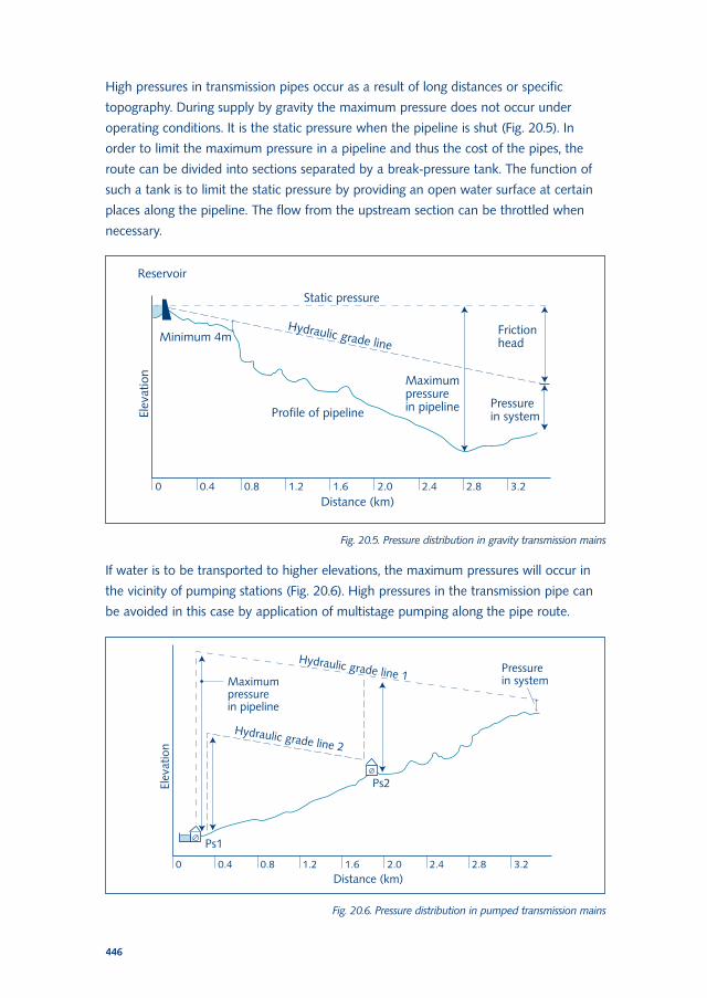
High pressures in transmission pipes occur as a result of long distances or specific

topography. During supply by gravity the maximum pressure does not occur under

operating conditions. It is the static pressure when the pipeline is shut (Fig. 20.5). In

order to limit the maximum pressure in a pipeline and thus the cost of the pipes, the

route can be divided into sections separated by a break-pressure tank. The function of

such a tank is to limit the static pressure by providing an open water surface at certain

places along the pipeline. The flow from the upstream section can be throttled when

necessary.

446

Fig. 20.5. Pressure distribution in gravity transmission mains

If water is to be transported to higher elevations, the maximum pressures will occur in

the vicinity of pumping stations (Fig. 20.6). High pressures in the transmission pipe can

be avoided in this case by application of multistage pumping along the pipe route.

Fig. 20.6. Pressure distribution in pumped transmission mains


Critical pressures may also develop as a result of pressure surge or water hammer in the

pipeline. This phenomenon is caused by the instant or too rapid closure of valves, or by

sudden pump starts or stops, e.g. due to electricity failure. A longitudinal water wave

created in such a way causes over- and under-pressures well above the normal working

pressure. This is potentially a very dangerous situation that may result in damage to the

pipeline over long distances. Proper prevention includes construction of surge tanks, air

vessels or water towers as well as selection of suitable pipe materials that can withstand

the highest pressures. Regarding valves, specified minimum shut-off times should be

strictly respected. This makes it important how communities choose, train and supervise

valve operators and that operators understand, and practise, the proper regulation of

the valves.

Design velocity and hydraulic gradient

A velocity range is established for design purposes for two reasons. On the one hand,

a certain minimum velocity will be required to prevent water stagnation causing

sedimentation and bacteriological growth in the conduits. On the other hand, the

maximum velocity will have to be respected in order to control head losses in the

system as well as to reduce the effects of water hammer.

The velocity of flows in canals, aqueducts and tunnels usually ranges between 0.4 and

1.0 m/s for unlined conduits, and up to 2 m/s for lined conduits. Flows in pressurised

transmission mains have the velocity range between 1 and 2 m/s.

In the case of pressurised pipes, design values may also be set for the hydraulic gradient.

This is done primarily to limit the head losses, i.e. to minimise the energy consumption

for pumping the water. Common values of the hydraulic gradients for transmission pipes

are around 0.005, which means 5 mwc of head loss per km of the pipe length.

20.4 Hydraulic design

Flow Q (m3/s) through a cross-section A (m2) is determined as Q = vA, where v (m/s) is

the mean velocity of the cross-section. Assumptions of ‘steady’ and ‘uniform’ flow apply

in basic hydraulic calculations for the design of water transmission systems. The flow is

steady if the mean velocity of one cross-section remains constant within a certain period

of time. If the mean velocity between the two cross-sections is constant at a certain

moment, the flow is uniform.

447

Chapter 20


Free-flow conduits

The Strickler formula is widely used for conduits with free-flow conditions. The formula

reads:

448

where:

v = mean water velocity in the cross-section (m/s)

Ks = Strickler coefficient (m1/3/s)

R = hydraulic radius (m)

S = hydraulic gradient (m/km)

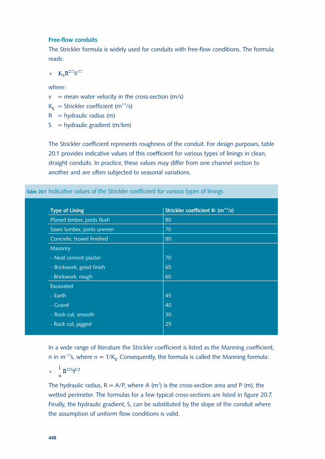
The Strickler coefficient represents roughness of the conduit. For design purposes, table

20.1 provides indicative values of this coefficient for various types of linings in clean,

straight conduits. In practice, these values may differ from one channel section to

another and are often subjected to seasonal variations.

Table 20.1 Indicative values of the Strickler coefficient for various types of linings

Type of Lining Strickler coefficient Ks (m1/3/s)

Planed timber, joints flush

Sawn lumber, joints uneven

Concrete, trowel finished

Masonry

- Neat cement plaster

- Brickwork, good finish

- Brickwork, rough

Excavated

- Earth

- Gravel

- Rock cut, smooth

- Rock cut, jagged

80

70

80

70

65

60

45

40

30

25

In a wide range of literature the Strickler coefficient is listed as the Manning coefficient,

n in m-1/3s, where n = 1/Ks. Consequently, the formula is called the Manning formula:

The hydraulic radius, R = A/P, where A (m2) is the cross-section area and P (m), the

wetted perimeter. The formulas for a few typical cross-sections are listed in figure 20.7.

Finally, the hydraulic gradient, S, can be substituted by the slope of the conduit where

the assumption of uniform flow conditions is valid.


Closed Conduits

The Strickler and Manning formulas are also applicable for closed conduits by

introducing the real hydraulic gradient of the flow and the wetted perimeter as the full

perimeter of the conduit. Nevertheless, a problem may occur in the selection of the

roughness factors for a wide range of pipe materials and flow conditions.

More appropriate formulas for computing the head loss of water flowing through

a pressurised pipeline are those of Darcy-Weisbach and Hazen-Williams.

The Darcy-Weisbach formula states:

449

Chapter 20

Fig. 20.7. Geometric properties of typical cross-sections

where:

DH = head loss (mwc)

L = pipe length (m)

D = pipe diameter (m)

l = friction factor (-)

v = the mean velocity in the pipe (m/s)

g = gravity (9.81 m/s2)

Q = flow rate (m3/s)


Introducing the hydraulic gradient, S = DH/L, the formula can be rewritten as:

450

The factor l is the friction coefficient that can be calculated by the Colebrook-White

formula:

where:

Re = the Reynolds number (-)

k = absolute roughness of the inner pipe wall (mm)

D = pipe diameter (mm)

The Reynolds number indicates the flow regime:

where:

v = the mean velocity in the pipe (m/s)

D = pipe diameter (m)

= kinematic viscosity (m2/s)

Finally, the kinematic viscosity is dependent on the water temperature. For T in °C:

The Colebrook-White formula is developed for a turbulent flow regime, i.e. Re-values

above ± 4000. The common values in practice are much higher, typically in the order of

104 and 105. If by chance the flow is laminar (Re < 2000), the friction factor l will be

calculated as: l = 64/Re.

Calculation by the Colebrook-White formula is not straightforward, as the l-factor appears

on both sides of the equation. The alternative formula of Barr can be used instead:

To by-pass somewhat cumbersome computations, the work can also be facilitated by use

of the Moody diagram, hydraulic tables or pipe charts (see Chadwick & Morfett, 1996 or

Bhave, 1991). These tables/charts, which are produced for certain water temperatures


and k-values, show the velocities (flows) for a range of pipe diameters and hydraulic

gradients. Any of the three parameters can be determined by fixing the other two.

The common range of k-values is listed in table 20.2 for various pipe materials. For

practical calculation these values can be increased depending on the number of years the

pipe was in service and the influence of head losses caused by bends, joints, valves, etc.

451

Chapter 20

Table 20.2 Absolute roughness (Bhave, 1991)

Pipe material k (mm)

Asbestos cement

Bitumen/Cement lined

Wrought iron

Galvanised/Coated cast iron

Uncoated cast iron

Ductile iron

Uncoated steel

Coated steel

Concrete

Plastic, PVC, PE

Glass fibre

Brass, cooper, lead

0.015 - 0.03

0.03

0.03 - 0.15

0.06 - 0.3

0.15 - 0.6

0.03 - 0.06

0.015 - 0.06

0.03 - 0.15

0.06 - 1.5

0.02 - 0.05

0.06

0.003

The Hazen-Williams formula is simpler, although less accurate than the Darcy-Weisbach

equation. It states for SI-units:

The values of the Hazen-Williams factor, Chw, are listed in table 20.3.

This formula is applicable for a common range of flows and diameters. Its accuracy

becomes reduced at lower values of Chw (much below 100), and/or velocities that are

appreciably lower or higher than 1 m/s. Also, the Hazen-Williams formula is not

dimensionally uniform and if other units are used than SI, it has to be readjusted.

Nevertheless, due to its simplicity this formula is still widely used in the USA and in

many, predominantly Anglophone, developing countries.


Application of the discussed head loss formulas is illustrated in the examples.

Example 1

Determine the capacity of the rectangular concrete canal if the water depth is 0.2 m.

The width of the canal is 1.0 m and the slope of the bottom is S = 10/00.

Solution

From table 20.2, Ks for concrete = 80 m1/3/s. Further:

452

Table 20.3 The Hazen-Williams factors (Bhave, 1991)

Pipe material

Uncoated cast iron

Coated cast iron

Uncoated steel

Coated steel

Wrought iron

Galvanised iron

Uncoated asbestos

cement

Coated asbestos

cement

Concrete, minimum

values

Concrete, maximum

values

Prestressed concrete

PVC, brass, cooper,

lead

Wavy PVC

Bitumen/cement lined

Chw

D=75 mm

121

129

142

137

137

129

142

147

69

129

147

142

147

Chw

D=150 mm

125

133

145

142

143

133

145

149

79

133

149

145

149

Chw

D=300 mm

130

138

147

145

147

150

84

138

147

150

147

150

Chw

D=600 mm

132

140

150

148

150

152

90

140

150

152

150

152

Chw

D=1200 mm

134

141

150

148

95

141

150

153

150

153


Example 2

Find out the head loss in the concrete transmission pipe, L = 300 m and D = 150 mm,

flowing full. The flow rate is 80 m3/hour and the water temperature is 10°C. Compare

the results of the Darcy-Weisbach, Hazen-Williams and Strickler formulas.

Solution

For water temperature of 10°C, the kinematic viscosity:

The pipe velocity:

and the Reynolds number:

From table 20.3, the k-value for concrete pipes ranges between 0.06 and 1.5 mm.

For k = 0.8 mm, the l factor from the Barr equation:

Finally:

According to table 20.4, the Hazen-Williams factor for ordinary concrete pipe

D = 150 mm ranges between 79 and 133. For Chw assumed at 105:

Consequently:

Finally, for Ks = 85 m1/3/s:

All three formulas show similar results in this case. This can differ more substantially for

different choice in roughness parameters. E.g. in case of Chw = 120, the same

calculation by the Hazen-Williams formula would yield DH = 4.03 mwc while for

Ks = 80 m1/3/s, the Strickler formula gives DH = 5.90 mwc.

453

Chapter 20


In practice, the accuracy of any head loss formula is of less concern than a proper

choice of the roughness factor (k, Chw or Ks) for a given surface. Errors in results

originate far more frequently from insufficient knowledge about the condition of the

conduit, than from a wrong choice of formula.

Example 3

What will be the flow in a 100 mm-diameter pipe to transport water from a small dam

to a tank at 600 m distance? The difference between the water surfaces in the two

points is 3.60 m. The absolute roughness of the pipe wall is k = 0.25 mm and the water

temperature equals 10°C.

Solution

The difference between the water levels indicates the available head loss. Hence, DH =

3.60 mwc and S = 3.60/600 = 0.006. From the previous example, = 1.31 * 10-6 m2/s

for the water temperature of 10°C. The calculation has to be iterative due to the fact

that the velocity (flow) is not known and it influences the Reynolds number, i.e. the flow

regime. A common assumption is v = 1 m/s. Further:

The calculated velocity is different from the assumed one of 1 m/s. The procedure has

to be repeated starting with this new value. For v = 0.66 m/s, Re = 5.06 * 10-4, and

l =0.028, which yields v = 0.65 m/s. The difference of 0.01 m/s is considered as

acceptable and hence:

20.5 Water transmission by pumping

Transmission by pumping is applied in cases when the water has to be transported over

large distances and/or to higher elevations. The pumping head is the total head, and

comprises the static head plus the friction head loss for the design flow rate. The pump

to be selected must be able to provide this head (Fig. 20.9).

The head loss corresponding to the design flow rate can be computed for several pipe

diameters using the principles presented in paragraph 20.4. Each combination of the

pumping head and corresponding pipe diameter should be capable of supplying the

454


required flow rate over the required distance, and up to the service reservoir. Smaller

pipe diameters will require a higher pumping head to overcome the increase in head

losses, and the other way round. As a result, one pipe diameter will represent the least-

cost choice taking into account the initial costs (capital investment), maintenance costs

and the energy costs for pumping. The total cost, capitalised, is the basis for selecting

the most economical pipe diameter.

455

Chapter 20

Fig. 20.8. Pumped supply

For this analysis, the calculated costs for different pipe sizes are plotted in a graph of

which figure 20.9 shows an example.

Fig. 20.9. Determination of most economical pipe diameter


456

The most economical pipe diameter will tend to be large when energy costs are high,

unit costs of pipe low, and capital interest rates low. Nevertheless, it should not be

forgotten that a larger pipe means lower velocity, i.e. potential water quality problems.

As a preliminary estimate, the range of possible most economic diameters can be

selected based on velocities around 1 m/s.

Selection of pumps

Various types of pumps have been mentioned in chapter 9: centrifugal, axial-flow,

mixed-flow and reciprocating pumps. The choice of pump will generally depend on its

duty in terms of pumping head and capacity.

Pumps with rotating parts have either a horizontal or a vertical axis. The choice between

these is generally based on the pump-motor drive arrangement and the site conditions.

At a site subject to flooding, the motor and any other electrical equipment must be

placed above the flood level. Local knowledge is invaluable to identify such risks.

In water transmission for community water supply purposes it is not unusual that

a substantial head is required. This implies that the pumps selected frequently are of the

centrifugal (radial-flow) type.

Many drinking water pumps are designed to run (almost) continuously throughout

a day. In such cases an increase in pump efficiency of a few percent may represent

a considerable saving in the running costs over a long period of time. However for rural

water supplies, an even more important requirement is that any pump installed should

be reliable.

Fig. 20.10. Typical pump characteristics


The head/capacity characteristic of a pump and its efficiency are indicated in catalogues

that are supplied by the manufacturers of the pump. Figure 20.10 shows an example.

In practice it is not an easy task to have a pump permanently run at its maximum

efficiency because the operating point of the pump is determined by both the pumping

head and the capacity, and thus can vary considerably. This applies to some degree for

water transmission systems and even more in the case of distribution networks.

Efficiencies of small-capacity pumps operating under the conditions of rural areas in

developing countries are frequently quite low. A tentative estimate would be as low as

30% for a 0.4-Kilowatt pump, up to 60% for a 4-Kilowatt pump.

Power requirements

The power required for driving a pumping unit can be computed by the following formula:

457

Chapter 20

where:

N = power required for pumping (Watts)

Q = maximum pumping capacity (m3/s)

r = specific weight of water (kg/m3)

= pumping efficiency (-)

Hs = static head (m)

S = hydraulic gradient (m/km)

L = pipe length (m)

Introducing the specific weight in kg/dm3 gives the result for power in Kilowatts (kW).

Assuming r = 1 kg/dm3, g = 10 m/s2 and for small-capacity pumps estimated at 0.5

(50 %), the above formula can be further simplified to:

This formula gives N in Watts for Q in l/s, either in Kilowatts for Q in m3/s. The head is

in both cases specified in metres of water column (mwc).


Example

For a water supply, pumping is required at rate of 150,000 litres per 12 hours. The static

head is 26 m, and the length of the pipeline is 450 m. Determine the power

requirement for pumping station, if a PVC pipe, D = 80 mm is used.

Solution

458

From table 20.4, Chw for PVC of D = 80 mm can be assumed at 147. Further:

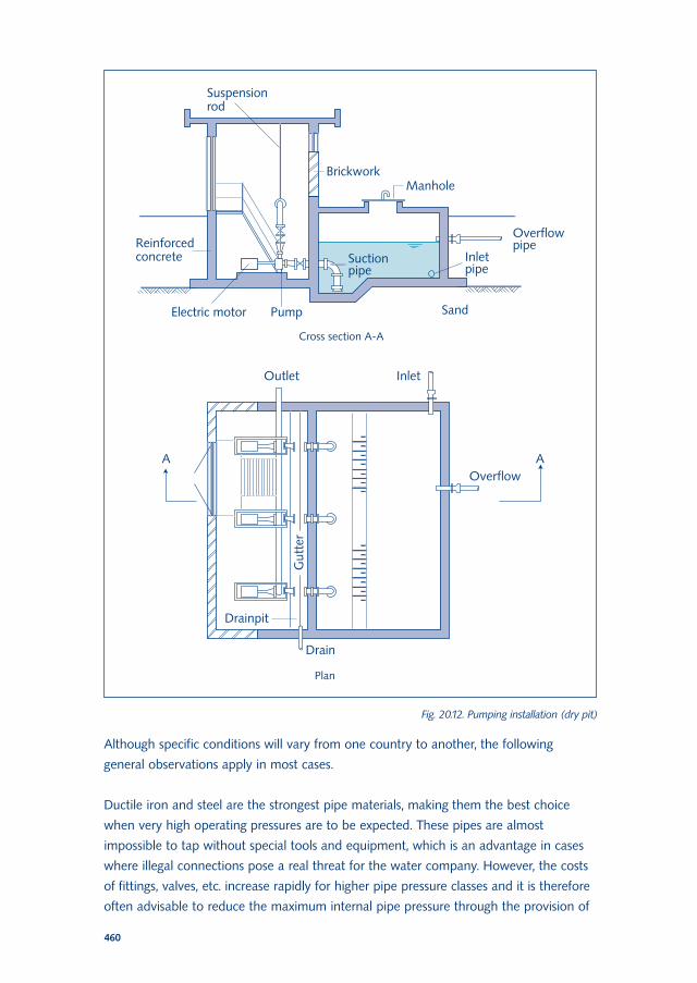
Pump Installations

Pumping stations may be of the wet-pit type (with submersible pumps or pumps driven

by motors placed above the pump in the sump), or of the dry-pit type (pump installed

in a pump room). The wet-pit type has the pumps immersed in the water, and the dry-

pit type has the pump in a dry room separated from the water by a wall.

For ease of installation horizontal pumps are sometimes situated above ground level. In

that case the pump must be of the self-priming type, which is generally not such

a reliable arrangement for rural water supply installations. With too high values of the

suction head, a risk of cavitation may occur.

Examples of various types of pump installations are shown in figures 20.11 and 20.12.

20.6 Pipe materials

Pipelines frequently represent a considerable investment and selection of the right type

of pipe is important. Pipes are available in various materials, sizes and pressure classes.

The most common materials are cast iron (CI), ductile iron (DI), steel, asbestos cement

(AC), polyvinyl chloride (PVC) and polyethylene (PE). Galvanised steel (GS) is sometimes

selected because of its resilience for situations where subsidence of the pipes is

expected. Apart from these, indigenous materials such as bamboo may have limited

application.


Factors influencing the choice of pipe material are:

• the cost and local availability of different types of pipe;

• the design pressure in the distribution system;

• the corrosiveness of the water and of the soil in which the pipes are to be laid;

• conditions such as traffic overload, proximity to sewer lines, and crowded residential

areas.

459

Chapter 20

Fig. 20.11. Pumping station with horizontal pumps (self priming)


Although specific conditions will vary from one country to another, the following

general observations apply in most cases.

Ductile iron and steel are the strongest pipe materials, making them the best choice

when very high operating pressures are to be expected. These pipes are almost

impossible to tap without special tools and equipment, which is an advantage in cases

where illegal connections pose a real threat for the water company. However, the costs

of fittings, valves, etc. increase rapidly for higher pipe pressure classes and it is therefore

often advisable to reduce the maximum internal pipe pressure through the provision of

460

Fig. 20.12. Pumping installation (dry pit)


a pressure reducing valve or break-pressure tank. A break-pressure tank is generally

more reliable than a pressure reducing valve.

In spite of higher investment costs, ductile iron pipes are a better alternative than cast

iron pipes because they have a longer service life, are lighter and more flexible and

require hardly any maintenance. The pipe is practically corrosion resistant due to

coatings applied inside and out.

Compared with metal pipes, asbestos cement pipes are light and easy to handle. Except

for soils containing sulphate, these pipes show good corrosion resistance. They are

widely used in sizes up to 300 mm, mainly for secondary pipes and for low-pressure

mains. Asbestos cement may be less suitable for transmission mains because non-

authorised tapping of such mains is possible. Moreover, this pipe material may be

subject to scale bursts when tapped without sufficient skill.

The carcinogenic effect of AC materials has been analysed carefully in recent years.

Although not dangerous when used to supply drinking water, asbestos fibres can be

very harmful when inhaled. AC pipes are slowly being phased-out due to possible

hazards during manufacturing and maintenance works. Alternative materials are in this

case PVC, PE or DI.

Polyvinyl chloride pipes have the advantage of easy jointing and their corrosion

resistance is good. They can be manufactured in several quality classes to meet the

selected design pressure. PVC, however, suffers a certain loss in strength when exposed

to sunlight for long periods of time and care should be taken to cover the pipes when

these are stocked in the open. This is one of the aspects that informed villagers can

easily check. Secondly, in case of calamity, PVC pipe breaks along considerable lengths,

causing large water losses. Therefore, the pipe should not be laid directly on rocky soil

and heavy surface loads are to be avoided. Burying the pipe deeper in the ground can

diminish the effect of extreme ambient temperatures. Non-authorised tapping of rigid

plastic (PVC) mains is also difficult to prevent.

High-density polyethylene (PE) is a very suitable pipe material for small-diameter mains

because it can be supplied in coil. The potential of laying this pipe in longer lengths

reduces the number of necessary joints. Particularly in cases where rigid pipe materials

would necessitate a considerable number of special parts such as elbows and bends, the

flexible PE makes for an ideal pipe material. Polyethylene does not deteriorate when

exposed to direct sunlight. Conventional jointing of the PE-pipes may cause leakage and

welding is considered to be a better alternative. Furthermore, formation of bio-film in

the pipe may be enhanced in some cases.

461

Chapter 20


To summarise, for pipelines of small-diameter (less than 200 mm) PVC and PE may

generally be the best alternative unless high working pressures are expected (above 60

mwc). These pipes can also be used for medium- to large-sized pipelines (diameters up

to 500-600 mm) where lower pressures can be maintained. Cast iron, ductile iron and

steel are generally only used for large-diameter mains and also in cases where very high

pressures necessitate their use in small- or mid-range diameter pipes. Due to heavy

weight and lower flexibility, CI pipes are becoming less advantageous than DI, despite

lower prices. Asbestos cement can be considered only if no other viable alternative

exists. Stringent measures that have to be introduced while handling these pipes involve

the prevention of the production and inhalation of fibre dust (use of special saws,

cutting under wet conditions, protection masks for the workers, etc).

Table 20.4 lists the comparative characteristics of pipe materials for pipelines.

Valves

Apart from the sluice (“gate”) valves and non-return valves fitted to the pump outlets in

case of a pumped supply, various types of valves and appurtenances are used in the

transmission main proper. As the pipeline will normally follow the terrain, provision must

be made for the release of trapped air at high points. Air release valves should be

provided at all these points on the pipeline and may also be required at intermediate

positions along long lengths of even gradient. To avoid under-pressure, air admission

valves may also have to be used. These serve to draw air into the pipeline when the

internal pressure falls below a certain level. At the lowest points of the pipeline, drain or

discharge valves must be installed to facilitate emptying or scouring the pipeline.

In long pipelines sluice valves should be installed to enable sections of the pipeline to be

isolated for inspection or repair purposes. Especially when parallel pipes are used it is

advantageous to connect them at intervals. In the event of leakage or pipe burst only

one section of such an interconnected main needs to be taken out of operation,

whereas the other sections and the entire other main can still be used. In this way the

capacity of the parallel pipe as such is hardly reduced. It should be mentioned that this

advantage is obtained at a cost because each connection between the twin mains

requires at least five valves.

Sluice valves perform their function either fully opened or completely closed. For pipe

diameters of 350 mm and less, a single valve may be used. For larger diameters a small-

diameter bypass with a second valve will be needed because otherwise the closing of

the large-diameter valve might prove very difficult. In those cases where the flow of

water has to be throttled by means of a valve, butterfly valves should be used. This type

of valve may equally be used instead of the sluice valves mentioned above, but the cost

is usually somewhat higher.

462


463

Chapter 20

Table 20.4 Comparison of pipe materials (Smith et al., 2000)

CI Lined DICharacteristic

Metal

Poor

Fair

Moderate

High

High

T/D*

Fair

Moderateto high

High

Moderate

Low tomoderate

Fair

NA

NA

Metal

Good

Moderate

Moderate

High

High

T/D

Good

Low

Low

High

Low tomoderate

Very good

100-250

80-1600

Steel

Metal

Poor

Poor

Moderate

High

High

T/D

Good

Moderateto high

Moderate

Moderate

Low tomoderate

Very good

Varies

100-3000

GS

Metal

Fair

Fair

Moderate

Moderate

High

T/D

Good

Moderateto high

Moderate

Moderate

Low tomoderate

Fair

NA

NA

AC

Concrete

Good

Good

Low

Moderate

Moderate

D

Fair

Low tomoderate

Low

Moderate

Moderate

Good

70-140

100-1100

PVC

Plastic

Good

Very good

Low

Low

Moderate

D

Poor

Low

Moderate

Low

Moderateto high

Good

Max.160

100-900

PE

Plastic

Good

Very good

Low

Low

Moderate

S/D

NA

Low

Low

Low

High

Poor

Max.140

100-1600

Material category

Int. corrosion resistance

Ext. corrosion resistance

Cost

Weight

Life expectancy

Primary use

Tapping characteristics

Internal roughness

Effect on water quality

Equipment needs

Ease of installation

Joint watertightness

Pressure range (mwc)

Diameter range (mm)

* T: transmission, D: distribution, S: service connections

Fig. 20.13. Various types of valves


Bibliography

Bhave, P.R. (1991). Analysis of flow in water distribution systems. Lancaster, PA, USA,

Technomic Publishing.

Chadwik, A. and Morfett, J. (1996). Hydraulics in civil and environmental engineering.

London, UK, E&FN SPON.

Dangerfield, B.J. (1983). Water supply and sanitation in developing countries. (Water

practice manuals; no. 3). London, UK, Institution of Water Engineers and Scientists

(IWES).

Fair, G.M.; Geyer, J.C.; Okun, D.A. (1966). Water and wastewater engineering. Vol. 1.

New York, NY, USA, John Wiley.

Larock, B.E.; Jeppson, R.W. and Watters, G.Z. (2000). Hydraulics of pipeline systems.

Boca Raton, FL, USA, CRC Press.

KSB (1990). Centrifugal pump design. S.l., KSB.

Smith, L.A.; Fields, K.A.; Chen, A.S.C. and Tafuri, A.N. (2000). Options for leak and break

detection and repair for drinking water systems. Columbus, OH, USA, Battelle Press.

464


Date post:	19-Mar-2020
Category:	Documents
Upload:	others
View:	2 times
Download:	1 times

20 Water transmission Nemanja Trifunovic · 20 Water transmission Nemanja Trifunovic. ... needed to...

Documents