2001- J Fluid Mechanics_ Swirling Flow of Viscoelastic Fluids. Part 1

J. Fluid Mech. (2001), vol. 429, pp. 67–115. Printed in the United Kingdom

c© 2001 Cambridge University Press

67

Swirling flow of viscoelastic fluids. Part 1.Interaction between inertia and elasticity

By J A S O N R. S T O K E S1, L A C H L A N J. W. G R A H A M2,N I C K J. L A W S O N1 AND D A V I D V. B O G E R1

1Department of Chemical Engineering, The University of Melbourne, Parkville 3052, Australia2Advanced Fluid Dynamics Laboratory, CSIRO Building Construction and Engineering,

Graham Road, Highett 3190, Australia

(Received 29 December 1998 and in revised form 11 October 1999)

A torsionally driven cavity, consisting of a fully enclosed cylinder with rotating bottomlid, is used to examine the confined swirling flow of low-viscosity Boger fluids forsituations where inertia dominates the flow field. Flow visualization and the opticaltechnique of particle image velocimetry (PIV) are used to examine the effect of smallamounts of fluid elasticity on the phenomenon of vortex breakdown. Low-viscosityBoger fluids are used which consist of dilute concentrations of high molecular weightpolyacrylamide or semi-dilute concentrations of xanthan gum in a Newtonian solvent.The introduction of elasticity results in a 20% and 40% increase in the minimumcritical aspect ratio required for vortex breakdown to occur using polyacrylamide andxanthan gum, respectively, at concentrations of 45 p.p.m. When the concentrations ofeither polyacrylamide or xanthan gum are raised to 75 p.p.m., vortex breakdown isentirely suppressed for the cylinder aspect ratios examined. Radial and axial velocitymeasurements along the axial centreline show that the alteration in existence domainis linked to a decrease in the magnitude of the peak in axial velocity along the centralaxis. The minimum peak axial velocities along the central axis for the 75 p.p.m.polyacrylamide and 75 p.p.m. xanthan gum Boger fluids are 67% and 86% lowerin magnitude, respectively, than for the Newtonian fluid at Reynolds number ofRe ≈ 1500–1600. This decrease in axial velocity is associated with the interaction ofelasticity in the governing boundary on the rotating base lid and/or the interactionof extensional viscosity in areas with high velocity gradients. The low-viscosity Bogerfluids used in this study are rheologically characterized and the steady complex flowfield has well-defined boundary conditions. Therefore, the results will allow validationof non-Newtonian constitutive models in a numerical model of a torsionally drivencavity flow.

1. IntroductionA torsionally driven cavity produces a swirling flow field under well-defined bound-

ary conditions and provides a suitable simple geometry for numerical study of theflow of viscoelastic fluids. In addition, swirling flow is common throughout pro-cess engineering and therefore an understanding of the fundamental behaviour ofnon-Newtonian fluids owing to swirl has industrial relevance.

A torsionally driven cavity is displayed in figure 1 and consists of a fully enclosedcylinder in which rotation of the bottom lid produces a primary flow in the azimuthaldirection and a secondary flow in the radial and axial directions. Centrifugal or

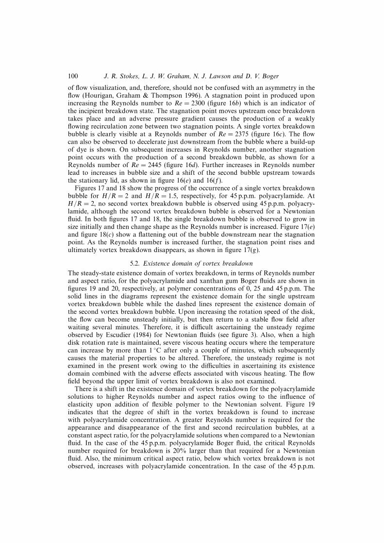
68 J. R. Stokes, L. J. W. Graham, N. J. Lawson and D. V. Boger

Inertia-driven vortex Elasticity-driven vortex

Stationary lid

Secondary flowfield

Rotatinglid/disk

Primary flowfield

Stationarycylinder walls

z

r

h

X

Figure 1. Torsionally driven cavity flow fields.

inertial forces cause the fluid to experience a force directed radially outwards alongthe disk, producing a secondary flow pattern, as shown in the top left-hand cornerof figure 1. This secondary flow vortex is observed for Newtonian fluids and will betermed ‘Newtonian-like’ flow or an ‘inertia driven vortex’. In the case of elastic fluids,normal stresses cause the fluid to experience a force directed radially inwards alongthe disk, opposing centrifugal effects, producing a secondary flow pattern as shownin the top right-hand corner of figure 1. This secondary flow vortex is termed ‘reverseflow’ or an ‘elastic driven vortex’. The competition between inertial and elastic effectscan produce a wide variety of complicated secondary flow fields.

The behaviour of dilute flexible and semi-rigid polymer solutions, with a constantviscosity, in the torsionally driven cavity is investigated. Constant-viscosity elasticliquids, commonly referred to as Boger fluids (Boger 1977/78), are used to ensurethat changes in the flow kinematics are associated purely with fluid elasticity andcannot be confused with effects due to shear-thinning viscosity which are found inall previous experimental work using non-Newtonian fluids in a confined swirlingflow (Hill 1972; Bohme, Rubart & Stenger 1992; Day et al. 1996; Escudier & Cullen1996).

This paper investigates the influence of elasticity in an inertia dominated flow inthe parameter space where vortex breakdown is observed for Newtonian fluids. Part2 (Stokes et al. 2001) investigates the transition from an inertia dominated flow to

Swirling flow of viscoelastic fluids. Part 1 69

an elasticity dominated flow by using several flexible polymer Boger fluids of varyingelasticity levels and a semi-rigid polymer Boger fluid. The aim of the research is toreport on the influence of elasticity in a complex flow field with and without thepresence of inertia. The well-defined boundary conditions of the torsionally drivencavity make it an ideal geometry for the testing of non-Newtonian constitutiveequations for numerical solution as a precursor to solving more difficult and complexswirling flow problems such as those associated with mixing.

2. Previous workThe following section will review previous investigations on the flow behaviour of

both Newtonian and non-Newtonian fluids in the torsionally driven cavity.

2.1. Vortex breakdown and the confined swirling flow of Newtonian fluids

Vortex breakdown refers to the situation where a sudden transition of a vortexflow structure occurs with an abrupt change in character. The breakdown is usuallyassociated with the development of a flow stagnation point and often with regions ofreversed axial flow. Vortex breakdown was reportedly first observed experimentallyas the ‘bursting’ of trailing-edge vortices from aircraft travelling at high angles ofattack by Peckham & Atkinson (1957), Elle (1960), Werle (1960) and Lambourne &Bryer (1961). Detailed investigations of breakdown on delta wings have been limitedby the complicated nature of the leading-edge vortex, its unsteadiness and a lack ofaxial symmetry. Harvey (1962) observed vortex breakdown in a vortex tube whereair travels axially along a circular tube with the degree of swirl imparted on theair controlled by a set of adjustable vanes. The introduction of a diverging tube bySarpakaya (1971) allowed the characterization of several types of breakdown formsand, in particular, he observed the transformation between the two main types ofbreakdown – asymmetric ‘spiral-type’ and axisymmetric ‘bubble-type’ – by increasingthe degree of swirl. The development of more refined experiments allowed the primaryconditions necessary for vortex breakdown to be established as a high degree of swirl,a positive or adverse pressure gradient and a divergence of the stream tubes in thevortex core immediately upstream of the breakdown (Hall 1972). This was investigatedfurther by using an enclosed cylinder with rotating endwall (Escudier 1984). In thiscase, the axisymmetric geometry and well-defined boundary conditions produced awell-posed problem, ideal for the numerical solution of the Navier–Stokes equations(Lopez 1990).

Vortex breakdown has been widely studied over the last 40 years with the firsttheories proposed by Jones (1960), Squire (1960), Ludweig (1961), and Benjamin(1962). Detailed discussion on the mechanisms and theories governing breakdownmay be found in review articles by Hall (1972), Leibovich (1978, 1984), Escudier(1988), and Delerey (1994). More recent discussions on the phenomena have beenmade by Berger & Erlebacher (1995), Keller (1995), Rusak (1996), and Wang & Rusak(1997). However, there is still no general consensus as to the underlying mechanismleading to breakdown.

In the confined cylindrical swirling flow of Newtonian liquids, in which the fluid issituated in an enclosed cylinder with rotating bottom lid (also referred to as a disk orendwall), the rotation of the lid produces a non-uniform centrifugal force along thebase and a secondary flow in the cylinder normal to the primary flow is generated.Here, an Ekman layer is present on the rotating lid with a thickness of the order


X X

X

(c)

(a) (b)

Figure 2. Secondary flow patterns for a Newtonian fluid at conditions showing (a) inertia drivenvortex, (b) pre-incipient breakdown, and (c) vortex breakdown.

(1/Re)0.5 (Lopez 1990) where Re is the Reynolds number defined by:

Re =ρ(2πΩ)R2

η, (1)

where ρ is the density (kg m−3), Ω is the disk rotation rate (s−1), R is the disk radius(m), and η is the viscosity (Pa s). The Ekman layer acts as a centrifugal pump bydriving the fluid outwards along the rotating base, up the sidewalls, inwards alongthe stationary lid and down the central axis in a spiral motion where it is thensucked back into the boundary layer, as depicted in figure 2(a). As the rotation rateof the disk is increased, a widening of the vortex core near the disk is observed witha waviness in the sectional streamline patterns as illustrated in figure 2(b). Furtherincreases in disk speed results in the production of a stagnation point on the centralaxis and a weak recirculation zone which is characteristic of an axisymmetric vortexbreakdown bubble and shown in figure 2(c).

Vortex breakdown in an enclosed cylinder with a rotating lid was first observedexperimentally using flow-visualization techniques by Vogel (1968, 1975), Hill (1972),and Ronnenberg (1977) for a limited range of parameter space and with only onebreakdown bubble observed. Escudier (1984) observed the formation of up to threebreakdown bubbles and produced a detailed diagram, represented in figure 3, showingthe existence domain of vortex breakdown with respect to two governing dimensionlessgroups, the cylinder aspect ratio (H/R) and the Reynolds number defined in (1) whereH is defined as the cylinder height. Escudier (1984) also observed that the breakdown


3 breakdowns

2 breakdowns

Steady

Unsteady

No breakdown

1 breakdown

No breakdown

4000

3500

3000

2500

2000

1500

10001.0 1.5 2.0 2.5 3.0 3.5

H/R

Re

Figure 3. Existence domain of vortex breakdown for Newtonian fluids (Escudier 1984). Circularsymbols represent experimental points produced for a Newtonian fluid in the current paper.

regions were highly axisymmetric, which supported his view that vortex breakdown isinherently axisymmetric and departures from axisymmetry are the result of instabilitiesnot directly associated with the breakdown process. The recirculation zone inside thebreakdown region was observed to contain low interior velocities. An oscillatory flowregime, where the breakdown bubbles move up and down in a periodic manner,was also observed at high Reynolds numbers (above Re ≈ 2600 for H/R > 1.8) withvortex breakdown still highly axisymmetric. The flow was ultimately observed tobecame unsteady and then turbulent with a further increase in the Reynolds number.Fujimura, Koyama & Hyan (1997) examined the location of the stagnation pointsduring spin-up and spin-down of the rotating lid. He found that equilibrium afterspin-up from rest was reached after more than 25 s with conditions 1970 < Re < 2450and H/R = 2.5.

There are only a few reports of measurements of velocity distributions in the diskand cylinder system for Newtonian fluids. In the absence of breakdown, tangentialvelocity measurements have been made by Bien & Penner (1970) and radial andtangential velocity measurements were made by Hill (1972). Prasad & Adrian (1993)have also demonstrated the use of the optical technique stereoscopic particle imagevelocimetry (PIV) to obtain measurements of the tangential, radial and axial velocityprofiles for a Newtonian fluid at low Reynolds number. However, only a limited set ofvelocity measurements have been made in the presence of breakdown by Ronnenberg(1977) and Buchave et al. (1991).

The cylinder with rotating lid provides the simplest geometry in which vortexbreakdown is observed. This flow field is therefore ideal for numerical studies intothe vortex breakdown phenomena using the time-dependent Navier–Stokes equations.Investigation into vortex breakdown at steady-state conditions using the numericalsolution of the axisymmetric Navier–Stokes equations has been primarily performedby Lugt & Abboud (1987), Lopez (1990), Brown & Lopez (1990), Tsitverbilt (1993),and Gelfgat, Bar-Yoseph & Solan (1996). In the work by Lopez (1990), the numericalmodel was validated by comparing the predicted streamlines with the streaklines ob-


Experimentaldye streaklines

Predicted sectionalstreamlines

Figure 4. Comparison between experimetally observed dye-lines (Escudier 1984) and numericallypredicted sectional streamline patterns (Lopez 1990) of vortex breakdown for a Newtonian fluid atRe = 2494 and H/R = 2.5.

served from the flow-visualization images of Escudier (1984) with excellent agreement,as shown in figure 4. Brydon & Thompson (1998) were able to accurately predict theentire existence domain diagram of Escudier (1984).

Lopez (1990) describes the breakdown process as the result of the advection ofangular momentum towards the central axis as the fluid flows radially inwards alongthe stationary lid from the corner of the sidewall at Reynolds numbers a little belowthose required for breakdown (Re ≈ 1600–1800 for H/R = 2.5). Preservation of theangular momentum causes the angular velocity to increase, and consequently anincrease in centrifugal acceleration to a local maxima results as the fluid flows axiallydown in the centre of the cylinder towards the rotating lid. The stream surfacesthen deform and take on a concave shape resulting in a stationary centrifugal (orinertial) wave, as shown in the streamlines of figure 2(b). The amplitude of the inertialwaves increases and their wavelength decreases with further increases towards theReynolds number required for breakdown. The associated axial deceleration is thenlarge enough to cause the flow to stagnate under the crest of the wave and cause anadverse pressure gradient resulting in vortex breakdown (figure 2c).

A ratio of swirl to axial velocity has been well established as a useful criteria forthe breakdown of a vortex (e.g. Hall 1972; Delerey 1994). It indicates that when theswirl (Vφ) is large relative to the axial velocity (Vz), a stagnation point can form, andbreakdown results. The common form of the criteria is as a swirl angle (φν) which isstated by Hall (1972) as:

φν = tan−1

(Vφ

Vz

). (2)

Hall (1972) states that the maximum value of φν upstream of breakdown is invariablygreater than 40 . In the torsionally driven cavity, the numerical analysis of Lugt &Abboud (1987) showed that Hall’s (1972) criteria were met with a value of the swirl


angle just below the stationary lid increasing to 40 once breakdown took place forH/R = 2.

Lopez (1990) and Brown & Lopez (1990) postulated that the recirculation zonesresult from the ‘generation of negative azimuthal vorticity through the stretchingand tilting of vortex lines’ and that this is a necessary condition for the occurrenceof vortex breakdown. They also applied their theory to the swirling pipe flow andestablished an alternative criteria for the occurrence of breakdown based on therelationship between the angle of the velocity vector or swirl angle and the angle ofthe vorticity vector (φω) on stream surfaces upstream of breakdown such that:

φν > φω, (3)

where φω = tan−1(ωφ/ωz) while ωφ and ωz are the azimuthal and radial componentsof vorticity, respectively.

Gelfgat et al. (1996), similarly to Lopez (1990), conclude that a necessary conditionfor vortex breakdown is a concave form of the stream surfaces, which may beconsidered as the cause in the change in sign of the azimuthal component of vorticity.However, Gelfgat et al. (1996) also show that vortex breakdown does not necessarilyoccur when the azimuthal vorticity is negative, or when the stream surfaces areconcave in shape, by observing these conditions at low cylinder aspect ratios wherevortex breakdown does not occur at any Reynolds number.

The oscillatory instability and unsteady flow behaviour which Escudier (1984)observed at high Reynolds number, as shown in figure 3, has been investigated bySørensen & Daube (1989), Lopez (1990), Lopez & Perry (1992), Liao & Young (1995),Sørensen & Christensen (1995), and Gelfgat et al. (1996). The study of time-dependentflows in the torsionally driven cavity flow gives an insight into the changing kinematicsof the various flow structures observed at high Reynolds number.

Related works involving the cylinder geometry include the corotation or counter-rotation of two lids and the use of an open cylinder where a single lid is rotatedwith a free surface. Roesner (1990) investigated experimentally vortex breakdown in acylinder with two rotating lids and found that when at incipient breakdown, corotationof the lids resulted in breakdown while counter-rotation resulted in the disappearanceof the breakdown bubble. Numerical investigations into the two rotating lid systemshave been conducted by Valentine & Jahnke (1994), Lopez (1995), Gelfgat et al.(1996) and Watson & Neitzel (1996). Watson & Neitzel (1996) found that the criteriaof Brown & Lopez (1990) were met at the location of the breakdown bubble in theirflow domain. However, the criteria were not met upstream of breakdown, nor at theincipient state of breakdown, which questions the use of the criteria of Brown &Lopez (1990) as a predictive tool. Spohn, Mory & Hopfinger (1993, 1998) examinedexperimentally the secondary flow in an open cylinder with one rotating lid and foundthat the conditions for vortex breakdown changed noticeably from those observed fora closed cylinder. The differences to the closed cylinder case include: breakdown wasat a lower Reynolds number; a breakdown bubble was present even at the maximumReynolds number tested (Re ≈ 3500); breakdown was observed at aspect ratio aslow as H/R = 0.5; and breakdown bubbles were generally much larger in size. Abreakdown bubble attached to the free surface was also observed which cannot beexplained by classical vortex breakdown theories (e.g. Benjamin 1962; Ludweig 1961)which assumed a cylindrical vortex core upstream of breakdown.

In summary, in the confined swirling flow of Newtonian fluids, inertia causes fluidto be forced outwards along the rotating lid and creates a secondary flow normalto the primary flow. In the subcritical state prior to breakdown, the divergence of


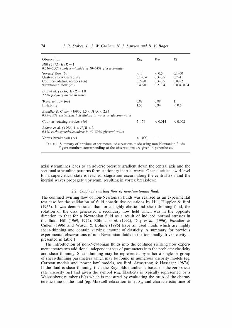
Observation Re0 We El

Hill (1972) H/R = 10.016–0.52% polyacrylamide in 10–54% glycerol–water

‘reverse’ flow (6a) < 1 < 0.5 0.1–60Unsteady flow/instability 0.1–0.4 0.3–0.5 0.7–4Counter-rotating vortices (6b) 0.2–20 0.3–0.5 0.02–2‘Newtonian’ flow (2a) 0.4–90 0.2–0.4 0.004–0.04

Day et al. (1996) H/R = 1.82.5% polyacrylamide in water

‘Reverse’ flow (6a) 0.88 0.88 1Instability 1.57 0.94 < 0.6

Escudier & Cullen (1996) 1.5 < H/R < 2.840.75–1.5% carboxymethylcellulose in water or glucose–water

Counter-rotating vortices (6b) 7–174 < 0.014 < 0.002

Bohme et al. (1992) 1 < H/R < 30.1% carboxymethylcellulose in 60–80% glycerol–water

Vortex breakdown (2c) > 1000 — —

Table 1. Summary of previous experimental observations made using non-Newtonian fluids.Figure numbers corresponding to the observations are given in parentheses.

axial streamlines leads to an adverse pressure gradient down the central axis and thesectional streamline patterns form stationary inertial waves. Once a critical swirl levelfor a supercritical state is reached, stagnation occurs along the central axis and theinertial waves propagate upstream, resulting in vortex breakdown.

2.2. Confined swirling flow of non-Newtonian fluids

The confined swirling flow of non-Newtonian fluids was realized as an experimentaltest case for the validation of fluid constitutive equations by Hill, Huppler & Bird(1966). It was demonstrated that for a highly elastic and shear-thinning fluid, therotation of the disk generated a secondary flow field which was in the oppositedirection to that for a Newtonian fluid as a result of induced normal stresses inthe fluid. Hill (1969, 1972), Bohme et al. (1992), Day et al. (1996), Escudier &Cullen (1996) and Wusch & Bohme (1996) have all used fluids which are highlyshear-thinning and contain varying amount of elasticity. A summary for previousexperimental observations of non-Newtonian fluids in the torsionally driven cavity ispresented in table 1.

The introduction of non-Newtonian fluids into the confined swirling flow experi-ment creates two additional independent sets of parameters into the problem: elasticityand shear-thinning. Shear-thinning may be represented by either a single or groupof shear-thinning parameters which may be found in numerous viscosity models (eg.Carreau models and ‘power law’ models, see Bird, Armstrong & Hassager 1987a).If the fluid is shear-thinning, then the Reynolds number is based on the zero-shearrate viscosity (η0) and given the symbol Re0. Elasticity is typically represented by aWeissenberg number (We) which is measured by evaluating the ratio of the charac-teristic time of the fluid (eg. Maxwell relaxation time: λM and characteristic time of


the process (eg. 1/2πΩ). The Weissenberg number may is evaluated as follows:

We = λM2πΩ. (4)

Another dimensionless number used is the elasticity number (El) which measures theratio of the elastic forces to the inertial forces and may be represented as follows:

El =We

Re=λMη0

ρR2. (5)

A feature of the elasticity number is that it is independent of the rotation rate ofthe lid, provided the relaxation time and viscosity are constant and not shear ratedependent.

Bohme et al. (1992) performed experiments using low concentrations (0.1%) of car-boxymethylcellulose in glycerol–water solvents to produce two highly shear-thinningsolutions in order to investigate the effect of shear-thinning on vortex breakdown. Ashear-thinning parameter (β) which was independent of the rotation rate of the diskwas defined by:

β =ηδ(η0 − ηz)ρτ∗cd2

, (6)

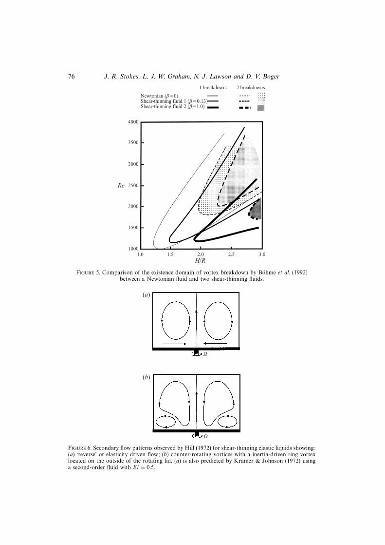
where ηδ is the solvent viscosity, c is the polymer concentration, d is the diameterof the disk, and τ∗ is a constant reference stress which was determined by fitting theviscosity to a master curve. The fluids investigated had shear-thinning parameters ofβ = 0.13 and β = 1.0, with β = 0 indicating a Newtonian fluid. Experiments wereperformed at high Reynolds numbers where inertial dominated and the elasticity wasconsidered negligible, although no measurements of any elastic material propertieswere presented. ‘Newtonian-like’ flow and axisymmetric vortex breakdown were ob-served by Bohme et al. (1992) for the shear-thinning fluids. However, the existencedomain for vortex breakdown decreased in size and was shifted to higher values ofthe cylinder aspect ratio as the degree of shear-thinning was increased. The resultingvortex breakdown domain curves are shown in figure 5 for the two shear-thinningfluids and a Newtonian fluid.

Escudier & Cullen (1996) observed the confined swirling flow of highly shear-thinning carboxymethylcellulose solutions for concentrations of 0.75–1.5% and withReynolds numbers below Re = 174. The primary normal stress difference was mea-sured, but the fluid was considered relatively inelastic because of low values inelasticity number (El < 0.002). At all rotation rates examined, a vortex was observedon the disk which was dominated by inertia such that the secondary flow was inthe ‘Newtonian’ direction and driven outwards along the rotating disk. However, acounter-rotating vortex was observed in the upper portion of the flow cell which wasdriven in the ‘reverse’ direction with a very slow secondary flow velocity and was nearstagnant. An upward flowing jet of fluid containing a wavy structure was also presentin several observations of Escudier & Cullen (1996) along the axis of symmetry.

A range of highly elastic shear-thinning polyacrylamide solutions (0.016–0.52%)were used by Hill (1969, 1972), in solvents of glycerol and water, to examine the effectof elasticity in swirling flow. ‘Reverse’ flow occurred for highly elastic liquids at lowReynolds number where the secondary flow is inwards along the rotating lid againstcentrifugal forces, upwards along the central axis away from the rotating disk andthen along the outside stationary walls, as depicted in figure 6(a). At higher levels ofReynolds number and lower values of elasticity number, complex flow patterns wereobserved where an inertially driven ‘ring’ vortex forms at the edge of the rotating disk,


4000

3500

3000

2000

2500

1500

10001.0 1.5 2.0 2.5 3.0

2 breakdowns:1 breakdown:

Newtonian (b = 0)Shear-thinning fluid 1 (b = 0.13)Shear-thinning fluid 2 (b =1.0)

Re

H/R

Figure 5. Comparison of the existence domain of vortex breakdown by Bohme et al. (1992)between a Newtonian fluid and two shear-thinning fluids.

X

X

(b)

(a)

Figure 6. Secondary flow patterns observed by Hill (1972) for shear-thinning elastic liquids showing:(a) ‘reverse’ or elasticity driven flow; (b) counter-rotating vortices with a inertia-driven ring vortexlocated on the outside of the rotating lid. (a) is also predicted by Kramer & Johnson (1972) usinga second-order fluid with El = 0.5.


counter-rotating with the main ‘reverse’ flow vortex structure, as shown in figure 6(b).Further increases in disk speed caused the growth of the outer edge vortex and thena highly unsteady flow. For low concentrations of polymer (0.03%), Hill (1972) alsoobserved that the secondary flow transformed from ‘reverse’ flow at low Reynoldsnumber to ‘Newtonian-like’ flow at high Reynolds number. Hill (1972) only observed‘Newtonian-like’ flow without any apparent elastic behaviour for concentrations ofpolyacrylamide of 0.015%. The tangential and radial velocities were also measuredfor one highly elastic liquid in the ‘reverse’ flow state.

Day et al. (1996) used a highly elastic shear-thinning polyacrylamide solution(2.5% in water) and observed ‘reverse’ secondary flow at low Reynolds number. Onincreasing the Reynolds number, Day et al. (1996) observed the formation of a ringvortex on the centre of the disk and an instability where the core of the main vortexis observed to spiral with the primary motion of the fluid and is the same as theelastic instability shown in Part 2.

Numerical methods have been used in an attempt to predict the flow patternsobserved for non-Newtonian fluids in confined swirling flow for both elastic andinelastic fluids. The constitutive equations used by Bohme et al. (1992) and Escudier& Cullen (1996) described inelastic fluids while those used by Kramer (1969) andKramer & Johnson (1972), Nirschl & Stewart (1984), and more recently by Chiao &Chang (1990), described elastic fluids.

Bohme et al. (1992) performed a finite-element simulation and used a generalizedNewtonian model in order to model only the shear-thinning viscosity of the fluids heused in his experiments which were mentioned previously for high-Reynolds-numberflow. Vortex breakdown was predicted numerically with reasonable accuracy, but withsome departure from the size and location of the initial breakdown bubble observedexperimentally. Bohme et al. (1992) associated the deviations between the experimentsand numerical prediction as possibly being due to the elasticity of the fluid, whichwas not considered in the constitutive equation used. Escudier & Cullen (1996) usedthe commercial computational fluid dynamics package ‘Polyflow’ with the shear-thinning viscosity described using a generalized Newtonian model which did not takeinto account fluid elasticity. The numerical model predicted only ‘Newtonian-like’flow governing the whole flow cell and did not predict the counter-rotating vorticesobserved in the experiments.

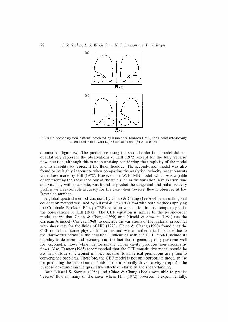
Kramer (1969) and Kramer & Johnson (1972) were the first to try and predict theeffect of elasticity in confined swirling flow and hence reproduce the experimentalobservations made by Hill (1972). Kramer & Johnson (1972) used a perturbationtheory for a weak secondary flow superimposed on an arbitrary primary flow usingboth a second-order fluid model, which assumes a constant viscosity and a constantprimary normal stress coefficient, and the WJFLMB constitutive model of Spriggs,Huppler & Bird (1966), which assumes a power law form of material functionsbut does not account for fluid memory. Figures 6(a) and 7 show the qualitativeobservations made by Kramer & Johnson (1972) when they used the second-orderfluid model for constant Reynolds number and varied the normal stress coefficient,which equated to a variation in the elasticity number of between El = 0 and El = 0.5.As the elasticity number was increased from El = 0 to El = 0.0125, a small elasticallydriven vortex formed on the outer edge of the rotating disk in an otherwise Newtonianflow field (figure 7a). The elastic vortex then governed a majority of the flow fieldwith a further increase in elasticity number to El = 0.025, while only a small inertialvortex remained on the centre of the rotating disk (figure 7b). ‘Reverse’ flow was thenpredicted with an increase in elasticity number to El = 0.5 and elastic effects fully


X

X

(b)

(a)

Figure 7. Secondary flow patterns predicted by Kramer & Johnson (1972) for a constant-viscositysecond-order fluid with (a) El = 0.0125 and (b) El = 0.025.

dominated (figure 6a). The predictions using the second-order fluid model did notqualitatively represent the observations of Hill (1972) except for the fully ‘reverse’flow situation, although this is not surprising considering the simplicity of the modeland its inability to represent the fluid rheology. The second-order model was alsofound to be highly inaccurate when comparing the analytical velocity measurementswith those made by Hill (1972). However, the WJFLMB model, which was capableof representing the shear rheology of the fluid such as the variation in relaxation timeand viscosity with shear rate, was found to predict the tangential and radial velocityprofiles with reasonable accuracy for the case when ‘reverse’ flow is observed at lowReynolds number.

A global spectral method was used by Chiao & Chang (1990) while an orthogonalcollocation method was used by Nirschl & Stewart (1984) with both methods applyingthe Criminale–Ericksen–Filbey (CEF) constitutive equation in an attempt to predictthe observations of Hill (1972). The CEF equation is similar to the second-ordermodel except that Chiao & Chang (1990) and Nirschl & Stewart (1984) use theCarreau A model (Carreau 1968) to describe the variations of the material propertieswith shear rate for the fluids of Hill (1972). Chiao & Chang (1990) found that theCEF model had some physical limitations and was a mathematical obstacle due tothe third-order terms in the equation. Difficulties with the CEF model include itsinability to describe fluid memory, and the fact that it generally only performs wellfor viscometric flows while the torsionally driven cavity produces non-viscometricflows. Also, Tanner (1985) recommended that the CEF constitutive model should beavoided outside of viscometric flows because its numerical predictions are prone toconvergence problems. Therefore, the CEF model is not an appropriate model to usefor predicting the behaviour of fluids in the torsionally driven cavity except for thepurpose of examining the qualitative effects of elasticity and shear-thinning.

Both Nirschl & Stewart (1984) and Chiao & Chang (1990) were able to predict‘reverse’ flow in many of the cases where Hill (1972) observed it experimentally.


Also, the numerical tangential and radial velocity profiles compared very well to themeasurements of Hill (1972) for a ‘reverse’ flow situation. Chiao & Chang (1990)were able to predict a counter-rotating inertially driven vortex on the outer edge ofthe disk (figure 6b) for several of the cases when it was observed experimentally byHill (1972). Contrary to the experiments of Hill (1972), Nirschl & Stewart (1984) didnot predict an inertial vortex on the edge of the disk. Instead, their model predictedthat an inertial vortex would form on the centre of the rotating disk, as did the modelof Kramer & Johnson (1972) at moderate values of elasticity number (figure 7b).In addition, Chiao & Chang (1990) predicted a region of temporal instabilities andchaotic flow which were believed to be consistent with some of the observations madeby Hill (1972) at high Reynolds number.

Wusch & Bohme (1996) used a single-integral constitutive equation (Wagner model)to simulate their own experimental results for a shear-thinning elastic polyacrylamidesolution. Although limited details were presented, the flow patterns were found tobe similar to those observed by Hill (1972). Wusch & Bohme (1996) state that theobserved flow behaviour was qualitatively predicted when the Weissenberg numberwas altered for a set Reynolds number.

The open cylinder with rotating bottom lid was used experimentally for a shear-thinning elastic liquid (25% polyacrylamide (PAA) in water) and a constant-viscosityelastic liquid (silicon oil) by Bohme, Voss & Warnecke (1985). ‘Reverse’ flow wasobserved at low Reynolds number (Re < 0.013 for 2.5% PAA) and a bulge in thefree surface was produced which depended on the primary normal stress difference.The effect was termed the Quelleffekt because the fluid flowed upwards along theaxis of symmetry as a source or Quell. Bohme et al. (1985) developed a second-ordertheory assuming a sufficiently slow flow and solved it using a numerical finite-elementmethod. The results for the surface bulge size agreed well between experiment andthe numerical analysis. It was found that the zero-shear rate normal stress coefficientscould be determined by measuring the displacement of the free surface, and that thesurface tension of the fluid had an insignificant influence on the result. It was alsofound that the axial bulge deformation was quadratic in the angular velocity of therotating disk for low angular velocities. Debbaut & Hocq (1992) used the Oldroyd-Band Johnson–Segalman constitutive models to predict the bulge shape observed byBohme et al. (1985). Both models assume a constant-viscosity for the test fluid anda quadratic dependence of the primary normal stress with shear rate. The secondnormal stress difference is predicted to be zero for the Oldroyd-B model, but it isquantified in the Johnson–Segalman equation such that the relative importance of theprimary and second normal stress differences on the surface bulge could be examined.The surface bulge was found to be larger using the Oldroyd-B model, indicating thatthe primary normal stress difference caused the free surface to rise while the secondnormal stress difference acted against the first normal stress difference as far as thebulge shape was concerned. Good quantitative agreement on surface displacementwas found between the predictions of Debbaut & Hocq (1992) and the experimentsby Bohme et al. (1985). However, Siginer (1991) found that surface tension wasimportant when measuring surface deformation to yield normal stress coefficients. Inaddition, Siginer (1991) predicted sectional streamline patterns with various sets ofcounter-rotating vortices observed which were dependent on the elasticity of the fluidand cylinder aspect ratio.

All previous experimental investigations on the confined swirling flow of non-Newtonian fluids have been performed using shear-thinning elastic liquids, although insome cases the elasticity was considered negligible. When the relaxation time has been


determined for the various fluids, it has also been invariably shear-rate dependent.Both the Reynolds number and the Weissenberg number were consequently evaluatedusing the zero shear-rate value of viscosity and with a shear-rate dependent relaxationtime, respectively. This is despite the fact that the lid may be rotating at substantialrates, and that the magnitudes of the material properties vary throughout the flowcell. Comparison between different experiments and fluids has been difficult owing tothe inability of the Reynolds number, Weissenberg number (or elasticity number) anda shear-thinning parameter to characterize the flow field. If the fluid is shear-thinning,then it is difficult to distinguish between the effects of shear thinning and those ofelasticity, especially when the Reynolds number is high. Consequently, it is difficultto ascertain the role of elasticity in all of the above-mentioned observations. Also,prediction of the flow field for non-Newtonian fluids has not been able to produceall the observations made by Hill (1972) because of the limitations in the constitutiveequations used and/or in the rheological data presented by Hill (1972). However,some good comparisons between experiments and numerical results were found forthe case of ‘reverse’ flow of Hill’s (1972) most elastic fluid. Numerical prediction inconfined swirling flow is possible, but there is a need for experimental results usingwell-characterized fluids which can be described by more sophisticated constitutivemodels than those that have been used previously.

In the present work, the effects of elasticity are isolated by examining the confinedswirling flow of a collection of constant-viscosity elastic liquids (Boger fluids) whichmay be considered as ‘ideal’ fluids. This paper, Part 1, investigates the behaviourof a set of low-viscosity Boger fluids containing up to 75 p.p.m. of either flexiblepolymer (polyacrylamide) or semi-rigid polymer (xanthan gum) when the flow field isdominated by inertia. The effect of the polymer, and hence slight fluid elasticity, onthe existence domain for vortex breakdown will be examined. Part 2 will use mediumto high-viscosity Boger fluids where the inertia is decreased until the flow field is fullydominated by fluid elasticity and viscosity. All the fluids are well characterized suchthat material functions required for various constitutive models may be determined.In particular, the polyacrylamide Boger fluids are ideal for use in the Oldroyd-Bconstitutive model because it requires a constant viscosity and a constant relaxationtime. Radial and axial velocities are measured using particle image velocimetry (PIV)with particular emphasis placed on reporting and comparing the axial velocity profilesalong or near the axis of symmetry. It is envisaged that the results presented will beideal for comparison to numerical predictions in confined swirling flow and will allowtesting of constitutive models and numerical techniques for steady and unsteady flowsof viscoelastic fluids.

3. ExperimentalThe following section describes the confined swirling flow experiment and the

techniques used to measure and visualize the secondary flow field.

3.1. Apparatus

The experimental apparatus, as shown in figure 8 and also described by Day etal. (1996), consisted of an acrylic cylinder with radius 70 ± 0.25 mm, situated in arectangular acrylic water bath, with dimensions 402×402×592 mm3, to reduce imagedistortion effects. The bottom lid of the cylinder was a stainless steel disk which wasrotated using a three-phase a.c. motor via a v-belt and pulley arrangement with aselectable reduction gearbox for the lower disk speed range. The rotation rate of


Central adjustablecylinder (stationary lid)

Perspexouterwalls

Waterbath

Test fluid

Rotating lid shaft

Perspex baseplate

HR

Figure 8. Torsionally driven cavity experimental rig.

the disk was controlled using a variable frequency unit connected to the a.c. motor,and was measured using a frequency counter with a resolution of approximately±0.002 s−1. The stationary top lid was movable and lockable, and positioned accordingto the height to radius ratio required to within ±0.5 mm. Both disk and cylinder weredesigned and built to ensure axial symmetry with the disk rotating with a lateraltolerance of ±50 µm.

Various top lids could be used which depended on the viscosity of the fluid suchthat air bubble entrainment was minimized as the lids were lowered into the fluid andset in place. A lid with one central small capillary hold (0.5 mm diameter), connectedto a needle and a 1 mm diameter tube for dye insertion, was used for fluids witha low viscosity (η < 1.5 Pa s) and it also contained a flush mounted thermocouple.An alternative lid with 5 small holes (1 mm diameter) arranged regularly in a lineacross the lid surface was used for medium-viscosity fluids (1.5 < η < 3 Pa s). A thirdlid with a central small hole (1 mm diameter) and an off-centre large diameter hole(≈ 10 mm diameter), was used for high-viscosity fluids (η > 3 Pa s) such that once thelid was lowered into the fluid, a large flat plug screw could be used to block the hole.Subsequent flow measurements showed that no detectable asymmetries in the flowfield were present for any of the three lids.


During a given experiment, the temperature of the working fluid was found toincrease owing to viscous heating, especially at high rotation rates and for viscousliquids. Therefore, to control the heating effects, the bath water was circulated throughan Haake F3 environmental controller such that most experiments were conductedbetween 20 C and 21 C. For the lids without a flush mounted thermocouple, athermocouple probe could be inserted through the capillary holes in the lids, or alter-natively, for continual measurement it could sit in the capillary holes just outside theflow cell. The temperature of the test fluid was regularly measured to within ±0.05 Csuch that the governing dimensionless numbers could be determined accurately bytaking into consideration temperature variation of the material functions.

3.2. Flow visualization

Illumination of the secondary flow plane was performed using a Coherent Highlightargon-ion laser, operating at 0.5 W, piped through an optical fibre to a cylindricallens. This lens produced a multiline blue–green laser light sheet with a thickness of1–2 mm. Dye flow visualization was conducted in order to observe ‘streaklines’ bydissolving fluorescein powder (≈ 0.2 g l−1) into a small quantity of the test fluid. Thedye was then added via either a syringe–tube–needle arrangement in the centre of thestationary lid for low-viscosity fluids, or by a syringe–tube–capillary arrangement inthe other lids.

Colour photography of the dye streaklines was typically performed at an exposureof 1

4– 1

2s and aperture f2 to f4, using a 35 mm SLR camera with a noct-Nikkor

58 mm lens and 1BUV filter with EPP 100 ISO film. Images were slightly distorted inthe radial direction such that the equivalent radial image distance was 108% of theactual distance at the edge of the field. Video imaging was performed using a SonyHi8 video camera (model DXC537P) with a zoom lens.

3.3. Particle image velocimetry

Velocity data in the secondary flow plane was obtained using the two-dimensionaloptical technique of PIV (Pickering & Halliwell 1985; Adrian 1991). A similar tech-nique, laser speckle velocimetry (LSV), has also been used previously by Binnington,Troup & Boger (1983) to obtain velocity profiles for Boger fluids. PIV was usedin preference to the alternative measurement technique laser-Doppler anemometry(LDA) (Durst, Lehmann & Tropea 1981) owing to the prohibitively long acquisitionperiods that would be required for LDA when measuring the higher viscosity flawswhere in some cases fluid velocities were less than 1 mm s−1.

The following will briefly describe the PIV system which was based on simplemultiple exposure photography for imaging and digital autocorrelation techniquesfor data processing (Adrian 1991; Meinhart, Prasad & Adrian 1993). A detaileddescription of the PIV system can be found in Stokes (1998).

The PIV images were recorded using a pulsed light source from either a 12-sidedrotating mirror system as described by Gray et al. (1991) and shown in figure 9, ora mechanical shutter with light sheet optics. In both cases a 0.5 W argon ion laserlight source was used with a fibre optic delivery and collimation lens. The flow wasseeded using fluorescent rhodamine particles. A Nikon F4 camera with a noct-Nikkor58 mm f1.2 lens was used to record the images onto 35 mm Kodak Tmax400 (TMY)film. The 35 mm transparencies were then digitized into 8 bit greyscale images at aresolution of 2700 d.p.i. by using a Polaroid SprintScan 35 scanner. The processing ofimages was carried out using autocorrelation and post-processing software developedby N.J.L. The software was set up to vary the size of the d.c. peak mask in the


Particles or dyeinjector

Thermocouple

Argon ion laser

Rotatingmirrorcontrolbox

Frequencycounter

Rotatingmirror

Video or35 mm camera

Water bath

Opticalfibre

RH

Figure 9. Torsionally driven cavity experimental set-up showing rotating mirror used for PIVstudies.

correlation plane so that it was proportional to the particle image diameter (Lawson,Coupland & Halliwell 1997).

Figure 10 shows a typical PIV image with corresponding vector map and streamlineplot. The two-dimensional PIV vector maps are measurements of velocity in the axialand radial plane. From this data, a predictor–corrector integration algorithm in thecommercial software package of ‘Tecplot’ was used to obtain streamline traces. Itshould be noted, however, that because of the three-dimensional nature of the flowfield, the streamlines in the following analysis are representative of the ‘instantaneous’flow in the cross-plane and are termed ‘sectional streamline patterns’ (Perry & Steiner1987).

As mentioned previously, the flow field is highly three-dimensional and containsa strong out-of-plane component, termed the azimuthal velocity (Vθ). In the worstcase, this component will displace particles out of the light sheet between exposurescausing data dropout in the vector map. Therefore, areas near the outer surfaces and,in particular, near the rotating disk, were found to have the greatest dropout andonly the central region near the axis of symmetry contained reliable data, where theout-of-plane velocity component was lower. This problem was partly overcome byrecording several PIV images with different pulse separations and then combining thesets of validated data. However, in the case where the secondary flow velocity wasthe same order of magnitude as or greater than the azimuthal velocity component, themajority of PIV vectors were obtained. Other errors were also generated around theaxis of symmetry when particles were displaced across the centre with the primary


(a)

(b)

(c)

140

120

100

80

60

40

20

0–50 0 50

30 mm s–1

z(m

m)

140

120

100

80

60

40

20

0–50 0 50

z(m

m)

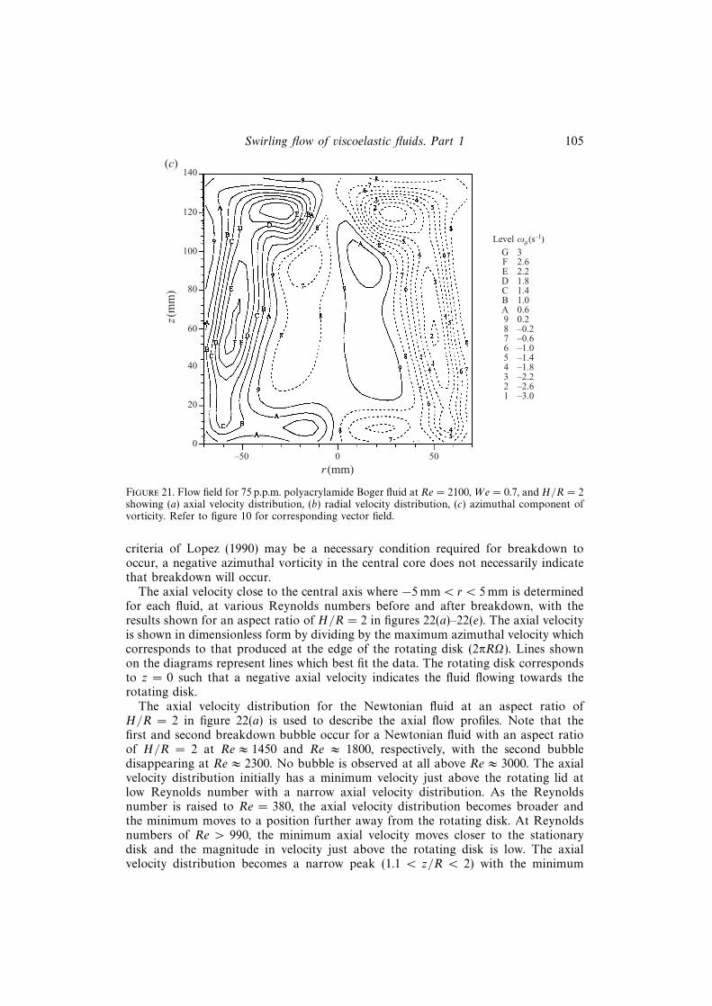
r (mm)

Figure 10. Secondary flow field for 75 p.p.m. polyacrylamide Boger fluid at Re = 2100, We = 0.7,and H/R = 2 showing: (a) PIV image; (b) vector map; (c) sectional streamline patterns.


flow due to either an excessive laser sheet thickness, high velocities in the primaryflow and/or misalignment of the laser sheet position.

The measured radial and axial velocities, given the symbols Vr and Vz , respectively,are made dimensionless for comparative purposes by dividing by a characteristicvelocity. The characteristic velocity is chosen to be the maximum azimuthal velocity(Vθ(max) = 2πΩR) in the system which is located at the edge of the rotating disk. Thecoordinate system is taken as (r, θ, z) with r = 0 and z = 0 corresponding to thecentre of the rotating disk. Therefore, a positive axial velocity corresponds to the fluidflowing upwards, vortically away from the rotating disk. The azimuthal componentof vorticity (ωθ) was determined from the measured velocity data using the followingdefinition:

ωθ =∂νr

∂νz− ∂νz

∂νr. (7)

Components of the rate of strain tensor which could be determined are γrz , γzr, γrr,γθθ, γzz . Only γzz , was used here to give an indication of the strain rate along axialstreamlines about the central axis and was defined by γzz = 2∂νz/∂z.

3.4. Error analysis

For the PIV system, the velocity vector V at any grid point is calculated from acalibrated magnification M, a particle image displacement ∆s and a pulse separation∆t such that:

V =∆s

M∆t. (8)

Therefore, if the uncertainty in measurement of the quantities M, ∆s and ∆t isrepresented by the percentage errors δ(M), δ(∆s) and δ(∆t), respectively, then thetotal percentage error in velocity measurement, δ(V ) can be found from:

δ(V ) =√

[δ(M)]2 + [δ(∆s)]2 + [δ(∆t)]2. (9)

The magnification M (pixels mm−1) was estimated from known image dimensionssuch as the height and diameter of the flow cell, and the error was typically one pixelin 1000 or δ(M) = 0.1%. The maximum deviation in the mirror speed was noted as3 r.p.m. in 167 r.p.m., resulting in a maximum pulse separation error of δ(∆t) = 1.8%.For the error in particle image displacement δ(∆s), previous work by Keane &Adrian (1991) is used to estimate the error from a priori information on the flow. Apriori velocity information is required since the particle displacement error is stronglydependent on spatial velocity gradients (Keane & Adrian 1991) with the worst erroroccurring in the region of highest spatial gradient. From previous work (Lugt &Abboud 1987), the maximum gradient has been predicted at the edge and towardsthe centreline of the flow, and is of the order of 10 mm s−1 across a given interrogationregion of size 1.3 mm. Therefore, with a mean particle image size of 100 µm and amagnification of M = 0.15, the error in particle displacement is estimated to bein the range 2.5% < δ(∆s) < 19.5% for a corresponding range of pulse separations15 ms < ∆t < 143 ms. The total error in measurement from equation (9) will then equal3.1% < δ(V ) < 19.6%. This estimate indicates that it is desirable to keep the laserpulse separation to a minimum owing to the errors generated by velocity gradients.Unfortunately, at lower pulse separations the lower range of secondary flow velocitiescannot be resolved owing to insufficient particle image separations. Hence, a numberof PIV vector maps were taken for a given flow with different pulse separations andthe different sets of validated vectors combined. This technique allows the user to


(a)10

0

–10

–20

–30

–40

–50

–60

–70

–80

0 20 40 60 80 100 120 140

numerical prediction30 ms60 ms100 ms

Pulse time:

Axial distance, z (mm)

Axi

al v

eloc

ity,

Vz(m

m s

–1)

(b)10

0

–10

–20

–30

–40

–50

–60

–70

–80

0 20 40 60 80 100 120 140

numerical result15 ms30 ms60 ms

Pulse time:

Axial distance, z (mm)

Axi

al v

eloc

ity,

Vz(m

m s

–1)

100 ms143 ms

Figure 11. Comparison of the axial velocity along the centreline (r ≈ 0) measured using PIV andthat predicted by Lugt & Abboud (1987) for the Newtonian solvent at (a) Re = 1000, (b) Re = 1500.

restrict the total error in measurement to δ(V ) < 10% and also permits tuning ofthe data to account for the out-of-plane effects mentioned previously. Any remainingnon-valid vectors can then be interpolated and the complete map smoothed to removecorrelation noise.

A comparison is shown in figure 11 between PIV experimental measurements ofthe centreline axial velocity and those predicted using the numerical model of Lugt& Abboud (1987) for a Newtonian fluid at Reynolds numbers of Re ≈ 1000 and


Re ≈ 1500. Each plot shows axial velocities which were determined using a range ofpulse separation times of between 15 ms and 143 ms. The experimental results comparewell to the predicted measurements across the entire length of the cylinder. Deviationsof around 10% between the experimental measurements and those predicted werefound at the minimum peak in axial velocity, about which the velocity gradientswere highest. This deviation matches the level of accuracy predicted in the previouserror analysis and thus gives a sufficient degree of confidence in the technique for thefollowing study of centreline flow fields.

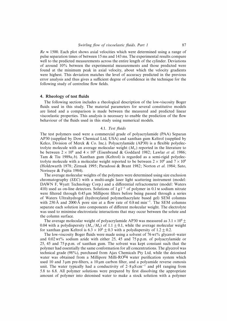
4. Rheology of test fluidsThe following section includes a rheological description of the low-viscosity Boger

fluids used in this study. The material parameters for several constitutive modelsare listed and a comparison is made between the measured and predicted linearviscoelastic properties. This analysis is necessary to enable the prediction of the flowbehaviour of the fluids used in this study using numerical models.

4.1. Test fluids

The test polymers used were a commercial grade of polyacrylamide (PAA) SeparanAP30 (supplied by Dow Chemical Ltd, USA) and xanthan gum Keltrol (supplied byKelco, Division of Merck & Co. Inc.). Polyacrylamide (AP30) is a flexible polyelec-trolyte molecule with an average molecular weight (Mw) reported in the literature tobe between 2× 106 and 4× 106 (Eisenbrand & Goddard 1982; Lawlar et al. 1986;Tam & Tiu 1989a, b). Xanthan gum (Keltrol) is regarded as a semi-rigid polyelec-trolyte molecule with a molecular weight reported to be between 2× 106 and 7× 106

(Holdzwarth 1978; Zirnsak 1995; Paradossi & Brant 1982; Norton et al. 1984; Sato,Norisuye & Fujita 1984).

The average molecular weights of the polymers were determined using size exclusionchromatography (SEC) with a multi-angle laser light scattering instrument (model:DAWN F, Wyatt Technology Corp.) and a differential refractometer (model: Waters410) used as on-line detectors. Solutions of 1 g l−1 of polymer in 0.1m sodium nitratewere filtered through 0.45 µm Millipore filters before being passed through a seriesof Waters Ultrahydrogel (hydroxylated polymethacrylate based gel) SEM columnswith 250 A and 2000 A pore size at a flow rate of 0.8 ml min−1. The SEM columnsseparate each solution into components of different molecular weight. The electrolytewas used to minimise electrostatic interactions that may occur between the solute andthe column surface.

The average molecular weight of polyacrylamide AP30 was measured as 3.1×106±0.04 with a polydispersity (Mw/Mn) of 1.1± 0.1, while the average molecular weightfor xanthan gum Keltrol is 6.3× 106 ± 0.3 with a polydispersity of 1.2± 0.2.

The low-viscosity Boger fluids were made using a solvent of 76 wt% glycerol–waterand 0.02 wt% sodium azide with either 25, 45 and 75 p.p.m. of polyacrylamide or25, 45 and 75 p.p.m. of xanthan gum. The solvent was kept constant such that thepolymer had essentially the same conformation for all concentrations. The glycerol wastechnical grade (98%), purchased from Ajax Chemicals Pty Ltd, while the deionisedwater was obtained from a Millipore Milli-RO

eR4 water purification system whichused 10 and 3 µm pre-filters, a 10 µm carbon filter, and a polyamide reverse osmosisunit. The water typically had a conductivity of 2–8 µS cm−1 and pH ranging from5.8 to 6.8. All polymer solutions were prepared by first dissolving the appropriateamount of polymer into deionised water to make a stock solution with a polymer


Polymer solution Rh(nm) L(nm)

45 p.p.m. PAA 43 —75 p.p.m. PAA 37 —45 p.p.m. XG 85 94475 p.p.m. XG 123 1475

Table 2. PCS measurements of hydrodynamic size of polymers in 76% glycerol.

concentration of 0.1 wt%. The water was warmed to about 30–40 C and the polymerwas added gradually to the water while continually swirling the container in orderto disperse the polymer and avoid agglomeration. Sodium azide was added to thestock solution (< 0.02 wt%) to act as a biocide. The stock solutions were placed ona roller mixer device at very low rotation rates for 12–48 h and, once the polymerwas fully dissolved, the solutions were stored in the refrigerator. The experimentalsolutions were made by adding the appropriate amounts of polymer stock solutionto the required glycerol and sodium azide with the balance made up with deionisedwater. The solutions were then mixed using a four-pronged impeller at low rotationrates for 8–12 h.

4.2. Molecular properties and solution classification

The hydrodynamic size of each polymer in some of the solutions was determinedusing photon correlation spectroscopy (PCS) in a manner similar to that used by Unget al. (1997). Further details of the technique and method used is found in Stokes(1998). The measurements for the hydrodynamic size of polyacrylamide and xanthangum for concentrations of 45 p.p.m. and 75 p.p.m. in 76% glycerol–water are shownin table 2.

The length L of the xanthan gum molecule was determined using relations givenby Broersma (1964) and Young et al. (1978) for rigid rod molecules as follows:

L = Rh

(2σ − 0.19− 8.24

σ+

12

σ2

), (10)

where σ = ln(L/r) is the aspect ratio of a rod and r is the radius of the ‘rigid rod’. Ifr is assumed to be equal to about 2 nm, which is of the same order as that observedin the literature (Zirnsak 1995), then the length of the xanthan gum molecule rangesfrom 944 nm to 1475 nm with an aspect ratio of 472 to 738 for concentrations of45 p.p.m. and 75 p.p.m., respectively.

The intrinsic viscosity was determined for the set of polyacrylamide and xanthangum solutions using viscosity measurements and an automated SCHOTT-GERATEAVS30 intrinsic viscometer using Type 531-10 Ubbelohde viscometer (γw < 40 s−1)and the viscosity measured using rheometry which will be discussed later. The intrinsicviscosity in 76% glycerol was 3.7 l g−1 for the polyacrylamide solutions and 8.2 l g−1

for the xanthan gum solutions (Stokes 1998).The polymer solutions are regarded as dilute when there is no interaction between

molecules. A standard method used to evaluate whether a polymer solution is diluteis to determine a dimensionless concentration of polymer which can be given byeither [η]c (Flory 1960) or cNAV/Mw (Doi & Edwards 1986) where c is the polymerconcentration, NA is Avogadro’s number, and V is the volume occupied by a polymermolecule. Flexible polymers tend to occupy a spherical region in solution such thatV = 4

3πR3

h . In the case of rigid molecules, the spherical region required such that the


large aspect ratio molecule can freely rotate without interaction with its neighboursis calculated from the molecule length such that V = 1

6πL3. The polymer solution is

then regarded as dilute when the dimensionless concentration is less than unity.The dimensionless concentrations for the 75 p.p.m. polyacrylamide solution were

[η]c = 0.28 and cNAV/Mw = 0.005 and, hence, all the polyacrylamide solutions wereconsidered truly dilute using both the criteria of Flory (1960) and Doi & Edwards(1986), respectively. However, for the rigid xanthan gum solution, [η]c = 0.6 whilecNAV/Mw 1, and hence the two criteria are in conflict. Following the criteria ofDoi & Edwards (1986), the xanthan gum solutions are considered semi-dilute.

4.3. Rheology

Steady shear and dynamic property measurements were made using a Carri-MedCSL100 rheometer with a 6 cm diameter plate and 1′ 59′′ cone angle, and a ContravesLow-Shear 40 rheometer equipped with a cup and bob system. The main cup andbob system used with the Contraves was the MS 41S/1S which consisted of a 5.5 mmradius bob with an effective length of 8 mm situated in a 6 mm radius cylinder (cup).The Contraves rheometer, which has a high sensitivity and is designed specifically forlow-viscosity fluids (Tam & Tiu 1989b), was used to measure the properties of thelow-viscosity Boger fluids independently. This was performed by the rheology groupat Nanyang University, Singapore, headed by K. C. Tam. An attempt was made tomeasure the primary normal stress difference using a Weissenberg R19 rheometer butthis was found to be too low to measure. An opposed jet apparatus, the RheometricsRFX, was used to measure an apparent extensional viscosity.

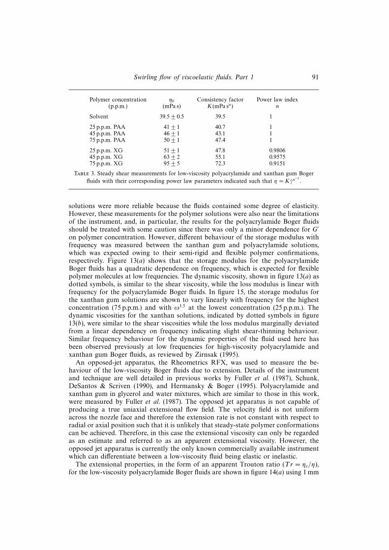
The Carri-Med rheometer was only capable of measuring the viscosity of the low-viscosity Boger fluids for shear rates above about 1–2 s−1, below which the viscositymeasurement was unreliable. The Carri-Med results must be treated with some cautionfor fluids of low viscosity because it measures a higher viscosity than expected atlow shear rates, even for Newtonian fluids, such that an otherwise constant-viscosityfluid appears to be shear-thinning (Lee & Sexton 1994; Stokes 1998). The Contravesrheometer was capable of reliably determining the viscosity of the low-viscosity Bogerfluids for shear rates above 0.1 s−1. The viscosity measured using both rheometers isshown as a function of shear rate in figures 12(a) and 12(b) for the polyacrylamideand xanthan gum low-viscosity Boger fluids, respectively, at 20 C. The Carri-Medresults are distinguished by using dotted symbols, and the Newtonian solvent is shownonly as a straight line for clarity. The measurements from the two rheometers overlapto within a few per cent. Figure 12(a) indicates that each polyacrylamide solutionhas a constant viscosity which is such that there is a linear relationship between theshear stress and shear rate. The behaviour of the xanthan gum solutions, shown infigure 12(b), indicates the presence of slightly shear-thinning viscosity with a deviationfrom a linear shear stress–shear rate relationship. However, for the 75 p.p.m. xanthangum solution which was regarded as the most shear-thinning, the zero shear-rateviscosity was only a factor of two above the infinite shear-rate viscosity and theslope (power-law exponent) of the shear stress–shear rate curve was only 0.92. Theshear thinning parameter was determined using equation (6) to be β = 0.00014 byfitting the viscosity data to the master curve of Bohme et al. (1992). Therefore, incomparison to the fluids used by Bohme et al. (1992), the fluids used in this work canall be considered to have a constant viscosity. The low shear rate value of viscositywas used as the viscosity of all solutions and the results are summarized in table 3.

The dynamic properties of the low-viscosity Boger fluids were too low to be reliablymeasured using the Carri-Med rheometer (Lee & Sexton 1994; Stokes 1998). However,


(a)0.10

0.08

0

0.1 1 10 100 1000

solvent (76% glycerol)

75 p.p.m. PAA

Shear rate (s–1)

0.06

0.04

0.02

45 p.p.m. PAA25 p.p.m. PAA

(b)0.10

0.08

0

0.1 1 10 100 1000

solvent (76% glycerol)

75 p.p.m. XG

Shear rate (s–1)

Vis

cosi

ty, g

(Pa

s)

0.06

0.04

0.02 45 p.p.m. XG25 p.p.m. XG

0.01

Vis

cosi

ty, g

(Pa

s)

Figure 12. Steady shear properties for (a) the low-viscosity polyacrylamide Boger fluids and (b)the low-viscosity xanthan gum Boger fluids, using the Contraves LS40 and Carri-Med CSL100rheometers. Dotted symbols are those measurements obtained from the Carri-Med.

through the use of the Contraves rheometer which has greater sensitivity, the dynamicproperties for the low-viscosity Boger fluids could be measured. The results for thestorage modulus (G′) and dynamic viscosity (η′) as a function of frequency (ω) areshown in figures 13(a) and 13(b) for the polyacrylamide and xanthan gum Bogerfluids, respectively. The storage modulus for the Newtonian solvent was too low toreliably measure (Stokes 1998). The dynamic property measurements for the polymer


Polymer concentration η0 Consistency factor Power law index(p.p.m.) (mPa s) K(mPa sn) n

Solvent 39.5± 0.5 39.5 1

25 p.p.m. PAA 41± 1 40.7 145 p.p.m. PAA 46± 1 43.1 175 p.p.m. PAA 50± 1 47.4 1

25 p.p.m. XG 51± 1 47.8 0.980645 p.p.m. XG 63± 2 55.1 0.957575 p.p.m. XG 95± 5 72.3 0.9151

Table 3. Steady shear measurements for low-viscosity polyacrylamide and xanthan gum Boger

fluids with their corresponding power law parameters indicated such that η = Kγn−1

.

solutions were more reliable because the fluids contained some degree of elasticity.However, these measurements for the polymer solutions were also near the limitationsof the instrument, and, in particular, the results for the polyacrylamide Boger fluidsshould be treated with some caution since there was only a minor dependence for G′on polymer concentration. However, different behaviour of the storage modulus withfrequency was measured between the xanthan gum and polyacrylamide solutions,which was expected owing to their semi-rigid and flexible polymer confirmations,respectively. Figure 13(a) shows that the storage modulus for the polyacrylamideBoger fluids has a quadratic dependence on frequency, which is expected for flexiblepolymer molecules at low frequencies. The dynamic viscosity, shown in figure 13(a) asdotted symbols, is similar to the shear viscosity, while the loss modulus is linear withfrequency for the polyacrylamide Boger fluids. In figure 15, the storage modulus forthe xanthan gum solutions are shown to vary linearly with frequency for the highestconcentration (75 p.p.m.) and with ω1.5 at the lowest concentration (25 p.p.m.). Thedynamic viscosities for the xanthan solutions, indicated by dotted symbols in figure13(b), were similar to the shear viscosities while the loss modulus marginally deviatedfrom a linear dependency on frequency indicating slight shear-thinning behaviour.Similar frequency behaviour for the dynamic properties of the fluid used here hasbeen observed previously at low frequencies for high-viscosity polyacrylamide andxanthan gum Boger fluids, as reviewed by Zirnsak (1995).

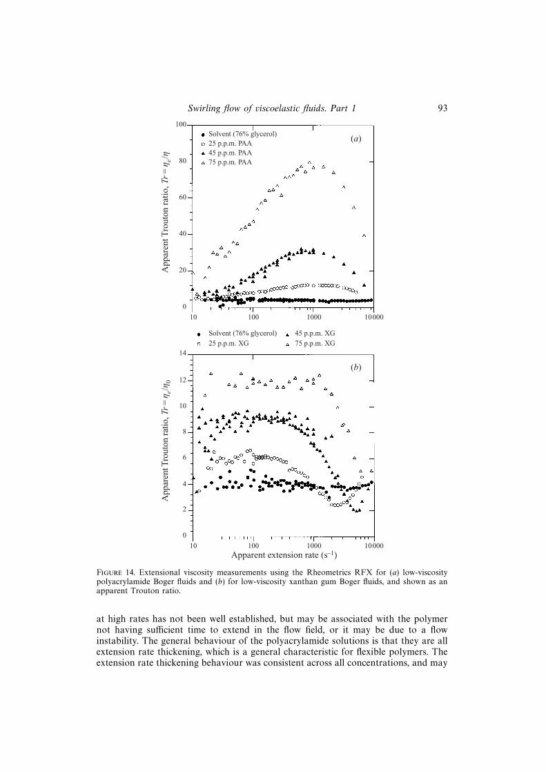
An opposed-jet apparatus, the Rheometrics RFX, was used to measure the be-haviour of the low-viscosity Boger fluids due to extension. Details of the instrumentand technique are well detailed in previous works by Fuller et al. (1987), Schunk,DeSantos & Scriven (1990), and Hermansky & Boger (1995). Polyacrylamide andxanthan gum in glycerol and water mixtures, which are similar to those in this work,were measured by Fuller et al. (1987). The opposed jet apparatus is not capable ofproducing a true uniaxial extensional flow field. The velocity field is not uniformacross the nozzle face and therefore the extension rate is not constant with respect toradial or axial position such that it is unlikely that steady-state polymer conformationscan be achieved. Therefore, in this case the extensional viscosity can only be regardedas an estimate and referred to as an apparent extensional viscosity. However, theopposed jet apparatus is currently the only known commercially available instrumentwhich can differentiate between a low-viscosity fluid being elastic or inelastic.

The extensional properties, in the form of an apparent Trouton ratio (Tr = ηe/η),for the low-viscosity polyacrylamide Boger fluids are shown in figure 14(a) using 1 mm


(a)1

1¬10–1

0.1 1 10 100Frequency, x(rad s–1)

G«(

Pa)

or g

« (Pa

s)

Slope = 2

1¬10–2

1¬10–3

1¬10–4

1¬10–5

(b)1

1¬10–1

0.1 1 10 100Frequency, x(rad s–1)

G«(

Pa)

or g

« (Pa

s)

1¬10–2

1¬10–3

1¬10–4

1¬10–5

Figure 13. Linear viscoelastic properties for (a) the low-viscosity polyacrylamide Boger fluids and(b) the low-viscosity xanthan gum Boger fluids, using the Contraves LS40 rheometer showing thestorage modulus G′ and dynamic viscosity η′ (dotted symbols).

diameter nozzles. The opposed jet apparatus was only capable of measuring a Troutonratio of Tr ≈ 4 for the Newtonian solvent, and not the value of Tr = 3 expectedfor a Newtonian fluid in a true uniaxial extensional flow field. The apparent Troutonratio for the polyacrylamide Boger fluids is initially at a value of Tr ≈ 4 at lowextension rates and then it increases to a maximum at extension rates of ε ≈ 1000 s−1,after which the Trouton ratio decreases. The mechanisms for the apparent decrease


(a)

100

10 100 1000 10000

App

aren

t Tro

uton

rat

io, T

r=

g e/g

Solvent (76% glycerol)

80

60

40

20

0

25 p.p.m. PAA45 p.p.m. PAA75 p.p.m. PAA

(b)

14

10 100 1000 10000Apparent extension rate (s–1)

App

aren

t Tro

uton

rat

io, T

r=

g e/g 0

Solvent (76% glycerol)

12

8

6

4

0

25 p.p.m. XG

45 p.p.m. XG

75 p.p.m. XG

10

2

Figure 14. Extensional viscosity measurements using the Rheometrics RFX for (a) low-viscositypolyacrylamide Boger fluids and (b) for low-viscosity xanthan gum Boger fluids, and shown as anapparent Trouton ratio.

at high rates has not been well established, but may be associated with the polymernot having sufficient time to extend in the flow field, or it may be due to a flowinstability. The general behaviour of the polyacrylamide solutions is that they are allextension rate thickening, which is a general characteristic for flexible polymers. Theextension rate thickening behaviour was consistent across all concentrations, and may


Fluid η0 Ke ne Maximum(Pa s) (Pa s′′) Tr

Solvent 0.0395 0.16 1 4.05

25 p.p.m. PAA 0.041 0.0794 1.32 1245 p.p.m. PAA 0.046 0.162 1.32 3075 p.p.m. PAA 0.050 0.447 1.32 72

25 p.p.m. XG 0.051 0.265 1 6.145 p.p.m. XG 0.063 0.57 1 9.075 p.p.m. XG 0.095 1.11 1 12

Table 4. Extensional viscosity measurements for low-viscosity polyacrylamide and xanthan gum

Boger fluids for 10 < ε < 1000 s−1 with the power law parameters indicated such that: ηe = Keεne−1

.

be expressed using a power law model. A summary of the extensional behaviour ofpolyacrylamide Boger fluids is indicated in table 4.

The apparent Trouton ratio for the xanthan gum Boger fluids is shown in figure14(b) and is relatively constant for extension rates below ε ≈ 1000 s−1, with a summaryof the results indicated in table 4. The area of constant extensional viscosity ischaracteristic of rigid or semi-rigid macromolecules and with perfectly aligned rigidrods. Large-aspect-ratio macromolecules and rigid rods align instantaneously withthe flow field, even at relatively low extension rates, such that the extensional viscosityis relatively independent of extension rate. The xanthan gum solutions, however,show extension rate thinning behaviour at high extension rates (ε > 1000 s−1) whichis similar to that observed for the polyacrylamide solutions. This decrease may meanthat either the macromolecules do not have enough time to align in the flow fieldor there is a flow instability. At extreme extension rates, the apparent Trouton ratiorises again, but this is likely to be due to the anomalies in the instrument discussedpreviously.

The density was measured for the Newtonian solvent and polymer solutions using25 ml calibrated density flasks and was determined to be ρ = 1196± 2 kg m−3 at 20 Cfor all solutions.

4.4. Constitutive model parameters

The polymer relaxation time for several molecular constitutive theories may beestimated using the intrinsic viscosity (see Bird et al. 1987b). For example, the Oldroyd-B constitutive equation, which is suitable to use for the flexible polymers and hencefor the polyacrylamide solutions, may be derived from the elastic dumbbell modelwith the following relation used to determine the longest relaxation time (λ1):

λ1 =[η]ηsMw

RgT(11)

where ηs is the solvent viscosity (Pa s), Rg is the universal gas constant (8.314 J K−1

mol−1), and T is the temperature (K). The retardation time (λ2) in the Oldroyd-Bmodel is given by λ2 = λ1(ηs/η0). The relaxation time in the Maxwell constitutivemodel (λM) is related to the Oldroyd characteristic times by: λM = λ1 − λ2. Thelongest Rouse and Zimm model relaxation times may also be determined, becausethe polymer solutions are dilute, by multiplying the Oldroyd-B relaxation time bythe factors 6π2 and 0.423π2, respectively. Therefore, characteristic relaxation times


Concentration η0 λ1 or λD λ2 λM Elof polymer (mPa s) (s) (s) (s)

Solvent 39.5 — — — —

25 p.p.m. PAA 41 0.186 0.179 0.007 49× 10−6

45 p.p.m. PAA 46 0.186 0.160 0.026 204× 10−6

75 p.p.m. PAA 50 0.186 0.147 0.039 332× 10−6

25 p.p.m. XG 51 0.838 — 0.19 1.65× 10−3

45 p.p.m. XG 63 0.838 — 0.31 3.33× 10−3

75 p.p.m. XG 95 0.838 — 0.58 9.4× 10−3

Table 5. Estimated material properties for the low-viscosity polyacrylamide and xanthan gumBoger fluids.

have been obtained for four constitutive models which are used to describe flexiblemolecules without the need for measurement of the primary normal stress differenceor storage modulus. The viscosity, Oldroyd-B relaxation and retardation times, theMaxwell relaxation time, and the elasticity number are shown for the low-viscositypolyacrylamide Boger fluids in table 5. The Maxwell relaxation time is used asthe characteristic time of the fluid when evaluating the Weissenberg and elasticitynumbers for the fluids used in the torsionally driven cavity.

The validity of using the aforementioned models is demonstrated by predicting thelinear viscoelastic properties using the relaxation times calculated from the intrinsicviscosity. A comparison between the predicted and measured reduced storage modulus(G′R = G′Mw/cRgT ) is shown in figure 15(a) as a function of the reduced frequency(ωR = ωλ1). Only the values predicted for the 75 p.p.m. polyacrylamide solution areshown for clarity with the other concentrations behaving in a very similar manner.A prediction is also shown for the Rouse and Zimm models using data provided byFerry (1980). All of the aforementioned models were able to predict the measured G′Raccurately at medium values of ωR . The measured G′R deviates at low ωR because themeasurements are near the limitations of the rheometer. The Oldroyd-B, Rouse andZimm models fail to predict G′R at high ωR whereas the Maxwell model performedwell across the whole range of ωR . Therefore, the storage modulus for the low-viscositypolyacrylamide Boger fluids has been accurately predicted using the relaxation timecalculated from intrinsic viscosity measurements.

An attempt was made to predict the extensional viscosity measurements usingthe Oldroyd-B and Maxwell models. The models both predict strain rate thickeningbehaviour, which is observed experimentally, but the predicted extensional viscosityasymptotes to infinity when ε = 1/(2λ). The critical extension rate is therefore 2.7 s−1

and 13 s−1 for the Oldroyd-B and Maxwell model, respectively, for the 75 p.p.m.polyacrylamide Boger fluid, and therefore the models are incapable of describing theapparent extensional viscosity measured for the polyacrylamide solutions using theopposed jet apparatus. It also highlights the need to use these models only for flowswhere strain rates are low such that the extensional viscosity is finite.

The rigid-dumbbell constitutive model (see Bird et al. 1987b) may be used to de-scribe rigid or semi-rigid molecules in solution and, hence, was considered appropriateto use for the xanthan gum solutions. The rigid-dumbbell model may use the samerelation for the relaxation time (λD) as that for the elastic dumbbell model, i.e. λD = λ1

where λ1 is given by (12). The rigid dumbbell relaxation time is displayed in table 5


(a)

100

0.001 0.1 10 100

G« R

=G

«M/c

RT

Maxwell model (75 p.p.m.)10

1

0.0001

25 p.p.m. PAA45 p.p.m. PAA75 p.p.m. PAA

0.01 1

0.001

0.01

0.1

Oldroyd-B model (75 p.p.m.)Rouse modelZimm model

xk1

(b)

100

0.1 10 100

G« R

=G

«M/c

RT

rigid dumbbell model10

1

25 p.p.m. XG45 p.p.m. XG75 p.p.m. XG

0.01 1

0.001

0.01

0.1

xkD

Figure 15. Comparison between the measured reduced storage modulus G′R for (a) low-viscositypolyacrylamide Boger fluids and that predicted using selected constitutive models, and (b) thelow-viscosity xanthan gum Boger fluids and that predicted using the rigid-dumbbell constitutivemodel; the relaxation time was calculated from intrinsic viscosity measurement.

for the xanthan gum solutions along with the corresponding Maxwell relaxation time,which was calculated in the same fashion as for the polyacrylamide Boger fluids.

The validity of using a rigid-dumbbell model to describe the low-viscosity xanthangum Boger fluids was tested by comparing the measured values of G′R with thosepredicted in figure 15(b). No concentration dependence for G′R was predicted using


Concentration of xanthan η0 ηe ηe (RD) ηe (RR)gum (p.p.m.) (mPa s) (mPa s) (mPa s) (mPa s)

0 39.5 160 119 11925 51 310 486 13645 63 570 778 15775 95 1110 1221 174

Table 6. Comparison of the apparent extensional viscosity measurements for the xanthan gumBoger fluids and those predicted from the rigid-dumbbell model (RD) of Bird et al. (1987b) andBatchelor’s (1971) theory for semi-dilute perfectly aligned Rigid Rods (RR).

the rigid-dumbbell model. Very good agreement is found between the measured andthe predicted G′R , particularly at low concentrations of xanthan. As the concentrationwas increased, the measured G′R deviates from those predicted as the slope of themeasured G′R-ωR curve decreases. Therefore, deviation of the model from the actualmeasurements may be associated with a departure of the fluids from being a dilutesolution such that as the concentration is raised there is increased interaction betweenmolecules. At high frequency, the rigid-dumbbell model predicts a constant G′R whichis not observed experimentally.

The rigid-dumbbell model of Bird et al. (1987b) and Batchelor’s theory for per-fectly aligned rigid rods (Batchelor 1970, 1971), were used to predict the extensionalbehaviour of xanthan gum. The results (table 6) show that the rigid-dumbbell modelpredictions are in reasonable agreement with the measured extensional viscosity and,hence, the model is suitable for the description of the xanthan gum in extension.

In conclusion, the rheological properties of the low-viscosity Boger fluids used inthis study can be predicted to within an order of magnitude of the experimentalmeasurements using simple constitutive models such as the Oldroyd-B and rigid-dumbbell models. These models were considered reasonably accurate, consideringthat the fluids had a low viscosity and low elasticity. These constitutive models aretherefore recommended for future analytical studies on the torsionally driven cavityflow of the viscoelastic fluids used in this work.

5. ResultsSection 5.1 presents the results obtained using flow visualization and PIV for the

test fluids comprised of 75 p.p.m. or less of polyacrylamide or xanthan gum polymerdissolved in a Newtonian 76% glycerol–water solvent. All fluids have an essentiallyconstant viscosity such that the observed differences in flow behaviour from theNewtonian case are attributed to fluid elasticity associated with the presence ofeither the highly flexible polyacrylamide or the high-aspect-ratio rigid xanthan gummacromolecules. Flow-visualization images using fluorescent dye are initially shownfor the 45 p.p.m. polyacrylamide solution for three sets of cylinder aspect ratios.Section 5.2 examines the effect of polymer, and hence elasticity, on the existencedomain for vortex breakdown. Velocity measurements are shown in § 5.3 to assist inthe establishment of the possible reasons for a change in the flow behaviour whichresults from fluid elasticity and to provide quantitative data suitable for comparisonwith numerical studies.


(a) (b) (c) (d )

(e) ( f )

Figure 16. Flow visualization images for 45 p.p.m. polyacrylamide Boger fluid at H/R = 2.5 for(a) Re = 2015, We = 0.41, (b) Re = 2297, We = 0.47, (c) Re = 2373, We = 0.48, (d) Re = 2443,We = 0.50, (e) Re = 2636, We = 0.54, (f) Re = 2922, We = 0.6.

5.1. Flow visualization

The flow visualization secondary flow patterns for 45 p.p.m. polyacrylamide are illus-trated in figures 16, 17, and 18 for aspect ratios (H/R) of 2.5, 2, and 1.5, respectively.Only the central portion of the secondary flow cell is shown, with correspondingdimensions of 83.9 × 175 mm2, 69.2 × 140 mm2, and 50.6 × 105 mm2 for a H/R of2.5, 2 and 1.5, respectively, to illustrate the changing structure of the vortex core asbreakdown occurs. The flow structures presented are visually similar to those ob-served and described by Escudier (1984) for a Newtonian liquid although the criticalconditions for the occurrence of breakdown are altered owing to the influence of


(a) (b) (c) (d )

(e) ( f ) (g)

Figure 17. Flow visualization images for 45 p.p.m. polyacrylamide Boger fluid at H/R = 2 for(a) Re = 1059, We = 0.22, (b) Re = 1686, We = 0.34, (c) Re = 1760, We = 0.36, (d) Re = 1974,We = 0.40, (e) Re = 3245, We = 0.66, (f) Re = 3442, We = 0.70 (g) Re = 3625, We = 0.74.

elasticity. The secondary flow for the polymer solution is also in the same directionas for a Newtonian fluid.

Figure 16 illustrates the secondary flow patterns for 45 p.p.m. polyacrylamide at anaspect ratio of H/R = 2.5. At low Reynolds numbers, a straight line of dye flowsdown the centreline into the Ekman boundary layer and is recirculated outwardsalong the rotating disk, up the sidewalls, along the stationary lid and down thecentral vortex core once again. However, as the Reynolds number is increased toRe = 2015 (figure 16a), wavy dye streak lines are observed around the centreline, andwhat appears like a spiral on the centreline. A spiral of dye is usually observed atReynolds numbers just below those required to cause breakdown and is an artefact


of flow visualization, and, therefore, should not be confused with an asymmetry in theflow (Hourigan, Graham & Thompson 1996). A stagnation point in produced uponincreasing the Reynolds number to Re = 2300 (figure 16b) which is an indicator ofthe incipient breakdown state. The stagnation point moves upstream once breakdowntakes place and an adverse pressure gradient causes the production of a weaklyflowing recirculation zone between two stagnation points. A single vortex breakdownbubble is clearly visible at a Reynolds number of Re = 2375 (figure 16c). The flowcan also be observed to decelerate just downstream from the bubble where a build-upof dye is shown. On subsequent increases in Reynolds number, another stagnationpoint occurs with the production of a second breakdown bubble, as shown for aReynolds number of Re = 2445 (figure 16d). Further increases in Reynolds numberlead to increases in bubble size and a shift of the second bubble upstream towardsthe stationary lid, as shown in figure 16(e) and 16(f).

Figures 17 and 18 show the progress of the occurrence of a single vortex breakdownbubble for H/R = 2 and H/R = 1.5, respectively, for 45 p.p.m. polyacrylamide. AtH/R = 2, no second vortex breakdown bubble is observed using 45 p.p.m. polyacry-lamide, although the second vortex breakdown bubble is observed for a Newtonianfluid. In both figures 17 and 18, the single breakdown bubble is observed to grow insize initially and then change shape as the Reynolds number is increased. Figure 17(e)and figure 18(c) show a flattening out of the bubble downstream near the stagnationpoint. As the Reynolds number is increased further, the stagnation point rises andultimately vortex breakdown disappears, as shown in figure 17(g).

5.2. Existence domain of vortex breakdown

The steady-state existence domain of vortex breakdown, in terms of Reynolds numberand aspect ratio, for the polyacrylamide and xanthan gum Boger fluids are shown infigures 19 and 20, respectively, at polymer concentrations of 0, 25 and 45 p.p.m. Thesolid lines in the diagrams represent the existence domain for the single upstreamvortex breakdown bubble while the dashed lines represent the existence domain ofthe second vortex breakdown bubble. Upon increasing the rotation speed of the disk,the flow can become unsteady initially, but then return to a stable flow field afterwaiting several minutes. Therefore, it is difficult ascertaining the unsteady regimeobserved by Escudier (1984) for Newtonian fluids (see figure 3). Also, when a highdisk rotation rate is maintained, severe viscous heating occurs where the temperaturecan increase by more than 1 C after only a couple of minutes, which subsequentlycauses the material properties to be altered. Therefore, the unsteady regime is notexamined in the present work owing to the difficulties in ascertaining its existencedomain combined with the adverse effects associated with viscous heating. The flowfield beyond the upper limit of vortex breakdown is also not examined.

There is a shift in the existence domain of vortex breakdown for the polyacrylamidesolutions to higher Reynolds number and aspect ratios owing to the influence ofelasticity upon addition of flexible polymer to the Newtonian solvent. Figure 19indicates that the degree of shift in the vortex breakdown is found to increasewith polyacrylamide concentration. A greater Reynolds number is required for theappearance and disappearance of the first and second recirculation bubbles, at aconstant aspect ratio, for the polyacrylamide solutions when compared to a Newtonianfluid. In the case of the 45 p.p.m. polyacrylamide Boger fluid, the critical Reynoldsnumber required for breakdown is 20% larger than that required for a Newtonianfluid. Also, the minimum critical aspect ratio, below which vortex breakdown is notobserved, increases with polyacrylamide concentration. In the case of the 45 p.p.m.


polyacrylamide Boger fluid when compared to the Newtonian solvent, the minimumcritical aspect ratio for the first breakdown bubble increases by approximately 20%.However, the minimum critical aspect ratio for the second breakdown bubble increasesby about the same absolute magnitude as that for the first breakdown bubble. Theupper domain curves, where the single vortex breakdown bubble disappears, for eachpolyacrylamide concentration merge to a common curve and are offset at greaterReynolds numbers than for the Newtonian fluid. Vortex breakdown is not observedat all for 75 p.p.m. polyacrylamide for aspect ratios below H/R = 2.8.

The vortex breakdown existence domain is also altered by semi-rigid xanthangum as shown for polymer concentrations of 25 and 45 p.p.m. in figure 20. Thearea bounded by the vortex breakdown domain curves decreases with increasingxanthan concentration and no second breakdown bubble is observed at aspect ratiosbelow H/R = 2.5 for the 45 p.p.m. xanthan gum. There is only a slight increasein the Reynolds numbers corresponding to the formation of the first breakdownbubble and a decrease in the Reynolds numbers corresponding to the disappearanceof the first and second breakdown bubble with increasing xanthan concentration.This corresponds to about a 25% decrease in Reynolds numbers required for thedisappearance of the first breakdown bubble for the 45 p.p.m. xanthan gum Bogerfluid. There is also a small shift (≈ 5%) to higher Reynolds numbers for the occurrenceof the second breakdown bubble for the 25 p.p.m. xanthan gum Boger fluid. Thexanthan gum also causes the minimum critical aspect ratio required for breakdownto increase with polymer concentration to a high as about 40% for the 45 p.p.m.xanthan gum solution. Vortex breakdown is not observed for aspect ratios of lessthan H/R = 2.8 for 75 p.p.m. xathan gum.

It should be noted that the xanthan gum solutions are slightly shear-thinning aboveshear rates of γ ≈ 1–10 s−1, while the Reynolds number is based on the zero shear-rate viscosity. For the overall flow kinematics, the degree of shear-thinning for thexanthan solutions is considered negligible when it is compared to the highly shear-thinning fluids of Bohme et al. (1992). The shear-thinning parameter for the 75 p.p.m.xanthan gum Boger fluid is β = 0.00014, whereas for the fluids of Bohme et al. (1992),β > 0.13. The major effect of shear-thinning in the experiments of Bohme et al. (1992)was to increase the minimum critical aspect ratio required for breakdown. Therefore,with values of the shear-thinning parameters close to zero, the slight shear-thinningbehaviour of the xanthan gum Boger fluids will have no effect on the minimumcritical aspect ratio required for breakdown. Hence, the only effect of the slight shear-thinning behaviour of the xanthan gum solutions is the difficulty associated withdefining a viscosity to use in the Reynolds number. By defining the viscosity as thezero shear-rate value, the Reynolds number will be underestimated, considering thatthe flow kinematics are governed by shear rates above γ ≈ 1 s−1 since the rotationrate of the disk is generally greater than Ω ≈ 1 s−1. If a lower viscosity is used todefine the Reynolds number for the xanthan solutions, then the Reynolds numberwill be larger than those reported here. This causes the vortex breakdown domaincurves for the xanthan gum solutions to be shifted to higher Reynolds numbers andtherefore be similar to the domain curves for the polyacrylamide Boger fluids.

5.3. Velocity measurements

Particle image velocimetry has been used to determine the axial and radial velocityfield in the secondary flow plane for the Newtonian solvent and the 45 and 75 p.p.m.polyacrylamide and xanthan gum Boger fluids. A typical vector field and sectionalstreamline plot for the 75 p.p.m. polyacrylamide Boger fluid is shown in figure 10


(a) (b) (c) (d )

Figure 18. Flow visualization images for 45 p.p.m. polyacrylamide Boger fluid at H/R = 1.5 for(a) Re = 1403, We = 0.29, (b) Re = 1574, We = 0.32, (c) Re = 1808, We = 0.37, (d) Re = 1959,We = 0.40.

for the case of a Reynolds number of Re = 2100 and an aspect ratio of H/R = 2.At these conditions, vortex breakdown is observed for a Newtonian fluid but it issuppressed for the 75 p.p.m. polyacrylamide Boger fluid. The axial and radial velocityprofiles are shown in figure 21 as contour plots where solid lines indicate a positivevelocity while dashed lines indicate a negative velocity noting that the origin is locatedat the centre of the rotating disk. The velocity is constant along a contour line withthe absolute velocity given alongside the diagrams.

The secondary flow for the 75 p.p.m. polyacrylamide Boger fluid is examined usingthe vector plot and velocity contour diagrams in figures 10 and 21, respectively.Starting from the origin in the middle of the rotating disk, fluid is quickly pumpedoutwards along the disk to the stationary sidewalls. The radial velocity (figure 21b)shown in the region closest to the disk is difficult to visualize, and, therefore, thevelocity in this region is high in error, as discussed in § 3.4. Fluid then flows upwardalong the stationary sidewall, with a peak in velocity of around −32 mm s−1 (figure21a), before turning inwards as it encounters the top stationary lid. The fluid thenflows inwards along the stationary lid with a similar radial velocity to that presentalong the rotating disk (figure 21b). The fluid then flows down the central regionwhere it passes through a peak in the axial velocity of more than 32 mm s−1 at aheight of z = 120 mm for a radius of r = ±15 mm s−1 (figure 21a). The fluid then slowsdown as it moves down the central axis to a region of almost constant axial velocityfor z < 100 mm with −12 < Vz < −16 mm s−1 before passing through another smallpeak at z ≈ 15 mm. The flow along the central core region is dominated by the axialvelocity with only small radial fluctuations indicated at z ≈ 100 mm, which resultsfrom the divergence of the streamlines (figures 10 and 21b).

A contour diagram of the azimuthal component of vorticity is shown in figure 21(c)with a positive vorticity indicated as that directed into the page. In the left-hand halfof figure 21(c), there is an area of negative azimuthal vorticity near the central axiswhich, according to Lopez (1990), is a necessary condition for vortex breakdown to


4000

3500

3000

2500

2000

1500

10001.0 1.5 2.0 2.5

Newtonian25 p.p.m. PAA45 p.p.m. PAA

Re

H/R

Figure 19. Existence domain for vortex breakdown of low-viscosity polyacrylamide Boger fluidsand the Newtonian solvent (76% glycerol). Solid line and filled symbols: 1 breakdown. Dashed line,open symbols and shaded area: 2 breakdowns.

3500

3000

2500

2000

1500

10001.0 1.5 2.0 2.5

Newtonian25 p.p.m. XG45 p.p.m. XG

Re

H/R

Figure 20. Existence domain for vortex breakdown of low-viscosity xanthan gum Boger fluids andthe Newtonian solvent (76% glycerol). Solid line and filled symbols: 1 breakdown. Dashed line,open symbols and shaded area: 2 breakdowns.


140

120

100

80

60

40

20

0

–50 0 50

HGFEDCBA987654321

322824201612

840

–4–8

–12–16–20–24–28–32

Level Vz (mm s–1)

z(m

m)

(a)

140

120

100

80

60

40

20

0–50 0 50

CBA987654321

22181410

62

–2–6

–10–14–18–22

Level Vr (mm s–1)

z(m

m)

(b)

r (mm)

Figure 21 (a, b). For caption see facing page.

occur. The streamlines and vector plot in figure 10 indicate that the streamlines havea concave form, which is also considered a necessary condition before breakdownoccurs. Yet, vortex breakdown is not observed at any Reynolds number at this aspectratio for the 75 p.p.m. polyacrylamide Boger fluid which suggests that although the


140

120

100

80

60

40

20

0–50 0 50

GFEDCBA987654321

32.62.21.81.41.00.60.2–0.2–0.6–1.0–1.4–1.8–2.2–2.6–3.0

Level xh (s–1)

z(m

m)

(c)

r (mm)

Figure 21. Flow field for 75 p.p.m. polyacrylamide Boger fluid at Re = 2100, We = 0.7, and H/R = 2showing (a) axial velocity distribution, (b) radial velocity distribution, (c) azimuthal component ofvorticity. Refer to figure 10 for corresponding vector field.

criteria of Lopez (1990) may be a necessary condition required for breakdown tooccur, a negative azimuthal vorticity in the central core does not necessarily indicatethat breakdown will occur.

The axial velocity close to the central axis where −5 mm < r < 5 mm is determinedfor each fluid, at various Reynolds numbers before and after breakdown, with theresults shown for an aspect ratio of H/R = 2 in figures 22(a)–22(e). The axial velocityis shown in dimensionless form by dividing by the maximum azimuthal velocity whichcorresponds to that produced at the edge of the rotating disk (2πRΩ). Lines shownon the diagrams represent lines which best fit the data. The rotating disk correspondsto z = 0 such that a negative axial velocity indicates the fluid flowing towards therotating disk.

The axial velocity distribution for the Newtonian fluid at an aspect ratio ofH/R = 2 in figure 22(a) is used to describe the axial flow profiles. Note that thefirst and second breakdown bubble occur for a Newtonian fluid with an aspect ratioof H/R = 2 at Re ≈ 1450 and Re ≈ 1800, respectively, with the second bubbledisappearing at Re ≈ 2300. No bubble is observed at all above Re ≈ 3000. The axialvelocity distribution initially has a minimum velocity just above the rotating lid atlow Reynolds number with a narrow axial velocity distribution. As the Reynoldsnumber is raised to Re = 380, the axial velocity distribution becomes broader andthe minimum moves to a position further away from the rotating disk. At Reynoldsnumbers of Re > 990, the minimum axial velocity moves closer to the stationarydisk and the magnitude in velocity just above the rotating disk is low. The axialvelocity distribution becomes a narrow peak (1.1 < z/R < 2) with the minimum


0

0.02

–0.02

0 0.5

Axi

al v

eloc

ity,

Vz/

2pX

R

–0.04

–0.06

–0.08

–0.10

–0.121.0 1.5 2.0

380990129015102144

Re

0

0.02

–0.02

0 0.5

Axi

al v

eloc

ity,

Vz/

2pX

R

–0.04

–0.06

–0.08

–0.10

–0.121.0 1.5 2.0

36592013001890

Re

0

0.02

–0.02

0 0.5

Axi

al v

eloc

ity,

Vz/

2pX

R

–0.04

–0.06

–0.08

–0.10

–0.121.0 1.5 2.0

390712106713221780

Re

(a)

(b)

(c)

Axial distance, z/R

Figure 22 (a–c). For caption see facing page.


0

0.02

–0.02

0 0.5

Axi

al v

eloc

ity,

Vz/

2pX

R

–0.04

–0.06

–0.08

–0.10

–0.121.0 1.5 2.0

380105015702100

Re

0

0.02

–0.02

0 0.5

Axi

al v

eloc

ity,

Vz/

2pX

R

–0.04

–0.06

–0.08

–0.10

–0.121.0 1.5 2.0

240520

10501580

Re

(d )

(e)

Axial distance, z/R

830

Figure 22. Dimensionless axial velocity measurements along centreline (r ≈ 0) for (a) Newtoniansolvent (76% glycerol), (b) 45 p.p.m. polyacrylamide Boger fluid where El = 49× 10−6, (c) 45 p.p.m.xanthan gum Boger fluid where El = 3.33 × 10−3, (d) 75 p.p.m. polyacrylamide Boger fluid whereEl = 332× 10−6, (e) 75 p.p.m. xanthan gum Boger fluid where El = 9.4× 10−3. H/R = 2.0.

close to the stationary lid as the Reynolds number is raised to Re = 1290. This peakcorresponds to the stage just prior to breakdown. The velocity near the rotating lidis small in magnitude with a flat distribution governing a majority of the axial length(z/R < 1.1). This low velocity or almost stagnant region continues to migrate to ahigher axial length until a stagnation point arises and a small region of flow reversaloccurs which indicates the occurrence of vortex breakdown. This vortex breakdownis shown for Re = 1510 where a positive velocity is indicated at z/R = 1.3. Abovez/R = 1.3, the axial velocity peak has become narrower and the magnitude of theminimum axial velocity has decreased slightly from its value prior to breakdown. Twobreakdown bubbles are observed at higher Reynolds numbers such as in the case of


Re = 2144 and the magnitude of the minimum axial velocity is less than about halfof that prior to breakdown.

The progression of the axial velocity distribution for 45 p.p.m. polyacrylamide and45 p.p.m. xanthan gum Boger fluids are very similar to those of the Newtonian solventwith the measurements shown in figures 22(b) and 22(c), respectively. As previouslymentioned, vortex breakdown occurs at larger Reynolds numbers for the 45 p.p.m.polyacrylamide Boger fluids than for the Newtonian solvent and this is reflectedin the velocity profiles. At the same Reynolds number, the velocity profile for thepolyacrylamide solution is less developed than that for the Newtonian fluid such thatto obtain a similar velocity distribution, a higher Reynolds number is required forthe polyacrylamide Boger fluid. A similar Reynolds number is required for vortexbreakdown of the xanthan gum solution compared with the Newtonian solvent whichis also reflected by similar velocity profiles at similar Reynolds numbers in the twocases. However, the most significant difference in the axial velocity profiles is that theminimum velocity for both the 45 p.p.m. polymer Boger fluids is lower in magnitudethan for the Newtonian solvent. Prior to breakdown, the minimum velocity for theNewtonian fluids is approximately a constant of value of Vz/(2πRΩ) ≈ −0.11 for380 < Re < 1290 and seemingly independent of aspect ratio for 1.5 < H/R < 2.5.However, in comparison to the Newtonian fluid, the minimum velocities were 13%and 27% lower with values of Vz/(2πRΩ) ≈ −0.096 and Vz/(2πRΩ) ≈ −0.08 forthe 45 p.p.m. polyacrylamide and 45 p.p.m. xanthan gum Boger fluids, respectively,prior to breakdown. This decrease in magnitude of the minimum velocity correlateswith the 20% and 40% increase in the minimum aspect ratio required for vortexbreakdown to occur for the 45 p.p.m. polyacrylamide and 75 p.p.m. xanthan gumBoger fluids, respectively. As displayed in the existence domain plots in figures 19and 20, the minimum aspect ratios for the Newtonian, 45 p.p.m. polyacrylamideand 45 p.p.m. xanthan gum Boger fluids was about 1.25, 1.5 and 1.75, respectively.Therefore, the results indicate that there is a strong connection between the magnitudeof the minimum velocity and the minimum aspect ratio required for breakdown tooccur.

Vortex breakdown does not occur for the 75 p.p.m. polyacrylamide or 75 p.p.m.xanthan gum Boger fluids for aspect ratios equal to or less than H/R = 2.8. Thevelocity distributions for these two Boger fluids are shown in figures 22(d) and 22(e),respectively. While showing a similar progression to the velocity profiles for theNewtonian solvent, the Boger fluids in this case do not reach very low minimum axialvelocities and the velocity distributions are flatter when compared to the previouscases. There is no longer a sharp peak in the axial velocity at Reynolds numbers wherevortex breakdown would occur for the Newtonian fluid. At Reynolds numbers ofRe ≈ 1500–1600, the velocity distribution for the Newtonian fluid (figure 22a) passesthrough a sharp minimum at z/R ≈ 1.7 to Vz/(2πRΩ) ≈ −0.084 before increasingto a positive value in the location of the breakdown bubble at z/R ≈ 1.3. However,the velocity distributions for the polyacrylamide (figure 22d) and xanthan (figure22e) Boger fluids do not have a sharp minimum peak and the minimum velocitiesare 67% and 86% lower in magnitude than for the Newtonian case. For Re ≈1500–1600, the minimum axial velocity for the polyacrylamide Boger fluid was onlyVz/(2πRΩ) ≈ −0.028 at an aspect ratio of z/R ≈ 1.3, while the minimum velocityfor the xanthan gum Boger fluid is only Vz/(2πRΩ) ≈ −0.012 at an aspect ratio ofz/R ≈ 1.975. Therefore, the results suggest that the total suppression of breakdownfor these two Boger fluids is due to the reduced magnitude of the peak axial velocitywhich has been caused by the action of elasticity.


140

120

100

80

60

40

20

0

–50 0 50

r (mm)

z(m

m)

(a)

GFEDCBA987654321

2.42.081.761.441.120.80.480.16–0.16–0.48–0.8–1.12–1.44–1.76–2.08–2.4

Level crr(s–1)

.

140

120

100

80

60

40

20

0–50 0 50

r (mm)

z(m

m)

(b)

IHGFEDCBA987654321

3.432.62.21.81.41.00.60.2–0.2–0.6–1.0–1.4–1.8–2.2–2.6–3.0–3.4

Level czz(s–1)

.

Figure 23. Flow field for 75 p.p.m. polyacrylamide Boger fluid at Re = 2100, We = 0.7, and H/R = 2showing the following components of the rate-of-strain tensor (a) γrr and (b) γzz . Refer to figures10 and 26 for corresponding vector field and velocity distributions, respectively.


6. Discussion

The confined swirling flow has been dramatically affected owing to the additionof dilute and semi-dilute concentrations of high molecular weight polymers of bothflexible and semi-rigid conformation, respectively, to a Newtonian solvent. The criticalaspect ratio for the occurrence of vortex breakdown is shifted to greater values asthe concentration of the polymer was increased. Vortex breakdown is not observedusing 75 p.p.m. of polyacrylamide or 75 p.p.m. xanthan gum for the aspect ratiosexamined (H/R < 2.8). Velocity measurements have indicated that the shift in thecritical aspect ratio and ultimate suppression of breakdown has arisen because of thelowering of the maximum magnitude of the dimensionless axial velocity along thecentreline (r ≈ 0). The mechanisms by which elasticity has affected the axial velocityand the suppression of vortex breakdown is now discussed in more detail.

Normal stresses induced in flow arise as a result of fluid elasticity. In swirling flow,normal stresses cause a tension along curvilinear streamlines with a resultant forceacting inwards, against the outward normal of these curved streamlines and in theopposite direction to inertial forces. Although the primary normal stress differenceis not measurable for the low-viscosity Boger fluids, it may be estimated from thestorage modulus using the relation:

Limγ→0NI/2γ2 ≡ Limω→0G

′/ω2

(see Bird et al. 1987a). Therefore, the radial velocity in the governing boundary layerpositioned on the rotating disk, which drives the whole secondary flow, is reducedby the action of normal stresses. A slight reduction in the radial velocity out ofthe governing boundary layer will result in a lower axial velocity down the cen-treline out of the boundary layer located on the stationary top lid. The wavinessobserved in the sectional streamlines prior to breakdown (figure 2b) results frominertial fluctuations referred to as inertial waves. These inertial waves are consideredcritical for the occurrence of breakdown, and their degree of waviness is controlledby the upstream axial velocity. A decrease in the axial velocity magnitude from thestationary lid therefore leads to a reduction and suppression of the degree of the wavi-ness in the sectional streamlines and subsequently hinders the occurrence of vortexbreakdown.

Extensional effects often play a role in phenomena associated with viscoelastic flu-ids, such as in drag reduction where extensional viscosity is associated as the cause inthe reduction of turbulence through the suppression of eddy formation. It is, therefore,expected that extensional viscosity will play a role in the suppression of vortex break-down. The apparent Trouton ratio for the Boger fluids was significantly greater thanthe Newtonian Trouton ratio of Tr = 3, as shown in § 4.3. The polyacrylamide Bogerfluids are strain rate thickening while the extensional viscosity of the xanthan gumBoger fluids is constant with strain rate. Therefore, at even small extension rates, theresistance to extension from the xanthan gum Boger fluids is higher than for Newton-ian fluids and this will have an effect on the flow kinematics. For the polyacrylamideBoger fluid, reasonable extension rates are required for the extensional viscosity tobe above the Newtonian value owing to its strain rate thickening behaviour. Figure23 shows two components of the rate-of-strain tensor in the secondary flow plane,namely γrr and γzz , for the 75 p.p.m. polyacrylamide Boger fluid at Re = 2100. Dashedlines represent areas of negative strain rate (compressive) and solid lines representareas of positive strain rate (extension). The areas of highest extension are situatedjust below the stationary lid with γzz ≈ 3.4 s−1 and along the stationary walls from the


corner of the rotating disk where z < 50 mm with γzz ≈ 2.2 s−1. These areas will showthe highest resistance to extension in the secondary flow field for the polyacrylamideBoger fluids. The greater resistance to extension for the Boger fluids when comparedto Newtonian fluids will result in a lowering of the velocity in areas of high extensionrate. In particular, the minimum velocity along the centreline would be suppressed, asobserved in the velocity profiles for 75 p.p.m. polyacrylamide and 75 p.p.m. xanthangum Boger fluids in figures 22(d) and 22(e).

It is clear that even a small degree of elasticity can change the character of a swirlingflow field dramatically, even when it is dominated by inertial forces. Predictions of theflow of non-Newtonian fluids are limited, including when inertia is negligible or wheninertial effects are high, such as in turbulent or swirling flows. The experiments in thispaper were carried out to provide experimental observations and quantitative datain a well-defined flow field, using well-characterized fluids, in order to examine theeffect of elasticity on an established steady flow phenomenon observed for Newtonianfluids. As reviewed previously, inertia is the dominant force governing the flow, and,hence, the confined swirling flow experiment has demonstrated a suitable test case forvalidation of non-Newtonian constitutive models. This validation process is a preludeto predicting other inertia-dominated flows such as those encountered in mixingprocesses and drag reduction. Part 2 will examine the secondary flow field, as inertiais gradually removed from the problem and the flow becomes heavily dominated byelastic forces.

7. ConclusionThe secondary flow of low-viscosity dilute polyacrylamide and xanthan gum solu-

tions has been significantly altered when compared to a Newtonian solution of similarconstant viscosity. When compared to observations in the confined swirling flow ofNewtonian fluids, the critical aspect ratio for the occurrence of vortex breakdownhas been shifted to greater values with increasing polymer concentration such thatbreakdown was not observed at all for concentrations of 75 p.p.m. polyacrylamide or75 p.p.m. xanthan gum at aspect ratios under H/R = 2.8. The existence of breakdownfor any particular aspect ratio is critically dependent on the axial velocity distributionand the peak velocity near the axis of symmetry. The existence domain for break-down has also shifted to greater values of critical Reynolds number when using 25and 45 p.p.m. polyacrylamide, while the domain for xanthan was considerably morenarrow than for a Newtonian fluid. The results indicate the effect of even a smallamount of elasticity in inertia-dominated swirling flows. The provision of radial andaxial velocity measurements in the secondary flow field, combined with the analysisof the alteration of the existence domain for vortex breakdown due to fluid elasticity,yields a comprehensive database for comparison with numerical solutions of the flowfield.

The authors would like to thank Brook Dunstan from CSIRO for his assistancein obtaining good quality photographs, Dr D. Dunstan and Dr G. Allen at theUniversity of Melbourne for measuring the hydrodynamic size and molecular weightof the polymers used in this work, respectively, and Dr K. C. Tam from NangyangUniversity for measuring the rheological properties of the polymer solutions using theContraves LS40 rheometer. The work on viscoelastic fluid mechanics at the Universityof Melbourne is funded by a Special Investigators Grant for the Australian ResearchCouncil awarded to D.V.B.


REFERENCES

Adrian, R. J. 1991 Particle-imaging techniques for experimental fluid mechanics. Ann. Rev. FluidMech. 23, 261–304.

Batchelor, G. K. 1970 The stress system in a suspension of force-free particles. J. Fluid Mech. 41,545–570.

Batchelor, G. K. 1971 The stress generated in a non-dilute suspension of elongated particles bypure shearing motion. J. Fluid Mech. 46, 813–829.

Benjamin, T. B. 1962 Theory of the vortex breakdown phenomenon. J. Fluid Mech. 14, 593–629.

Berger, S. A. & Erlebacher, G. 1995 Vortex breakdown incipience: theoretical considerations.Phys. Fluids 7, 972–982.

Bien, F. & Penner, S. S. 1970 Velocity profiles in steady and unsteady rotating flows for a finitecylindrical geometry. Phys. Fluids 13, 1665–1671.

Binnington, R. J., Troup, G. J. & Boger, D. V. 1983 A low cost laser-speckle photographictechnique for velocity measurement in show flows. J. Non-Newtonian Fluid Mech. 12, 255–267.

Bird, R. B., Armstrong, R. C. & Hassanger, O. 1987a Dynamics of Polymeric Liquids. Volume 1:Fluid Mechanics, 2nd edn. Wiley Interscience.

Bird, R. B., Curtiss, C. F., Armstrong, R. C. & Hassanger, O. 1987b Dynamics of PolymericLiquids. Volume 2: Kinetic Theory, 2nd edn. Wiley Interscience.

Boger, D. V. 1977/78 A highly elastic constant viscosity fluid. J. Non-Newtonian Fluid Mech. 3,87–91.

Bohme, G., Rubart, L. & Stenger, M. 1992 Vortex breakdown in shear-thinning liquids: experimentand numerical simulation. J. Non-Newtonian Fluid Mech. 45, 1–20.

Bohme, G., Voss, R. & Warnecke, W. 1985 Die frei oberflache einer flussigkeit uber einer rotierendenscheibe. Rheol. Acta 24, 22–23.

Broersma, S. 1960 Rotational diffusion constant of a cylindrical particle. J Chem. Phys. 32, 1626–1631.

Brown, G. L. & Lopez, J. M. 1990 Axisymmetric vortex breakdown. Part 2. Physical mechanisms.J. Fluid Mech. 221, 553–576.

Brydon, A. & Thompson, M. 1998 A trapped wave model for confined vortex breakdown. In Proc.13th Australasian Fluid Mech. Conf. In press.

Buchave, P., Jakobsen, M. L., Westergaard, C. H. & Sørensen, J. N. 1991 PIV: measurementof the early transition of a rotating flow in a closed cylinder. In Proc. 4th Intl Conf. LaserAnemometry, Advances and Applications, Cleveland, USA.

Carreau, P. J. 1968 Rheological equations from molecular network theories. PhD dissertation,University of Wisconsin.

Chiao, S-M. F. & Chang, H.-C. 1990 Instability of a Criminale–Ericksen–Filbey fluid in a disk-and-cylinder system. J. Non-Newtonian Fluid Mech. 36, 361–394.

Day, C., Harris, J. A., Soria, J., Boger, D. V. & Welsh, M. C. 1996 Behaviour of an elastic fluidin cylindrical swirling flow. Exp. Therm. Fluid Sci. 12, 250–255.

Debbaut, B. & Hocq, B. 1992 On the numerical simulation of axisymmetric swirling flows ofdifferential viscoelastic liquids: the rod climbing effect and the Quelleffekt. J. Non-NewtonianFluid Mech. 43, 103–126.

Delery, J. M. 1994 Aspects of vortex breakdown. Prog. Aero. Sci. 30, 1–59.

Doi, M. & Edwards, S. F. 1986 The Theory of Polymer Dynamics, Clarendon, Oxford.

Dontula, P., Pasquali, M., Scriven, L. E. & Macosko, C. W. 1998 Can extensional viscosity bemeasured with opposed nozzle devices? Rheol. Acta. Submitted.

Durst, F., Lehmann, B. & Tropea, C. 1981 Laser-droppler system for rapid scanning of flow fields.Rev. Sci. Instrum. 52, 1676–1681.

Eisenbrand, G. D. & Goddard, J. D. 1982 Birefringence and pressure drop for the orifice flow ofa polymer solution. J. Non-Newtonian Fluid Mech. 11, 37–52.

Elle, B. J. 1960 On the breakdown at high incidences of the leading edge vortices on delta wings.J. R. Aero. Soc. 64, 596.

Escudier, M. P. 1984 Obervations of the flow produced in a cylindrical container by a rotatingendwall. Exps Fluids 2, 189–196.

Escudier, M. P. 1988 Vortex breakdown: Observations and Explanations. Prog. Aero. Sci. 25,189–229.


Escudier, M. P. & Cullen, L. M. 1996 Flow of a shear-thinning liquid in a cylindrical containerwith a rotating end wall. Expl Therm. Fluid Sci. 12, 381–387.

Ferry, J. D. 1980 Viscoelastic Properties of Polymers, 3rd edn. John Wiley.

Flory, P. J. 1953 Principles in Polymer Chemistry. Cornell University Press, New York.

Fujimura, K., Koyama, H. S. & Hyun, J. M. 1997 Time-dependent vortex breakdown in a cylinderwith a rotating lid. Trans. ASME I: J. Fluids Engng 119, 450–453.

Fuller, G. G., Cathey, C. A., Hubbard, B. & Zebrowski, B. E. 1987 Extensional viscositymeasurements of low-viscosity fluids. J. Rheol. 31, 235–249.

Gelfgat, A. Yu., Bar-Yoseph, P. Z. & Solan, A. 1996 Stability of confined swirling flow with andwithout vortex breakdown. J. Fluid Mech. 311, 1–36.

Gray, C., Greated, C. A., McCluskey, D. R. & Easson, W. J. 1991. Analysis of the scanning beamPIV illumination system. Meas. Sci. Technol 2, 717–724.

Hall, M. G. 1972 Vortex Breakdown. Ann. Rev. Fluid Mech. 4, 195–218.

Harvey, J. K. 1962 Some observations of the vortex breakdown phenomena. J. Fluid Mech 14,585–592.

Hermansky, C. G. & Boger, D. V. 1995 Opposing jet viscometry of fluids with viscosity approachingthat of water. J. Non-Newtonian Fluid Mech. 56, 1–14.

Hill, C. T. 1969 Viscoelastic fluid flow in the disk and cylinder system. PhD dissertation, Universityof Wisconsin.

Hill, C. T. 1972 Nearly visometric flow of viscoelastic fluids in the disk and cylinder system. II:Experimental. Trans. Soc. Rheol. 16, 213–245.

Hill, C. T., Huppler, J. D. & Bird, R. B. 1966 Secondary flows in the disk-and-cylinder system.Chem. Engng Sci. 21, 815–817.

Holdzwarth, G. 1978 Molecular weight of xanthan polysaccharide. Carbohydr. Res. 66, 173–186.

Hourigan, K., Graham, L. J. W. & Thompson, M. C. 1995 Spiral streaklines in pre-vortexbreakdown regions of axisymmetric swirling flows. Phys. Fluids 7, 3126–3128.

Jones, J. P. 1960 The breakdown of vortices in separated flow. Dept Aero. Astro., University ofSouthampton, Rep. no. 140.

Keane R. D. & Adrian, R. J. 1991 Optimization of particle image velocimeters. Part II. Multiplepulsed systems. Meas. Sci. Technol 2, 963–974.

Keller, J. J. 1995 On the interpretation of vortex breakdown. Phys. Fluids 7, 1965–1702.

Kramer, J. M. 1969 Analytical study of viscoelastic fluid flow in the disc and cylinder system. PhDdissertation, University of Wisconsin.

Kramer, J. M. & Johnson, M. W. 1972 Nearly viscometric flow in the disk and cylinder system. I:Theoretical. Trans. Soc. Rheol. 16, 197–212.

Lambourne, N. C. & Bryer, D. W. 1961 The bursting of leading-edge vortices – some observationsand discussion of the phenomenon. Aero. Res. Counc. Reports & Memoranda, R & M no.3282, 1–36.

Landreth, C. C. & Adrian, R. J. 1988 Measurement and refinement of velocity data using highimage density analysis in particle image velocimetry. In Proc. 4th Intl Symp. Applications ofLaser Anemometry to Fluid Mech. (ed. R. J. Adrian, A. Asanuma, D. Durao, F. Durst, W.Whitelaw) pp. 491–497, Lisbon.

Lawlar, J. V., Muller, S. J., Brown, R. A. & Armstrong, R. C. 1986 Laser Doppler velocitymeasurements of velocity field and transitions in viscoelastic fluids. J. Non-Newtonian FluidMech. 20, 51–92.

Lawson, N. J., Coupland, J. M. & Halliwell, N. A. 1997 A generalised optimisation method fordouble pulsed particle image velocimetry. Optics Lasers Engng 27, 637–656.

Lee, M. Y. & Sexton, S. 1994 The limitations of the Carri-Med controlled stress rheometer.Department of Chemical Engineering, University of Melbourne.

Leibovich, S. 1978 The structure of vortex breakdown. Ann. Rev. Fluid Mech. 10, 221–246.

Leibovich, S. 1984 Vortex stability and breakdown: Survey and extension. Amer. Inst. Aero. Astro.J. 22, 1192–1206.

Liao, C. B. & Young, D. L. 1995 Numerical simulation of three-dimensional vortex flow withina cylindrical tank with a rotating end-wall. In Numerical Methods in Laminar and TurbulentFlow ’95 (ed. C. Taylor & P. Durbetaki) vol. 9, pp. 155–166.

Lopez, J. M. 1990 Axisymmetric vortex breakdown. Part 1. Confined swirling flow. J. Fluid Mech.221, 533–552.


Lopez, J. M. 1994 On the bifurcation structure of axisymmetric vortex breakdown in a constrictedpipe. Phys. Fluids 6, 3683–3693.

Lopez, J. M. 1995 Unsteady swirling flow in an enclosed cylinder with reflectional symmetry. Phys.Fluids 7, 2700–2714.

Lopez, J. M. & Perry, A. D. 1992 Axisymmetric vortex breakdown. Part 3. Onset of periodic flowand chaotic advection. J. Fluid Mech. 234, 449–471.

Ludweig, H. 1961 Contribution to the explanation of the instability of vortex cores above liftingdelta wings. Aero. Versuchsanstalt, Gottingen, Rep. AVA/61 A01.

Lugt, H. J. & Abboud, M. 1987 Axisymmetric vortex breakdown with and without temperatureeffects in a container with a rotating lid. J. Fluid Mech. 179, 179–200.

Meinhart, C. D., Prasad, A. K. & Adrian, R. J. 1993 Parallel digital processor system for particleimage velocimetry. Meas. Sci. Technol. 4, 619–626.

Nirschl, J. P. & Stewart, W. E. 1984 Computation of viscoelastic flow in a cylindrical tank witha rotating lid. J. Non-Newtonian Fluid Mech. 16, 233–250.

Norton, L. T., Goodall, D. M., Frangou, S. A., Morris, E. R. & Rees, D. A. 1984 Mechanism anddynamics of conformational ordering in xanthan polysaccharide. J. Mol. Biol. 175, 371–394.

Paradossi, G. & Brant, D. A. 1982 Light scattering study of a series of xanthan fractions inaqueous solution. Macromolecules 15, 874–879.

Peckham, D. H. & Atkinson, S. A. 1957 Preliminary results of low speed wind tunnel tests on agothic wing of aspect ratio 1.0. Aeronautical Research Council CP 508.

Perry, A. E. & Steiner, T. R. 1987 Large-scale vortex structures in turbulent wakes behind bluffbodies. Part 1. Vortex formation processes. J. Fluid Mech. 174, 233–270.

Pickering, J. D. & Halliwell, N. A. 1985 Particle image velocimetry: a new field measurementtechnique. In Optical Measurement in Fluid Mechanics, Inst. Phys. Conf. Series no. 77 (ed. A.Hilger), Bristol.

Prasad, A. K. & Adrian, R. J. 1993 Stereoscopic particle image velocimetry applied to liquid flows.Exps Fluids 15, 49–60.

Prasad, A. K., Adrian, R. J., Landreth, C. C. & Offutt, P. W. 1992 Effect of resolution on thespeed and accuracy of particle image velocimetry interrogation. Exps Fluids 13, 105–116.

Roesner, K. G. 1990 Recirculation zones in a cylinder with rotating lid. In Topological FluidMechanics (ed. H. K. Moffatt & A. Tsinober), pp. 699–708, Cambridge University Press.

Ronnenberg, B. 1977 Ein selbstjustierendes 3-omponentenLaserdoppleraremometer nach demVergleichsstrahlverfahren, angewandt fur Untersuchungen in einer stationaren zylinder-symmetrischen Drehstromung mit einen Ruckstromgebiet. Max-Planck-Inst. Bericht 20.

Rusak, Z. 1996 Axisymmetric swirling flow around a vortex breakdown point. J. Fluid Mech. 323,79–105.

Sarpakaya, T. 1971 On stationary and travelling vortex breakdowns. J. Fluid Mech. 45, 545–559.

Sato, T., Norisuye, T. & Fujita, H. 1984 Double-stranded helix of xanthan in dilute solution:further evidence. Polym. J. 16, 341–350.

Schunk, P. R., DeSantos, J. M. & Scriven, L. E. 1990 Flow of Newtonian liquids in opposed-nozzlesconfiguration. J. Rheol. 34, 387–414.

Siginer, A. 1991 Viscoelastic swirling flow with free surface in cylindrical chambers. Rheol. Acta30, 159–174.

Sørensen, J. N. & Christensen, E. A. 1995 Direct numerical simulation of rotating fluid flow in aclosed cylinder. Phys. Fluids 7, 764–778.

Sørensen J. N. & Daube, O. 1989 Direct simulation of flow structures initiated by a rotating coverin a cylindrical vessel. In Advances in Turbulence 2 (ed. H. H. Fernholz & H. E. Fiedler), pp.383–390, Springer.

Spall, R. E. 1996 Transition from spiral- to bubble-type vortex breakdown. Phys. Fluids 8, 1330–1332.

Spohn, A., Mory, M. & Hopfinger, E. J. 1993 Observation of vortex breakdown in an opencylindrical container with a rotating bottom. Exps Fluids 14, 70–77.

Spohn, A., Mory, M. & Hopfinger, E. J. 1998 Experiments on vortex breakdown in a confinedflow generated by a rotating disc. J. Fluid Mech. 370, 73–99.

Spriggs, T. W., Huppler, J. D. & Bird, R. B. 1966 Trans. Soc. Rheol. 10, 191.

Squire, H. B. 1960 Analysis of the vortex breakdown phenomenon. Miszallaneen der AngewandtenMechanik, Berlin, Akademie, 306–312.


Stokes, J. R. 1998 Swirling flow of viscoelastic fluids. PhD dissertation, University of Melbourne.

Stokes, J. R., Graham, L. J. W., Lawson, N. J. & Boger, D. V. 2001 Swirling flow of viscoelasticfluids. Part 2. Elastic effects. J. Fluid Mech. 429, 117–153.

Tam, K. C. & Tiu, C. 1989a A low-viscosity, highly elastic ideal fluid. J. Non-Newtonian Fluid Mech.31, 163–177.

Tam, K. C. & Tiu, C. 1989b Steady and dynamic properties of aqueous polymer solutions. J. Rheol.33, 257–280.

Tanner, R. I. 1985 Constitutive equations for the computing person. In Viscoelasticity and Rheology(ed. A. S. Lodge, M. Renardy & J. A. Nohel), pp. 421–439. Academic Press.

Tsitverbilt, N. 1993 Vortex breakdown in a cylindrical container in the light of continuation of asteady solution. Fluid Dyn. Res. 11, 19–35.

Ung, T., Giersig, M., Dunstan, D. & Mulvaney, P. 1997 Spectroelectrochemistry of colloidal silver.Langmuir 13, 6393–6399.

Valentine, D. T. & Jahnke, C. C. 1994 Flows induced in a cylinder with both end walls rotating.Phys. Fluids 6, 2702–2710.

Vogel, H. U. 1968 Experimentelle Ergebnisse uber die laminare Stromung in einen zylindrischenGehause mit darin rotierender Scheibe. Max-Planck-Inst. Bericht 6.

Vogel, H. U. 1975 Ruckstromungsblasen in Drallstromungen. In Festschrift zum 50-jahrigen Beste-hen des MPI fur Stromungsforschung, pp. 263–272. Hubert, Gottingen.

Wang, S. & Rusak, Z. 1997 The dynamics of a swirling flow in a pipe and transition to axisymmetricvortex breakdown. J. Fluid Mech. 340, 177–223.

Watson, J. P. & Neitzel, G. P. 1996 Numerical evaluation of a vortex-breakdown criterion. Phys.Fluids 8, 3063–3071.

Werle, H. 1960 Sur l’eclatement des tourbillons d’apex d’une aile delta aux faibles vitesses. LaRecherche Aerospatiale, 74, 23–30.

Wusch, O. & Bohme, G. 1996 On torsionally driven viscoelastic flow in a cylindrical vessal. In Proc.XIIth Intl Congr. Rheology (ed. A. Ait-Kadi, J. M. Dealy, D. F. James & M. C. Williams),pp. 846–848, Laval University.

Young, C. Y., Missel, P. J., Mazer, N. A. & Benedek, G. B. 1978 Deduction of micellar shape fromangular dissymmetry measurements of light scattered from aqueous sodium dodecyl sulfatesolutions at high sodium chloride concentrations. J. Phys. Chem. 82, 1375–1378.

Zirnsak, M. 1995 Rheology and axisymmetric entry flow of dilute and semi-dilute solutions ofsemi-rigid molecules. PhD dissertation, University of Melbourne.

Date post:	08-Apr-2015
Category:	Documents
Upload:	jason-stokes
View:	141 times
Download:	1 times

2001- J Fluid Mechanics_ Swirling Flow of Viscoelastic Fluids. Part 1

Documents