2004­05/09

Review of different hydrological modelling frameworks for usage in the Motueka Integrated Catchment Management programme of

research

Prepared for

Stakeholders of the Motueka Integrated Catchment Management Programme

Sept 2004

Landcare ICM Report No. 200X­200Y/XX

Motueka Integrated Catchment Management Programme Report Series: <insert report title here>

<insert date here>

ii

Review of different hydrological modelling frameworks for usage in the Motueka Integrated Catchment Management

programme of research

Motueka Integrated Catchment Management (Motueka ICM) Programme Report Series

by

Tim Davie

Landcare Research PO Box 40 Lincoln 7640

NEW ZEALAND Phone: 03 321 9644 Fax: 03 321 9998

Email: Daviet@LandcareResearch.co.nz

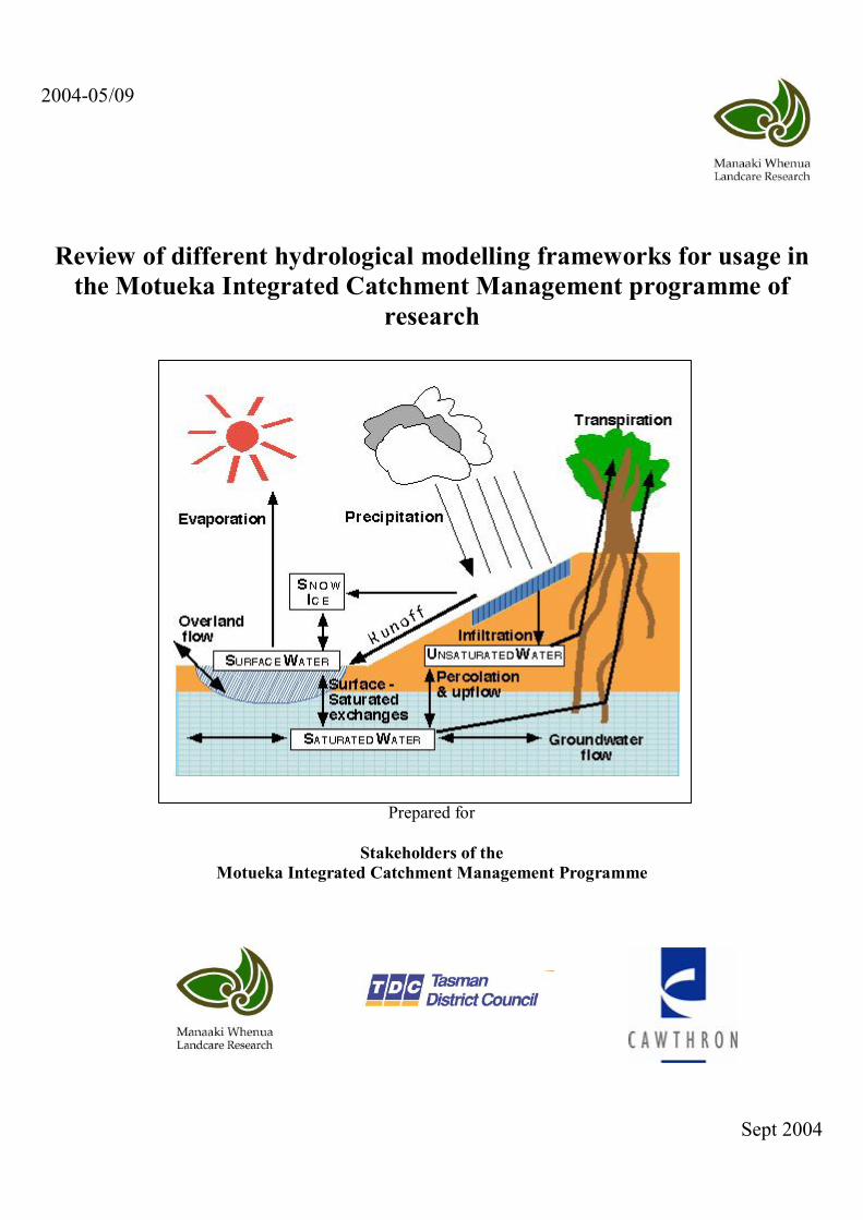
Information contained in this report may not be used without the prior consent of the client Cover Photo: Processes of the hydrological cycle frequently represented mathematically in a hydrological model.

Landcare ICM Report No. 200X­200Y/XX

Motueka Integrated Catchment Management Programme Report Series: <insert report title here>

<insert date here>

iii

PREFACE

An ongoing report series, covering components of the Motueka Integrated Catchment Management (ICM) Programme, has been initiated in order to present preliminary research findings directly to key stakeholders. The intention is that the data, with brief interpretation, can be used by managers, environmental groups and users of resources to address specific questions that may require urgent attention or may fall outside the scope of ICM research objectives. We anticipate that providing access to environmental data will foster a collaborative problem­ solving approach through the sharing of both ICM and privately collected information. Where appropriate, the information will also be presented to stakeholders through follow­up meetings designed to encourage feedback, discussion and coordination of research objectives.

4

Introduction........................................................................................................................................5

Brief overview of models reviewed .....................................................................................................5

TOPNET............................................................................................................................................6

Spatial discretisation .................................................................................................................6 Process representation ..............................................................................................................7 Potential for linkage to other models..........................................................................................8 Usable at what scale?................................................................................................................8 Other issues...............................................................................................................................8 Summary ...................................................................................................................................8

Catchment Modelling Toolkit .............................................................................................................9

Rainfall Runoff Library (RRL) ...................................................................................................9 Potential for linkage to other models........................................................................................ 10 Other issues............................................................................................................................. 10 Sediment Network (SedNet)...................................................................................................... 10 Potential for linkage to other models........................................................................................ 11 Usable at what scale?.............................................................................................................. 11 River Analysis Package (RAP) ................................................................................................. 11 Potential for linkage to other models........................................................................................ 11 Summary ................................................................................................................................. 12

SWAT.............................................................................................................................................. 13

Process representation ............................................................................................................ 13 Spatial discretisation ............................................................................................................... 14 Potential for linkage to other models........................................................................................ 15 Usable at what scale?.............................................................................................................. 15 Other issues............................................................................................................................. 15 Summary ................................................................................................................................. 15

DHVSM........................................................................................................................................... 17

Process representation ............................................................................................................ 17 Spatial discretisation ............................................................................................................... 18 Potential for linkage to other models........................................................................................ 18 Usable at what scale?.............................................................................................................. 18 Other issues............................................................................................................................. 18 Summary ................................................................................................................................. 18

PLM................................................................................................................................................. 19

Spatial discretisation ............................................................................................................... 19 Potential for linkage to other models........................................................................................ 20 Usable at what scale?.............................................................................................................. 20 Other issues............................................................................................................................. 20 Summary ................................................................................................................................. 20

Overall summary .............................................................................................................................. 21

References........................................................................................................................................ 22

5

Introduction The Integrated Catchment Management Research Programme has identified the development of a new modelling framework for investigating “catchment futures” as a priority. The modelling framework has been given the name IDEAS (Integrated Dynamic Environmental Assessment System). There is no clear understanding of what IDEAS will look like beyond a grouping of models capable of assessing cumulative effects of incremental changes in land and water management. It is clear from this that there is a requirement for a hydrological model that has capabilities of assessing land use scenarios. It is also desirable that this model links in with an Ocean­Bay circulation model to assess effects beyond the land. This paper reviews five models, or sets of models, that have some capability of performing this role and discusses their overall suitability for use within IDEAS. The review concentrates on four key areas:

• Process representation. The algorithms used within the model to represent different hydrological processes and how well these fit with available data and theoretical understanding of the processes.

• Spatial discretisation. How the model represents a river catchment and at what spatial scale are masses and fluxes transferred.

• Potential for linkage to other models. How easy would it be to either modify the model to fit in with another model (especial Ocean­Bay circulation) or to use the output data as input for another model?

• Usable (and used) at what scale. How easy would it be to set up and run the model as part of the ICM programme, and how has it been used in the past? The second question applies directly to how compatible have past runs been with using it in the Motueka.

Brief overview of models reviewed Su (1997) provides an extensive review of 60+ models available for use in hydrological analysis; it is not the intention of this paper to repeat this work. The review has chosen six models or modelling systems that are available for use and/or have been identified by researchers in the ICM programme as having potential in this field.

The models to be reviewed are: • TOPNET; a modelling system used by NIWA hydrologists in many situations

around New Zealand. • Catchment Modelling Toolkit; a modelling framework developed by the CRC

group for Hydrology in Australia. It has several models nested within a common analysis framework.

• SWAT; (SoilWater Assessment Tool) developed in the USA and applied in the Motueka using Landcare Research Reinvestment funding.

• DHVSM; (Distributed Hydrology­Vegetation­SoilModel) developed in the USA and adapted for the Motueka to look at seasonal water balance issues.

• PLM (Patuxent Landscape Model) developed in the USA as an amalgamation of an ecological and hydrological modelling approach.

• BASINS (Better Assessment Science Integrating point and Non­point Sources) is described as a “multi­purpose environmental analysis system” developed by the United States Environmental Protection Agency. It has

6

several models (including SWAT) nested within a common analysis framework.

TOPNET TOPNET is a modelling system developed by staff at NIWA for investigating water resource issues. The model started with a TOPMODEL (Beven & Kirkby, 198??) framework but has been adapted substantially so that now it can legitimately be described as a separate modelling system.

TOPMODEL was developed in the UK as a compromise between physically based distributed models, such as SHE (Systeme Hydrologique Europeen, Bathurst et al; 198??) and lumped conceptual models such as those described in the Rainfall­Runoff Library below (see page 6). The rationale for this compromise was that physically based distributed models would always be impossibly data hungry and difficult to use in a fully distributed sense. Equally, lumped distributed hydrological models could not provide the spatially distributed information required in hydrological management. The fundamental simplification the model assumes is that overland flow can be related to topography. Therefore an analysis of surface topography provides the surface runoff generating zones within a catchment. A secondary assumption from this is that subsurface flow occurs parallel to the surface. Once the area of runoff generation within a catchment is known the water balance at these points can be computed and water routed down a channel using a kinematic wave approach. TOPMODEL has been used successfully in many different countries. It’s simple structure, and success in replicating a range of hydrological flows has seen it used in both a research and operational environment. TOPNET has been used by NIWA staff for a range of scales, from the national to provide surface runoff estimates for carbon loss modelling to individual catchments for flood frequency and other hydrological analysis.

Spatial discretisation The way that TOPNET spatially represents a catchment is perhaps it's most novel feature. The starting point for any TOPNET analysis is to use a digital elevation modek (DEM) to derive a value of topographic index for a catchment. The topographic index is calculated as ln(a/tan b); where a is the area above a length of contour B. This provides a measure of how much upslope area contributes runoff to the area of contour analysed. The inherent assumption is that the greater the upslope contributing area the more runoff is produced at the particular site. This linakge between topography and runoff is verified by hillslope hollow fieldwork of Anderson & Burt (1978) and Dunne et al (1975). In TOPNET the topographic index is used to 'redistribute' runoff and soil moisture after water balance calculations are made at the sub­catchment level. Sub­catchments are derived from a DEM with user input on number and size. The sub­catchment is the basic spatial unit within TOPNET that is used for input of parameters such as land­use and soil type. The model calculates a water balance at the sub­catchment scale and then distributes the runoff and soil moisture within a sub­catchment using the topographic index as a weighting measure. The model does considerably more than just redistribute surface runoff alone, in that

7

it also calculates the soil water deficit and depth to water table, based on the topographic index.

TOPNET has a similar spatial basic representation to SWAT, (i.e. sub­catchments) however TOPNET has a significant theoretical advantage in it's linkage between topography and hydrology. The advance that TOPNET has over the original TOPMODEL is in the linkage between subcatchments and improved process representation (particularly canopy interception and evaporation).

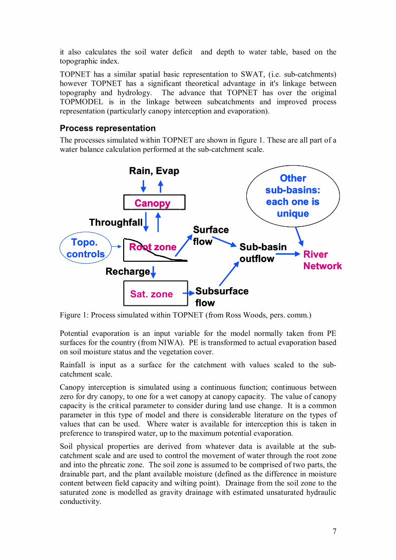
Process representation The processes simulated within TOPNET are shown in figure 1. These are all part of a water balance calculation performed at the sub­catchment scale.

Sat. zone

Rain, Evap

Subsurface flow

Recharge

Throughfall Surface flow Sub­basin

outflow River Network

Other sub­basins: each one is unique

Root zone

Canopy

Topo. controls

Sat. zone Sat. zone

Rain, Evap

Subsurface flow

Recharge

Throughfall Surface flow Sub­basin

outflow River Network

Other sub­basins: each one is unique

Other sub­basins: each one is unique

Root zone Root zone

Canopy Canopy

Topo. controls

Figure 1: Process simulated within TOPNET (from Ross Woods, pers. comm.)

Potential evaporation is an input variable for the model normally taken from PE surfaces for the country (from NIWA). PE is transformed to actual evaporation based on soil moisture status and the vegetation cover. Rainfall is input as a surface for the catchment with values scaled to the sub­ catchment scale. Canopy interception is simulated using a continuous function; continuous between zero for dry canopy, to one for a wet canopy at canopy capacity. The value of canopy capacity is the critical parameter to consider during land use change. It is a common parameter in this type of model and there is considerable literature on the types of values that can be used. Where water is available for interception this is taken in preference to transpired water, up to the maximum potential evaporation. Soil physical properties are derived from whatever data is available at the sub­ catchment scale and are used to control the movement of water through the root zone and into the phreatic zone. The soil zone is assumed to be comprised of two parts, the drainable part, and the plant available moisture (defined as the difference in moisture content between field capacity and wilting point). Drainage from the soil zone to the saturated zone is modelled as gravity drainage with estimated unsaturated hydraulic conductivity.

8

Surface and subsurface flow are aggregated at the sub­catchment level and then routed down a channel network using a kinematic wave approach to give a total hydrograph at the catchment mouth.

Potential for linkage to other models TOPNET is essentially a surface hydrology model that provides a simulation of riverflow at a point. Through the redistribution of runoff (using the topographic index approach) it is possible to get an estimate of the surface runoff at points throughout the catchment. This approach has been utilised in the past to link to other models that require this type of information. The best example of this was in the Erosion Carbon research (Landcare Research investment project finished in 2003) where the TOPNET spatially distributed output was used as input for surface erosion models to assess the amount of sediment generated at the national scale. This type could be extended to make use of the other spatially distributed information (e.g. depth to water table, soil moisture etc.) so that other erosion processes could be modelled. An example of this could be using the soil water properties to model slope failure in addition to surface erosion. The author is unaware of any other linkages made with TOPNET; for example looking at water quality and nutrient transport issues.

Usable at what scale? TOPNET has been used successfully at a range of scales from national (Erosion Carbon project) to the modelling of small catchments. It has been applied in several catchments of similar scale to the Motueka (e.g. The Grey on the West Coast; Waipoa on the East Coast). The spatial scale utilised is dependent on the input information available. TOPNET has recently been tested on a series of catchments in the USA that range in size from 800 to 2500 km 2 (Bandaragoda et al, 2004). This was part of an experiment to assess different models producing calibrated and uncalibrated outputs. TOPNET appeared to perform well in these tests (Bandaragoda et al, 2004).

Other issues The temporal scale for using TOPNET is determined by the temporal scale of inputs. For large catchments, such as the Motueka, the rainfall input is rarely at a scale finer than daily and therefore it is sensible to use the model at that scale. Where there is finer resolution rainfall data (e.g. on smaller research catchments) the model can be used with a smaller time step. This is the same as for SWAT.

Summary TOPNET is a widely accepted hydrological model that simulates a range of hydrological processes in order to produce an output hydrograph at the catchment mouth. A unique feature of TOPNET is the way that it calculates a water balance at the sub­catchment scale and then redistributes the runoff within the sub­catchment using a topographic index as a weighting measure. This provides an estimate of the surface runoff (and other soil water properties) at points throughout the catchment.

9

Catchment Modelling Toolkit The Co­operative Research Centre (CRC) for Catchment Hydrology in Australia has produced a series of models in their catchment modelling toolkit. These models are freely available and can be downloaded from the web after a simple registration with the CRC. At present there are eight modelling platforms available within the catchment modelling toolkit.

• CHUTE – a spreadsheet programme for the design of rock chutes. These are used in rivers and channels to stabilise erosion (similar to rip­rap).

• MUSIC – a decision support system for evaluating urban storm water design. • RAP – models river condition and river restoration design. • RRL – is the Rainfall Runoff Library that contains five different models that

can be used to simulate runoff at a range of different scales. • SCL – is a library of stochastic models for generating climatic data (e.g.

rainfall and potential evapotranspiration) at a site. • SedNet – constructs sediment budgets for river networks. • TIME – is not a model as such but is a model development platform for

creating and testing new models. • TREND – a time series analysis package designed specifically for

hydrological data. Of these, the three that appear to have direct applicability to the Motueka ICM project are RRL; SedNet and RAP. These are considered separately here.

Rainfall Runoff Library (RRL) The models in the RRL are designed to simulate catchment runoff using daily rainfall and evapotranspiration. The actual model chosen for use in a particular situation is dependent on the data available to parameterise it and the detail required in the application. The models currently available are all spatially simplistic. They use a simple system of a single unit or can be linked as a series of sub­catchment but cannot be used in a truly distributed fashion. The models are:

• AWBM – is a lumped conceptual water balance model derived from the work of Boughton. It has many similarities to the water balance model developed at Landcare Research for the SMF funded project on effects of tall vegetation. Each catchment is treated as a single unit; there are three surface stores which produce surface runoff and a separate baseflow store. The model operates at a daily time step and require some knowledge of streamflows in order to calibrate it. One oddity of AWBM is that it requires actual evapotranspiration as input; as opposed to potential evapotranspiration that the other models in the toolkit require.

• SACRAMENTO – is a water balance model with more detail than the AWBM. It is derived from North America and has been widely used for simulating surface flows. The emphasis within the model is on simulating different types of runoff (surface; throughflow and baseflow) from the surface layers.

• SIMHYD – is a lumped conceptual model that includes canopy process representation

• SMAR – concentrates on soil moisture accounting with a separate runoff routing routine. It is another lumped conceptual model.

10

• TANK – is the simplest of the models in the RRL. It consists of four “tanks” that represent surface stores. The amount of water in each tank is affects the amount of evaporation, infiltration and runoff. The tank storage is calculated in order so that conceptually it is moving down a soil/bedrock profile.

The difference between these models is in the process representation. Each is essentially as set of stores but different models have different levels of sophistication in how those stores are defined. Equally the parameters have different levels of physical meaning. SMAR and SIMHYD provide the greatest level of sophistication.

The models are in a PC framework that provides outputs including standard hydrological analyses (e.g. flow duration curves). Each model has a set of default values given with it. In addition to the models there are range of tools available through the library that can be used for calibration, validation and optimisation.

Potential for linkage to other models Each of these models simulates runoff at the catchment (or possibly sub­catchment) scale. This information can be linked to other models although the lack of spatial distribution makes it difficult to see how they can be used for investigation issues of cumulative effect within a catchment.

Other issues The real advance provided by the RRL is not in the models used but in putting several commonly used models (certainly commonly used in engineering hydrology) into a single framework for use on a desktop PC. By having them all together the practitioner can try different models for the same application and has a very good set of optimisation tool available for use with the different models.

Sediment Network (SedNet) SedNet is a model designed to provide sediment budgets for river networks. It operates at a mean annual time scale so is not designed to provide event­based assessment of sediment fluxes from a catchment; nor is it designed to investigate year­ on­year variation in sediment flux. However, SedNet does provide a means of investigating management options on mean annual sediment yield from a catchment.

SedNet operates as a series of sub­catchments (referred to as links) within a stream network. Sediment budgets are calculated for each link (effectively the mouth of each sub­catchment) as an accumulation of loss from the sources and stores within each sub­catchment. The size and extent of sources (gullies, hillslopes; river banks) and sinks (floodplains; dams, lakes, wetlands) are defined using GIS information (using an ARC­INFO interface). These are derived from DEM data and other spatial information such as extent and type of riparian vegetation. Parameters controlling flux movement (channel roughness, sediment density and particle size, hillslope delivery ratio) are required for each sub­catchment. The movement of sediment between links, along the stream networks, is controlled by hydrological information. Because the model operates at a mean annual time scale the hydrological information required is generalised rather than a specific time series. The type of information required is: mean annual flow; a separate measure of daily flow variability; and bankfull discharge. This information is input for the whole catchment and regionalised within using relationships to rainfall variation within the catchment and runoff coefficients.

11

Once the input parameters have been set the model operates a series of budgets within the stream network. These budgets account for: bedload; bank erosion (modelled in a relationship to stream power and riparian vegetation); suspended sediment; floodplain and reservoir deposition.

Potential for linkage to other models The operational time­scale of the model means that it cannot be linked at the event­ scale. This seriously limits its use within a modelling system aimed at assessing dynamic cumulative effect.

The version of SedNet currently available concentrates solely on sediment fluxes, however the CRC ststes on it’s website that a new version currently being developed will included nutrient budgets (phosphorus and nitrogen). As with the sediment flux this will be restricted to mean annual loads. According to the SedNet user guide the new version:

“considers the physical and not the biological stores of nutrients, and is primarily concerned with the physical transport processes. It does however consider denitrification and phosphorus absorption­desorption.” (SedNet User Guide, page 52).

This type of information could be used for assessing impacts of local management options.

Usable at what scale? SedNet has been designed in the Australian context for large­scale regional application. The user guide states:

“the most appropriate scale for SedNet modelling is across large regions (10 3 – 10 6 km 2 ), and the model; outputs should be interpreted as indicating patterns across the region, rather than accurate estimates of sediment supply in a particular sub­catchment.” (SedNet User Guide, page 2).

The Motueka catchment comes in at the bottom end of this scale (2x10 3 km 2 ).

River Analysis Package (RAP) The River Analysis Package provides quantitative tools for in­stream river management and assessment. The package is split into two separate modules:

• Hydraulic analysis – constructs a 1­dimensional hydraulic model of a river reach. This can be used to determine ecologic thresholds based on hydraulic parameters.

• Time series analysis – provides a time series package, with graphical outputs for rapid assessment of time series hydrological data.

Of these two modules the hydraulic analysis is the most useful in a modelling sense. Input data required are channel cross sections (n.b. as the model is 1­dimensional it takes a single cross section per reach) and channel roughness. This data can then be combined with time series data to produce a time series of key attribute such as local depth or wetted perimeter. The hydraulic model is simple in design and use and therefore cannot be used in complex problems. It could be used for looking at particular sites on the Motueka but not continuous reaches or the whole river channel.

Potential for linkage to other models The main linkage that could be foreseen is another hydrological model providing time series data for use in RAP; rather than the other way around. Essentially RAP

12

provides a simple analysis tool to explore scenarios that may have been generated elsewhere.

Summary The catchment modelling toolkit provides a variety of models for use in problem solving. Three of these have particular relevance to the ICM Motueka project. Individually these models have various strengths and weaknesses. Overall the strength of the catchment modelling toolkit is in bringing the different models together so that they can run on a common computer platform with similar looking output.

13

SWAT The Soil Water Assessment Tool (SWAT) has been developed in the USA as catchment scale model to:

“predict the impact of land management practices on water, sediment and agricultural chemical yields in large complex watersheds with varying soils, land use and management conditions over a long period of time” (SWAT User Manual, page 1).

If the model were successful in achieving this then it would appear to be the perfect tool for use in IDEAS. The model is derived from several well­known predecessors:

• SWRRB – Simulator for Water Resources in Rural Basins provides th basic hydrology

• CREAMS – Chemicals, Runoff and Erosion from Agricultural Management Systems for the nutrient and some sediment transport.

• GLEAMS – Groundwater Loading Effects on Agricultural Management Systems for the groundwater quality component.

• EPIC – Erosion­Productivity Impact Calculator for the link between erosion; sediment transport and nutrient loss/gain.

All of these are physically based models in their own right; SWAT combines them into a distributed framework that operates at the catchment scale. The majority of, although not all, SWAT applications have been in smaller catchments than the Motueka. Where the catchments have been larger they tend not have been in mountainous or such diverse landscapes.

There are three interesting features of SWAT: 1. There is multiple process representation, allowing the user to choose the most

appropriate for the particular application. 2. It combines simulated hydrology, sediment and nutrient transport in one

model. 3. The spatial representation within the model.

Process representation There is not enough room in this document to describe all the process representations available in SWAT. One of the strong features of SWAT is that there are normally several different process representations available for all the major hydrological processes that could be represented. An example of this can be seen in the representation of evapotranspiration (ET). There are three available routines for this:

• Penman­Monteith: simulates ET from measurements of net radiation, humidity, air temperature, windspeed above a canopy; atmospheric pressure; and canopy resistance (or stomatal resistance).

• Priestly­Taylor: simulates potential ET as a simplification of the Penman equation. It applies at a large scale and consequently needs less data across a catchment.

• Hargreaves: the simplest method that bases potential ET on air temperature across the catchment.

It is up to the user to decide which is the most applicable for a particular situation. In the simulations for the Motueka the Hargreaves method has been used because there is insufficient data for the other two methods and tests showed that it was an adequate

14

representation for potential ET for a short period where it could be tested against Penman­Monteith at a particular point.

At the soil surface, infiltration can be represented using the Green­Ampt equation, after rainfall has been adjusted for canopy interception using canopy interception capacity. Another method simulating, and that used in the Motueka simulation so far, uses a curve number approach. This is a common approach in the USA, which gives the amount of surface runoff generated (and consequently that which infiltrates) for a given rainfall. Essentially this simplifies the canopy interception and rainfall­runoff relationship into a simple curve. A different curve is chosen for each vegetation and soil type. The consideration of land use change comes through changing the particular curves used. One of the difficulties in using SWAT in the Motueka has been finding the right curve types for the conditions; the standard curves are derived from data in the American mid­west. In most other ways SWAT operates as a physically based hydrological model. Processes such as nutrient cycling within a stream; phosphorus absorption and desorption have simulation routines, the difficulty is in obtaining the necessary data to run the routines. Plant growth can be simulated with both seasonal and yearly variation. Water is routed through the channel network using a kinematic wave approach. Sediment generation comes from the Modified Universal Soil Loss Equation (MUSLE). This uses the amount of surface runoff to simulate erosion and sediment yield. This limits erosion to surface processes; large­scale processes such as landsliding and bank erosion are ignored. This is a major limitation on the use of SWAT for an environment such as the Motueka where sediment delivery to the stream bank through landsliding is a known occurrence.

Spatial discretisation The most novel aspect of SWAT is in the spatial representation. A catchment is first split into sub­catchments (referred to as sub­basins in the SWAT literature) based on data from a Digital Elevation Model (DEM). The user can set the number of sub­ basins; the chosen number is normally a compromise between computational efficiency and topographic variability. The sub­basin is the fundamental spatial unit within a SWAT simulation. In the Motueka work so far the catchment has been split into 491 sub­basins (giving an average area of 4.5 km 2 ).

Each sub­basin has a separate rainfall input; but it is assumed that the rainfall does not vary within each sub­basin. In the original version of SWAT the rainfall is assumed to come from the nearest rain gauge. This has been changed so that a new rainfall surface is generated based on the annual rainfall distribution and the spatial distribution of gauges. This was a separate pre­processing routine written by Wenzhi Cao for the Motueka.

Within each sub­basin the model produces “hydrological response units” (HRU) based on the land cover, and soil type. The user also specifies the number of HRU per sub­basin; the manual recommends between 1­10 per sub­basin. An HRU is the fundamental unit at which hydrological response occurs but there is no spatial element attached to an individual HRU. If a sub­basin has 10 HRU then it accumulates the flow (or nutrients) from each HRU, within a timestep, it has no way of understanding whether one HRU is closer to the sub­basin exit than another.

15

In summary the sub­basin is the fundamental spatial unit within SWAT and the HRU is the fundamental unit for calculation (e.g. water balance and/or nutrient balance).

Potential for linkage to other models The compiled code for SWAT is down loadable from a website and therefore available for use immediately. This means that we cannot alter the source code to link directly with another model (e.g. ocean­bay circulation model). However the output from the model can be linked as the input for another. In the same way that Wenzhi Cao has written a pre­processing routine for precipitation in SWAT it is possible to write a post­processing routine to match the input of a secondary model.

The fact that SWAT has nutrient, pesticide and sediment modelling capabilities within its current structure means that there is less requirement to link to other models. There are particular limitations in the sediment modelling capabilities that make it difficult to see it playing a meaningful role in sediment modelling.

Usable at what scale? SWAT has been tested at the Motueka scale and found to be an adequate simulator of surface hydrology. There is a paper currently submitted to Hydrological Processes which shows the multiple calibration and validation criteria used to do this. The major limitation in using a model like SWAT at the scale of the Motueka catchment is in obtaining the necessary input variables and parameters. Of particular concern is the poor coverage of soil properties and the difficulties in getting a good rainfall coverage.

It is clear from using SWAT that it has developed up from a small catchment model into something used for larger scales. The most obvious example of this is in the rainfall routine where each sub­basin looks for the closest rain gauge to give a daily total. This would work adequately at a small scale with little variation but becomes problematic at the large scale, and high rainfall variability, of the Motueka. The moving from small scale to large is a common problem in hydrology that has not been adequately addressed. In taking a model such as SWAT up in scale the inherent assumption is made that the hydrological relationships are scale independent. This is often not true and is subsequently ignored.

Other issues At present SWAT operates on a daily timestep. There is no computational reason why it couldn’t operate on a shorter timestep however in a catchment the size of the Motueka this would be unwise for two reasons. First, the main hydrological input (rainfall) is recorded at a daily timestep so there is insufficient data to run it at a shorter timestep. Second, the assumption is made that water (and nutrients/sediment etc) move through a sub­basin within a single timestep. With an average sub­basin size of 4.5 km 2 the reconfigured timestep would have to take into account whether water could move from slope to sub­basin mouth within the shorter timestep.

Summary SWAT provides an all­encompassing model for hydrology and nutrients at a daily timestep. It has been shown to adequately reproduce surface hydrology in the Motueka and is currently being worked on the reproduce nutrient data. The model is complex and has huge data requirements, few of which can be adequately met. It has taken two years to set up and run in the Motueka, which suggests that it is not easy to

16

transfer between sites. Given the effort that has gone into calibration and validation so far it would be foolish to give it up for another similar model but careful consideration needs to be given as to whether it is really usable by land resource managers. SWAT can produce outputs based on modelled scenarios that can then be captured in the CD­ROM. This is of use to land resource managers but it is difficult to see SWAT running separately on managers’ desktops.

17

DHVSM Wigmosta et al. (1994) developed the distributed hydrology­vegetation­soil model (DHVSM) that simulates most components of the hydrological cycle, at grid points throughout a catchment. Recently Robbie Andrew and John Dymond have developed a version of DHVSM to provide seasonal water balances for the Motueka catchment in a spatially distributed manner (Andrew & Dymond, in prep). This is the version of model described here.

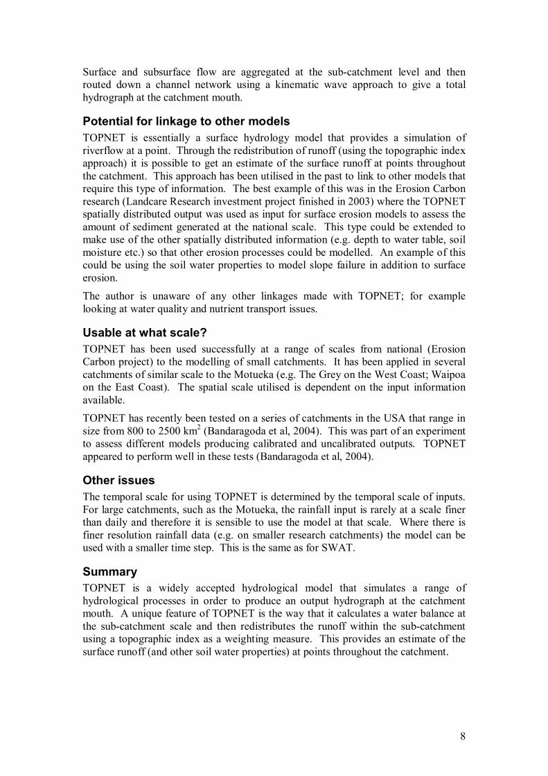
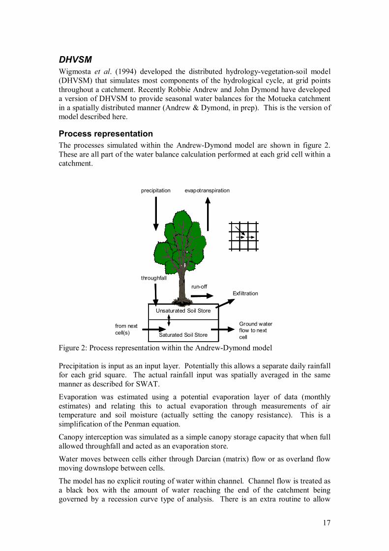
Process representation The processes simulated within the Andrew­Dymond model are shown in figure 2. These are all part of the water balance calculation performed at each grid cell within a catchment.

precipitation evapotranspiration

throughfall

from next cell(s)

Unsaturated Soil Store

Saturated Soil Store

run­off

Ground water flow to next cell

Exfiltration

Figure 2: Process representation within the Andrew­Dymond model

Precipitation is input as an input layer. Potentially this allows a separate daily rainfall for each grid square. The actual rainfall input was spatially averaged in the same manner as described for SWAT. Evaporation was estimated using a potential evaporation layer of data (monthly estimates) and relating this to actual evaporation through measurements of air temperature and soil moisture (actually setting the canopy resistance). This is a simplification of the Penman equation. Canopy interception was simulated as a simple canopy storage capacity that when full allowed throughfall and acted as an evaporation store. Water moves between cells either through Darcian (matrix) flow or as overland flow moving downslope between cells. The model has no explicit routing of water within channel. Channel flow is treated as a black box with the amount of water reaching the end of the catchment being governed by a recession curve type of analysis. There is an extra routine to allow

18

deep storage of water and slow release into the channel; effectively simulating groundwater released baseflow.

Spatial discretisation The current Andrew­Dymond model computes the water balance on a 25mx25m grid cell basis (see figure 2). This has been used to simulate river flows in the Motueka at Woodstock (Andrew & Dymond, in prep).

Potential for linkage to other models In the same manner as any of the other hydrological models reviewed here the output from the Andrew­Dymond model can be used as input for other model tools. The lack of explicit surface routing routines make it impossible to model in­stream processes. Although the model is able to reproduce hydrographs at Woodstock there has been no internal validation of model output. As an example it cannot be said whether the model is good or bad at predicting the spatial variability in soil moisture; a key variable in sediment and nutrient movement. Overall, there is no reason why it cannot be linked to other models but it provides no particular advantages over other models (e.g. TOPNET and SWAT) and has not been fully tested.

Usable at what scale? The Andrew­Dymond model was developed exclusively for use in the Motueka and has a flexible grid­based network that means it can easily be adjusted for different scales.

Other issues As used so far the Andrew­Dymond model has been calibrated to hydrographs using saturated hydraulic conductivity (Ksat) as the sole adjusted parameter. The calibrated values for Ksat are far higher than would normally be expected from field and laboratory measurements. However the model is able to reproduce total catchment hydrographs using these values, which raises a problem of equifinality. It seems likely that the “correct hydrograph” result is a sum of many different processes and it is likely that each internal processes is not necessarily correct. The problem of equifinality is not limited to the Andrew­Dymond model; many others suffer from the same problem, something that is not always made explicit in the literature.

Summary The Andrew­Dymond model is able to simulate Motueka hydrographs but there are limitations in its usage for further modelling. These limitations hinge around the simplifications in the model structure (no explicit channel routing; simplified evaporation routine) and the lack of full model testing.

19

PLM The Patuxent landscape model (PLM) is described as a:

“…spatially explicit, multiscale, process­based model designed to serve as a tool in a systematic analysis of the interactions among the physical and biological dynamics of the watershed, conditioned on socioeconomic behaviour in the region” (Costanza, et al. 2002, page 206).

This description makes it sound ideal for use in IDEAS! The Patuxent watershed (2352 km 2 ) in Maryland, USA is of similar size to the Motueka (2200 km 2 ) with diverse and changing land use although not as diverse in topography and rainfall.

The PLM operates on a grid cell network with what is referred to as a general ecocsystem model (GEM) operating at each cell. The GEM is calculating flux balances in each cell and transferring mass between cells. The GEM is made of three “modules”:

• Hydrology (precipitation, evapotranspiratiopn, infiltration and percolation); • Nutrients (N & P inputs and outputs, with cycling); • Plants (biomass accumulation)

Within each cell the hydrology, nutrient and plant status is simulated within a time step (daily) and then a separate routine calculates the fluxes between cells. The actual routines used to simulate these processes are not described in Costanza et al (2002), it is assumed that have a physical basis. The processes described are similar to those covered by SWAT.

PLM treats channel and overland flow in a singular manner. It assumed that all overland flow reaches some kind of channel within a cell and then is treated as channel flow using a kinematic wave approach to move this water between cells. The real innovation in the PLM lies in its linkage to what is termed the Economic Land­Use Conversion (ELUC) model. This operates quite separately and provides an estimate of likely land­use change for the particular part of a catchment. ELUC is empirically based (i.e. based on known measurements of land use change) and uses land value and proximity to different infrastructure services (e.g. roads, sewerage etc.) as dependent variables in coming up with a likelihood f land use change at a point. The land use change considered is conversion from forest or agriculture to urban. Once likelihoods had been generated this was compared to different urban growth scenarios to predict where the growth might occur and therefore what impacts PLM predicts the changes might make.

Spatial discretisation The grid pattern used in PLM was varied according to the overall scale of modelling undertaken. Three scales were trialled (23, 940 and 2352 km 2 ). When operating at the smallest scale the grid size was 200m x 200m but for the total catchment this was reduced to 1km x 1km for the ecological modules. Considerable variation was found in the hydrological accuracy when the model was scaled up, suggesting that there were scale factors unaccounted for in the model structure. The use of multiple scales within the model is novel.

20

Potential for linkage to other models PLM has exactly the same potential for linkage to other models as the others considered here. The fact that it has nutrient dynamics already simulated means there is little need to link with other water quality models in the land­freshwater arena.

Usable at what scale? PLM has been developed at a scale comparable to the Motueka. When used at the full Patuxent scale simplifications in structure were made which would make it difficult to represent the large ecological and landscape diversity within the Motueka.

Other issues The model is operating at a daily timestep.

Summary The PLM combines hydrology, nutrient movement and plant growth in a grid­based network. In the description given by Costanza et al (2002) it is linked to a separate land use change simulator to consider impacts of urban growth in the catchment. This type of land use change predictor could equally be used with any of the models described here.

21

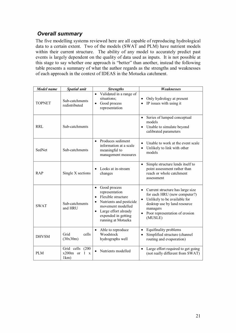
Overall summary The five modelling systems reviewed here are all capable of reproducing hydrological data to a certain extent. Two of the models (SWAT and PLM) have nutrient models within their current structure. The ability of any model to accurately predict past events is largely dependent on the quality of data used as inputs. It is not possible at this stage to say whether one approach is “better” than another, instead the following table presents a summary of what the author regards as the strengths and weaknesses of each approach in the context of IDEAS in the Motueka catchment.

Model name Spatial unit Strengths Weaknesses

TOPNET Sub­catchments redistributed

• Validated in a range of situations;

• Good process representation

• Only hydrology at present • IP issues with using it

RRL Sub­catchments

• Series of lumped conceptual models

• Unable to simulate beyond calibrated parameters

SedNet Sub­catchments

• Produces sediment information at a scale meaningful to management measures

• Unable to work at the event scale • Unlikely to link with other

models

RAP Single X sections • Looks at in­stream

changes

• Simple structure lends itself to point assessment rather than reach or whole catchment assessment

SWAT Sub­catchments and HRU

• Good process representation

• Flexible structure • Nutrients and pesticide

movement modelled • Large effort already

expended in getting running at Motueka

• Current structure has large size for each HRU (new computer?)

• Unlikely to be available for desktop use by land resource managers

• Poor representation of erosion (MUSLE)

DHVSM Grid cells (30x30m)

• Able to reproduce Woodstock hydrographs well

• Equifinality problems • Simplified structure (channel

routing and evaporation)

PLM Grid cells (200 x200m or 1 x 1km)

• Nutrients modelled • Large effort required to get going (not really different from SWAT)

22

References

Anderson, M.G. and Burt, T.P. (1978) The role of topography in controlling throughflow generation. Earth Surface Processes 3:331­334

Andrew, R.M. & Dymond, J.R. (in prep) A distributed model of water balance in the Motueka catchment, New Zealand. Submitted to Journal of Hydrology (NZ) 2004.

Bandaragoda, C., Tarboton, D.G., & Woods, R. (2004) Application of TOPNET in the distributed model intercomparison project. Journal of Hydrology 298:178­ 201.

Costanza, R., Voinov, A., Boumans, R., Maxwell, T., Villa, T., Wainger, L. & Voinove, H. (2002) Integrated Ecological Economic modelling of the Patuxent River watershed, Maryland. Ecological Monographs 72(2):203­231.

Dunne, T. Moore, T.R. & Taylor, C.H.. (1975) Recognition and prediction of runoff­ producing zones in humid regions. Hydrological Science Bulletin 20:305­326.

Su, N. (1997) A survey of computer models used in hydrological analysis and data management. Landcare Research discussion paper.

Wigmosta, M.S.; Vail, L.W.; Lettenmaier, D.P. 1994: A distributed hydrology­ vegetation model for complex terrain. Water Resources Research 30: 1665– 1679