307
2006 Stream EC trends for inland New South Wales

2006 Stream EC trends for inland New South Wales

Acknowledgments
Dr. Greg Summerell for advice on the use of catchment characteristics. Mark Mitchell for advice on the hydrogeology of the Murrumbidgee Valley. Geoff Beale for general advice throughout the project.
The previous work on the application of Generalised Additive Models to trend estimation by Richard Morton is acknowledged. Hugh Jones (DECC) and Dr Amrit Kathuria (since moved to work for NSW DPI) gave of their time and statistical expertise via discussions on formulating the key statistical steps and methodology for this analysis, and its implementation within the S-PLUS software package. Prepared by: Frank Harvey, Wagga Wagga Research Centre Terry Koen, Cowra Research Centre Michelle L Miller, Wagga Wagga Research Centre Sarah J McGeoch, Wagga Wagga Research Centre Published by: Department of Environment and Climate Change NSW 59–61 Goulburn Street PO Box A290 Sydney South 1232
Phone: (02) 9995 5000 (switchboard) Phone: 131 555 (environment information and publications requests) Phone: 1300 361 967 (national parks information and publications requests) Fax: (02) 9995 5999 TTY: (02) 9211 4723
Email: [email protected] Website: www.environment.nsw.gov.au In April 2007 the Department of Natural Resources became part of the Department of Environment and Climate Change NSW. This material may be reproduced in whole or in part, provided the meaning is unchanged and the source is acknowledged. ISBN 978 1 74122 870 0 DECC 2009/55 February 2009
While every reasonable effort has been made to ensure that this document is correct at the time of printing, the State of New South Wales, its agents and employees, disclaim any and all liability to any person in respect of anything or the consequences of anything done or omitted to be done in reliance upon the whole or any part of this document.

Contents
Abstract..............................................................................................................................................9
Foreword..........................................................................................................................................10
1 Introduction.............................................................................................................................1 1.1 Previous work..............................................................................................................1 1.2 General approach of this report...................................................................................2
2 Data ........................................................................................................................................6 2.1 Background .................................................................................................................6 2.2 Historical EC dataset—(late 1960s to early 1990s).....................................................7 2.3 Recent EC dataset (1993 to present) ..........................................................................7 2.4 Time-series..................................................................................................................8 2.5 Amalgamation of various EC data systems.................................................................8 2.6 Groundwater data........................................................................................................9 2.7 Catchment characteristics ...........................................................................................9
3 Input Dataset ........................................................................................................................11 3.1 Final preparation of data............................................................................................11 3.2 Characteristics of input data ......................................................................................11
4 Statistical Methodology.........................................................................................................16 4.1 Aim ............................................................................................................................16 4.2 Background ...............................................................................................................16 4.3 Formulation of the model...........................................................................................16 4.4 Graphical insight into model structure .......................................................................18 4.5 Interpretation of analysis ...........................................................................................23 4.6 Correlated residual terms ..........................................................................................24 4.7 Model hierarchy.........................................................................................................25 4.8 Trend indicators.........................................................................................................26 4.9 Comparison with catchment characteristics ..............................................................27 4.10 Groundwater pilot study.............................................................................................27
5 Results..................................................................................................................................28 5.1 Performance of models .............................................................................................28 5.2 EC trend indicators ....................................................................................................41 5.3 Catchment characteristics .........................................................................................51 5.4 Model performance and catchment characteristics ...................................................57
6 Preliminary Catchment Groups ............................................................................................59 6.1 Categorisation (southern valleys) ..............................................................................60 6.2 Catchment characteristics as an explanation of trend...............................................75
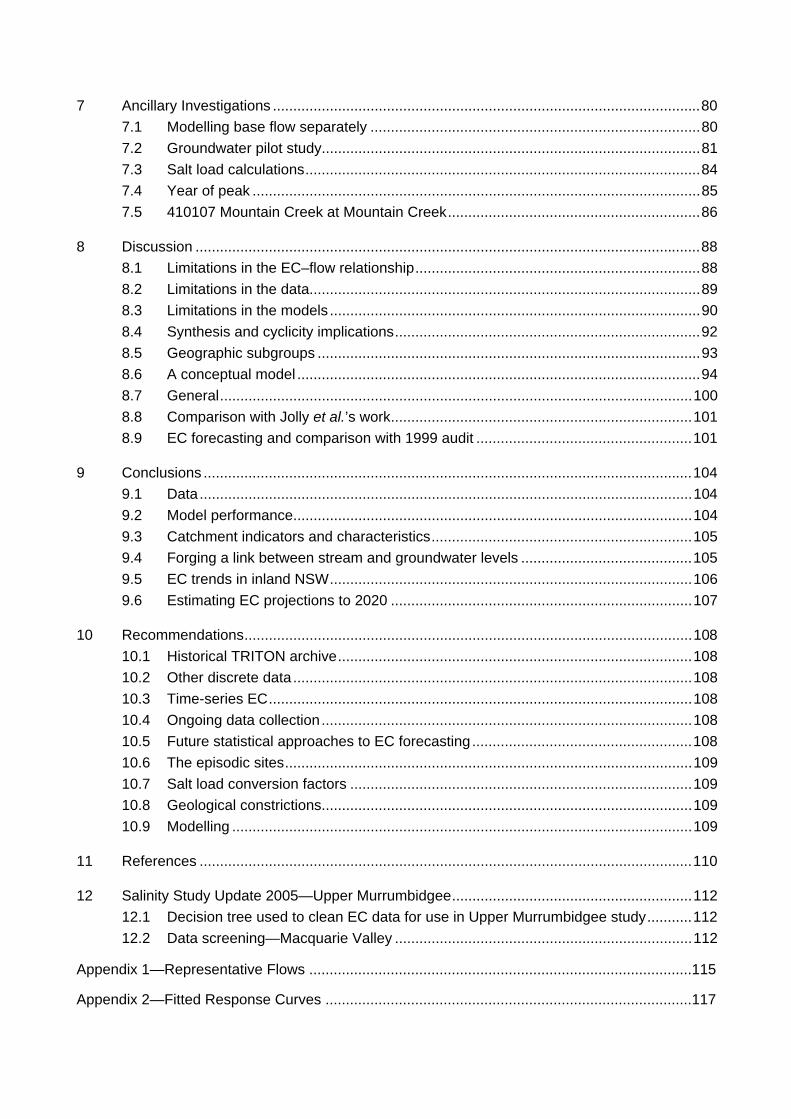
7 Ancillary Investigations .........................................................................................................80 7.1 Modelling base flow separately .................................................................................80 7.2 Groundwater pilot study.............................................................................................81 7.3 Salt load calculations.................................................................................................84 7.4 Year of peak ..............................................................................................................85 7.5 410107 Mountain Creek at Mountain Creek..............................................................86
8 Discussion ............................................................................................................................88 8.1 Limitations in the EC–flow relationship......................................................................88 8.2 Limitations in the data................................................................................................89 8.3 Limitations in the models ...........................................................................................90 8.4 Synthesis and cyclicity implications...........................................................................92 8.5 Geographic subgroups ..............................................................................................93 8.6 A conceptual model ...................................................................................................94 8.7 General....................................................................................................................100 8.8 Comparison with Jolly et al.’s work..........................................................................101 8.9 EC forecasting and comparison with 1999 audit .....................................................101
9 Conclusions ........................................................................................................................104 9.1 Data.........................................................................................................................104 9.2 Model performance..................................................................................................104 9.3 Catchment indicators and characteristics................................................................105 9.4 Forging a link between stream and groundwater levels ..........................................105 9.5 EC trends in inland NSW.........................................................................................106 9.6 Estimating EC projections to 2020 ..........................................................................107
10 Recommendations..............................................................................................................108 10.1 Historical TRITON archive.......................................................................................108 10.2 Other discrete data ..................................................................................................108 10.3 Time-series EC........................................................................................................108 10.4 Ongoing data collection...........................................................................................108 10.5 Future statistical approaches to EC forecasting ......................................................108 10.6 The episodic sites....................................................................................................109 10.7 Salt load conversion factors ....................................................................................109 10.8 Geological constrictions...........................................................................................109 10.9 Modelling .................................................................................................................109
11 References .........................................................................................................................110
12 Salinity Study Update 2005—Upper Murrumbidgee...........................................................112 12.1 Decision tree used to clean EC data for use in Upper Murrumbidgee study...........112 12.2 Data screening—Macquarie Valley .........................................................................112
Appendix 1—Representative Flows ..............................................................................................115
Appendix 2—Fitted Response Curves ..........................................................................................117

Appendix 3—Base Flow Separation .............................................................................................210
Appendix 4—Groundwater pilot study ..........................................................................................220
Appendix 5—Forecasting EC for 2020 .........................................................................................225
Appendix 6—S-PLUS Script Input File .........................................................................................227
Appendix 7—S-PLUS Script Output File ......................................................................................234
Appendix 8—Derivation of {100 × (eη – 1)} ..................................................................................273
Annexure A—Aspects of Archived Electrical Conductivity Data in TRITON ...............................277
Figures Figure 1. NSW map showing the 8 valleys investigated in this report. ..............................................3 Figure 2. The 49 catchments that comprise the study sites in the southern half of NSW. ................4 Figure 3. The 43 catchments that comprise the study sites in the northern half of NSW. .................5 Figure 4. Schematic diagram of discrete sample collection program. ...............................................6 Figure 5. Distribution of highest sampled flow as flow-weighted percentiles...................................15 Figure 6. Comparison of polynomial and smoothing spline curves on irregularly shaped data.......17 Figure 7. Differing degrees of linearity in logeEC and logeflow relationships. ..................................19 Figure 8. Fitting a spline function of logeflow to logeEC. ..................................................................20 Figure 9. Calculation of ‘EC adjusted for flow’. ................................................................................20 Figure 10. Modelling seasonality within EC trends. .........................................................................21 Figure 11. Calculation of EC adjusted for flow and seasonality.......................................................21 Figure 12. Differing degrees of curvature of adjusted EC over time................................................22 Figure 13. Flow chart of hierarchical model sequence. ...................................................................26 Figure 14. Map showing performance of Model 3, southern NSW. .................................................31 Figure 15. Map showing performance of Model 3, northern NSW...................................................32 Figure 16. Model 3, distribution of R2 across NSW..........................................................................33 Figure 17. Map showing performance of Model 5, southern NSW. .................................................34 Figure 18. Map showing performance of Model 5, northern NSW...................................................35 Figure 19. Model 5, distribution of R2 across NSW..........................................................................36 Figure 20. Map showing performance of Model 7, southern half of NSW. ......................................37 Figure 21. Map showing performance of Model 7, northern half of NSW........................................38 Figure 22. Model 7, distribution of R2 across NSW..........................................................................39 Figure 23. Plot of Model 3 R2 vs Model 7 final R2 in all central and northern valleys. .....................40 Figure 24. Plot of Model 3 R2 vs Model 7 final R2 in Murray–Murrumbidgee–Lachlan valleys. .......41 Figure 25. Matrix plot of 3 measures of trend. .................................................................................46 Figure 26. Catchment characteristics matrix plot.............................................................................52 Figure 27. Highlighting the Snowy subgroup rainfall and elevation. ................................................53
Figure 28. Mean EC envelope. ........................................................................................................57 Figure 29. Model performance and catchment characteristics (excl. Snowy group). ......................58 Figure 30. Subgroups in southern NSW. .........................................................................................59 Figure 31. Typical GAM curves for Snowy and Upper Murrumbidgee subgroups...........................61 Figure 32. Typical GAM curves for Lachlan Mountains and Lachlan Rising subgroups..................64 Figure 33. Typical GAM curves for Southern Trending subgroup. ..................................................65 Figure 34. Typical GAM curves for the Bogan and Upper Macquarie subgroups. ..........................69 Figure 35. Typical GAM curves for the Warrumbungle and Central Macquarie subgroups. ...........71 Figure 36. Typical GAM curves for the 3 northern valleys...............................................................74 Figure 37. Catchment groups relative to mean annual rainfall and elevation..................................76 Figure 38. Catchment groups relative to linear trend and gauge elevation. ....................................76 Figure 39. Catchment groups relative to linear trend and hypsometric integral. .............................77 Figure 40. Catchment groups relative to linear trend and mean annual rainfall. .............................78 Figure 41. Catchment groups relative to linear trend and catchment slope. ...................................78 Figure 42. Catchment groups relative to percentage of cycle and hypsometric integral. ................79 Figure 43. Comparison of all data with base flow data only. ...........................................................80 Figure 44. Geomorphology near Breeza. ........................................................................................84 Figure 45. Elevation v year of GAM peak. .......................................................................................86 Figure 46. 410107 Mountain Creek at Mountain Creek and environs. ............................................87 Figure 47. Adequate spline fit. .........................................................................................................91 Figure 48. Spline not fitting flow extremes.......................................................................................92 Figure 49. Conceptual diagram in Section 8.5.2..............................................................................94 Figure 50. Examples of episodic behaviour in Jolly et al.’s Zone 1. ................................................96 Figure 51. The episodic catchments (‘E’) and catchments of interest (pink). ..................................97 Figure 52. Zones in the southern part of NSW. ...............................................................................99

Tables Table 1. Flow duration data (ML/d) showing the extent to which EC sampling is
representative of flows..........................................................................................................12 Table 2. Data set statistics and coefficients of determination (R2) for various models. ...................29 Table 3. Summary statistics from fitting the GAM shown as Equation 1. ........................................43 Table 4. Trend statistics fitting the GAM shown as Equation 1. ......................................................48 Table 5. Trend, cyclicity and catchment characteristics. .................................................................54 Table 6. Comparison of linear coefficient for all data and base flow data. ......................................81 Table 7. Impact on R2 of including groundwater component. ..........................................................82 Table 8. Comparison with Jolly et al. (1997) results for 7 common sites.......................................101 Table 9. Comparison between this study and 1999 Audit for 2020/1998 EC ratios. .....................103

Abstract
This study was undertaken to quantify electrical conductivity (EC) trends in 92 river tributaries in inland NSW. The statistical approach used is a variation of the methods detailed in Jolly et al. (1997) and Morton (2002), and examined a number of models of varying complexity which attempted to quantify EC trend. Most successful was a Generalised Additive Model that proposed the natural logarithm of EC as a function of the combined effects of a spline function of the logarithm of instantaneous flow, a seasonality term within years and a spline function of time.
Two trend indicators were used: a linear trend (on loge scale) and a cyclical component that quantified the amplitude of the trend cycle. As well as aiding in the prediction of EC behaviour, these 2 factors were linked to a number of catchment characteristics to explain EC processes.

Foreword
This report has evolved from a draft report entitled ‘Stream EC Trend Analysis for Six Valleys in New South Wales’, which was reviewed in September 2005 by Associate Professor Rodger Grayson, Professor David Fox, both of Melbourne University, and Peter Evans, of Environmental Hydrology Associates. We gratefully acknowledge the reviewers’ advice.
This report has been expanded to include most of the reviewers’ recommendations. A notable exception is an investigation into the early years of the data collection program, which was outside our capacity. Since the review, the report has been expanded to include a number of additional catchments in the Upper Murrumbidgee, Castlereagh and Macquarie valleys, prompting a renaming of the report. We gratefully acknowledged David Hohnberg and Chris Burton (senior natural resource officers) for editing the data from the additional sites and using it to produce outputs for the S-PLUS models. Chris also provided useful background information on the Macquarie Valley and made several suggestions that have been incorporated.
Sandy Grant provided the maps.


1 Introduction
One approach to assessing the health of landscapes involves evaluation of the quality of the stream networks that drain them. Gauging stations near catchment outlets are convenient locations to monitor processes occurring within a catchment. In theory, the outlet data—flow and electrical conductivity (EC)—can flag salinisation due to changes in land use and water table levels, as well as the impacts of remediation.
1.1 Previous work
In recent decades, a number of reports have alluded to the growing salinisation crisis within the Murray–Darling Basin (MDB) and have used EC data collected at catchment outlets as an indicator of landscape health. The overall conclusion is that there were generally rising trends across the basin, and in some places these trends were substantial (Williamson et al. 1997). At some locations, there was an indication that the trends were cyclic in behaviour (Jolly et al. 1997).
Many of the long-term gauging stations used in previous studies are located on larger catchments (>10 000 km2). Consequently, their analyses may reflect wider regional groundwater salinity responses, and thus mask localised water table responses. Many of the long-term sites are located on regulated streams, whereby any EC trends analysis is potentially complicated by EC retardation within dam storages.
Despite the pessimistic outlook on salinity, 4 recent investigations raise questions about the spatial extent and magnitude of the rising trend.
Jolly et al. (2001) applied a flow-weighted trend analysis to 87 sites in the MDB. This took the form of a statistical model which included spline functions of flow and time. The authors categorised these sites into 4 zones. In Zones 1 and 4 (in the north and west of the basin), they found no evidence of a significant rising trend. However, they noted that other studies had predicted future problems of rising water tables and accompanying salinisation in these zones. In Zone 2, the Southern and Eastern Dryland Region (>500 mm/y), half of the catchments showed a significant rising stream salinity trend, whereas only 3 showed a fall. Impacts were minimal in catchments where the rainfall exceeded 800 mm/y, but rising trends were in the 500–800 mm/y band. Zone 3, the Irrigation Region (<500 mm/y), in the lower reaches of river systems, showed significantly rising trends at 44% of sites. Jolly et al. also proposed an idealised concept, whereby catchment EC might achieve a new equilibrium (albeit increased) with the passing of time. How quickly this occurs depends on the amount of catchment rainfall.
Harvey and Jones (2001) investigated EC – instantaneous flow relationships using discrete EC samples taken from 4 gauging stations in the mid Murrumbidgee Valley. Using a flow spline technique, they noted that the rising trend in stream salinity at these sites appeared to have paused in the early 1990s. Cresswell et al. (2003) investigated salinisation of the Kyeamba Valley, in the southern rangelands of NSW. In weighing up the evidence, they concluded that the groundwater table was in ‘dynamic equilibrium’. Beale et al. (2001) calculated noticeable negative trends in several of the catchments that they analysed in the Hunter Valley.
The above works and their conclusions have substantially influenced the statistical approaches, as well as the choice of sites, in this study. Further, Jolly et al.’s (2001) concept of dividing the basin into zones prompted us to investigate the link between stream EC behaviour and catchment characteristics. We did this to expand the zone concept. A number of works have looked at the link between geography and catchment health. One of these (Dowling et al. 1998) has been used as the basis for generating several of the catchment characteristics used in this study.
2006 Stream EC trends for inland NSW 1

2006 Stream EC trends for inland NSW 2
1.2 General approach of this report
In developing a strategy, we decided that the scope of the investigation was much wider than the calculation of EC trends. This work consequently incorporates an evaluation of the various data systems, as outlined in Annexure A.
1.2.1 Investigation criteria
Jolly et al. (1997, 2001), Beale et al. (2001), Harvey and Jones (2001) and Cresswell et al. (2003) either suggest a respite in the previously estimated rising EC trend, or identify geographic areas that are not experiencing a rising trend. The purpose of this work is to build on the existing knowledge, evaluate the readily available information, and identify possible causes of salinity trends.
Possible explanations for the previously identified salinity trends are:
changes in data collection procedures
changes in archiving procedures
climate changes
land use changes.
1.2.2 Site criteria
The report confines itself to inland NSW (Figure 1). Some study catchments are contained within others.
In attempting to quantify EC trends in NSW (from the late 1960s to the present), we decided to focus on unregulated tributary streams with instantaneous flow records. Where possible, these monitoring sites were chosen to represent a wide range of catchment conditions, such as annual rainfall, elevation and vegetation. There were 92 sites from 8 inland valleys (Figures 2, 3).
1.2.3 Data criteria
EC data in the form of discrete EC samples were downloaded from the Department of Water and Energy’s (DWE)1 TRITON archive and underwent a rigorous review. (The term ‘discrete’ is used here to describe grab samples sent to the laboratory for analysis, as well as automatic and rising stage sampling and portable meter readings.)
The EC data in TRITON were collected under several programs using a variety of collection and measuring techniques. The earlier record (late 1960s to early 1990s) was collected as part of a hydrographic program, with occasional independent check measurements. The data quality assurance process flagged likely systematic errors in the earlier TRITON records. The matter has been investigated and is reported in Annexure A. Only after extensive editing were the discrete sample data sets used to quantify the trends.
Time-series EC data, collected using in situ probes, was reviewed but not used in this report. We concluded that for this study, time-series data could be used only qualitatively in its present form. There were difficulties associated with using time-series EC data quantitatively, not the least being that the data was unedited. These matters are described in Harvey 2006 (in preparation).
1 Previously Department of Natural Resources (DNR); Department of Infrastructure, Planning and Natural Resources (DIPNR); Department of Land and Water Conservation (DLWC); Department of Water Resources (DWR).

Figure 1. NSW map showing the 8 valleys investigated in this report.
2006 Stream EC trends for inland NSW 3

Figure 2. The 49 catchments that comprise the study sites in the southern half of NSW.
2006 Stream EC trends for inland NSW 4
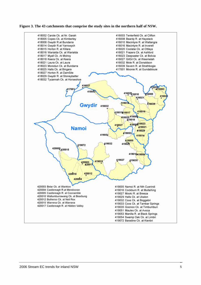
Figure 3. The 43 catchments that comprise the study sites in the northern half of NSW.
2006 Stream EC trends for inland NSW 5
2 Data
2.1 Background
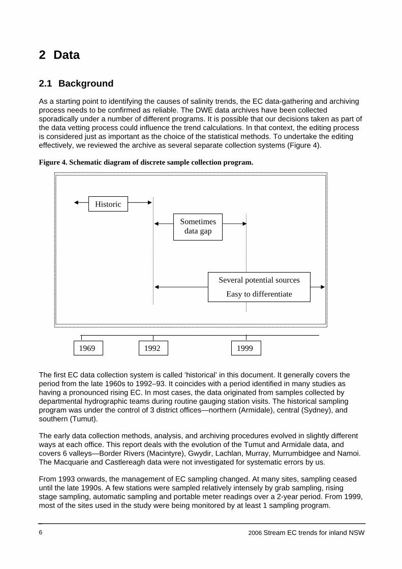
As a starting point to identifying the causes of salinity trends, the EC data-gathering and archiving process needs to be confirmed as reliable. The DWE data archives have been collected sporadically under a number of different programs. It is possible that our decisions taken as part of the data vetting process could influence the trend calculations. In that context, the editing process is considered just as important as the choice of the statistical methods. To undertake the editing effectively, we reviewed the archive as several separate collection systems (Figure 4).
Figure 4. Schematic diagram of discrete sample collection program.
Easy to differentiate
Several potential sources
Sometimes data gap
Historic
19991969 1992
The first EC data collection system is called ‘historical’ in this document. It generally covers the period from the late 1960s to 1992–93. It coincides with a period identified in many studies as having a pronounced rising EC. In most cases, the data originated from samples collected by departmental hydrographic teams during routine gauging station visits. The historical sampling program was under the control of 3 district offices—northern (Armidale), central (Sydney), and southern (Tumut).
The early data collection methods, analysis, and archiving procedures evolved in slightly different ways at each office. This report deals with the evolution of the Tumut and Armidale data, and covers 6 valleys—Border Rivers (Macintyre), Gwydir, Lachlan, Murray, Murrumbidgee and Namoi. The Macquarie and Castlereagh data were not investigated for systematic errors by us.
From 1993 onwards, the management of EC sampling changed. At many sites, sampling ceased until the late 1990s. A few stations were sampled relatively intensely by grab sampling, rising stage sampling, automatic sampling and portable meter readings over a 2-year period. From 1999, most of the sites used in the study were being monitored by at least 1 sampling program.
2006 Stream EC trends for inland NSW 6

The sporadic evolution of the program and diversity of collection approaches have raised questions in this study. For example, is it worthwhile to include marginal data of doubtful quality in order to extend the dataset by several years? We examined each valley as a unique data collection system, and then each station in turn. There was an opportunity to evaluate ‘systems’, but there was insufficient time available to evaluate the work practices of individual staff members.
2.2 Historical EC dataset—(late 1960s to early 1990s)
Routine hydrographic visits to gauging stations usually occurred every 6 weeks or 3 months, with the occasional extra visit to gauge high flows. This means that the historical data set follows a regular pattern. From time to time, gaps appear in the historical record, but in the south of NSW, this is the exception rather than the rule. At the sites used in the Murrumbidgee and Murray valleys, the historical data set generally started in 1969 and finished in the early 1990s. However, at some of the Lachlan Valley sites, it starts a year earlier but cuts out as early as 1987.
A close examination of the historical EC records in TRITON revealed curiosities. In some instances, there was more than one EC value registered on a particular date. The database provided no clarification, flagging the source of the sample analysis as unknown. A preliminary investigation suggested that most of the EC data points during 1969 to 1975 may have been underestimated. This in turn suggests that any rising trend calculations based on the TRITON database might be overestimated. The evidence supporting the existence of the bias is included in Annexure A. It was outside the scope of this study to entirely resolve the database issues, but the implications are discussed in Annexure A.
We planned to examine the Castlereagh and Macquarie sites in a similar way. However, the old hardcopy records could not be easily found. Also, we understood that there was no dual measuring program, because the samples were all transported back to the Sydney laboratory, which was the only measurement location for the 2 valleys.
2.3 Recent EC dataset (1993 to present)
2.3.1 Discrete sampling
After the historical collection program terminated, EC measurements ceased at many gauging sites for about 6 years. There were several exceptions (particularly in the mid Murrumbidgee Valley, where sampling intensified). When regular discrete sampling re-emerged in the late 1990s, the management system had proliferated to a much larger number of locations. This in turn resulted in a variety of sampling methods, frequencies and data quality. For simplicity, the new program is tagged as ‘recent’ in this report. This period of record in the TRITON database has proved the most difficult to review. The quality of the portable meters for measuring EC, the rigour of the meter testing process and the maintenance of standard test solutions vary from office to office. A variety of collection techniques (discussed next) have produced data of varying accuracy.
2.3.2 TRITON (laboratory)
The data in the TRITON database that have been flagged as being ‘laboratory’ analysed are automatically considered suitable for this study. We assume that there are rigorous standards in the collection and analysis of these data.
2.3.3 TRITON (field)
The data flagged as ‘Field’ in TRITON are measured with portable meters in the field, and their accuracy depends on local office protocols. In some instances, the procedure entails adjusting the
2006 Stream EC trends for inland NSW 7

instrument as part of the checking process. It is difficult to track the impact or significance of the changes.
2.3.4 Instrument hydrographer (Tumut)
Data were obtained from the DWE’s HYDSYS database and Tumut office calibration sheets. The instrument hydrographer is an officer based at Tumut and is responsible for the calibration and accurate deployment of in situ EC probes used to provide time-series data. He has extensively evaluated the behaviour of instruments and has a number of accurate instruments at his disposal for comparison. We assume that the measurements he takes during field tests are accurate. Time did not permit an investigation of the equivalent database at Armidale.
2.3.5 Hydrographer portable meters
Data were obtained from the HYDSYS database. The study stations were chosen because they provide flow as well as EC data. Such sites involve routine hydrographic visits. If time-series EC data are collected, then check measurements are undertaken, and these data are available on the HYDSYS database. The instruments used are specifically purchased to measure EC. The disadvantage of this particular system is that not all instruments have calibration documentation.
2.3.6 Rising stage and automatic sample sequences
Over 1992 to 1994, intensive sequence sampling and grab sampling occurred at 4 sites in the Murrumbidgee Valley: 410025 Jugiong at Jugiong, 410044 Muttama at Coolac, 410047 Tarcutta at Old Borambola and 410048 Kyeamba at Ladysmith. All of the samples were analysed in the laboratory. We decided to use the individual grab samples, and to use only 1 sample from each sequence. In the case of automatic sample sequences, this was usually the mid-sequence sample. For the rising stage samples, we adopted the EC value associated with the highest flow.
2.4 Time-series
The time-series data stored in the HYDSYS database are mainly unedited. Their suitability for use in a trend analysis is unknown. We carried out a number of checks to see whether we could quickly edit the data. The data from 10 southern sites are reviewed in Harvey 2006 (in prep.). We concluded that the process of editing would be too time-consuming if the study deadlines were to be achieved. The time-series could be used qualitatively (if needed) to examine the EC characteristics of individual catchments.
2.5 Amalgamation of various EC data systems
The strategy for prioritising the suitability of data since 1992 is as follows:
Time-series EC (Section 2.4) was not used quantitatively because it was not sufficiently edited (Harvey 2006, in prep.).
To match the historical record collection frequency, we set a target of 8 to 12 discrete samples a year from the ‘recent’ record. In most situations, this meant that there was seldom more than 1 data point each month. (For the purpose of comparison with an earlier study, this rule was overlooked at 4 of the sites.)
Use rising stage and automatic sample sequence data, but cull as per Section 2.3.6.
Use all laboratory-analysed data as highest priority.
Use the Tumut instrument hydrographer’s data where available, as priority 2.
Consider hydrographer portable meter reading (if calibration documentation is available).
2006 Stream EC trends for inland NSW 8

Lower priority—data classified ‘field’ in TRITON.
Lower priority—hydrographic portable meters without calibration documentation.
At some sites, the recent record has 1 source only, for example 410061 Adelong at Batlow Road. At other sites, choice is not an issue. For example, at 410091 Billabong at Walbundrie, there is sufficient laboratory data to fulfil frequency requirements, and the other data types were not required for the analysis. At many sites in the north of the State, ‘field’ was conveniently accompanied by laboratory analyses. In such cases, the ‘field’ sample was dropped.
Others undertook the editing and program runs for the Castlereagh, Macquarie and Upper Murrumbidgee and supplied the results to us. The editing procedures are listed in Section 12.
2.6 Groundwater data
We considered including groundwater information in the statistical analysis. In the early stages, it was decided not to, because the process would involve extensive evaluation of numerous bores as a prelude to any editing. At most sites, bore depth measurement frequencies were generally monthly or longer. At a later stage of the study, a method of interpolating these data was developed. Interpolated ground water levels could then be synchronised with the stream EC measurements. The interpolation technique did not reflect short-term fluctuations, but it reflected long-term water table trends.
Another factor worked against the use of bore data. Efficient comparison of the gauging station and groundwater data depends on both being surveyed to a common datum. Without the surveyed information, it is difficult to assess when the deep groundwater tables begins to affect the stream network. Without a common datum, it is difficult to assess the water table gradient between bores.
As a pathfinder investigation, we tried to link the bore data with the stream EC analysis from 8 gauging stations, 4 in the mid Murrumbidgee and 4 in the Namoi. The details are described at the end of the Results section (Section 7.2).
2.7 Catchment characteristics
Jolly et al. (2001) divided the basin into zones. Their concept prompted us to wonder whether the stream EC behaviour could be linked to various catchment parameters. We generated several different characteristics listed below from various geographic information system databases with a view to linking them to catchment EC behaviour.
2.7.1 Elevation at the gauge
The elevation (in m) at the gauging station was measured from a 25-m raster-based digital elevation model (DEM) derived from contour mapping. The numbers produced by this method were used as the default. However, at many sites the gauges had been surveyed to the Australian Height Datum (AHD), and the value of the gauge zero could be used as the stream elevation. If the difference between the DEM and surveyed results was large, then we used the AHD value.
2.7.2 Mean annual rainfall
Mean annual rainfall (mm) was calculated from the Queensland Department of Natural Resources and Mines’ SILO dataset (www.nrm.qld.gov.au/silo), in which daily climatic data from 1956 to 2002 have been interpolated over a 5-km grid. The data in SILO were originally sourced from the Australian Bureau of Meteorology. The mean annual rainfall in each catchment was derived from the rainfall values at a number of grid points within the catchment boundaries.
2006 Stream EC trends for inland NSW 9

2.7.3 Catchment forested (as a percentage)
The Australian Land Cover Change dataset (BRS 2000) was used to indicate the percentage of catchment covered by ‘plantation’ and ‘other woody’ species in 1995.because it contained the most recent data that covered all of NSW.
2.7.4 UPNESS midpoint
‘UPNESS’ is derived from digital elevation data, and is defined as the accumulation of upslope area at any given point’ (Summerell et al. 2005). The ‘midpoint’ is derived objectively from the first inflection point in the normalised cumulative distribution curve of the FLAG UPNESS index (Summerell et al. 2005). In this study, the midpoint value has been used to classify the catchment according to the dominant landforms of steep, even, and flat. The UPNESS value at the midpoint will be lower for steep catchments and greater for open and undulating catchments.
2.7.5 Average slope
The average slope of the catchment was calculated as part of the hypsometric program (Dowling et al. 1998) using contour information from the 25-m DEM. The units are angular degrees.
2.7.6 Hypsometric integral
There were several steps as a prelude to the calculation of the hypsometric integral:
(a) Collation of average slope (Section 2.7.5).
(b) Selection of the elevation contour interval for hypsometric analysis: the smaller the contour interval, the more detailed the analysis. We used 10 m in all catchments, following the methodology of Dowling et al. (1998).
(c) Calculation of minimum and maximum elevation as a prelude to the hypsometric program (Dowling et al. 1998) from the 25-m DEM of the catchment.
Hypsometric (area–altitude) analysis gives a dimensionless parameter that relates the horizontal cross-sectional area of the drainage basin to the relative elevation above the basin mouth. It is said to measure the erosional state or geomorphic age of the catchment (Strahler 1952, Dowling et al. 1998), and has been used in this report as an indicator of catchment verticality. The hypsometric integral allows comparison of catchments regardless of area, and is independent of the absolute height of the catchment above sea level. Mathematically, the integral is the area under the hypsometric curve drawn on axes of relative height and relative catchment area. Its values range from 0 to 1, where lower values have been interpreted by Strahler (1952) to represent older eroded landscapes and higher values to represent young, less eroded landscapes.
2.7.7 Mean EC
This value represents the arithmetic mean of the EC sample data set. Not being flow-weighted, it was vulnerable to bias, but was considered useful as a possible indicator of trend.
2006 Stream EC trends for inland NSW 10

3 Input Dataset
3.1 Final preparation of data
3.1.1 Low flows
The instantaneous flow data used in the study came from the DWE HYDSYS database. Sometimes this information had not been generated in HYDSYS, and it was necessary to go back through the hardcopy record to view the gauging measurement data. If the gauged flow was estimated and was very low, we considered excluding it.
3.1.2 Typographic errors
In preparing data sets, we compared the hardcopy record with the TRITON data. Some of the contradictory data were typographic errors.
3.1.3 Outliers
The dataset from each station was prepared in Microsoft Excel before the S-PLUS script (Appendix 6) was run. By plotting the natural logs (loge) of EC against flow, we could easily identify potential anomalous points. These plots were quickly reviewed, and any anomalies were checked against the data set. On the rare occasions that different sources gave contradictory information, we used the option that plotted better. Otherwise, the outlier was included in the analysis.
3.1.4 Dual data sets
As discussed in Section 2.2, we identified a possible bias in the historical EC record. The details are covered in Annexure A. In the Macquarie and Castlereagh, there was no evidence of a bias. In the Murray, Murrumbidgee and Lachlan, there was insufficient evidence to warrant the use of an altered data set, although it was likely that the EC data for the first few years may have been underestimates. In the Macintyre, Gwydir and Namoi, sufficient evidence existed to warrant an adjustment of +10% to the EC data from the start of the record to 1977 inclusive (Annexure A). These changes have implications for the study conclusions, because they decrease the trend slopes at all sites in these 3 valleys.
Despite having made the definitive decision about data adjustment, we decided to run both data sets through the statistical package (S-PLUS) for all valleys except the Macquarie and Castlereagh. One set was based on the original data, and the other was corrected in the earlier years of record as per Annexure A. This dual run was not time-consuming, but was necessary because the implications of the adjustment could not be assessed until the outputs could be compared.
3.2 Characteristics of input data
We analysed data from 92 gauging stations (Figures 2, 3). With the exception of the 2 sites on the Belubula River, the sites were unregulated. Thirteen of the study sites were subcatchments of larger sites. The sampling frequency was low, and the data points might not be sufficiently representative of the flow range at each station.
Table 1 provides some perspective as to whether the EC samples are taken from a representative flow range at a particular site. It also provides information on the flow behaviour at a particular site.
2006 Stream EC trends for inland NSW 11

The instantaneous flows associated with a specific percentile have been calculated using HYDSYS, and have been generated using hourly instantaneous flow.
Two percentile values are presented. The time-weighted percentile is the percentage of time that a particular flow is exceeded. The flow-weighted percentile is the percentage of total volume that has been recorded whenever a particular instantaneous flow has been exceeded. It is based on the total volume of flow that has passed the site throughout its life. For example, at station 401009, the instantaneous flow of 672 ML/d is exceeded 2% of the time (Column 9). Flows above 2480 ML/d represent 2% of the total volume that passes through the site.
Table 1 provides useful background information on flow behaviour. Columns 3 and 6 list the minimum and maximum instantaneous flows (ML/d). As can be seen from Column 3, flows at many of the sites stop. Column 8 gives a guide to the ephemeral nature of some streams: a zero indicates that there is no flow for at least 50% of the time. Although the time-weighted percentile is a good ephemerality indicator, much of the range may be represented as zero flow. The flow-weighted percentiles are a more sensitive guide because the periods of zero flow are not considered in the calculation.
Table 1 has been used to indicate how representative the EC sampling has been over the site flow range. Column 11 lists the lowest flow associated with an EC sample. Column 12 is the flow-weighted percentile associated with Column 11. It describes where the lowest sample flow fits into the low flow regime. A small number is an indicator of good coverage; in most cases, the Column 12 value encompasses the lower end of the flow regime.
Columns 13 to 15 demonstrate the statistics of the highest flow associated with an EC sample. Column 15 indicates how often the flow is above the sample data set. For example, at site 401009, the highest flow associated with an EC sample is exceeded 2% of the time. On superficial examination at least, the sample data set encompasses the station flow regime most of the time. This suggests that the data set might be a good guide for assessing EC thresholds, where the ‘number of days exceeded’ is the appropriate indicator.
From the perspective of salt-load calculations, the coverage is not as good. Column 14 represents the percentage of the flow distribution not covered by the data set. The higher the percentile, the smaller the flow range encompassed by the EC sampling. At site 401009, 12% of the flows exceed the sample range.
Table 1. Flow duration data (ML/d) showing the extent to which EC sampling represents flows.
Column 1 Column 2 Col. 3 Col. 4 Col. 5 Col. 6 Col. 7 Col. 8 Col. 9 Col. 10 Col. 11 Col. 12 Col. 13 Col. 14 Col.15StationNo. Station Name ML/d %ile ML/d %ile %ile
100
%ile
50 %
ile
2 %
ile
0 %
ile
100
%ile
50 %
ile
2 %
ile
0 %
ile
Low
est
Flow
Flow
W
eigh
ted H
ighe
st
Flow
Flow
W
eigh
ted Ti
me
Wei
ghte
d
401009 Maragle Ck. at Maragle 0.00 255 2480 18810 0.00 45.5 672 18810 0.76 100 978 12 2401013 Jingellic Ck. at Jingellic 0.04 480 7680 16770 0.04 50.0 1150 16770 1.30 100 3550 8 2410091 Billabong Ck. at Walbundrie 0.47 2200 24400 38370 0.47 80.0 3840 38370 2.26 100 3750 37 2410097 Billabong Ck. at Aberfeldy 0.14 387 6610 11630 0.14 6.9 489 11640 0.41 100 1450 23 2410024 Gooradigbee R. at Wee Jasper 7.40 1570 14350 41870 8.17 412.0 4210 41870 20.00 100 4460 16 2410025 Jugiong Ck. at Jugiong 0.00 875 20840 56200 0.00 49.0 1540 56200 0.01 100 12280 5 1410026 Yass R. at Yass 0.00 2640 40980 72430 0.00 23.7 2080 72430 0.01 100 41040 2 1410033 Murrumbidgee R. at Mittagang Xing * * * * * * * * 13.00 * 6890 * *410038 Adjungbilly Ck. at Darbalara 0.18 495 5760 14250 0.18 101.0 1530 14250 0.36 100 4420 4 1410044 Muttama Ck. at Coolac 0.00 895 16700 37160 0.00 14.0 1110 37160 0.10 100 5120 14 1410045 Billabung Ck. at Sunnyside 0.00 955 24220 28960 0.00 0.0 513 28960 0.01 100 6330 20 1410047 Tarcutta Ck. at Old Borambola 0.00 1430 19110 34960 0.00 151.0 3330 34960 2.10 100 25210 1 0410048 Kyeamba Ck. at Ladysmith 0.00 817 10500 19300 0.00 1.9 835 19300 0.04 100 16070 1 0410050 Murrumbidgee R. at Billilingra 0.00 3170 133200 209770 0.00 333.5 6240 209770 1.00 100 18040 19 2410057 Goobarragandra R. at Lacmalac 10.50 1260 8800 26350 10.50 443.0 3340 26350 15.00 99 4230 9 2410061 Adelong Ck. at Batlow Rd. 0.00 185 6280 18280 0.00 59.0 589 18280 4.00 100 649 25 2410062 Numeralla R. at Numeralla School 0.00 3100 63080 75030 0.00 37.9 1920 75030 0.00 100 6900 38 1
Flow Duration Table Flow - Weighted Percentile Time - Weighted Percentile
*: No or insufficient flow data for the percentile assessment.
2006 Stream EC trends for inland NSW 12

Column 1 Column 2 Col. 3 Col. 4 Col. 5 Col. 6 Col. 7 Col. 8 Col. 9 Col. 10 Col. 11 Col. 12 Col. 13 Col. 14 Col.15StationNo. Station Name ML/d %ile ML/d %ile %ile
100
%ile
50 %
ile
2 %
ile
0 %
ile
100
%ile
50 %
ile
2 %
ile
0 %
ile
Low
est
Flow
Flow
W
eigh
ted H
ighe
st
Flow
Flow
W
eigh
ted Ti
me
Wei
ghte
d
410088 Goodradigbee R. at Brindabella 24.40 771 8220 21340 24.60 242.9 2090 21340 28.00 100 7562 2 2410103 Houlaghans Ck. at Downside 0.00 674 9570 10000 0.00 0.0 54 10000 0.00 100 10000 0 0410107 Mountain Ck.at Mountain Ck 0.00 553 8080 20230 0.00 8.0 800 20230 0.20 100 1260 32 2412009 Belubula R. at Canowindra 14.00 2420 28180 46360 14.00 176.0 5020 46360 7.20 100 14100 15 1412028 Abercrombie R. at Abercrombie 0.00 3510 88570 218000 0.00 173.0 6280 218000 0.33 100 19980 14 1412030 Mandagery Ck. at U/S Eugowra 0.00 1140 22100 37400 0.00 31.0 1530 37400 1.10 100 1910 40 2412043 Goobang Ck. at Darbys Dam * * * * * * * * 0.17 * 2830 * *412050 Crookwell R. at Narrawa North 0.00 1310 54000 112000 0.00 54.0 2100 112000 0.36 100 12000 12 1412055 Belubula R. at Bangaroo Bridge * * * * * * * * 0.03 * 3110 * *412065 Lachlan R. at Narrawa 0.00 2730 69200 103400 0.00 93.0 3750 103400 0.20 100 36600 8 1412072 Back Ck at Koorawatha 0.00 682 6960 7140 0.00 3.0 312 7140 0.01 100 3900 11 1412083 Tuena Ck. at Tuena 0.00 694 26320 57400 0.00 11.0 796 57400 0.02 100 3550 20 1412086 Goobang Ck. at Parkes 0.00 201 4840 5240 0.00 1.8 173 5240 0.02 100 1030 19 1412096 Pudmans Ck. at Kennys Rd 0.00 714 12700 27600 0.00 8.3 570 27600 0.02 100 9210 6 1412099 Manna Ck. near Lake Cowal 0.00 11430 23500 23500 0.00 0.0 1770 23500 0.01 100 19800 15 1412103 Bland Ck. at Morangarell 0.00 2970 18000 20000 0.00 0.0 1330 20000 0.70 100 7200 23 1416003 Tenterfield Ck.at Clifton 0.00 977 21900 28500 0.00 12.0 859 28500 0.01 100 2740 31 1416008 Beardy R. at Haystack 0.00 2250 46400 61500 0.00 12.0 1540 61500 0.01 100 5520 33 2416010 Macintyre R. at Wallangra 0.00 5590 122000 150700 0.00 54.0 2750 150700 0.30 100 6210 48 2416016 Macintyre R. at Inverell 0.00 1580 68300 133100 0.00 30.0 1110 133100 0.10 100 1840 48 2416020 Ottleys Ck. at Coolatai 0.02 2650 37700 45100 0.03 4.9 181 45100 0.16 100 1460 60 1416021 Frazer Ck. at Ashford 0.00 3870 71900 78500 0.00 6.2 1710 78500 0.03 100 2040 62 2416023 Deepwater Ck. at Bolivia 0.00 425 12400 13700 0.00 25.5 774 13700 0.01 100 1420 30 1416027 GilGil Ck. at Weemelah 0.00 4840 32050 34000 0.00 50.0 3040 34000 0.10 100 6010 47 1416032 Mole R. at Donaldson 0.00 1620 63800 143000 0.00 71.0 2593 143000 0.06 100 22800 8 1416039 Severn R. at Strathbogie 0.00 3350 46500 71400 0.00 66.0 3590 71400 0.42 100 5360 40 2417001 Moonie R. at Gundablouie 0.00 8190 41000 44700 0.00 0.0 5440 44700 0.06 100 16600 27 1418005 Copes Ck. at Kimberley 0.00 672 21940 35520 0.00 8.5 534 35520 0.05 100 1340 38 1418008 Gwydir R. at Bundarra 0.00 26200 247400 400000 0.00 93.0 10550 400000 0.01 100 26600 40 1418014 Gwydir R. at Yarrowych 0.00 2580 80700 139000 0.00 18.5 1600 139000 0.11 100 9920 30 2418015 Horton R. at Rider 0.00 8710 199000 242000 0.00 69.4 3660 242000 0.30 100 6180 55 1418016 Warialda Ck. at Warialda 0.00 1670 18400 23300 0.00 2.7 382 23300 0.01 100 5020 27 1418017 Myall R. at Molroy with 4/1980 0.08 1720 60000 102500 0.08 10.6 538 102500 0.30 100 834 60 1418018 Keera Ck. at Keera 0.00 569 37460 65360 0.00 10.7 705 65360 0.16 100 910 41 1418021 Laura Ck. at Laura 0.00 650 19900 33300 0.00 7.6 632 33300 0.04 100 935 43 1418023 Moredun Ck. at Bundarra 0.00 1670 28580 30010 0.00 16.6 1360 30010 0.10 100 3630 36 1418025 Halls Ck. at Bingara 0.06 52 19980 37100 0.06 7.7 73 37100 1.80 99 72 44 2418027 Horton R. at Dam Site 0.00 2460 66730 95700 0.00 5.1 840 95700 0.01 100 10180 22 1418029 Gwydir R. at Stoneybatter 0.00 1670 100700 112600 0.00 69.5 2455 112600 0.37 100 4700 31 1418032 Tycannah Ck. at Horseshoe Lagoon 0.00 4830 55560 57100 0.00 3.2 485 57100 0.10 100 10000 36 1418052 Carole Ck. near Garah 0.00 580 8260 9940 0.00 62.0 1370 9940 0.10 100 2490 17 1419005 Namoi R. at Nth Cuerindi 0.00 2430 71800 130000 0.00 161.0 71800 130000 1.10 100 11300 22 1419016 Cockburn R. at Mulla Crossing 0.00 1960 32900 64500 0.00 24.0 1760 64500 0.02 100 6249 28 1419027 Mooki R. at Breeza 0.00 16600 144000 158000 0.00 9.5 2710 158000 0.03 100 90600 14 1419029 Halls Ck. At Ukalon 0.00 324 15200 21140 0.00 6.9 391 21140 0.57 100 1070 25 1419032 Coxs R. at Boggabri 0.00 17000 111300 115000 0.00 0.0 1320 115000 0.07 100 4890 74 1419033 Coxs R. at Tambar Springs 0.00 6670 45400 48000 0.00 6.1 307 0 0.30 100 624 74 1419035 Goonoo Goonoo Ck. at Timbumburi 0.00 1390 33940 43700 0.00 7.9 387 43700 0.12 100 3310 40 1419051 Maules Ck. at Avoca * * * * * * * * * * * * *419053 Manilla R. at Black Springs 0.00 1440 79500 116000 0.00 18.0 580 116000 0.70 100 7280 31 1419054 Swamp Ck. At Limbri 0.00 743 28320 56900 0.00 7.1 699 56900 0.07 100 1230 39 1419072 Baradine Ck. at Kienbri 0.00 1270 18500 24340 0.00 0.0 307 24340 0.16 100 2960 35 1420003 Belar Ck. at Warkton 0.01 255 5720 12920 0.01 4.3 205 12920 0.38 100 4200 5 1420004 Castlereagh R. at Mendooran 0.00 4980 65290 82730 0.00 26.9 1527 82730 0.03 100 31640 17 1420005 Castlereagh R. at Coonamble 0.00 5640 57400 61330 0.00 7.8 3380 61330 0.11 100 61160 0 0420010 Wallumburrawang Ck. at Bearbung 0.00 652 7400 20610 0.00 0.0 238 20610 0.01 100 1750 28 1420012 Butheroo Ck. at Neilrex 0.00 1580 22000 25840 0.00 0.2 130 25840 0.00 100 622 67 1420015 Warrena Ck. At Warrana 0.00 1860 6870 7410 0.00 0.0 356 7410 0.00 100 3690 30 1420017 Castlereagh R. at Hidden Valley 0.00 2415 75380 98450 0.00 12.0 833 98450 0.02 100 3865 43 1421018 Bell R. at Newrea 0.00 1754 79150 104300 0.00 61.0 2090 104300 0.20 100 17780 15 1421023 Bogan R. at Gongolgon 0.00 8080 144200 220000 0.00 50.5 8660 220000 0.38 100 46930 63 1421025 Macquarie R. at Bruinbun 0.00 3970 154400 232200 0.00 249.2 7390 23200 1.58 100 14820 22 2421026 Turon R. at Sofala 0.00 2040 104900 154200 0.00 36.3 1630 154200 0.03 100 63020 6 1421035 Fish R. at Tarana 0.00 724 33440 55860 0.00 106.5 1670 55860 0.41 100 2160 21 2421039 Bogan R. at Neurie 0.00 9080 49600 58200 0.00 0.0 3180 58200 0.02 100 2750 74 2421042 Talbragar R. at Elong 0.00 2100 42630 65130 0.00 16.0 1170 65130 0.12 100 14640 16 1421048 Little R. at Obley 0.00 1460 42780 48080 0.00 6.1 840 48080 0.10 100 4080 99 1421055 Coolbaggie Ck. at Rawsonville 0.00 3830 19510 20670 0.00 0.0 431 20670 0.02 100 15960 4 1421056 Coolaburragundy R.at Coolah 0.00 181 12400 32100 0.00 8.1 166 32100 0.17 100 617 39 1421059 Buckinbah Ck. at Yeoval 0.22 14.9 640 1260 0.22 7.4 43 1260 0.08 100 478 3 1421072 Winburndale Rivulet at Howards Bge 0.00 1275 66210 70350 0.00 43.0 1600 70350 0.40 100 66270 2 0421073 Meroo Ck. At Yarrabin2 * * * * * * * * 0.17 * 6680 * *421076 Bogan R. at Peak Hill 0.00 2770 28740 29470 0.00 0.0 619 29470 0.93 100 6100 31 1421084 Burrill Ck. At Mickibri 0.00 327 6630 6380 0.00 0.0 109 8380 0.06 100 310 51 2421101 Campbells R. atU/S BenChifley Dam 0.00 861 37100 67200 0.00 45.6 1480 67200 0.04 100 4170 21 1
Flow - Weighted Percentile Time - Weighted Percentile
Flow Duration Table
In general, the flow-weighted percentile column (14) suggests that the coverage of the sampling might extend into the high flow range at some sites. This is particularly the case for the data sets from southern NSW. On first view, this might be seen as cause for optimism, because
2006 Stream EC trends for inland NSW 13

comprehensive representation across the flow range might point to robustness in the development of any mathematical equations. Unfortunately, the following information offsets any illusion that the high flow EC is well represented.
In the early part of this investigation, we hoped to run the trend analysis models for event and base flow separately. As a consequence, the sample sets for 12 of the southern sites were separated into event and base flow, using the separation method described in Harvey and Jones (2001). The percentages of runoff event samples were low, varying from 13% to 34% of the data set at each site. At most sites the event sampling ratio was as low as 1 in 5. It is not clear whether these small percentages are sufficient to adequately extend the EC–flow relationship into the high flow ranges. There must be some optimism that the subsequent trend analysis extends beyond base flow conditions. Base flow data sets have been modelled, and the results are provided in Section 7.1.
To understand how well the high flows were represented in the EC sampling across NSW, we developed histograms showing where the highest sample sat in each flow range. The data are drawn from Column 14. Four bar charts are presented in Figure 5. A small percentile value (on the X axis) is an indication of a high flow. The first quadrant covers the whole State, where 87 of the 92 sites have flow duration information. The State has been divided arbitrarily into north, centre and south. The partitioning is based on the old DWR management structure and on the assumption that different strategies may have been used for data collection in each district.
Two aspects of Figure 5 are of interest. If the highest sample flow is in the 0 to 20 percentile range, then there might be a case for claiming an understanding of EC behaviour for high flows at a particular site. A high proportion of the southern sites fall in the 0 to 20 percentile range, whereas few of the northern sites have a high flow coverage.
We also wanted to identify sites with a poor representation of high flow range. The 50 to 100 percentile range indicates no incorporation of higher flows’ EC in the trend calculations. There can be little confidence in any results from 11 such sites (none in southern NSW).
2006 Stream EC trends for inland NSW 14
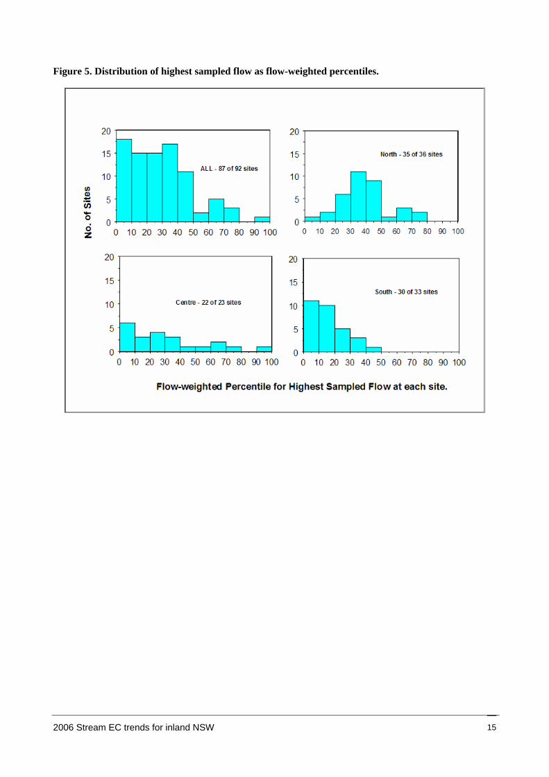
Figure 5. Distribution of highest sampled flow as flow-weighted percentiles.
2006 Stream EC trends for inland NSW 15

4 Statistical Methodology
4.1 Aim
The aim of this data analysis is to obtain estimates of stream salinity trends that are independent of season of observation and fluctuations in river flow rates and, hence, indicate the impacts of catchment salinisation on stream EC.
4.2 Background
Much of the technical details of the statistical trend analysis performed in this report originate from work developed by Richard Morton, a biometrician in the Mathematical and Information Sciences unit of CSIRO in Canberra.
Early work by Morton (Cunningham and Morton 1983; Morton and Cunningham 1985) concentrated on using time-series analysis to model the salinity trend at stations on the River Murray. Cunningham and Morton (1983) worked on 43 years (517 monthly readings) of chloride data from Morgan, SA. They proposed a model that had deterministic components that included a time trend, together with seasonality and flow measurements. The random component of their model was formed as a first-order autoregressive process. Morton and Cunningham (1985) extended this work when analysing 16 years of monthly EC data from 8 stations on the Murray. Instead of analysing each station in isolation, they developed a predictive model for a downstream station by including data from an upstream station, which effectively accounted for spatial correlation between stations.
Later work (Morton 1997a, b) introduced semi-parametric models for the estimation of trends in stream salinity. The method combined elements of Generalised Additive Models (GAMs) and time-series analysis to account for serial correlation over time. Application of this method can be found in Jolly et al. (1997, 2001), Walker et al. (1998), Nathan et al. (1999) and Smitt et al. (2002).
More recently, Morton (2002) provided the NSW Department of Land and Water Conservation (now DWE) with a review of potential statistical methods for the detection and estimation of trends in water quality. They concluded that GAMs are preferable when the trend is non-linear and autocorrelation is present. Morton and Henderson (2002) applied these methods to data originating from DWE’s ‘Key Sites’ project (Preece 1998).
4.3 Formulation of the model
The statistical methods used in the trend analysis exploit semi-parametric regression models. In semi-parametric models, arbitrary smooth curves are fitted in place of parametrically defined curves such as straight lines or polynomials (Figure 6). Models using these curves are commonly referred to as GAMs. The smooth curves are ‘non-parametric’ in the true sense of the term, in that the smooth function does not have a parametric form. ‘Semi’ implies that some regression terms may be represented parametrically. Unlike polynomials, spline curves are usually suitable for short-term prediction because they are often straight near the extremes.
Harvey and Jones (2001) reported an example of a flat spline at the EC versus flow extremity. They observed that the low flow regime was not the major driver of EC. Rather, time elapsed after the peak (in days) seemed to have greater affinity with EC.
2006 Stream EC trends for inland NSW 16

Figure 6. Comparison of polynomial and smoothing spline curves on irregularly shaped data.
Graphic is copied from Venables and Ripley (1994).
Smooth curves can be estimated by various methods, including splines, kernels and locally weighted regression (LOWESS). Hastie and Tibshirani (1990) give an excellent account of such methods.
Weaknesses with previous approaches to trend analysis were that the methods generally assumed the starting date for a temporal trend to be the beginning of the time-series and, more often than not, that trends were linear over time. They also had no effective way of modelling non-linear fluctuations with time other than by fitting higher-order polynomials. In addition, the relationship between salinity and flow is often marked by an absence of any correlation in low flows. A GAM, however, can not only fit the time trend as an arbitrary smooth spline, but it can also fit the flow term as an arbitrary smooth curve, thereby allowing a flexible method of correcting for flow effects (often called a nuisance variable in the statistical literature). Other additive terms can be incorporated into the regression model, and season can be represented as a sinusoidal curve. Thus, there is considerable flexibility in using this modelling approach.
The regression methodology fitted the GAMs using an ordinary least squares algorithm, assuming errors to be independent and normally distributed.
The analyses were carried out with S-PLUS (Insightful Corp. 2003) v. 6.2 statistical software, and were based on the natural logarithms of flow and EC. Log-transformation was used for 3 main reasons. Firstly, we found that flow effects acted proportionately on EC and hence additively on the loge scale. Secondly, the log-transform stabilised the variance. Thirdly, the transformation reduced the right skewness and so was likely to make the error distribution more symmetrical. Moreover, we found that the relation of logeEC to logeflow was approximately linear in most of the data sets, which simplified the adjustment of EC for flow. Also, as described in Section 4.5, the
2006 Stream EC trends for inland NSW 17

linear trend is easily estimated from the loge transformation as a percentage change in trend (compounded).
A copy of the S-PLUS script file is given in Appendix 6. Users are advised to apply the script file at their own risk, as the process requires considerable statistical experience and understanding. The analysis should never be considered to be an ‘automatic’ or a ‘robotic’ process. An annotated output from running this script file on one data set is given in Appendix 7.
The mathematical form of the regression model used was:
logeEC = α + S1(logeflow; dff) +
β sin(2π Yday / 365) + γ cos(2π Yday / 365) + S2(time; dft) + ε, (1)
where:
logeEC is the natural logarithm of EC
logeflow is the natural logarithm of flow
Yday is the numeric day of the year (1 … 365), e.g. 2 October 1988 = 276
time is a decimal variate of date of observation, e.g. 2 October 1988 = 1988 + (276 / 365) = 1988.756
S1(logeflow; dff) is a smoothing spline of logeEC vs logeflow with dff degrees of freedom
S2(time; dft) is a smoothing spline of logeEC vs time with dft degrees of freedom
α, β, γ are linear regression coefficients to be estimated
ε is the normally distributed residual error, which may or may not possess serial correlation.
The terms dff and dft are smoothing parameters that determine the shape of the splines fitted to the data. We have adopted Morton’s (1997b) recommendation of smoothing parameters set at 2 for logeflow and 4 for time trend. In heuristic terms, the amount of non-linearity accommodated in the model is roughly similar to that found in a polynomial of degree 2 or 4 (quadratic or quartic), although the shape of the fitted curve is not constrained to that of a polynomial. As assumed by Morton and Henderson (2002), the form of the logeflow effect is considered to be very smooth, hence dff = 2. The trend in time is expected to be less regular, with dft = 4 allowing for a non-linear curve of reasonable complexity. We agree with Morton and Henderson (2002) that ‘where data exist for less than 8 years, the spline with dft = 4 may be undersmoothing the time trend’. Since the data used in the study are at times half as regular as Morton and Henderson’s monthly data, sites with less than 16 years of data may require using dft = 2 rather than 4. Thus, time trend and logeflow followed non-parametric curves, whereas season had a parametric form.
4.4 Graphical insight into model structure
Equation 1 embodies a complex but necessarily flexible formula of explanatory variables that may affect stream EC. Essentially, the formula needs to be adaptable in order to maximise its chances of suitably fitting the 100+ individual sites that make up the stream EC study.
This section has been written to help the reader develop an understanding of the influence of each component of the GAM on stream EC by graphically examining different elements of the model.
To obtain estimates of stream salinity trends that are independent of season of observation and of fluctuations in river flow rates, various relationships need to be quantified for each site. Initially, we focus on the relationship between logeEC and logeflow. Figure 7 shows the extent to which the EC–flow relationship can differ between sites.
2006 Stream EC trends for inland NSW 18
2006 Stream EC trends for inland NSW 19
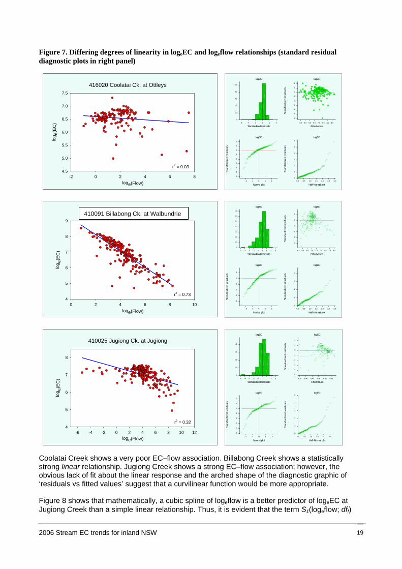
Figure 7. Differing degrees of linearity in logeEC and logeflow relationships (standard residual diagnostic plots in right panel)
Coolatai Creek shows a very poor EC–flow association. Billabong Creek shows a statistically strong linear relationship. Jugiong Creek shows a strong EC–flow association; however, the obvious lack of fit about the linear response and the arched shape of the diagnostic graphic of ‘residuals vs fitted values’ suggest that a curvilinear function would be more appropriate.
Figure 8 shows that mathematically, a cubic spline of logeflow is a better predictor of logeEC at Jugiong Creek than a simple linear relationship. Thus, it is evident that the term S1(logeflow; dff)
410025 Jugiong Ck. at Jugiong
loge(Flow)-6 -4 -2 0 2 4 6 8 10 12
log e
(EC
)
4
5
6
7
8
r2 = 0.32
logEC
logEC
logEC
logEC
1 3
3
1
2.51.5
0
0.5
10
Half-Normal plot
20
-5
30
-3
40
-2
50
60
70
0
-2
-4
20-2
Fitted values-1 6.4 6.6 6.8
2
7.0 7.2 7.4
3.0
7.6
1.0
7.8
Standardized residuals8.0
-1
-3
1
Normal plot
2
0
0.0
-4
1
-3
-2
0
-1
0
-4
1
4
2.0-1
Sta
ndar
dize
d re
sidu
als
Sta
ndar
dize
d re
sidua
ls
Sta
ndar
dize
d re
sidu
als
logEC
logEC
logEC
logEC
0-2
Normal plot
-1
5
0
3
1
1
2 3
2.51.50.5
Half-Normal plot
-5 -3 -2
0
10
20
30
40
1
-1
-3
-5
2
Fitted values6.35 6.40
4
6.45
0
6.50 6.55 6.60
1.0
Standardized residuals
2
-2
-4
1
-5
-4
-3
2.0
-2
-4
-1
0
0
1
2
2
0.0-1
Sta
ndar
dize
d re
sidua
lsS
tand
ardi
zed
resid
uals
Sta
ndar
dize
d re
sidua
ls
logEClogEC
logEC logEC
0-1-2
Normal plot
0
6
2
4
4
2
0
3.02.0
0
1.0
20
0.0
40
Standardized residuals
60
-4
80
100
2
0
-2
-4
Fitted values
-6
5.0 5.5 6.0 6.5
2
7.0 7.5 8.0
5
8.5
1
2.50.5
-6
-1
-5
-6
-5
-4
-3
3
-2
-1
1.5
0
-2
1
2
-3
1
Half-Normal plot
1
Sta
ndar
dize
d re
sidua
lsS
tand
ardi
zed
resi
dual
s
Sta
ndar
dize
d re
sidu
als
416020 Coolatai Ck. at Ottleys
loge(Flow)-2 0 2 4 6 8
log e
(EC
)
4.5
5.0
5.5
6.0
6.5
7.0
7.5
r2 = 0.03
410091 Billabong Ck. at Wallabundrie
loge(Flow)0 2 4 6 8 10
log e
(EC
)
4
5
6
7
8
9
r2 = 0.73
410091 Billabong Ck. at Walbundrie

2006 Stream EC trends for inland NSW 20
within Equation 1 is capable of suitably fitting such non-linear relationships. In situations where this curvature is absent, the spline function would default back to a simpler linear response function.
Figure 8. Fitting a spline function of logeflow to logeEC (standard residual diagnostic plots in right panel)
The formula obtained for the EC–flow relationship is now used to derive an estimate of EC that has been adjusted for differences caused by stream flow. This adjustment process is depicted in Figure 9. Using the linear relationship for Billabong Creek as an example, observed logeEC values are numerically ‘walked’ up and down imaginary lines (which run parallel to the linear regression line) to the point of average logeflow. The average logeflow is shown by a vertical line at an equivalent logeflow of 4.32. The left panel of Figure 9 shows that a high reading for logeEC may be primarily due to the fact that this record was taken at a time of low logeflow. Similarly, a low logeEC reading may be due to the existence of a high logeflow. The right panel of Figure 9 shows the full corrected EC dataset for Billabong Creek, having been adjusted to the mean logeflow.
Figure 9. Calculation of ‘EC adjusted for flow’.
Grey symbols: unadjusted EC; red symbols: flow-adjusted EC values.
Another variable which may add ‘unwanted noise’ to the efficient estimation of long-term stream salinity trends is periodicity of EC levels. For the Gwydir River at Bundarra, Figure 10 shows the effect of fitting the seasonality terms β sin(2π Yday / 365) + γ cos(2π Yday / 365) (Equation 1) to the flow-adjusted logeEC data. Although the compressed time scale axis makes it difficult to immediately appreciate the positive benefits of including these terms (Figure 10, top panel), magnification of part of the time axis (Figure 10, bottom panel) reveals a sinusoidal pattern within the flow-adjusted EC data.
410025 Jugiong Ck. at Jugiong
loge(Flow)-6 -4 -2 0 2 4 6 8 10 12
log e
(EC
)
4
5
6
7
8
r2 = 0.50
logEClogEC
logEC logEC
1 2 3
4
2
0
3.02.01.0
0
0.0
10
Standardized residuals
20
-4
30
40
50
60
70
2
0
-2
-4
20-2
Fitted values-2 6.00 6.2 6.4
3
6.6 6.8 7.0 7.2
1.5
7.4
Half-Normal plot
-3
-1
-3
1
Normal plot
1
-4
0.5
-3
-2
1
-1
0
-1
1
2
-5
2.5-1
Sta
ndar
dize
d re
sidua
lsS
tand
ardi
zed
resid
uals
Sta
ndar
dize
d re
sidua
ls
logEC vs logFlow
410091 Billabong Ck. at Wallabundrie
loge(Flow)0 2 4 6 8 10
log e
(EC
)
4
5
6
7
8
9
logEC vs logFlow
410091 Billabong Ck. at Wallabundrie
loge(Flow)0 2 4 6 8 10
log e
(EC
)
4
5
6
7
8
9

Figure 10. Modelling seasonality within EC trends.
r2 = 0.22
418008 Gwydir R. at Bundarra
Year
1970 1980 1990 2000
Flow
adj
uste
d lo
g e(E
C)
4.0
4.5
5.0
5.5
6.0
6.5
7.0
7.5
Year
1998 1999 2000 2001 2002 2003 2004
In a manner similar to that described for adjusting for differences in flow, EC data are further adjusted for common periodic patterns within each year. Figure 11 illustrates how data that follow the ‘high’ side of the fitted sinusoidal curve are adjusted downwards, and data that follow the ‘low’ side of the curve are adjusted upwards.
Figure 11. Calculation of EC adjusted for flow and seasonality. Grey symbols: flow-adjusted EC; red symbols: flow- and seasonally adjusted EC values.
418008 Gwydir R. at Bundarra
Year
1998 1999 2000 2001 2002 2003 2004
Adju
sted
log e
(EC
)
4.0
4.5
5.0
5.5
6.0
6.5
7.0
7.5
2006 Stream EC trends for inland NSW 21

Once these ‘corrections’ to the logeEC data have been completed, a more accurate view of the trend of logeEC over time can be made. The 3 panels in Figure 12 indicate the range of trends of logeEC over time. These plots indicate that the flexibility of the spline term for time (Equation 1) was essential to adequately model the variety of time responses evident in this project.
The plot for Maragle suggests that up until the mid 1990s, logeEC was tending to increase. However, a relative decline is evident from 2000. The panel for Jugiong Creek implies that logeEC was also increasing to the mid 1990s, and has flattened somewhat throughout the early 2000s. The third panel shows that the Belubula River trend has remained almost negligible over the period of observation.
These changing trends have significant impacts on the ability and confidence with which future predictions of logeEC can be made, as is discussed in Section 4.5.
Figure 12. Differing degrees of curvature of adjusted EC over time.
logEClogEC
logEC logEC
-2-3
Normal plot
2 4
4
2
0
0
3.0
10
2.0
20
1.0
30
0.0
40
Standardized residuals
50
-2
60
70
80
3
1
-1
-3
-5
Fitted values4.45
3
4.50
1
4.55
-1
4.60 4.65
5
4.70
1
4.75 4.80
2.50.5
-4
0
-4
-5
2
-4
-3
3
-2
-1
1.5
0
0
1
2
-2
3
0
Half-Normal plot
2
Sta
ndar
dize
d re
sidua
ls
Sta
ndar
dize
d re
sidua
ls
Sta
ndar
dize
d re
sidua
ls
401009 Maragle at Maragle
Year
1970 1980 1990 2000
Flow
& s
easo
nally
adju
sted
log e
(EC
)
3.0
3.5
4.0
4.5
5.0
5.5
6.0
410025 Jugiong Ck. at Jugiong
Year
1970 1980 1990 2000
Flow
& s
easo
nally
ad
just
ed lo
g e(E
C)
5.5
6.0
6.5
7.0
7.5
8.0
logEClogEC
logEC logEC
0 1 2 3
4
2
0
3.02.01.00.0
0
Standardized residuals
10
-4
20
30
40
50
60
70
3
1
-1
-3
-5
20
Fitted values
-2
6.6-2 6.7 6.8 6.9
1
7.0 7.1 7.2
2.50.5
-5
0
-4
-5
-1
-4
-1
-3
3
-2
-1
1.5
0
-3
1
2
-2
3
Normal plot Half-Normal plot
2
1
Sta
ndar
dize
d re
sidua
ls
Sta
ndar
dize
d re
sidua
ls
Sta
ndar
dize
d re
sidua
ls
2006 Stream EC trends for inland NSW 22

412009 Belubula R. at Canowindra
Year
1970 1980 1990 2000
Flow
& s
easo
nally
ad
just
ed lo
g e(E
C)
5.2
5.6
6.0
6.4
6.8
7.2
7.6
logEClogEC
logEC logEC
0-1-2
Normal plot
2
4
4
2
6
0
3.02.01.0
0
0.0
10
Standardized residuals
20
-2
30
40
50
60
70
5
3
1
-1
-3
2
Fitted values6.30 6.35
3
6.40 6.45 6.50
1.5
Half-Normal plot
0
4
2
0
-3
-2
1
-1
5
0
1
2.5
2
-4
3
4
-2
5
1
0.5
Sta
ndar
dize
d re
sidua
ls
Sta
ndar
dize
d re
sidua
ls
Sta
ndar
dize
d re
sidua
ls
4.5 Interpretation of analysis It is important to note that each term of the form S(x; m) is the sum of the linear component (of the form a + b·x) and the non-linear component (which has a mean of zero and no linear trend) of the trend. By separating the linear and non-linear components of the spline function, we can expand the spline terms in Equation 1 to:
S(x; m) is the sum of the linear component (of the form a + b·x) and the non-linear component (which has a mean of zero and no linear trend) of the trend. By separating the linear and non-linear components of the spline function, we can expand the spline terms in Equation 1 to:
logeEC = α + S1(logeflow; dff) + β sin(2π Yday / 365) + γ cos(2π Yday / 365) + S2(time; dft) + ε, logeEC = α + S1(logeflow; dff) + β sin(2π Yday / 365) + γ cos(2π Yday / 365) + S2(time; dft) + ε,
χ logeflow + ClogeFlow η time + Ctime χ logeflow + ClogeFlow η time + Ctime
where χ and η are the linear coefficients of logeflow and time respectively, and ClogeFlow and Ctime are the non-linear components of S1(logeflow; dff) and S2(time; dft). where χ and η are the linear coefficients of logeflow and time respectively, and ClogeFlow and Ctime are the non-linear components of S1(logeflow; dff) and S2(time; dft).
When we are most interested in the overall linear trend in EC per year over the period of observation, the linear coefficient of time, η, is relevant; η was used to calculate the percentage change in EC per annum (compounded) using the formula:
When we are most interested in the overall linear trend in EC per year over the period of observation, the linear coefficient of time, η, is relevant; η was used to calculate the percentage change in EC per annum (compounded) using the formula:
100 × (eη – 1). (2) 100 × (eη – 1). (2)
Derivation of this formula is explained in Appendix 8. Derivation of this formula is explained in Appendix 8.
As was shown by Cunningham and Morton (1983), estimates of the standard error (SE) of η can be used with compound interest formulae to derive confidence limits (CLs) for the net percentage increase (or decrease) over the full period of observation:
As was shown by Cunningham and Morton (1983), estimates of the standard error (SE) of η can be used with compound interest formulae to derive confidence limits (CLs) for the net percentage increase (or decrease) over the full period of observation:
linear coefficient = lc = η (from printout of analysis of logeEC) linear coefficient = lc = η (from printout of analysis of logeEC)
upper limit = ul = η + 1.969 × SE upper limit = ul = η + 1.969 × SE
lower limit = ll = η – 1.969 × SE lower limit = ll = η – 1.969 × SE
proportional change in EC p.a. = pc = (eη – 1) proportional change in EC p.a. = pc = (eη – 1)
upper limit = pu = (eul – 1) upper limit = pu = (eul – 1)
lower limit = pl = (ell – 1) lower limit = pl = (ell – 1)
% change over period = %c = 100 × {pc × (1 + pc)years – pc} / pc % change over period = %c = 100 × {pc × (1 + pc)years – pc} / pc
upper limit = %u = 100 × {pu × (1 + pu)years – pu} / pu upper limit = %u = 100 × {pu × (1 + pu)years – pu} / pu
lower limit = %l = 100 × {pl × (1 + pl)years – pl} / pl lower limit = %l = 100 × {pl × (1 + pl)years – pl} / pl
2006 Stream EC trends for inland NSW 23

As an example of using these formulae, a typical site may have, say, 43 years of data, a linear trend coefficient on the loge scale of 0.0018, with an SE of 0.00058. This equates to a percentage change per annum (compound) of 1.43%, with 95% CLs of (0.0409%, 2.84%). For the period spanned by the data, namely 43 years, the percentage is compounded, giving the estimated increase as 84.2% with CLs (1.8%, 233.4%).
This example serves as a warning of the potential inaccuracies that may occur from data such as these in the estimation of trend parameters and in forming future predictions.
Another warning needs to be given to those who may mistakenly consider that the linear trend is the only statistic of interest. Morton (2002) reminds us that the trend may be markedly non-linear, in which case the linear trend component does not give an adequate summary of the trend. When interpreting this type of trend analysis, note must be taken of the significance of the non-linear component Ctime. It should be obvious to all readers that extrapolation or prediction of such trends into the future is fraught with danger, and especially so in the presence of a significant non-linear time component.
The linear trend is not to be taken as suitable for extrapolation, as it becomes exponential on the original scale, and there is no guarantee that it remains linear on the logarithmic scale. Plotting the form of the non-linear trend over time after removing the influences of flow and season by including a LOWESS smoother is a useful exploratory tool.
4.6 Correlated residual terms It is commonly found that data recorded over time possess serial correlation. The strength of serial correlation will depend on the degree of contribution of all processes generating these data, relative to random noise; the correlation will also be influenced by the physical time lag between successive observations. Thus, it may be expected that the degree of serial correlation exhibited by data examined by Morton and Henderson (2002) could be somewhat higher than that found in the present study. This expectation occurs because Morton and Henderson used monthly data observations collected largely from regulated rivers with ‘more uniform’ flow patterns. In small streams with characteristically peaky flows, autocorrelation is often not an issue. This report uses data collected approximately every 2 months, and originates from third-order unregulated rivers and streams.
Notwithstanding this, a positive serial correlation within the residual terms will influence the interpretation of output from this analysis. Morton and Henderson (2002) clearly state that the regression estimates given by this method are generally accurate in themselves, but the formal SEs and CLs formed around the estimates are misleadingly small. That is, a positive autocorrelation has the effect of reducing the formal statistical significance of estimated time trends. This results in estimates of trend that appear to have greater precision than they deserve.
Morton and Henderson (2002) generalised this model even further for a ‘complete’ dataset (that is, when <20% of the monthly data are missing). They accommodate serial correlation in the residuals by fitting the regression as a time-series model, assuming that the residuals follow a first-order autoregressive process with autocorrelation coefficient ρ. They suggest a threshold of ρ > 0.2 as being sufficiently high to invalidate SEs and confidence intervals (CIs).
Morton has suggested a workaround for datasets that have >20% of monthly values missing, as is common in the present analysis. Under Morton’s biometrical guidance, Jolly et al. (1997) provide a formula to calculate an adjustment factor used to increase the otherwise misleadingly small SEs of estimates. In this case, the SEs from the statistical output are adjusted for the magnitude of the autocorrelation and amount of missing data by multiplying by the following factor:
2006 Stream EC trends for inland NSW 24

2006 Stream EC trends for inland NSW 25
⎥⎦⎣ − ACF1 (3)
⎤⎢⎡ +
ACFP**21
where
P is the proportion of available data
ACF is the first-order autocorrelation coefficient.
Morton and Henderson (2002) remind us of Morton’s (1997a) approximation to this multiplier, formed when there are no missing data (P is assumed to be unity). This approximation is:
(4)
Morton and Henderson have found reasonable agreement between the SE of a linear trend component derived either by the adjustment of ordinary least squares estimates of error or by applying a ‘proper’ time-series method.
We acknowledge that the estimate of the (lag 1) autocorrelation coefficient used here is approximate, as the data have not been recorded at regular time intervals. Nevertheless, we have adopted a conservative approach to the estimation of the precision of the linear trend, and our analysis includes the derivation (and tabulation) of a first-order autocorrelation coefficient, and uses the approximate multiplying factor from Equation 4 when deriving SEs and CLs of trend estimates. The whole process of estimation and prediction is therefore an approximation.
4.7 Model hierarchy
Equation 1 represents a reasonably sophisticated model that has been fitted in a single operation by previous workers. For this analysis, we have fitted it in incremental steps, initially to better monitor and understand the progress of the individual components of the model (Figure 13). The incremental fitting procedure also allowed investigation of the contribution of each additional term in a hierarchical sense, and allowed the exploration of other potential explanatory variates, such as groundwater, to be included in future trend analyses.
Models 1 to 3 (Figure 13) examined logeEC versus logeflow, with a seasonality component added. Models 4 and 5 examined flow-adjusted EC as a function of time. Models 6 and 7 fitted EC as a function of all explanatory variables, namely instantaneous flow, seasonality and time.
Model 7 fits a GAM, with spline terms for flow and time. We considered Models 3, 5 and 7 to be of most interest, since each represents a more sophisticated equation for, respectively, logeEC vs logeflow, flow-adjusted logeEC vs time, and logeEC as a function of logeflow, seasonality and time.
The mean of the observed logeflow was calculated for each sample data set. Model 7 was then solved to predict logeEC over the time period of observation, using average logeflow and seasonality effects. The average logeflow at each site is tabulated in Appendix 1.
Results from these analyses were summarised using statistics and plots. The relevant statistics are presented in a number of tables throughout this report. S-PLUS was used to generate graphical representations of many steps of the analyses. The final plot generated a logeEC spline curve fitted at the mean logeflow and seasonality over the period of observation. These plots are presented in Appendix 2.
⎥⎦⎣ − ACF⎤
⎢⎡ + ACF
11

Figure 13 also indicates that groundwater was used as an additional explanatory variable in a pilot study of 8 gauging stations. We postulated that a groundwater smoothing spline accounted for additional variation in logeEC not explained by other variables in the model (Models 3a and 7a).
Figure 13. Flow chart of hierarchical model sequence. Model 7 was of primary interest. The benefits of including groundwater data were explored in Models 3a and 7a.
(1) loge(EC) ~ loge(Flow)
(2) loge(EC) ~ loge(Flow) + sin(time) + cos(time)
(3) loge(EC) ~ s[loge(Flow),2] + sin(time) + cos(time)
(7) loge(EC) ~ s[loge(Flow),2] + sin(time) + cos(time) + s[yrfrac,4]
(4) Flow adj[loge(EC)] ~ yrfrac(5) Flow adj[loge(EC)] ~ s[yrfrac,4]
(3a) loge(EC) ~ s[loge(Flow),2] + sin(time) + cos(time) + s[groundwater,2]
(7a) loge(EC) ~ s[loge(Flow),2] + sin(time) + cos(time) + s[groundwater,2] + s[yrfrac,4]
(6) loge(EC) ~ loge(Flow) + sin(time) + cos(time) + yrfrac
4.8 Trend indicators
Jolly et al. (2001) represented EC trend as linear on a loge scale. The various curves in Jolly et al. (1997) implied cyclic behaviour at some sites. Harvey and Jones (2001) noted a decrease in the rising EC trend at some of their sites. As one of our study goals was to quantify trends, it was essential to have a classification or quantification that considered cyclicity (non-linearity). As the project evolved, the non-linear component of the GAM graphs became increasingly important in the interpretation of the processes.
4.8.1 Statistical linearity
The first method used to indicate trend was based on the statistical approach of Jolly et al. (1997). Statistical routines were used to:
quantify the linear trend on loge scale
determine whether this linear trend was statistically significant
determine whether the non-linear component of the trend was statistically significant.
2006 Stream EC trends for inland NSW 26
4.8.2 Cyclicity
The second method attempted to flag the salinity behaviour of the catchment by quantifying the extent of the cyclicity (non-linearity) of the Model 7 trend. This process generated 2 measures of the cyclicity of the catchment. The first measure was the ratio of the logeEC at the peak of the smoothed cycle to logeEC at the trough of the smoothed cycle. This measure has been termed ‘cycle ratio’; it did not receive major use within the report. The second measured the real-scale difference between peak and trough expressed as a percentage of the mean. This has been termed ‘percentage of cycle’ throughout this report, and is used in any quantification of cyclicity. The higher the percentage, the more extreme is the cycle.
4.8.3 Recovery factor
The recovery factor was calculated as the ratio of the EC at the start of the record to the EC at the end of the record. A value of 1 meant that the EC was the same at the end of record as at the beginning. A value much greater than 1 meant that the catchment EC had fallen below the initial levels (and was resilient). A value much less than 1 meant that the catchment EC had not fallen sufficiently (and was not resilient). This factor was used only as a ‘safety check’ of the calculations in Section 4.8.1.
4.9 Comparison with catchment characteristics
Attempts were made to link the various model outputs with catchment characteristics. We compared model performance as measured by the R2 from Model 7, together with trend indicators (Section 4.8), with the catchment characteristics described in Section 2.7. Comparisons were initially undertaken by the examination of matrix plots.
4.10 Groundwater pilot study
As outlined in Section 4.7, our modelling process allowed other potential explanatory variates, such as groundwater, to be included in future trend analyses. This led to the creation of 2 additional models: Models 3a and 7a (Figure 13).
2006 Stream EC trends for inland NSW 27

5 Results Unless otherwise stated, all references to EC and Flow are in the loge scale.
5.1 Performance of models
Occasionally, the analysis of individual sites is based on few or sparse data, with an average of less than 2 observations per year. Table 2 shows the years of record, the number of samples, and the maximum and minimum EC at each of the 92 sites. It also includes a general indication of the goodness of fit of the successive models as the R2 for each model. As described in Section 4.7, Models 1 to 3 do not include a time component, and deal with various relationships between EC and the combination of instantaneous flow and seasonality; Models 4 and 5 relate flow-adjusted EC to time (i.e. trend); and Models 6 and 7 relate EC to flow, seasonality and time.
5.1.1 Flow and seasonality as descriptors of EC (Models 1 and 2)
As can be seen in Table 2, flow (as per Models 1, 2 and particularly 3) plays a substantial role in describing EC behaviour at some sites. This appears to be more the case at sites in southern NSW. At a few sites (e.g. 410038), the application of more sophisticated models (2 to 7) provides little improvement over the results produced by the simple linear EC–flow relationship of Model 1.
Model 2 adds a seasonality component. By comparing the results of Models 1 and 2 in Table 2, it can be seen that the southern and central sites generally registered little response to seasonality. At the northern sites, Model 2 gave a better fit, and the seasonality was marginally significant (P < 0.10) for 416039 (Severn River at Strathbogie) and 418008 (Gwydir River at Bundarra). See Table 3 ,Column 7. The seasonal Model 2 gave a good fit (although not statistically significant) at number of sites in the upper Gwydir and upper Border Rivers.
5.1.2 Spline (Flow 2) as a descriptor of EC (Model 3)
At other sites, the non-linear spline function of flow appeared to give a poor explanation of variation in EC. Using a criterion of R2 ≤ 0.15 (for Model 3), a foundational relationship between EC and flow does not seem to exist at some sites (Figures 14 and 15):
410033 Murrumbidgee River at Mittagang Crossing
410045 Billabung at Sunnyside
410050 Murrumbidgee River at Billilingra
418025 Halls Creek at Bingara
419032 Coxs Creek at Boggabri
421039 Bogan River at Neurie Plains
421055 Coolbaggie Creek at Rawsonville
421076 Bogan River at Peak Hill 2
Of the 3 flow and seasonality models, the more complex Model 3 generally gave the best fit. It represented the relationship between EC and flow using a spline with 2 df, plus a seasonality component. Figure 14 shows the catchments where Model 3 gave a good or bad fit. A number of sites showed a strong interrelationship between EC and instantaneous flow. These were scattered throughout the Murrumbidgee, but otherwise tended to congregate in the upper (south-eastern) Macquarie and upper Lachlan. In the northern half of NSW, the relationship was not as good
2006 Stream EC trends for inland NSW 28
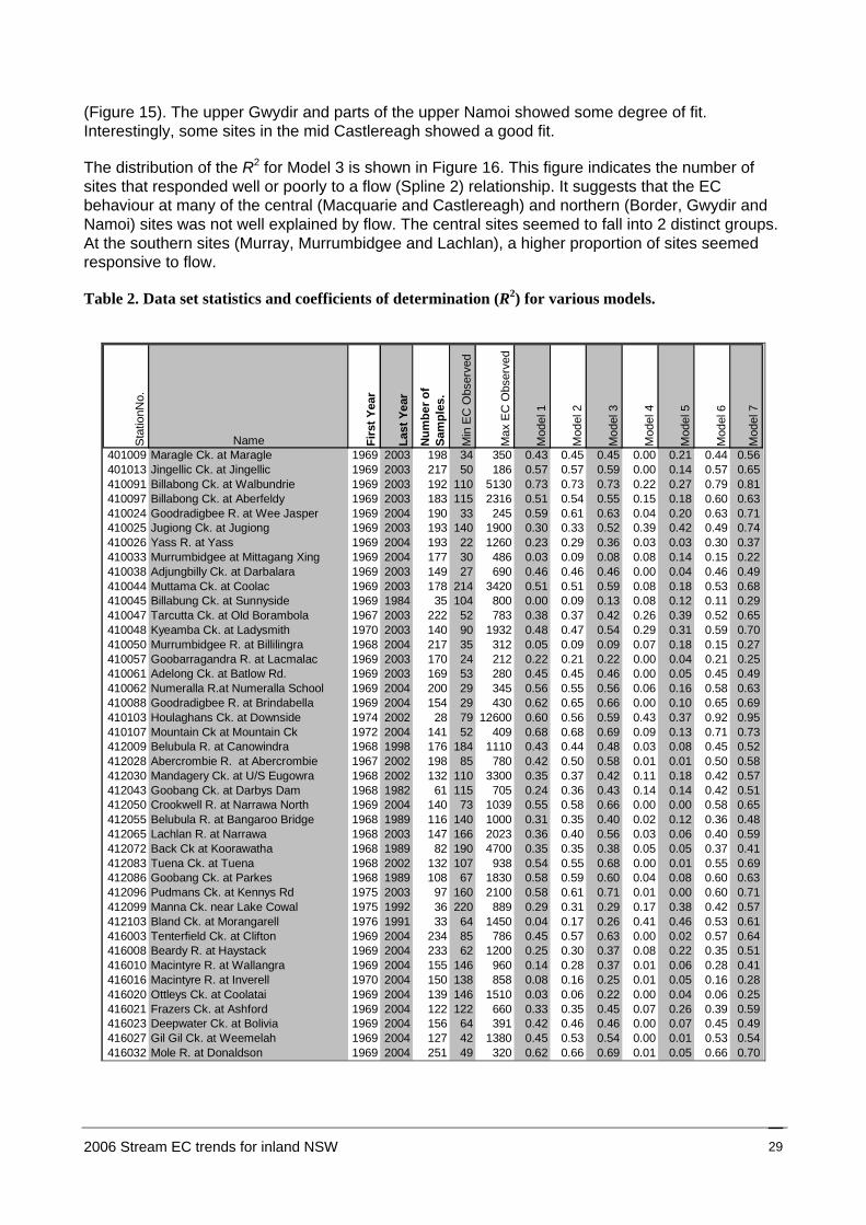
(Figure 15). The upper Gwydir and parts of the upper Namoi showed some degree of fit. Interestingly, some sites in the mid Castlereagh showed a good fit.
The distribution of the R2 for Model 3 is shown in Figure 16. This figure indicates the number of sites that responded well or poorly to a flow (Spline 2) relationship. It suggests that the EC behaviour at many of the central (Macquarie and Castlereagh) and northern (Border, Gwydir and Namoi) sites was not well explained by flow. The central sites seemed to fall into 2 distinct groups. At the southern sites (Murray, Murrumbidgee and Lachlan), a higher proportion of sites seemed responsive to flow.
Table 2. Data set statistics and coefficients of determination (R2) for various models.
Stat
ionN
o.
Name Firs
t Yea
r
Last
Yea
r
Num
ber o
f Sa
mpl
es.
Min
EC
Obs
erve
d
Max
EC
Obs
erve
d
Mod
el 1
Mod
el 2
Mod
el 3
Mod
el 4
Mod
el 5
Mod
el 6
Mod
el 7
401009 Maragle Ck. at Maragle 1969 2003 198 34 350 0.43 0.45 0.45 0.00 0.21 0.44 0.56401013 Jingellic Ck. at Jingellic 1969 2003 217 50 186 0.57 0.57 0.59 0.00 0.14 0.57 0.65410091 Billabong Ck. at Walbundrie 1969 2003 192 110 5130 0.73 0.73 0.73 0.22 0.27 0.79 0.81410097 Billabong Ck. at Aberfeldy 1969 2003 183 115 2316 0.51 0.54 0.55 0.15 0.18 0.60 0.63410024 Goodradigbee R. at Wee Jasper 1969 2004 190 33 245 0.59 0.61 0.63 0.04 0.20 0.63 0.71410025 Jugiong Ck. at Jugiong 1969 2003 193 140 1900 0.30 0.33 0.52 0.39 0.42 0.49 0.74410026 Yass R. at Yass 1969 2004 193 22 1260 0.23 0.29 0.36 0.03 0.03 0.30 0.37410033 Murrumbidgee at Mittagang Xing 1969 2004 177 30 486 0.03 0.09 0.08 0.08 0.14 0.15 0.22410038 Adjungbilly Ck. at Darbalara 1969 2003 149 27 690 0.46 0.46 0.46 0.00 0.04 0.46 0.49410044 Muttama Ck. at Coolac 1969 2003 178 214 3420 0.51 0.51 0.59 0.08 0.18 0.53 0.68410045 Billabung Ck. at Sunnyside 1969 1984 35 104 800 0.00 0.09 0.13 0.08 0.12 0.11 0.29410047 Tarcutta Ck. at Old Borambola 1967 2003 222 52 783 0.38 0.37 0.42 0.26 0.39 0.52 0.65410048 Kyeamba Ck. at Ladysmith 1970 2003 140 90 1932 0.48 0.47 0.54 0.29 0.31 0.59 0.70410050 Murrumbidgee R. at Billilingra 1968 2004 217 35 312 0.05 0.09 0.09 0.07 0.18 0.15 0.27410057 Goobarragandra R. at Lacmalac 1969 2003 170 24 212 0.22 0.21 0.22 0.00 0.04 0.21 0.25410061 Adelong Ck. at Batlow Rd. 1969 2003 169 53 280 0.45 0.45 0.46 0.00 0.05 0.45 0.49410062 Numeralla R.at Numeralla School 1969 2004 200 29 345 0.56 0.55 0.56 0.06 0.16 0.58 0.63410088 Goodradigbee R. at Brindabella 1969 2004 154 29 430 0.62 0.65 0.66 0.00 0.10 0.65 0.69410103 Houlaghans Ck. at Downside 1974 2002 28 79 12600 0.60 0.56 0.59 0.43 0.37 0.92 0.95410107 Mountain Ck at Mountain Ck 1972 2004 141 52 409 0.68 0.68 0.69 0.09 0.13 0.71 0.73412009 Belubula R. at Canowindra 1968 1998 176 184 1110 0.43 0.44 0.48 0.03 0.08 0.45 0.52412028 Abercrombie R. at Abercrombie 1967 2002 198 85 780 0.42 0.50 0.58 0.01 0.01 0.50 0.58412030 Mandagery Ck. at U/S Eugowra 1968 2002 132 110 3300 0.35 0.37 0.42 0.11 0.18 0.42 0.57412043 Goobang Ck. at Darbys Dam 1968 1982 61 115 705 0.24 0.36 0.43 0.14 0.14 0.42 0.51412050 Crookwell R. at Narrawa North 1969 2004 140 73 1039 0.55 0.58 0.66 0.00 0.00 0.58 0.65412055 Belubula R. at Bangaroo Bridge 1968 1989 116 140 1000 0.31 0.35 0.40 0.02 0.12 0.36 0.48412065 Lachlan R. at Narrawa 1968 2003 147 166 2023 0.36 0.40 0.56 0.03 0.06 0.40 0.59412072 Back Ck at Koorawatha 1968 1989 82 190 4700 0.35 0.35 0.38 0.05 0.05 0.37 0.41412083 Tuena Ck. at Tuena 1968 2002 132 107 938 0.54 0.55 0.68 0.00 0.01 0.55 0.69412086 Goobang Ck. at Parkes 1968 1989 108 67 1830 0.58 0.59 0.60 0.04 0.08 0.60 0.63412096 Pudmans Ck. at Kennys Rd 1975 2003 97 160 2100 0.58 0.61 0.71 0.01 0.00 0.60 0.71412099 Manna Ck. near Lake Cowal 1975 1992 36 220 889 0.29 0.31 0.29 0.17 0.38 0.42 0.57412103 Bland Ck. at Morangarell 1976 1991 33 64 1450 0.04 0.17 0.26 0.41 0.46 0.53 0.61416003 Tenterfield Ck. at Clifton 1969 2004 234 85 786 0.45 0.57 0.63 0.00 0.02 0.57 0.64416008 Beardy R. at Haystack 1969 2004 233 62 1200 0.25 0.30 0.37 0.08 0.22 0.35 0.51416010 Macintyre R. at Wallangra 1969 2004 155 146 960 0.14 0.28 0.37 0.01 0.06 0.28 0.41416016 Macintyre R. at Inverell 1970 2004 150 138 858 0.08 0.16 0.25 0.01 0.05 0.16 0.28416020 Ottleys Ck. at Coolatai 1969 2004 139 146 1510 0.03 0.06 0.22 0.00 0.04 0.06 0.25416021 Frazers Ck. at Ashford 1969 2004 122 122 660 0.33 0.35 0.45 0.07 0.26 0.39 0.59416023 Deepwater Ck. at Bolivia 1969 2004 156 64 391 0.42 0.46 0.46 0.00 0.07 0.45 0.49416027 Gil Gil Ck. at Weemelah 1969 2004 127 42 1380 0.45 0.53 0.54 0.00 0.01 0.53 0.54416032 Mole R. at Donaldson 1969 2004 251 49 320 0.62 0.66 0.69 0.01 0.05 0.66 0.70
2006 Stream EC trends for inland NSW 29
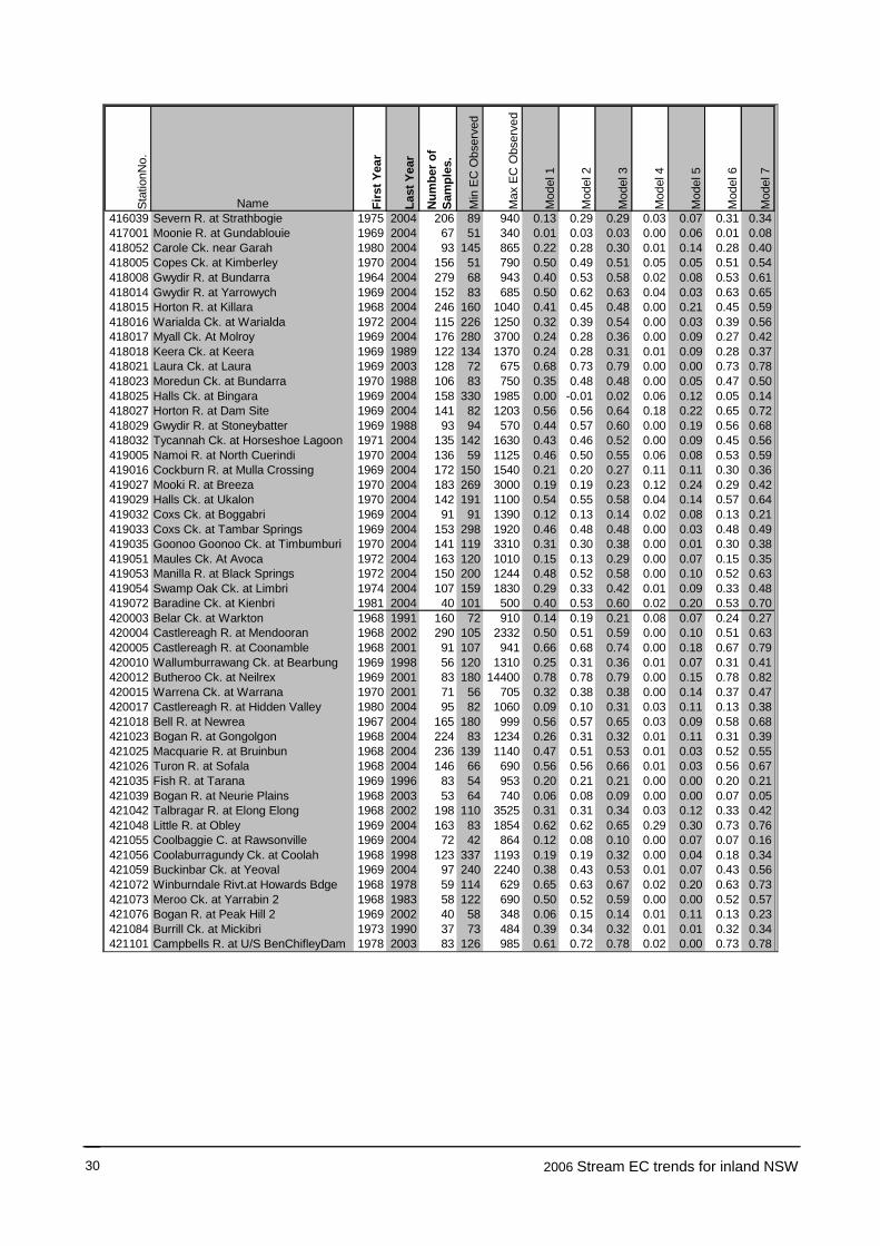
Stat
ionN
o.
Name Firs
t Yea
r
Last
Yea
r
Num
ber o
f Sa
mpl
es.
Min
EC
Obs
erve
d
Max
EC
Obs
erve
d
Mod
el 1
Mod
el 2
Mod
el 3
Mod
el 4
Mod
el 5
Mod
el 6
Mod
el 7
416039 Severn R. at Strathbogie 1975 2004 206 89 940 0.13 0.29 0.29 0.03 0.07 0.31 0.34417001 Moonie R. at Gundablouie 1969 2004 67 51 340 0.01 0.03 0.03 0.00 0.06 0.01 0.08418052 Carole Ck. near Garah 1980 2004 93 145 865 0.22 0.28 0.30 0.01 0.14 0.28 0.40418005 Copes Ck. at Kimberley 1970 2004 156 51 790 0.50 0.49 0.51 0.05 0.05 0.51 0.54418008 Gwydir R. at Bundarra 1964 2004 279 68 943 0.40 0.53 0.58 0.02 0.08 0.53 0.61418014 Gwydir R. at Yarrowych 1969 2004 152 83 685 0.50 0.62 0.63 0.04 0.03 0.63 0.65418015 Horton R. at Killara 1968 2004 246 160 1040 0.41 0.45 0.48 0.00 0.21 0.45 0.59418016 Warialda Ck. at Warialda 1972 2004 115 226 1250 0.32 0.39 0.54 0.00 0.03 0.39 0.56418017 Myall Ck. At Molroy 1969 2004 176 280 3700 0.24 0.28 0.36 0.00 0.09 0.27 0.42418018 Keera Ck. at Keera 1969 1989 122 134 1370 0.24 0.28 0.31 0.01 0.09 0.28 0.37418021 Laura Ck. at Laura 1969 2003 128 72 675 0.68 0.73 0.79 0.00 0.00 0.73 0.78418023 Moredun Ck. at Bundarra 1970 1988 106 83 750 0.35 0.48 0.48 0.00 0.05 0.47 0.50418025 Halls Ck. at Bingara 1969 2004 158 330 1985 0.00 -0.01 0.02 0.06 0.12 0.05 0.14418027 Horton R. at Dam Site 1969 2004 141 82 1203 0.56 0.56 0.64 0.18 0.22 0.65 0.72418029 Gwydir R. at Stoneybatter 1969 1988 93 94 570 0.44 0.57 0.60 0.00 0.19 0.56 0.68418032 Tycannah Ck. at Horseshoe Lagoon 1971 2004 135 142 1630 0.43 0.46 0.52 0.00 0.09 0.45 0.56419005 Namoi R. at North Cuerindi 1970 2004 136 59 1125 0.46 0.50 0.55 0.06 0.08 0.53 0.59419016 Cockburn R. at Mulla Crossing 1969 2004 172 150 1540 0.21 0.20 0.27 0.11 0.11 0.30 0.36419027 Mooki R. at Breeza 1970 2004 183 269 3000 0.19 0.19 0.23 0.12 0.24 0.29 0.42419029 Halls Ck. at Ukalon 1970 2004 142 191 1100 0.54 0.55 0.58 0.04 0.14 0.57 0.64419032 Coxs Ck. at Boggabri 1969 2004 91 91 1390 0.12 0.13 0.14 0.02 0.08 0.13 0.21419033 Coxs Ck. at Tambar Springs 1969 2004 153 298 1920 0.46 0.48 0.48 0.00 0.03 0.48 0.49419035 Goonoo Goonoo Ck. at Timbumburi 1970 2004 141 119 3310 0.31 0.30 0.38 0.00 0.01 0.30 0.38419051 Maules Ck. At Avoca 1972 2004 163 120 1010 0.15 0.13 0.29 0.00 0.07 0.15 0.35419053 Manilla R. at Black Springs 1972 2004 150 200 1244 0.48 0.52 0.58 0.00 0.10 0.52 0.63419054 Swamp Oak Ck. at Limbri 1974 2004 107 159 1830 0.29 0.33 0.42 0.01 0.09 0.33 0.48419072 Baradine Ck. at Kienbri 1981 2004 40 101 500 0.40 0.53 0.60 0.02 0.20 0.53 0.70420003 Belar Ck. at Warkton 1968 1991 160 72 910 0.14 0.19 0.21 0.08 0.07 0.24 0.27420004 Castlereagh R. at Mendooran 1968 2002 290 105 2332 0.50 0.51 0.59 0.00 0.10 0.51 0.63420005 Castlereagh R. at Coonamble 1968 2001 91 107 941 0.66 0.68 0.74 0.00 0.18 0.67 0.79420010 Wallumburrawang Ck. at Bearbung 1969 1998 56 120 1310 0.25 0.31 0.36 0.01 0.07 0.31 0.41420012 Butheroo Ck. at Neilrex 1969 2001 83 180 14400 0.78 0.78 0.79 0.00 0.15 0.78 0.82420015 Warrena Ck. at Warrana 1970 2001 71 56 705 0.32 0.38 0.38 0.00 0.14 0.37 0.47420017 Castlereagh R. at Hidden Valley 1980 2004 95 82 1060 0.09 0.10 0.31 0.03 0.11 0.13 0.38421018 Bell R. at Newrea 1967 2004 165 180 999 0.56 0.57 0.65 0.03 0.09 0.58 0.68421023 Bogan R. at Gongolgon 1968 2004 224 83 1234 0.26 0.31 0.32 0.01 0.11 0.31 0.39421025 Macquarie R. at Bruinbun 1968 2004 236 139 1140 0.47 0.51 0.53 0.01 0.03 0.52 0.55421026 Turon R. at Sofala 1968 2004 146 66 690 0.56 0.56 0.66 0.01 0.03 0.56 0.67421035 Fish R. at Tarana 1969 1996 83 54 953 0.20 0.21 0.21 0.00 0.00 0.20 0.21421039 Bogan R. at Neurie Plains 1968 2003 53 64 740 0.06 0.08 0.09 0.00 0.00 0.07 0.05421042 Talbragar R. at Elong Elong 1968 2002 198 110 3525 0.31 0.31 0.34 0.03 0.12 0.33 0.42421048 Little R. at Obley 1969 2004 163 83 1854 0.62 0.62 0.65 0.29 0.30 0.73 0.76421055 Coolbaggie C. at Rawsonville 1969 2004 72 42 864 0.12 0.08 0.10 0.00 0.07 0.07 0.16421056 Coolaburragundy Ck. at Coolah 1968 1998 123 337 1193 0.19 0.19 0.32 0.00 0.04 0.18 0.34421059 Buckinbar Ck. at Yeoval 1969 2004 97 240 2240 0.38 0.43 0.53 0.01 0.07 0.43 0.56421072 Winburndale Rivt.at Howards Bdge 1968 1978 59 114 629 0.65 0.63 0.67 0.02 0.20 0.63 0.73421073 Meroo Ck. at Yarrabin 2 1968 1983 58 122 690 0.50 0.52 0.59 0.00 0.00 0.52 0.57421076 Bogan R. at Peak Hill 2 1969 2002 40 58 348 0.06 0.15 0.14 0.01 0.11 0.13 0.23421084 Burrill Ck. at Mickibri 1973 1990 37 73 484 0.39 0.34 0.32 0.01 0.01 0.32 0.34421101 Campbells R. at U/S BenChifleyDam 1978 2003 83 126 985 0.61 0.72 0.78 0.02 0.00 0.73 0.78
2006 Stream EC trends for inland NSW 30

Figure 14. Map showing performance of Model 3, southern NSW.
EC as modelled by ‘short-term’ influences (flow spline and seasonality).
2006 Stream EC trends for inland NSW 31
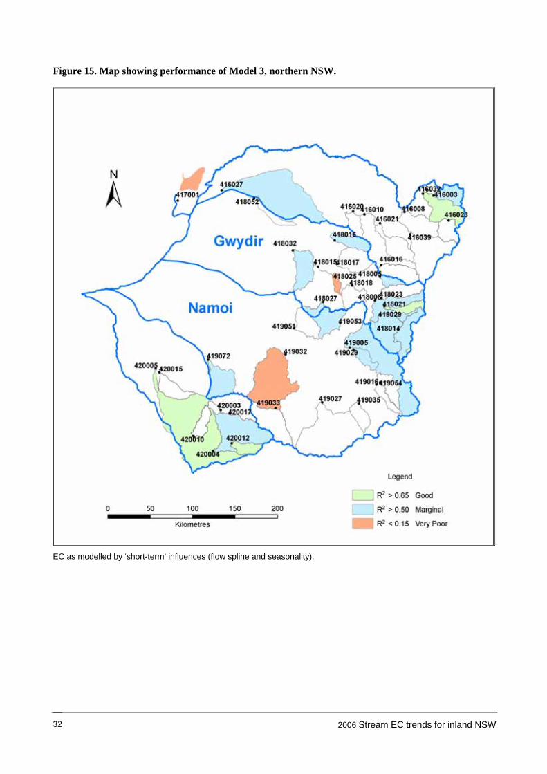
Figure 15. Map showing performance of Model 3, northern NSW.
EC as modelled by ‘short-term’ influences (flow spline and seasonality).
2006 Stream EC trends for inland NSW 32

Figure 16. Model 3, distribution of R2 across NSW.
5.1.3 Time as a descriptor of EC (Model 5)
Of the 2 models that attempted to fit time to flow-adjusted EC, the spline function of time (Model 5) showed the highest degree of predictive power. Its purpose was to evaluate whether the flow-adjusted EC data set showed any non-linear time trend. At some sites (mainly in the south), the spline time component (Model 5) had a substantial effect (Figures 17 and 18). R2 was ≥ 0.3 and was considered a substantial response for Model 5, and occurred at the following sites:
410025 Jugiong Creek at Jugiong
410047 Tarcutta Creek at Old Borambola
410048 Kyeamba Creek at Ladysmith
410103 Houlaghans Creek at Downside
412099 Manna Creek Nr Lake Cowal
412103 Bland Creek at Morangarell
421048 Little River at Obley
2006 Stream EC trends for inland NSW 33
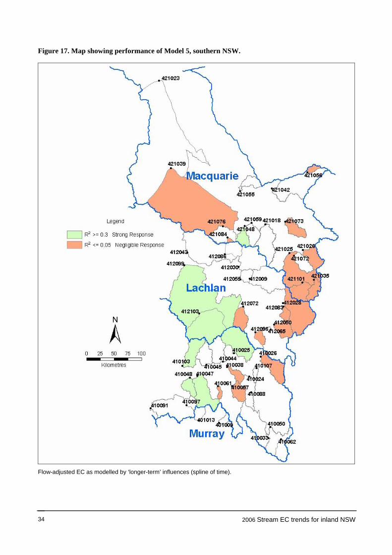
Figure 17. Map showing performance of Model 5, southern NSW.
Flow-adjusted EC as modelled by ‘longer-term’ influences (spline of time).
2006 Stream EC trends for inland NSW 34

All sites except 421048 are located in the central Murrumbidgee–Lachlan. At most other sites, the additional effect of time as an explanatory variable was far less marked. At 27 of the 92 sites, Table 2 suggests that EC trends are small or negligible over time (Model 5, R2 ≤ 0.05). Figure 17 and (to a much lesser extent) Figure 18 suggests that the catchments where Model 5 showed some significance had low-elevation outlets. The catchments where Model 5 had little influence were generally of a high elevation, i.e. at the top of the valleys. Figure 19 shows the distribution of the Model 5 performance across NSW, and suggests that the 3 northern valleys have a large proportion of the ‘non-respondents’ to Model 5.
Figure 18. Map showing performance of Model 5, northern NSW.
Flow-adjusted EC as modelled by ‘longer-term’ influences (spline of time).
2006 Stream EC trends for inland NSW 35

Figure 19. Model 5, distribution of R2 across NSW.
5.1.4 Performance of the full GAM (Model 7)
Interest focused on the full and more complex Model 7, since it generally provided the best fit to the EC data (Table 2). However, R2 can be misleading if used as the sole indicator of a model’s performance. For example, 410103 Houlaghans Creek at Downside, with just 28 data values spanning 28 years, shows a high final R2 of 0.95. In fact, the deviations from the fitted curve are large, but small when compared with the huge influence of the trend component (Model 5) at the site. At some other sites, such as 410038 Adjungbilly Creek at Darbalara, the trend component is minor, but R2 is as low as 0.49. Here, the limitations of data collection instruments are likely to have a much larger impact than any fitted trend. Thus, we have much more confidence in the Adjungbilly Creek trend results than in the Houlaghans Creek results.
Despite those reservations, the distribution of the set of Model 7 R2 values is presented spatially (Figures 20 and 21) and as histograms (Figure 22).
2006 Stream EC trends for inland NSW 36

Figure 20. Map showing performance of Model 7, southern half of NSW.
EC as modelled by combining ‘short-term’ and ‘longer-term’ influences.
2006 Stream EC trends for inland NSW 37

Figure 21. Map showing performance of Model 7, northern half of NSW.
EC as modelled by combining ‘short-term’ and ‘longer-term’ influences.
2006 Stream EC trends for inland NSW 38

Figure 22. Model 7, distribution of R2 across NSW.
An arbitrary decision was made to use R2 ≥ 0.65 as indicating a successful Model 7 fit. Under this criterion, a site was considered adequately modelled if 2/3 of the variance in EC could be explained by Model 7. There were 25 sites in this category, 13 of them in the 3 southern-most valleys. The R2 values for a further 8 sites fell between 0.6 and 0.65 and were categorised as ‘marginal’. Model 7 generated a larger number of high R2 values in the south of the State than in the north. This success was probably driven by the comparatively large trend component (Model 5) at a number of the southern sites (Figures 17, 19). Also worthy of note was the spatial grouping of the Macquarie Valley, in which the better Model 7 performers clustered in the south-east of the valley. In summary, the better results of Model 7 were obtained in the upper valleys of the Gwydir, Macquarie, Lachlan and generally scattered throughout the Murrumbidgee.
A ‘very poor’ category was established for sites with Model 7 R2 < 0.3. For these, we concluded that the combination of flow and time trend components was poor at explaining the variation in EC data. There were 14 such sites throughout the State.
5.1.5 Link between Model 3 and Model 7
Model 7 combined flow and time components to predict EC. It was of interest to note the difference in magnitude of the R2 values between Models 7 and 3, as the models differ in the inclusion of the spline time component (Model 5). Only at the few sites listed in Section 5.1.3 did the time spline function (as calculated in Model 5) appear to contribute beneficially to Model 7. Of flow and time, flow appears to be a stronger contributor to Model 7 performance. To explore this link, the R2 of
2006 Stream EC trends for inland NSW 39

Model 3 is plotted against the Model 7 R2 (Figures 23, 24). The red line is a smoothed line of best fit and the blue is a one-to-one line.
Figure 23. Plot of Model 3 R2 vs Model 7 final R2 in all central and northern valleys.
Figures 23 and 24 indicate that the performance of the more complex Model 7 seems to be only marginally better than that of Model 3 in the north of the State. This should be seen in the context that, generally, the models did not perform as well in the north and centre of the State. In the south, there appeared to be much less of a clear link (less duplication) between Models 3 and 7, i.e. Model 7 is an improvement over Model 3 owing to the added time spline. As flagged in Section 5.1.3 and Table 2, the time component plays an additional influential role (over and above that of flow) at the listed sites. This is borne out by some of the relatively high R2 values for Model 5 (already discussed in Section 5.1.3).
2006 Stream EC trends for inland NSW 40
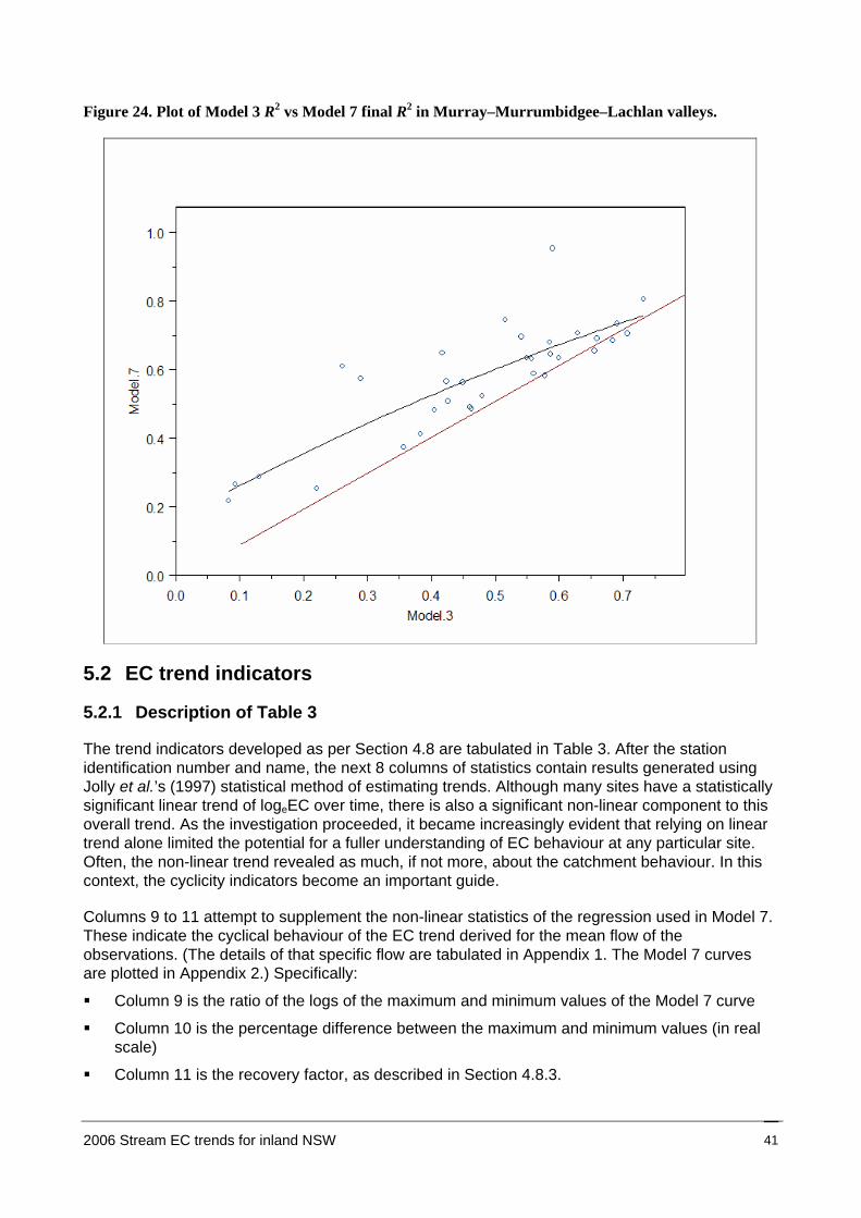
Figure 24. Plot of Model 3 R2 vs Model 7 final R2 in Murray–Murrumbidgee–Lachlan valleys.
5.2 EC trend indicators
5.2.1 Description of Table 3
The trend indicators developed as per Section 4.8 are tabulated in Table 3. After the station identification number and name, the next 8 columns of statistics contain results generated using Jolly et al.’s (1997) statistical method of estimating trends. Although many sites have a statistically significant linear trend of logeEC over time, there is also a significant non-linear component to this overall trend. As the investigation proceeded, it became increasingly evident that relying on linear trend alone limited the potential for a fuller understanding of EC behaviour at any particular site. Often, the non-linear trend revealed as much, if not more, about the catchment behaviour. In this context, the cyclicity indicators become an important guide.
Columns 9 to 11 attempt to supplement the non-linear statistics of the regression used in Model 7. These indicate the cyclical behaviour of the EC trend derived for the mean flow of the observations. (The details of that specific flow are tabulated in Appendix 1. The Model 7 curves are plotted in Appendix 2.) Specifically:
Column 9 is the ratio of the logs of the maximum and minimum values of the Model 7 curve
Column 10 is the percentage difference between the maximum and minimum values (in real scale)
Column 11 is the recovery factor, as described in Section 4.8.3.
2006 Stream EC trends for inland NSW 41

42
The graphs in Appendix 2 show that the recovery factor method (Section 4.8.3) was a good indicator of the trend in the Murrumbidgee–Murray (station numbers 409--- and 410---). At many sites in these valleys, the EC had been steadily rising since the start of the record, and showed signs of stabilising only in the mid 1990s. The recovery factor (section 4.8.3) was not a useful tool in the north, where many of the stations showed completely different behaviour, starting with a falling trend and then beginning to rise. When applied to the northern valleys, it ignored the trough. Consequently, the calculation could not effectively indicate the catchment’s capacity to drop back to low EC levels.
The large percentages (in Column 10) at some of the sites indicate large cyclic fluctuations. The magnitudes of these cycles stress the danger of calculating EC trends or attempting to provide forecasts for 2020.
2006 Stream EC trends for inland NSW
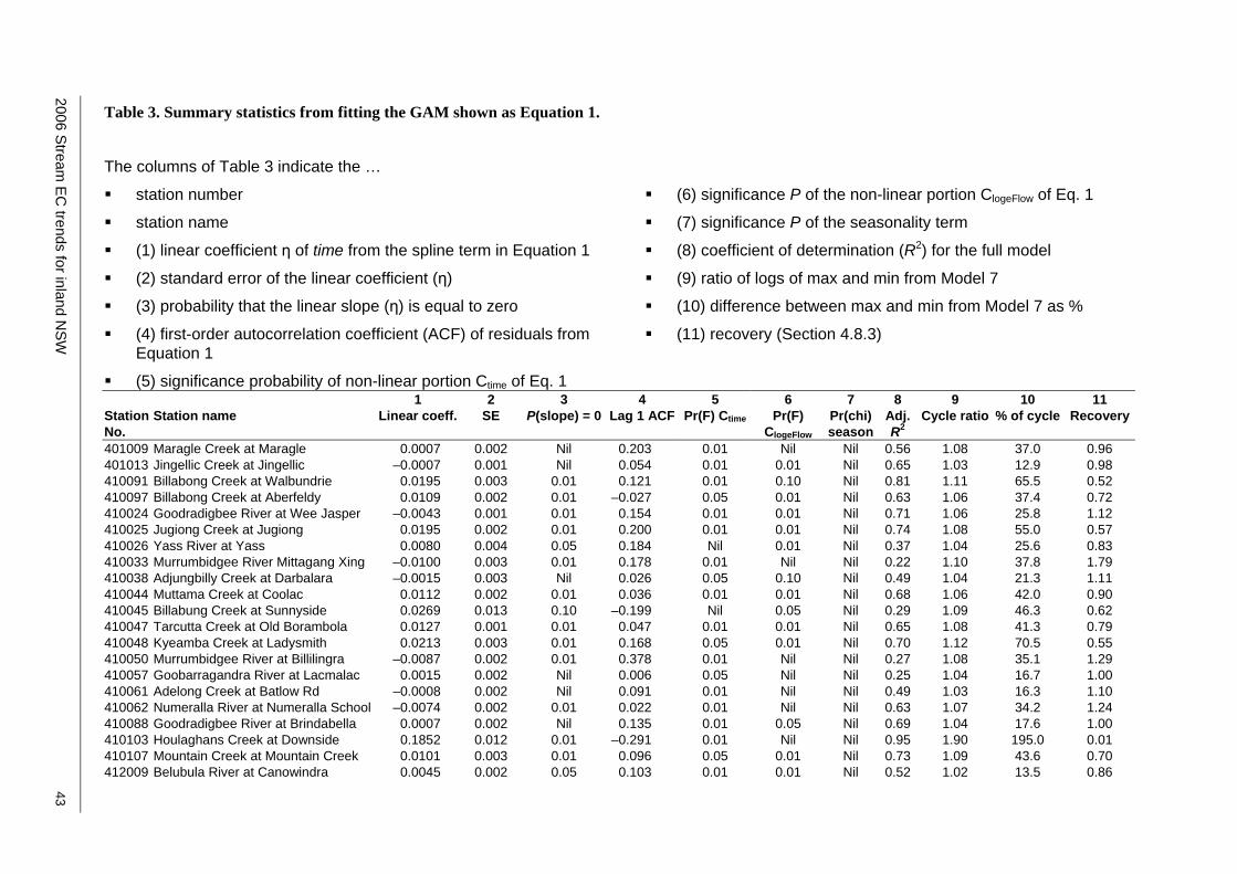
2006 Stream
EC
trends for inland NSW
43
Table 3. Summary statistics from fitting the GAM shown as Equation 1.
The columns of Table 3 indicate the …
station number
station name
(1) linear coefficient η of time from the spline term in Equation 1
(2) standard error of the linear coefficient (η)
(3) probability that the linear slope (η) is equal to zero
(4) first-order autocorrelation coefficient (ACF) of residuals from Equation 1
(5) significance probability of non-linear portion Ctime of Eq. 1
(6) significance P of the non-linear portion ClogeFlow of Eq. 1
(7) significance P of the seasonality term
(8) coefficient of determination (R2) for the full model
(9) ratio of logs of max and min from Model 7
(10) difference between max and min from Model 7 as %
(11) recovery (Section 4.8.3)
1 2 3 4 5 6 7 8 9 10 11 Station No.
Station name Linear coeff. SE P(slope) = 0 Lag 1 ACF Pr(F) Ctime Pr(F) ClogeFlow
Pr(chi) season
Adj. R2
Cycle ratio % of cycle Recovery
401009 Maragle Creek at Maragle 0.0007 0.002 Nil 0.203 0.01 Nil Nil 0.56 1.08 37.0 0.96 401013 Jingellic Creek at Jingellic –0.0007 0.001 Nil 0.054 0.01 0.01 Nil 0.65 1.03 12.9 0.98 410091 Billabong Creek at Walbundrie 0.0195 0.003 0.01 0.121 0.01 0.10 Nil 0.81 1.11 65.5 0.52 410097 Billabong Creek at Aberfeldy 0.0109 0.002 0.01 –0.027 0.05 0.01 Nil 0.63 1.06 37.4 0.72 410024 Goodradigbee River at Wee Jasper –0.0043 0.001 0.01 0.154 0.01 0.01 Nil 0.71 1.06 25.8 1.12 410025 Jugiong Creek at Jugiong 0.0195 0.002 0.01 0.200 0.01 0.01 Nil 0.74 1.08 55.0 0.57 410026 Yass River at Yass 0.0080 0.004 0.05 0.184 Nil 0.01 Nil 0.37 1.04 25.6 0.83 410033 Murrumbidgee River Mittagang Xing –0.0100 0.003 0.01 0.178 0.01 Nil Nil 0.22 1.10 37.8 1.79 410038 Adjungbilly Creek at Darbalara –0.0015 0.003 Nil 0.026 0.05 0.10 Nil 0.49 1.04 21.3 1.11 410044 Muttama Creek at Coolac 0.0112 0.002 0.01 0.036 0.01 0.01 Nil 0.68 1.06 42.0 0.90 410045 Billabung Creek at Sunnyside 0.0269 0.013 0.10 –0.199 Nil 0.05 Nil 0.29 1.09 46.3 0.62 410047 Tarcutta Creek at Old Borambola 0.0127 0.001 0.01 0.047 0.01 0.01 Nil 0.65 1.08 41.3 0.79 410048 Kyeamba Creek at Ladysmith 0.0213 0.003 0.01 0.168 0.05 0.01 Nil 0.70 1.12 70.5 0.55 410050 Murrumbidgee River at Billilingra –0.0087 0.002 0.01 0.378 0.01 Nil Nil 0.27 1.08 35.1 1.29 410057 Goobarragandra River at Lacmalac 0.0015 0.002 Nil 0.006 0.05 Nil Nil 0.25 1.04 16.7 1.00 410061 Adelong Creek at Batlow Rd –0.0008 0.002 Nil 0.091 0.01 Nil Nil 0.49 1.03 16.3 1.10 410062 Numeralla River at Numeralla School –0.0074 0.002 0.01 0.022 0.01 Nil Nil 0.63 1.07 34.2 1.24 410088 Goodradigbee River at Brindabella 0.0007 0.002 Nil 0.135 0.01 0.05 Nil 0.69 1.04 17.6 1.00 410103 Houlaghans Creek at Downside 0.1852 0.012 0.01 –0.291 0.01 Nil Nil 0.95 1.90 195.0 0.01 410107 Mountain Creek at Mountain Creek 0.0101 0.003 0.01 0.096 0.05 0.01 Nil 0.73 1.09 43.6 0.70 412009 Belubula River at Canowindra 0.0045 0.002 0.05 0.103 0.01 0.01 Nil 0.52 1.02 13.5 0.86
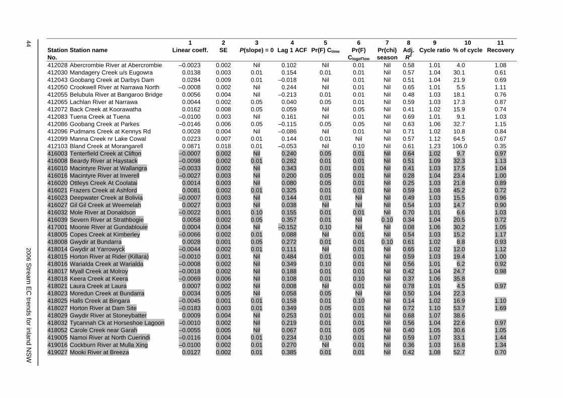
1 2 3 4 5 6 7 8 9 10 11
44 2006 S
tream E
C trends for inland N
SW
Station No.
Station name Linear coeff. SE P(slope) = 0 Lag 1 ACF Pr(F) Ctime Pr(F) ClogeFlow
Pr(chi) season
Adj. R2
Cycle ratio % of cycle Recovery
412028 Abercrombie River at Abercrombie –0.0023 0.002 Nil 0.102 Nil 0.01 Nil 0.58 1.01 4.0 1.08 412030 Mandagery Creek u/s Eugowra 0.0138 0.003 0.01 0.154 0.01 0.01 Nil 0.57 1.04 30.1 0.61 412043 Goobang Creek at Darbys Dam 0.0284 0.009 0.01 –0.018 Nil 0.01 Nil 0.51 1.04 21.9 0.69 412050 Crookwell River at Narrawa North –0.0008 0.002 Nil 0.244 Nil 0.01 Nil 0.65 1.01 5.5 1.11 412055 Belubula River at Bangaroo Bridge 0.0056 0.004 Nil –0.213 0.01 0.01 Nil 0.48 1.03 18.1 0.76 412065 Lachlan River at Narrawa 0.0044 0.002 0.05 0.040 0.05 0.01 Nil 0.59 1.03 17.3 0.87 412072 Back Creek at Koorawatha 0.0162 0.008 0.05 0.059 Nil 0.05 Nil 0.41 1.02 15.9 0.74 412083 Tuena Creek at Tuena –0.0100 0.003 Nil 0.161 Nil 0.01 Nil 0.69 1.01 9.1 1.03 412086 Goobang Creek at Parkes –0.0146 0.006 0.05 –0.115 0.05 0.05 Nil 0.63 1.06 32.7 1.15 412096 Pudmans Creek at Kennys Rd 0.0028 0.004 Nil –0.086 Nil 0.01 Nil 0.71 1.02 10.8 0.84 412099 Manna Creek nr Lake Cowal 0.0223 0.007 0.01 0.144 0.01 Nil Nil 0.57 1.12 64.5 0.67 412103 Bland Creek at Morangarell 0.0871 0.018 0.01 –0.053 Nil 0.10 Nil 0.61 1.23 106.0 0.35 416003 Tenterfield Creek at Clifton –0.0007 0.002 Nil 0.240 0.05 0.01 Nil 0.64 1.02 9.7 0.97 416008 Beardy River at Haystack –0.0098 0.002 0.01 0.282 0.01 0.01 Nil 0.51 1.09 32.3 1.13 416010 Macintyre River at Wallangra –0.0033 0.002 Nil 0.343 0.01 0.01 Nil 0.41 1.03 17.5 1.04 416016 Macintyre River at Inverell –0.0027 0.003 Nil 0.200 0.05 0.01 Nil 0.28 1.04 23.4 1.00 416020 Ottleys Creek At Coolatai 0.0014 0.003 Nil 0.080 0.05 0.01 Nil 0.25 1.03 21.8 0.89 416021 Frazers Creek at Ashford 0.0081 0.002 0.01 0.325 0.01 0.01 Nil 0.59 1.08 45.2 0.72 416023 Deepwater Creek at Bolivia –0.0007 0.003 Nil 0.144 0.01 Nil Nil 0.49 1.03 15.5 0.96 416027 Gil Gil Creek at Weemelah 0.0027 0.003 Nil 0.038 Nil Nil Nil 0.54 1.03 14.7 0.90 416032 Mole River at Donaldson –0.0022 0.001 0.10 0.155 0.01 0.01 Nil 0.70 1.01 6.6 1.03 416039 Severn River at Strathbogie 0.0058 0.002 0.05 0.357 0.01 Nil 0.10 0.34 1.04 20.5 0.72 417001 Moonie River at Gundablouie 0.0004 0.004 Nil –0.152 0.10 Nil Nil 0.08 1.06 30.2 1.05 418005 Copes Creek at Kimberley –0.0066 0.002 0.01 0.088 Nil 0.01 Nil 0.54 1.03 15.2 1.17 418008 Gwydir at Bundarra 0.0028 0.001 0.05 0.272 0.01 0.01 0.10 0.61 1.02 8.8 0.93 418014 Gwydir at Yarrowyck –0.0044 0.002 0.01 0.111 Nil 0.01 Nil 0.65 1.02 12.0 1.12 418015 Horton River at Rider (Killara) –0.0010 0.001 Nil 0.484 0.01 0.01 Nil 0.59 1.03 19.4 1.00 418016 Warialda Creek at Warialda –0.0008 0.002 Nil 0.349 0.10 0.01 Nil 0.56 1.01 6.2 0.92 418017 Myall Creek at Molroy –0.0018 0.002 Nil 0.188 0.01 0.01 Nil 0.42 1.04 24.7 0.98 418018 Keera Creek at Keera –0.0069 0.006 Nil 0.108 0.01 0.10 Nil 0.37 1.06 35.8 418021 Laura Creek at Laura 0.0007 0.002 Nil 0.008 Nil 0.01 Nil 0.78 1.01 4.5 0.97 418023 Moredun Creek at Bundarra 0.0034 0.005 Nil 0.058 0.05 Nil Nil 0.50 1.04 22.3 418025 Halls Creek at Bingara –0.0045 0.001 0.01 0.158 0.01 0.10 Nil 0.14 1.02 16.9 1.10 418027 Horton River at Dam Site –0.0183 0.003 0.01 0.349 0.05 0.01 Nil 0.72 1.10 53.7 1.69 418029 Gwydir River at Stoneybatter 0.0009 0.004 Nil 0.253 0.01 0.01 Nil 0.68 1.07 38.6 418032 Tycannah Ck at Horseshoe Lagoon –0.0010 0.002 Nil 0.219 0.01 0.01 Nil 0.56 1.04 22.6 0.97 418052 Carole Creek near Garah –0.0055 0.005 Nil 0.067 0.01 0.05 Nil 0.40 1.05 30.6 1.05 419005 Namoi River at North Cuerindi –0.0116 0.004 0.01 0.234 0.10 0.01 Nil 0.59 1.07 33.1 1.44 419016 Cockburn River at Mulla Xing –0.0100 0.002 0.01 0.270 Nil 0.01 Nil 0.36 1.03 16.8 1.34 419027 Mooki River at Breeza 0.0127 0.002 0.01 0.385 0.01 0.01 Nil 0.42 1.08 52.7 0.70
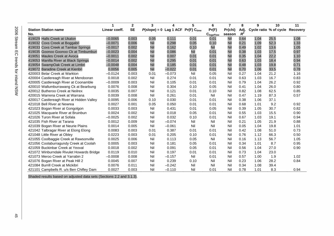
2006 Stream
EC
trends for inland NSW
45
1 2 3 4 5 6 7 8 9 10 11 Station No.
Station name Linear coeff. SE P(slope) = 0 Lag 1 ACF Pr(F) Ctime Pr(F) ClogeFlow
Pr(chi) season
Adj. R2
Cycle ratio % of cycle Recovery
419029 Halls Creek at Ukalon –0.0065 0.003 0.05 0.111 0.01 0.01 Nil 0.64 1.04 25.5 1.08 419032 Coxs Creek at Boggabri –0.0071 0.006 Nil 0.298 0.05 0.10 Nil 0.21 1.09 52.3 1.33 419033 Coxs Creek at Tambar Springs –0.0017 0.002 Nil 0.162 0.10 Nil Nil 0.49 1.02 13.6 1.05 419035 Goonoo Goonoo Ck at Timbumburi –0.0023 0.004 Nil 0.086 Nil 0.01 Nil 0.38 1.03 17.5 0.97 419051 Maules Creek at Avoca –0.0011 0.002 Nil 0.007 0.01 0.01 Nil 0.35 1.04 22.2 1.10 419053 Manilla River at Black Springs –0.0014 0.002 Nil 0.295 0.01 0.01 Nil 0.63 1.03 18.4 0.94 419054 SwampOak Creek at Limbri –0.0048 0.004 Nil 0.185 0.01 0.01 Nil 0.48 1.03 19.8 0.71 419072 Baradine Creek at Kienbri 0.0056 0.005 Nil –0.022 0.01 0.01 Nil 0.70 1.06 33.5 0.78 420003 Belar Creek at Warkton –0.0124 0.003 0.01 –0.073 Nil 0.05 Nil 0.27 1.04 21.2 1.16 420004 Castlereagh River at Mendooran 0.0018 0.002 Nil 0.274 0.01 0.01 Nil 0.63 1.03 16.7 0.83 420005 Castlereagh River at Coonamble –0.0009 0.003 Nil 0.105 0.01 0.01 Nil 0.79 1.04 26.2 0.92 420010 Wallumburrawang Ck at Bearbung 0.0076 0.008 Nil 0.304 0.10 0.05 Nil 0.41 1.04 26.0 0.80 420012 Butheroo Creek at Neilrex 0.0035 0.007 Nil 0.121 0.01 0.10 Nil 0.82 1.08 62.5 0.85 420015 Warrena Creek at Warrana 0.0039 0.008 Nil 0.261 0.01 Nil Nil 0.47 1.19 87.3 0.57 420017 Castlereagh River at Hidden Valley 0.0095 0.006 0.10 0.030 0.01 0.01 Nil 0.38 1.06 37.1 421018 Bell River at Newrea 0.0027 0.001 0.05 0.050 0.01 0.01 Nil 0.68 1.01 9.2 0.92 421023 Bogan River at Gongolgon 0.0033 0.003 Nil 0.431 0.01 0.05 Nil 0.39 1.05 30.7 0.82 421025 Macquarie River at Bruinbun 0.0024 0.002 Nil 0.018 0.05 0.01 Nil 0.55 1.03 15.5 0.90 421026 Turon River at Sofala –0.0025 0.002 Nil 0.032 0.10 0.01 Nil 0.67 1.03 19.1 0.94 421035 Fish River at Tarana 0.0012 0.009 Nil –0.074 Nil Nil Nil 0.21 1.05 21.9 0.88 421039 Bogan River at Neurie Plains 0.0014 0.005 Nil –0.061 Nil Nil Nil 0.05 1.04 19.8 1.01 421042 Talbragar River at Elong Elong 0.0083 0.003 0.01 0.387 0.01 0.01 Nil 0.42 1.08 51.0 0.73 421048 Little River at Obley 0.0223 0.003 0.01 0.205 0.10 0.01 Nil 0.76 1.12 66.3 0.50 421055 Coolbaggie Creek at Rawsonville 0.0025 0.006 Nil 0.113 0.05 Nil Nil 0.16 1.13 56.7 1.05 421056 Coolaburragundy Creek at Coolah 0.0005 0.003 Nil 0.181 0.05 0.01 Nil 0.34 1.01 8.7 0.95 421059 Buckinbar Creek at Yeoval 0.0018 0.002 Nil 0.091 0.05 0.01 Nil 0.56 1.04 27.0 0.90 421072 Winburndale Rivulet Howards Bridge 0.0119 0.010 Nil 0.197 0.01 0.01 Nil 0.73 1.04 23.0 421073 Meroo Creek at Yarrabin 2 –0.0008 0.008 Nil –0.157 Nil 0.01 Nil 0.57 1.00 1.9 1.02 421076 Bogan River at Peak Hill 2 0.0045 0.007 Nil 0.239 0.10 Nil Nil 0.23 1.06 28.2 0.84 421084 Burrill Creek at Mickibri 0.0076 0.011 Nil –0.242 Nil Nil Nil 0.34 1.08 39.4 421101 Campbells R. u/s Ben Chifley Dam 0.0027 0.003 Nil –0.110 Nil 0.01 Nil 0.78 1.01 8.3 0.94
Shaded results based on adjusted data sets (Sections 2.2 and 3.1.3).

5.2.2 Comparison of indicators
Three of the trend indicators described in Section 4.8 (statistical linearity, cycle ratio and percentage of cycle) have been plotted in Figure 25, using 90 of the 92 sites. Two sample points have been removed because we consider them to be outliers with an extreme influence on the projection of the fitted line. The sites, 410103 Houlaghans at Downside and 412103 Bland at Morangarell, are 2 of the more western catchments in the study area.
As might be expected, the cycle ratio and the percentage of cycle seem to be strongly linked (Figure 25). However, the 2 indicators based on cycle have no strong relationship with linear trend. There is a weak suggestion that the 2 cycle indicators increase as the magnitude of the linear trend increases (particularly when the linear trend is positive).
Figure 25. Matrix plot of 3 measures of trend.
Linear
1.00
1.05
1.10
1.15
1.20
-0.02 -0.01 0.00 0.01 0.02 0.03
1.00 1.05 1.10 1.15 1.20
Cycle.ratio
-0.02
-0.01
0.00
0.01
0.02
0.03
PctCycle
0
20
40
60
80
0 20 40 60 80
5.2.3 Other statistical measures of trend
Table 4 lists the significance of the linear (η) and non-linear (Ctime) time coefficients from Section 4.5. Over the period of observation, most sites exhibit non-linear curvature of their time response.
The proportional change in EC per year has been estimated using the equation eη – 1, which is then multiplied by the average EC (µS cm–1) over the period of observation to give an estimate of EC change in units of µS cm–1 y–1. This represents the annual average change in EC when the EC is at its average level. A 95% CI for this estimate has also been derived.
46 2006 Stream EC trends for inland NSW

Stream EC trends for inland NSW 2006 47
tn–2,0.05 is Student’s t statistic with n – 2 degrees of freedom.
SSx is the sums of squares of the observed time points
x is the mean of the observed time points
X is the time point at which the prediction is to be made
n is the number of observations used in the analysis
Section 8.9 discusses EC prediction to 2020. At those few sites that have a primarily linear time trend, the linear regression portion of the time trend can be used to fit confidence belts to the response curve using Equation 5. A tentative extrapolation may then be made to 2020. The calculation of these confidence belts is found in many text books on regression analysis:
Although prediction of future EC levels is extremely tentative, even when the response is strictly linear, prediction of mean % EC change from the first year of observation to 2020 cannot be estimated using this method in the presence of significant non-linear trend. Therefore, the final columns of Table 4 are given only for sites whose trend is primarily linear over the period of observation.
Each station’s predicted mean percentage change in EC over the period of observation (i.e. relative to that in the first year of observation), together with 95% CLs, is also listed in Table 4. Although this is an adequate measure of the linear compound change over the period of study, it is an inadequate indication of total change over the same period. For this reason, the significance of the non-linear time component affects the interpretation of these estimates of compound change.
s2 is the residual mean square derived from the data analysis
y is the estimated logeEC
where:
⎥⎦
⎤⎢⎣
⎡ −+∗± − SSx
xXn
sty n
22
05.0,2)(1ˆ (5)
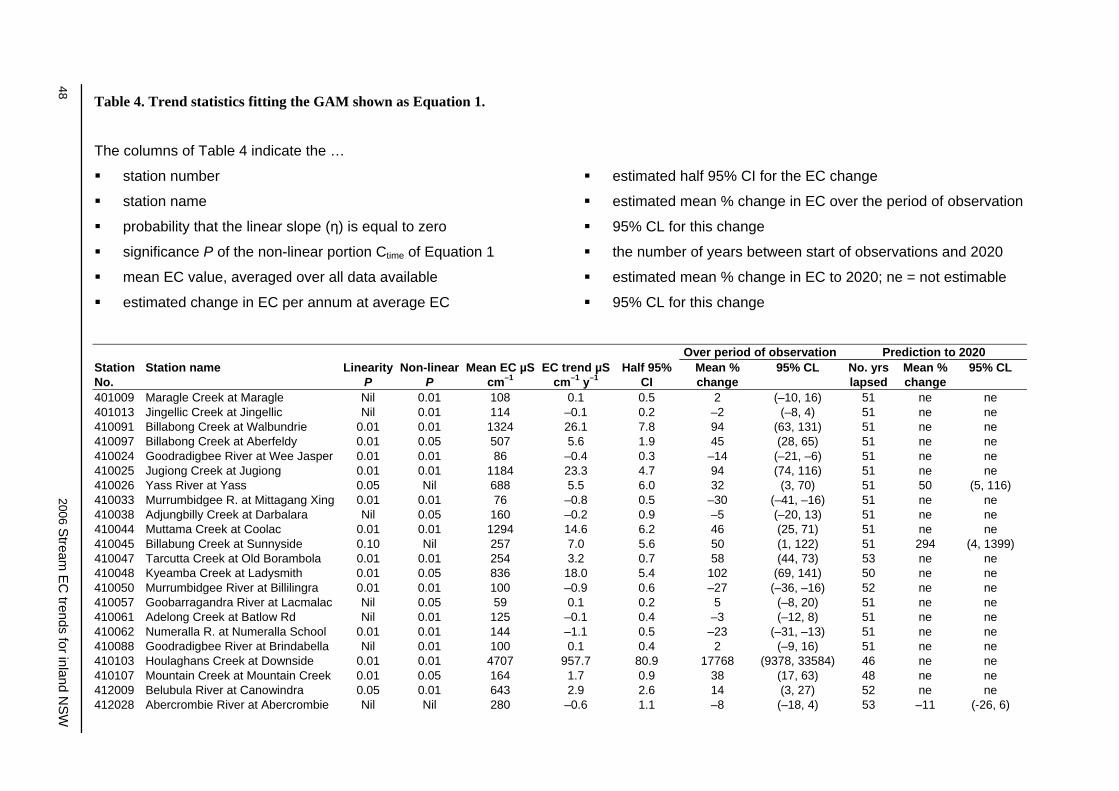
48 2006 S
tream E
C trends for inland N
SW
Table 4. Trend statistics fitting the GAM shown as Equation 1.
The columns of Table 4 indicate the …
station number
station name
probability that the linear slope (η) is equal to zero
significance P of the non-linear portion Ctime of Equation 1
mean EC value, averaged over all data available
estimated change in EC per annum at average EC
estimated half 95% CI for the EC change
estimated mean % change in EC over the period of observation
95% CL for this change
the number of years between start of observations and 2020
estimated mean % change in EC to 2020; ne = not estimable
95% CL for this change
Over period of observation Prediction to 2020 Station No.
Station name Linearity P
Non-linear P
Mean EC µS cm–1
EC trend µS cm–1 y–1
Half 95% CI
Mean % change
95% CL No. yrs lapsed
Mean % change
95% CL
401009 Maragle Creek at Maragle Nil 0.01 108 0.1 0.5 2 (–10, 16) 51 ne ne 401013 Jingellic Creek at Jingellic Nil 0.01 114 –0.1 0.2 –2 (–8, 4) 51 ne ne 410091 Billabong Creek at Walbundrie 0.01 0.01 1324 26.1 7.8 94 (63, 131) 51 ne ne 410097 Billabong Creek at Aberfeldy 0.01 0.05 507 5.6 1.9 45 (28, 65) 51 ne ne 410024 Goodradigbee River at Wee Jasper 0.01 0.01 86 –0.4 0.3 –14 (–21, –6) 51 ne ne 410025 Jugiong Creek at Jugiong 0.01 0.01 1184 23.3 4.7 94 (74, 116) 51 ne ne 410026 Yass River at Yass 0.05 Nil 688 5.5 6.0 32 (3, 70) 51 50 (5, 116) 410033 Murrumbidgee R. at Mittagang Xing 0.01 0.01 76 –0.8 0.5 –30 (–41, –16) 51 ne ne 410038 Adjungbilly Creek at Darbalara Nil 0.05 160 –0.2 0.9 –5 (–20, 13) 51 ne ne 410044 Muttama Creek at Coolac 0.01 0.01 1294 14.6 6.2 46 (25, 71) 51 ne ne 410045 Billabung Creek at Sunnyside 0.10 Nil 257 7.0 5.6 50 (1, 122) 51 294 (4, 1399) 410047 Tarcutta Creek at Old Borambola 0.01 0.01 254 3.2 0.7 58 (44, 73) 53 ne ne 410048 Kyeamba Creek at Ladysmith 0.01 0.05 836 18.0 5.4 102 (69, 141) 50 ne ne 410050 Murrumbidgee River at Billilingra 0.01 0.01 100 –0.9 0.6 –27 (–36, –16) 52 ne ne 410057 Goobarragandra River at Lacmalac Nil 0.05 59 0.1 0.2 5 (–8, 20) 51 ne ne 410061 Adelong Creek at Batlow Rd Nil 0.01 125 –0.1 0.4 –3 (–12, 8) 51 ne ne 410062 Numeralla R. at Numeralla School 0.01 0.01 144 –1.1 0.5 –23 (–31, –13) 51 ne ne 410088 Goodradigbee River at Brindabella Nil 0.01 100 0.1 0.4 2 (–9, 16) 51 ne ne 410103 Houlaghans Creek at Downside 0.01 0.01 4707 957.7 80.9 17768 (9378, 33584) 46 ne ne 410107 Mountain Creek at Mountain Creek 0.01 0.05 164 1.7 0.9 38 (17, 63) 48 ne ne 412009 Belubula River at Canowindra 0.05 0.01 643 2.9 2.6 14 (3, 27) 52 ne ne 412028 Abercrombie River at Abercrombie Nil Nil 280 –0.6 1.1 –8 (–18, 4) 53 –11 (-26, 6)

Over period of observation Prediction to 2020
2006 Stream
EC
trends for inland NSW
49
Station No.
Station name Linearity P
Non-linear P
Mean EC µS cm–1
EC trend µS cm–1 y–1
Half 95% CI
Mean % change
95% CL No. yrs lapsed
Mean % change
95% CL
412030 Mandagery Creek u/s Eugowra 0.01 0.01 987 13.7 7.4 60 (29, 98) 52 ne ne 412043 Goobang Creek at Darbys Dam 0.01 Nil 364 10.5 6.6 49 (15, 92) 52 338 (71, 1023) 412050 Crookwell River at Narrawa North Nil Nil 418 –0.3 2.3 –3 (–16, 12) 51 –4 (–22, 19) 412055 Belubula River at Bangaroo Bge Nil 0.01 624 3.5 4.0 12 (–5, 33) 52 ne ne 412065 Lachlan River at Narrawa 0.05 0.05 855 3.8 3.9 17 (0, 36) 52 ne ne 412072 Back Creek at Koorawatha 0.05 Nil 1665 27.2 28.1 41 (1, 95) 52 132 (3, 421) 412083 Tuena Creek at Tuena Nil Nil 483 –4.8 3.1 –29 (–41, –15) 52 –41 (–55, –22) 412086 Goobang Creek at Parkes 0.05 0.05 573 –8.3 6.6 –26 (–44, –4) 52 ne ne 412096 Pudmans Creek at Kennys Rd Nil Nil 1294 3.6 9.1 8 (–12, 33) 45 13 (–19, 59) 412099 Manna Creek near Lake Cowal 0.01 0.01 451 10.2 7.3 46 (16, 84) 45 ne ne 412103 Bland Creek at Morangarell 0.01 Nil 326 29.6 11.1 269 (120, 521) 44 4517 (905, 21113) 416003 Tenterfield Creek at Clifton Nil 0.05 332 –0.2 1.3 –2 (–12, 8) 51 ne ne 416008 Beardy River at Haystack 0.01 0.01 233 –2.3 1.3 –29 (–39, –18) 51 ne ne 416010 Macintyre River at Wallangra Nil 0.01 515 –1.7 3.4 –11 (–24, 4) 51 ne ne 416016 Macintyre River at Inverell Nil 0.05 493 –1.3 3.5 –9 (–25, 11) 50 ne ne 416020 Ottleys Creek at Coolatai Nil 0.05 724 1.0 4.2 5 (–13, 26) 51 ne ne 416021 Frazers Creek at Ashford 0.01 0.01 433 3.5 2.9 33 (13, 57) 51 ne ne 416023 Deepwater Creek at Bolivia Nil 0.01 159 –0.1 0.9 –2 (–18, 16) 51 ne ne 416027 Gil Gil Creek at Weemelah Nil Nil 420 1.1 2.9 10 (–12, 38) 51 15 (-18, 60) 416032 Mole River at Donaldson 0.10 0.01 204 –0.4 0.6 –7 (–15, 1) 51 ne ne 416039 Severn River at Strathbogie 0.05 0.01 298 1.7 2.0 18 (4, 35) 45 ne ne 417001 Moonie River at Gundablouie Nil 0.10 141 0.1 1.0 1 (–23, 34) 51 ne ne 418005 Copes Creek at Kimberley 0.01 Nil 178 –1.2 0.8 –20 (–31, –8) 50 –28 (–42, –12) 418008 Gwydir at Bundarra 0.05 0.01 284 0.8 0.9 12 (2, 23) 56 ne ne 418014 Gwydir at Yarrowyck 0.01 Nil 357 –1.6 1.4 –14 (–24, –4) 51 –20 (–33, –5) 418015 Horton River at Rider (Killara) Nil 0.01 622 –0.6 2.3 –4 (–11, 4) 52 ne ne 418016 Warialda Creek at Warialda Nil 0.10 833 –0.7 5.1 –3 (–15, 11) 48 ne ne 418017 Myall Creek at Molroy Nil 0.01 1046 –1.9 4.8 –6 (–18, 7) 51 ne ne 418018 Keera Creek at Keera Nil 0.01 611 –4.2 8.2 –13 (–31, 10) 51 ne ne 418021 Laura Creek at Laura Nil Nil 266 0.2 1.1 2 (–10, 17) 51 4 (–15, 27) 418023 Moredun Creek at Bundarra Nil 0.05 238 0.8 2.7 6 (–12, 28) 50 ne ne 418025 Halls Creek at Bingara 0.01 0.01 1039 –4.7 3.2 –15 (–22, –7) 51 ne ne 418027 Horton River at DamSite 0.01 0.05 506 –9.2 4.4 –47 (–57, –35) 51 ne ne 418029 Gwydir River at Stoneybatter Nil 0.01 301 0.3 3.0 2 (–12, 17) 51 ne ne 418032 Tycannah Ck at Horseshoe Lagoon Nil 0.01 749 –0.7 4.3 –3 (–17, 12) 49 ne ne 418052 Carole Creek near. Garah Nil 0.01 400 –2.2 4.1 –12 (–30, 10) 40 ne ne 419005 Namoi River at North Cuerindi 0.01 0.10 278 –3.2 2.7 –33 (–48, –13) 50 ne ne 419016 Cockburn River at Mulla Xing 0.01 Nil 434 –4.3 2.4 –30 (–39, –19) 51 -40 (–51, –26) 419027 Mooki River at Breeza 0.01 0.01 975 12.5 6.8 54 (32, 80) 50 ne ne 419029 Halls Creek at Ukalon 0.05 0.01 669 –4.3 3.7 –20 (–32, –5) 50 ne ne
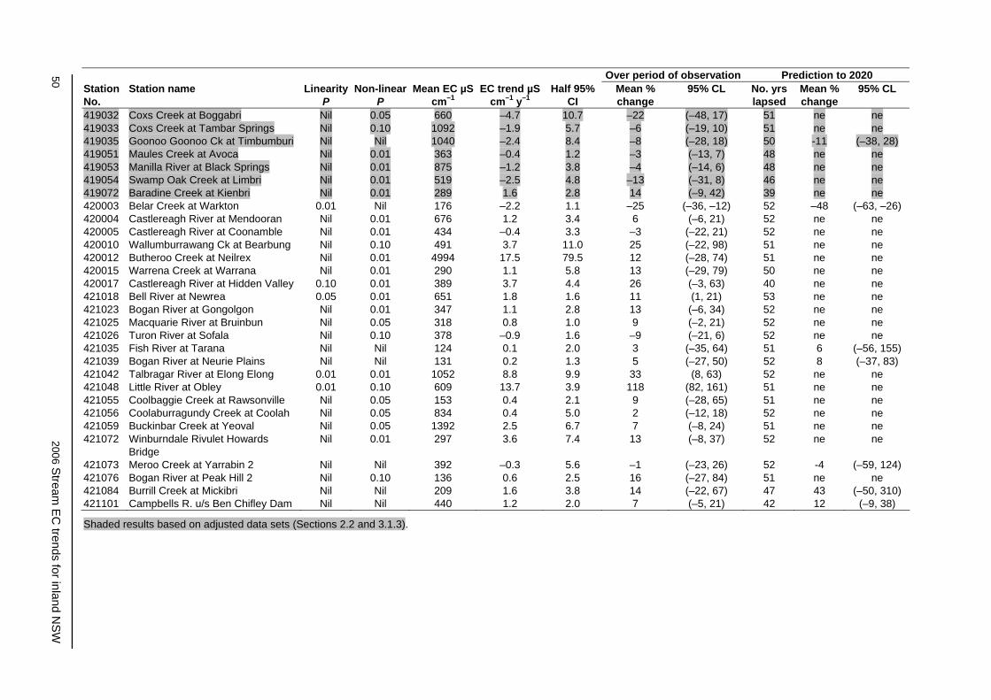
50 2006 S
tream E
C trends for inland N
SW
Over period of observation Prediction to 2020 Station No.
Station name Linearity P
Non-linear P
Mean EC µS cm–1
EC trend µS cm–1 y–1
Half 95% CI
Mean % change
95% CL No. yrs lapsed
Mean % change
95% CL
419032 Coxs Creek at Boggabri Nil 0.05 660 –4.7 10.7 –22 (–48, 17) 51 ne ne 419033 Coxs Creek at Tambar Springs Nil 0.10 1092 –1.9 5.7 –6 (–19, 10) 51 ne ne 419035 Goonoo Goonoo Ck at Timbumburi Nil Nil 1040 –2.4 8.4 –8 (–28, 18) 50 -11 (–38, 28) 419051 Maules Creek at Avoca Nil 0.01 363 –0.4 1.2 –3 (–13, 7) 48 ne ne 419053 Manilla River at Black Springs Nil 0.01 875 –1.2 3.8 –4 (–14, 6) 48 ne ne 419054 Swamp Oak Creek at Limbri Nil 0.01 519 –2.5 4.8 –13 (–31, 8) 46 ne ne 419072 Baradine Creek at Kienbri Nil 0.01 289 1.6 2.8 14 (–9, 42) 39 ne ne 420003 Belar Creek at Warkton 0.01 Nil 176 –2.2 1.1 –25 (–36, –12) 52 –48 (–63, –26) 420004 Castlereagh River at Mendooran Nil 0.01 676 1.2 3.4 6 (–6, 21) 52 ne ne 420005 Castlereagh River at Coonamble Nil 0.01 434 –0.4 3.3 –3 (–22, 21) 52 ne ne 420010 Wallumburrawang Ck at Bearbung Nil 0.10 491 3.7 11.0 25 (–22, 98) 51 ne ne 420012 Butheroo Creek at Neilrex Nil 0.01 4994 17.5 79.5 12 (–28, 74) 51 ne ne 420015 Warrena Creek at Warrana Nil 0.01 290 1.1 5.8 13 (–29, 79) 50 ne ne 420017 Castlereagh River at Hidden Valley 0.10 0.01 389 3.7 4.4 26 (–3, 63) 40 ne ne 421018 Bell River at Newrea 0.05 0.01 651 1.8 1.6 11 (1, 21) 53 ne ne 421023 Bogan River at Gongolgon Nil 0.01 347 1.1 2.8 13 (–6, 34) 52 ne ne 421025 Macquarie River at Bruinbun Nil 0.05 318 0.8 1.0 9 (–2, 21) 52 ne ne 421026 Turon River at Sofala Nil 0.10 378 –0.9 1.6 –9 (–21, 6) 52 ne ne 421035 Fish River at Tarana Nil Nil 124 0.1 2.0 3 (–35, 64) 51 6 (–56, 155) 421039 Bogan River at Neurie Plains Nil Nil 131 0.2 1.3 5 (–27, 50) 52 8 (–37, 83) 421042 Talbragar River at Elong Elong 0.01 0.01 1052 8.8 9.9 33 (8, 63) 52 ne ne 421048 Little River at Obley 0.01 0.10 609 13.7 3.9 118 (82, 161) 51 ne ne 421055 Coolbaggie Creek at Rawsonville Nil 0.05 153 0.4 2.1 9 (–28, 65) 51 ne ne 421056 Coolaburragundy Creek at Coolah Nil 0.05 834 0.4 5.0 2 (–12, 18) 52 ne ne 421059 Buckinbar Creek at Yeoval Nil 0.05 1392 2.5 6.7 7 (–8, 24) 51 ne ne 421072 Winburndale Rivulet Howards
Bridge Nil 0.01 297 3.6 7.4 13 (–8, 37) 52 ne ne
421073 Meroo Creek at Yarrabin 2 Nil Nil 392 –0.3 5.6 –1 (–23, 26) 52 -4 (–59, 124) 421076 Bogan River at Peak Hill 2 Nil 0.10 136 0.6 2.5 16 (–27, 84) 51 ne ne 421084 Burrill Creek at Mickibri Nil Nil 209 1.6 3.8 14 (–22, 67) 47 43 (–50, 310) 421101 Campbells R. u/s Ben Chifley Dam Nil Nil 440 1.2 2.0 7 (–5, 21) 42 12 (–9, 38)
Shaded results based on adjusted data sets (Sections 2.2 and 3.1.3).

Stream EC trends for inland NSW 2006 51
5.3 Catchment characteristics
The integration of catchment characteristics (Section 2.7) into the investigation increases the opportunity to explain EC trend behaviour in each catchment. The values are presented in Table 5, although some are not available for the more westerly catchments. It might be expected that some of the characteristics listed in Section 2.7 are interdependent. A matrix plot was produced for the catchment characteristics (Figure 26). It became necessary to remove the area of 5 sites, but only on the basis that they were greater than 8000 km2, preventing a clearer view of the effect of area in the plot. Similarly, very large mean ECs were removed at 420012 Butheroo Creek at Neilrex and 410103 Houlaghans Creek at Downside.
We hoped to use the characteristics to assist in arranging the sites into geographic groups on the basis that each group might exhibit common EC trend behaviour. We had to take care that the gauging station location was representative of the characteristics of its catchment; otherwise the process could have become confusing. The following sections describe how the groups were determined. The station details are described in Section 6.
5.3.1 Snowy subgroup
Figure 26 shows no pattern, except in mean annual rainfall versus elevation in Column 3. The plot emphasises a small group of stations that varied from the general pattern. Although these had high mean annual rainfall, their outlets had low elevation. These sites have been identified in Figure 27. Eight sites definitely varied from the majority pattern.
Two sites (labelled in blue in Figure 27) could have been included in the Snowy group but were not. One of these is 410024 Goodradigbee at Wee Jasper, which was attached to an adjoining subgroup with similar traits. The other was 410047 Tarcutta at Old Borambola, whose area (1640 km2) is nearly 3 times the size of the other 7 catchments. It has 2 distinct geographic components. Its top quarter is located in a mountainous, high-rainfall area—similar to the terrain of the other 7 sites—but its remainder is located in much flatter terrain with substantially less rainfall. Because of this variation in catchment characteristics, we decided not to categorise it in the Snowy subgroup.
Mathematically, there is no justification for the separation, because potentially there are an infinite number of locations that might fall in the area of interest outlined in Figure 27. In practice, there would be very few catchment sites in NSW that would be small enough to have such a high mean average rainfall and a low elevation. Six of the 7 sites became the basis of the Snowy subgroup.
5.3.2 Warrumbungle subgroup
The Warrumbungle Range protrudes onto the north-western plains of NSW, and defines the catchment boundary between the upper Castlereagh and the mid Namoi valleys. The terrain is unusual, with volcanic outcrops rising steeply out of the flat surrounding plains. There is a steep rainfall gradient on the range itself.
In their hypsometric work on the nearby Mooki River, Dowling et al. (1998) wrote ‘the catchment proved to be anomalous, and this was attributed to its size and internal complexity. … The outlier (Mooki) was later shown to have different land use patterns and considerable internal heterogeneity with respect to many soil/landscape variables’.
Mindful of Dowling et al.’s concerns, we grouped 4 sites on the basis that the Warrumbungle Range represented a large proportion of their area and gave a distorted value for the average slope of the catchment.
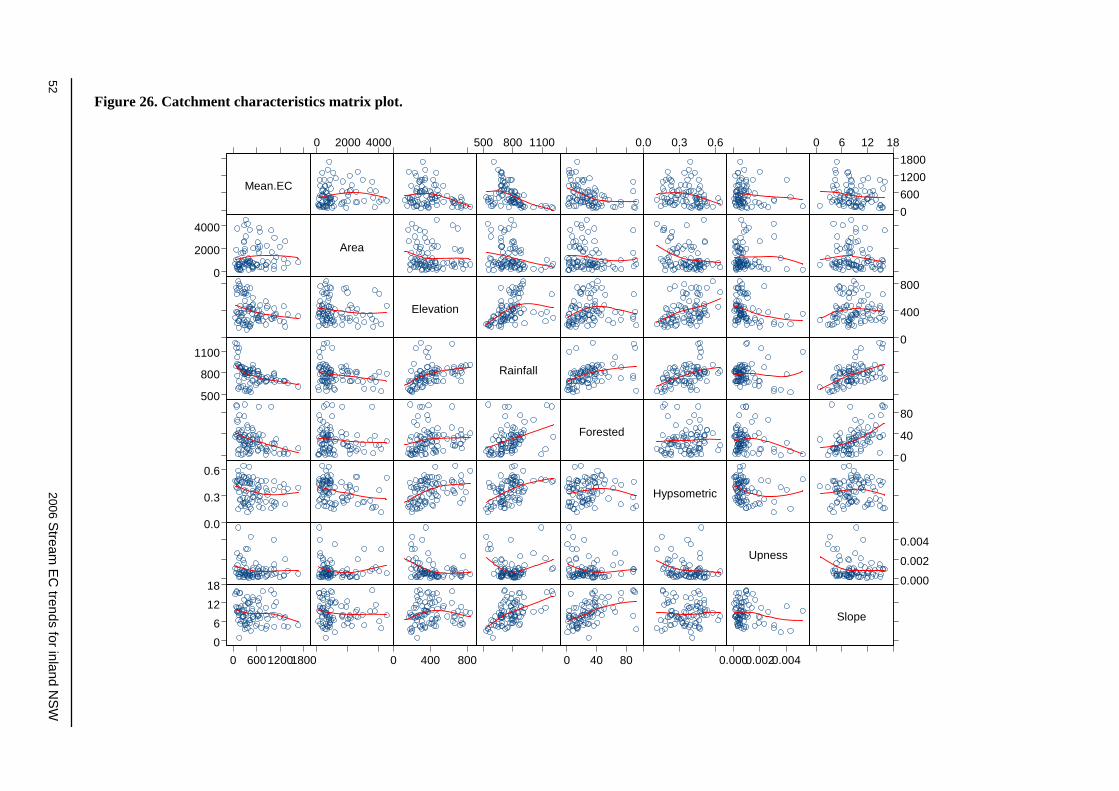
52 2006 S
tream E
C trends for inland N
SW
Figure 26. Catchment characteristics matrix plot.
Mean.EC
0
2000
4000
500
800
1100
0.0
0.3
0.6
06
1218
0 60012001800
0 2000 4000
Area
Elevation
0 400 800
500 800 1100
Rainfall
Forested
0 40 80
0.0 0.3 0.6
Hypsometric
Upness
0.0000.0020.004
060012001800
0 6 12 18
0
400
800
0
40
80
0.000
0.002
0.004
Slope
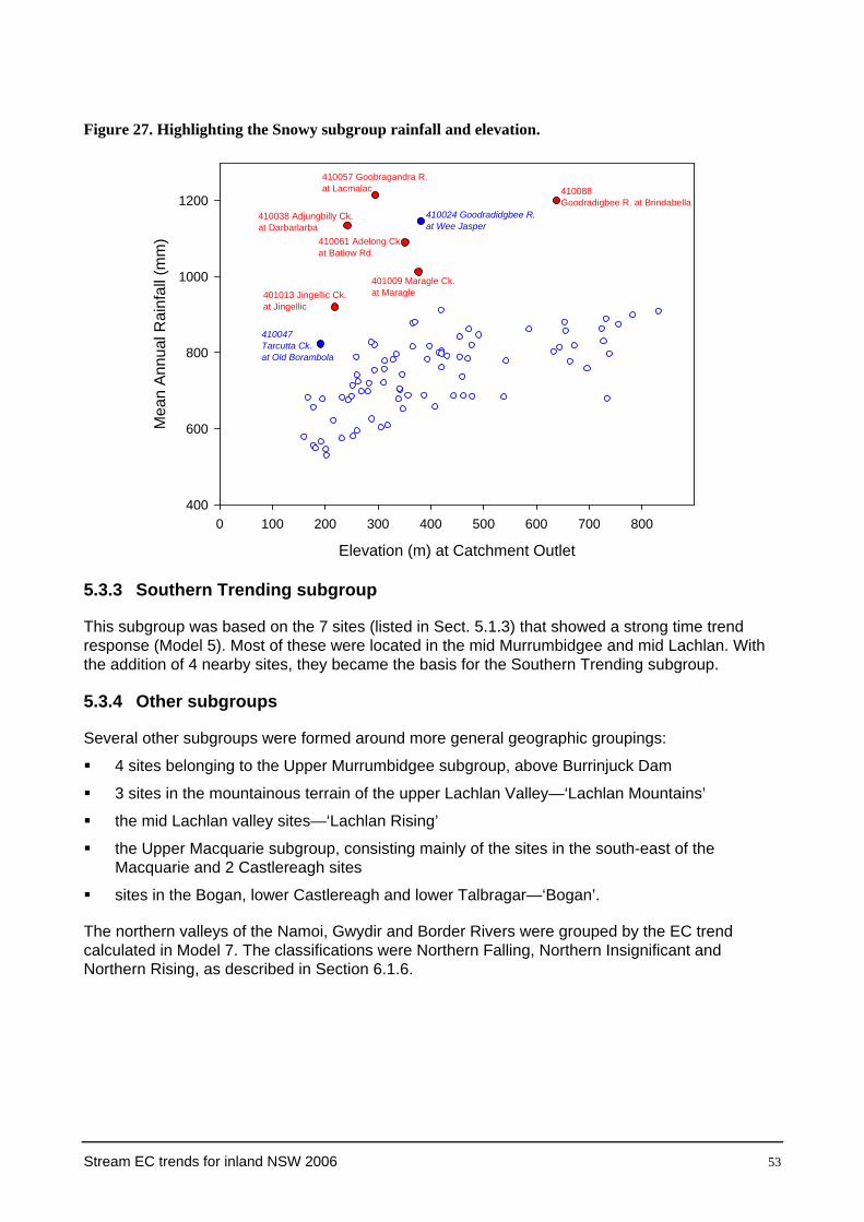
Stream EC trends for inland NSW 2006 53
The northern valleys of the Namoi, Gwydir and Border Rivers were grouped by the EC trend calculated in Model 7. The classifications were Northern Falling, Northern Insignificant and Northern Rising, as described in Section 6.1.6.
sites in the Bogan, lower Castlereagh and lower Talbragar—‘Bogan’.
the Upper Macquarie subgroup, consisting mainly of the sites in the south-east of the Macquarie and 2 Castlereagh sites
the mid Lachlan valley sites—‘Lachlan Rising’
3 sites in the mountainous terrain of the upper Lachlan Valley—‘Lachlan Mountains’
4 sites belonging to the Upper Murrumbidgee subgroup, above Burrinjuck Dam
Several other subgroups were formed around more general geographic groupings:
5.3.4 Other subgroups
This subgroup was based on the 7 sites (listed in Sect. 5.1.3) that showed a strong time trend response (Model 5). Most of these were located in the mid Murrumbidgee and mid Lachlan. With the addition of 4 nearby sites, they became the basis for the Southern Trending subgroup.
5.3.3 Southern Trending subgroup
Figure 27. Highlighting the Snowy subgroup rainfall and elevation.
Mea
n A
nnua
l Rai
nfal
l (m
m)
400
600
800
1000
1200
Elevation (m) at Catchment Outlet
0 100 200 300 400 500 600 700 800
410024 Goodradidgbee R.at Wee Jasper
410047Tarcutta Ck.at Old Borambola
410057 Goobragandra R.at Lacmalac
410038 Adjungbilly Ck.at Darbarlarba
410061 Adelong Ck.at Batlow Rd.
401009 Maragle Ck.at Maragle401013 Jingellic Ck.
at Jingellic
410088Goodradigbee R. at Brindabella

54 2006 S
tream E
C trends for inland N
SW
Table 5. Trend, cyclicity and catchment characteristics.
No. Station Name Mea
n a
nnua
l ra
infa
ll (
mm
)
Elev
atio
n a
t ga
uge
(m)
Ave
rage
sl
ope
catc
hmen
t
Line
ar
coef
ficie
nt
SE o
f lin
ear
coef
ficie
nt
P(s
lope
) = 0
(s
tat.
sign
if.)
Cyc
le ra
tio
% o
f cyc
le
Rec
over
y fa
ctor
Mea
n EC
Are
a (k
m2 )
UPN
ESS
mid
poin
t
Hyp
som
etric
in
tegr
al
% F
ores
ted
Mod
el 3
R2
Mod
el 5
R2 #
Mod
el 7
R2 ♫
Flow
%ile
H
ighe
st F
low
Snowy Sub-group401009 Maragle Ck. at Maragle 1012 376.6 9.1 0.0007 0.0019 Nil 1.08 37.0 0.96 108 216 0.00264 0.470 65.5 0.45 0.21 0.56 12401013 Jingellic Ck. at Jingellic 920 218.5 10.4 -0.0007 0.0009 Nil 1.03 12.9 0.98 114 394 0.00139 0.385 62.6 0.59 0.14 0.65 8410038 Adjungbilly Ck. at Darbalara 1135 241.8 10.5 -0.0015 0.0026 Nil 1.04 21.3 1.11 160 386 0.00212 0.475 17.0 0.46 0.04 0.49 4410057 Goobarragandra R. at Lacmalac 1214 295.2 14.8 0.0015 0.0020 Nil 1.04 16.7 1.00 59 665 0.00106 0.469 2.4 0.22 0.04 0.25 9410061 Adelong Ck. at Batlow Rd. 1090 351.5 9.4 -0.0008 0.0015 Nil 1.03 16.3 1.10 125 146 0.00526 0.484 36.6 0.46 0.05 0.49 25410088 Goodradigbee R. at Brindabella 1200 638.0 15.6 0.0007 0.0018 Nil 1.04 17.6 1.00 100 431 0.00097 0.458 3.2 0.66 0.10 0.69 2
Upper Murrumbidgee 410024 GoodradidgbeeR.at Wee Jasper 1146 381.0 15.4 -0.0043 0.0013 0.01 1.06 25.8 1.12 86 990 * * 11.9 0.63 0.20 0.71 16410033 Murrumbidgee R.at Mittagang Xing 889 732.0 10.8 -0.0100 0.0025 0.01 1.10 37.8 1.79 76 1891 0.00063 0.401 3.8 0.08 0.14 0.22 *410050 Murrumbidgee R. at Billilingra 759 696.0 9.3 -0.0087 0.0019 0.01 1.08 35.1 1.29 100 3745 * * 34.6 0.09 0.18 0.27 19410062 Numeralla R. at Numeralla Sch. 680 734.0 8.1 -0.0074 0.0017 0.01 1.07 34.2 1.24 144 675 0.00020 0.528 34.8 0.56 0.16 0.63 38410107 Mountain Ck. at Mountain Ck. 877 366.0 15.2 0.0101 0.0026 0.01 1.09 43.6 0.70 164 167 0.00046 0.424 73.5 0.69 0.13 0.73 32420003 Belar Ck. at Warkton 863 472.3 15.0 -0.0124 0.0034 0.01 1.04 21.2 1.16 176 131 0.00020 0.252 33.9 0.21 0.07 0.27 5
Southern Trending Sub-group410025 Jugiong Ck. at Jugiong 685 249.3 7.7 0.0195 0.0016 0.01 1.08 55.0 0.57 1184 2140 0.00015 0.399 20.9 0.52 0.42 0.74 5410044 Muttama Ck. at Coolac 683 232.3 7.3 0.0112 0.0023 0.01 1.06 42.0 0.90 1294 1059 0.00035 0.343 39.7 0.59 0.18 0.68 14410045 Billabung Ck. at Sunnyside 622 215.2 7.7 0.0269 0.0133 0.10 1.09 46.3 0.62 257 842 0.00193 0.219 12.5 0.13 0.12 0.29 20410047 Tarcutta Ck. at Old Borambola 823 190.7 7.6 0.0127 0.0013 0.01 1.08 41.3 0.79 254 1641 0.00016 0.277 3.6 0.42 0.39 0.65 1410048 Kyeamba Ck. at Ladysmith 678 195.2 8.3 0.0213 0.0027 0.01 1.12 70.5 0.55 836 550 0.00102 0.233 3.5 0.54 0.31 0.70 1410091 Billabong Ck. at Walbundrie 683 167.1 7.4 0.0195 0.0026 0.01 1.11 65.5 0.52 1324 2657 0.00200 0.204 47.1 0.73 0.27 0.81 37410097 Billabong Ck. at Aberfeldy 698 268.4 7.4 0.0109 0.0019 0.01 1.06 37.4 0.72 507 346 0.00037 0.290 90.1 0.55 0.18 0.63 23410103 Houlaghans Ck. at Downside 567 191.6 2.7 0.1852 0.0115 0.01 1.90 195.0 0.01 4707 1144 0.00357 0.396 0.9 0.59 0.37 0.95 0412099 Manna Ck. near Lake Cowal 531 202.4 3.1 0.0223 0.0069 0.01 1.12 64.5 0.67 451 10857 0.00432 0.154 8.4 0.29 0.38 0.57 15412103 Bland Ck. at Morangarell 576 230.7 4.9 0.0871 0.0176 0.01 1.23 106.0 0.35 326 3050 0.00307 0.232 7.6 0.26 0.46 0.61 23
Lachlan Mountains Sub-group412028 Abercrombie R. at Abercrombie 805 420.0 9.8 -0.0023 0.0017 Nil 1.01 4.0 1.08 280 2625 0.00014 0.512 37.2 0.58 0.01 0.58 14412050 Crookwell R. at Narrawa North 789 454.8 6.5 -0.0008 0.0021 Nil 1.01 5.5 1.11 418 756 0.00047 0.625 10.6 0.66 0.00 0.65 12412083 Tuena Ck. at Tuena 820 477.4 10.0 -0.0100 0.0027 Nil 1.01 9.1 1.03 483 320 0.00019 0.437 50.3 0.68 0.01 0.69 20
Lachlan Rising Sub-group410026 Yass R. at Yass 685 478.0 7.1 0.0080 0.0036 0.05 1.04 25.6 0.83 688 2171 0.00029 0.295 92.0 0.36 0.03 0.37 2412009 Belubula R. at Canowindra 821 292.8 8.1 0.0045 0.0018 0.05 1.02 13.5 0.86 643 2133 0.00023 0.418 9.9 0.48 0.08 0.52 15412030 Mandagery Ck. at U/S Eugowra 698 280.4 8.3 0.0138 0.0032 0.01 1.04 30.1 0.61 987 1689 0.00043 0.239 22.1 0.42 0.23 0.57 40412043 Goobang Ck. at Darbys Dam 547 201.3 4.0 0.0284 0.0092 0.01 1.04 21.9 0.69 364 4172 0.00304 0.113 13.2 0.43 0.14 0.51 *412055 Belubula R. at Bangaroo Bridge 789 259.2 7.8 0.0056 0.0040 Nil 1.03 18.1 0.76 624 2550 0.00018 0.379 8.9 0.40 0.12 0.48 *412065 Lachlan R. at Narrawa 688 443.1 4.8 0.0044 0.0022 0.05 1.03 17.3 0.87 855 2252 0.00033 0.350 11.8 0.56 0.06 0.59 8412072 Back Ck. at Koorawatha 609 318.4 4.8 0.0162 0.0079 0.05 1.02 15.9 0.74 1665 800 0.00050 0.393 14.0 0.38 0.05 0.41 11412086 Goobang Ck. at Parkes 626 287.4 4.7 -0.0146 0.0064 0.05 1.06 32.7 1.15 573 653 0.00162 0.338 36.4 0.60 0.08 0.63 19412096 Pudmans Ck. at Kennys Rd 687 461.8 4.6 0.0028 0.0038 Nil 1.02 10.8 0.84 1294 331 0.00033 0.429 6.5 0.71 0.00 0.71 6

Table 5. Trend, cyclicity and catchment characteristics (continued) 2006 Stream
EC
trends for inland NSW
55
No. Station Name Mea
n a
nnua
l ra
infa
ll (
mm
)
Elev
atio
n a
t ga
uge
(m)
Ave
rage
sl
ope
catc
hmen
t
Line
ar
coef
ficie
nt
SE o
f lin
ear
coef
ficie
nt
P(s
lope
) = 0
(s
tat.
sign
if.)
Cyc
le ra
tio
% o
f cyc
le
Rec
over
y fa
ctor
Mea
n EC
Are
a (k
m2 )
UPN
ESS
mid
poin
t
Hyp
som
etric
in
tegr
al
% F
ores
ted
Mod
el 3
R2
Mod
el 5
R2
#
Mod
el 7
R2 ♫
Flow
%ile
hi
ghes
t flo
w
Upper Macquarie Sub-group 420004 Castlereagh R. at Mendooran 706 340.6 9.3 0.0018 0.0019 Nil 1.03 16.7 0.83 676 3451 0.00078 0.241 28.7 0.59 0.10 0.63 17421025 Macquarie R. at Bruinbun 785 470.2 8.1 0.0024 0.0015 Nil 1.03 15.5 0.90 318 4507 0.00059 0.504 26.5 0.53 0.03 0.55 22421026 Turon R. at Sofala 803 632.7 12.1 -0.0025 0.0021 Nil 1.03 19.1 0.94 378 880 0.00024 0.474 51.6 0.66 0.03 0.67 6421035 Fish R. at Tarana 909 831.0 8.8 0.0012 0.0087 Nil 1.05 21.9 0.88 124 593 0.00047 0.579 41.3 0.21 0.00 0.21 21421056 Coolaburragundy Ck. at Coolah 684 538.4 10.5 0.0005 0.0025 Nil 1.01 8.7 0.95 834 212 0.00024 0.384 9.1 0.32 0.04 0.34 39421072 Winburndale Rivlt at Howards Bdge 778 542.6 11.1 0.0119 0.0101 Nil 1.04 23.0 * 297 720 0.00041 0.446 38.1 0.67 0.20 0.73 2421073 Meroo Ck. at Yarrabin 2 818 397.5 11.8 -0.0008 0.0083 Nil 1.00 1.9 1.02 392 729 0.00006 0.505 35.2 0.59 0.00 0.57 *421101 Campbells R. U/S Ben Chifley Dam 830 727.1 6.5 0.0027 0.0025 Nil 1.01 8.3 0.94 440 918 0.00032 0.465 22.1 0.78 0.00 0.78 21
Central Macquarie Sub-group420012 Butheroo Ck. at Neilrex 688 387.1 5.6 0.0035 0.0070 Nil 1.08 62.5 0.85 4994 405 0.00191 0.325 41.3 0.79 0.15 0.82 67421018 Bell R. at Newrea 757 311.7 7.9 0.0027 0.0012 0.05 1.01 9.2 0.92 651 1629 0.00075 0.282 89.6 0.65 0.09 0.68 15421042 Talbragar R. at Elong Elong 679 339.1 8.2 0.0083 0.0031 0.01 1.08 51.0 0.73 1052 2963 0.00054 0.226 20.6 0.34 0.12 0.42 16421048 Little R. at Obley 658 407.8 5.4 0.0223 0.0026 0.01 1.12 66.3 0.50 609 577 0.00026 0.358 28.2 0.65 0.30 0.76 99421059 Buckinbar Ck. at Yeoval 653 346.5 4.5 0.0018 0.0022 Nil 1.04 27.0 0.90 1392 701 0.00082 0.380 3.7 0.53 0.07 0.56 3
Bogan Sub-group420005 Castlereagh R. at Coonamble 657 176.9 8.8 -0.0009 0.0034 Nil 1.04 26.2 0.92 434 8302 * 0.268 27.9 0.74 0.18 0.79 0420015 Warrena Ck. at Warrana 550 181.1 3.7 0.0039 0.0076 Nil 1.19 87.3 0.57 290 621 * 0.181 93.7 0.38 0.14 0.47 30421023 Bogan R. at Gongolgon * 122.5 * 0.0033 0.0025 Nil 1.05 30.7 0.82 347 27970 * * 0.32 0.11 0.39 63421039 Bogan R. at Neurie Plains * * * 0.0014 0.0052 Nil 1.04 19.8 1.01 131 14760 * * 0.09 0.00 0.05 74421055 Coolbaggie Ck. at Rawsonville 596 260.3 0.9 0.0025 0.0060 Nil 1.13 56.7 1.05 153 566 * 0.408 29.6 0.10 0.07 0.16 4421076 Bogan R. at Peak Hill 2 581 252.3 6.4 0.0045 0.0071 Nil 1.06 28.2 0.84 136 1099 * 0.146 9.9 0.14 0.11 0.23 31421084 Burrill Ck. at Mickibri 603 306.0 6.2 0.0076 0.0114 Nil 1.08 39.4 * 209 71 * 0.182 2.2 0.32 0.01 0.34 51
Warrumbungle Sub-group419027 Mooki R. at Breeza 721 282.6 16.0 0.0127 0.0023 0.01 1.08 52.7 0.70 975 3587 0.00098 0.160 89.5 0.23 0.24 0.42 14419072 Baradine Ck. at Kienbri 725 261.9 13.0 0.0056 0.0049 Nil 1.06 33.5 0.78 289 982 0.00165 0.205 72.5 0.60 0.20 0.70 35420010 Wallumburrawang Ck. at Bearbung 688 356.7 9.4 0.0076 0.0081 Nil 1.04 26.0 0.80 491 434 0.00057 0.231 21.7 0.36 0.07 0.41 28420017 Castlereagh R. at Hidden Valley 762 420.3 11.9 0.0095 0.0055 0.10 1.06 37.1 * 389 1147 0.00058 0.201 26.6 0.31 0.11 0.38 43
Norther Falling Sub-group416008 Beardy R. at Haystack 796 334.7 9.6 -0.0098 0.0021 0.01 1.09 32.3 1.13 233 903 0.00057 0.534 46.4 0.37 0.22 0.51 33418005 Copes Ck. at Kimberley 875 756.0 5.3 -0.0066 0.0021 0.01 1.03 15.2 1.17 178 235 0.00232 0.262 29.8 0.51 0.05 0.54 38418014 Gwydir R. at Yarrowyck 798 738.4 5.5 -0.0044 0.0017 0.01 1.02 12.0 1.12 357 827 0.00035 0.441 14.0 0.63 0.03 0.65 30418025 Halls Ck. at Bingara 779 313.0 11.0 -0.0045 0.0013 0.01 1.02 16.9 1.10 1039 171 0.00402 0.368 23.6 0.02 0.12 0.14 44418027 Horton R. at DamSite 912 419.6 13.8 -0.0183 0.0030 0.01 1.10 53.7 1.69 506 207 0.00087 0.355 46.9 0.64 0.22 0.72 22419005 Namoi R. at North Cuerindi 816 365.5 9.2 -0.0116 0.0038 0.01 1.07 33.1 1.44 278 2524 0.00070 0.512 23.9 0.55 0.08 0.59 22419016 Cockburn R. at Mulla Crossing 841 454.3 12.2 -0.0100 0.0021 0.01 1.03 16.8 1.34 434 893 0.00080 0.444 37.6 0.27 0.11 0.36 28419029 Halls Ck. at Ukalon 783 393.4 13.4 -0.0065 0.0025 0.05 1.04 25.5 1.08 669 357 0.00053 0.394 39.5 0.58 0.14 0.64 25
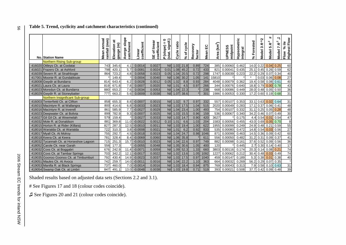
56 2006 S
tream E
C trends for inland N
SW
Table 5. Trend, cyclicity and catchment characteristics (continued)
No. Station Name Mea
n an
nual
ra
infa
ll (m
m)
Elev
atio
n at
ga
uge
(m)
Ave
rge
slop
e ca
tchm
ent
Line
ar
coef
ficie
nt
SE o
f lin
ear
coef
ficie
nt
P(s
lope
) = 0
(s
tat.
sign
if.)
Cyc
le ra
tio
% o
f cyc
le
Rec
over
y fa
ctor
Mea
n EC
Are
a (k
m2 )
UPN
ESS
mid
poin
t
Hyp
som
etric
in
tegr
al
% F
ores
ted
Mod
el 3
R^2
Mod
el 5
R2
#
Mod
el 7
R2
♫Fl
ow %
ile
Hig
hest
Flo
w
Northern Rising Sub-group416020 Ottleys Ck. at Coolatai 743 345.6 4.1 0.0014 0.0027 Nil 1.03 21.8 0.89 724 385 0.00060 0.462 14.0 0.22 0.04 0.25 60416021 Frazers Ck. at Ashford 798 420.1 5.7 0.0081 0.0024 0.01 1.08 45.2 0.72 433 821 0.00041 0.435 25.1 0.45 0.26 0.59 62416039 Severn R. at Strathbogie 864 723.2 4.8 0.0058 0.0023 0.05 1.04 20.5 0.72 298 1747 0.00039 0.223 22.2 0.29 0.07 0.34 40417001 Moonie R. at Gundablouie * 149.4 * 0.0004 0.0040 Nil 1.06 30.2 1.05 141 15810 * * * 0.03 0.06 0.08 27418008 Gwydir at Bundarra 814 643.4 6.2 0.0028 0.0012 0.05 1.02 8.8 0.93 284 4048 0.00079 0.362 19.4 0.58 0.08 0.61 40418021 Laura Ck. at Laura 819 671.8 7.8 0.0007 0.0020 Nil 1.01 4.5 0.97 266 344 0.00076 0.640 18.8 0.79 0.00 0.78 43418023 Moredun Ck. at Bundarra 880 653.2 7.6 0.0034 0.0053 Nil 1.04 22.3 * 238 668 0.00086 0.449 28.0 0.48 0.05 0.50 36418029 Gwydir R. at Stoneybatter 777 663.2 5.6 0.0009 0.0038 Nil 1.07 38.6 * 301 1986 0.00053 0.330 17.2 0.60 0.19 0.68 31
Northern Insignificant Sub-group416003 Tenterfield Ck. at Clifton 858 655.3 8.8 -0.0007 0.0015 Nil 1.02 9.7 0.97 332 557 0.00107 0.353 33.1 0.63 0.02 0.64 31416010 Macintyre R. at Wallangra 800 414.6 6.8 -0.0033 0.0023 Nil 1.03 17.5 1.04 515 2020 0.00049 0.283 17.1 0.37 0.06 0.41 48416016 Macintyre R. at Inverell 861 585.9 7.7 -0.0027 0.0029 Nil 1.04 23.4 1.00 493 754 0.00107 0.332 31.1 0.25 0.05 0.28 48416023 Deepwater Ck. at Bolivia 899 782.9 9.3 -0.0007 0.0025 Nil 1.03 15.5 0.96 159 536 0.00067 0.340 34.2 0.46 0.07 0.49 30416027 Gil Gil Ck. at Weemelah 579 159.4 * 0.0027 0.0033 Nil 1.03 14.7 0.90 420 3627 * 0.175 4.4 0.54 0.01 0.54 47416032 Mole R. at Donaldson 881 369.8 11.0 -0.0022 0.0012 0.10 1.01 6.6 1.03 204 1583 0.00056 0.455 43.0 0.69 0.05 0.70 8418015 Horton R. at Rider (Killara) 827 287.3 12.5 -0.0010 0.0011 Nil 1.03 19.4 1.00 622 1955 0.00099 0.249 24.9 0.48 0.21 0.59 55418016 Warialda Ck. at Warialda 722 310.3 3.8 -0.0008 0.0021 Nil 1.01 6.2 0.92 833 535 0.00080 0.472 14.8 0.54 0.03 0.56 27418017 Myall Ck. At Molroy 755 292.7 4.5 -0.0018 0.0019 Nil 1.04 24.7 0.98 1046 871 0.00099 0.463 14.5 0.36 0.09 0.42 60418018 Keera Ck. at Keera 781 328.4 8.4 -0.0069 0.0060 Nil 1.06 35.8 * 611 556 0.00050 0.482 31.2 0.31 0.09 0.37 41418032 Tycannah Ck. at Horseshoe Lagoon 715 251.3 15.7 -0.0010 0.0023 Nil 1.04 22.6 0.97 749 882 0.00098 0.161 37.6 0.52 0.09 0.56 36418052 Carole Ck. near Garah 556 177.3 * -0.0055 0.0048 Nil 1.05 30.6 1.05 400 120 * 0.445 2.7 0.30 0.14 0.40 17419032 Coxs Ck. at Boggabri 676 242.9 11.4 -0.0071 0.0059 Nil 1.09 52.3 1.33 660 3803 0.00116 0.174 20.3 0.14 0.08 0.21 74419033 Coxs Ck. at Tambar Springs 703 342.2 12.1 -0.0017 0.0022 Nil 1.02 13.6 1.05 1092 1227 0.00062 0.212 30.4 0.48 0.03 0.49 74419035 Goonoo Goonoo Ck. at Timbumburi 792 430.4 14.9 -0.0023 0.0037 Nil 1.03 17.5 0.97 1040 459 0.00147 0.189 5.3 0.38 0.01 0.38 40419051 Maules Ck. At Avoca 742 259.7 14.0 -0.0011 0.0016 Nil 1.04 22.2 1.10 363 664 0.00032 0.269 56.2 0.29 0.07 0.35 *419053 Manilla R. at Black Springs 737 460.0 7.0 -0.0014 0.0016 Nil 1.03 18.4 0.94 875 769 0.00043 0.313 7.9 0.58 0.10 0.63 31419054 Swamp Oak Ck. at Limbri 847 491.1 13.0 -0.0048 0.0038 Nil 1.03 19.8 0.71 519 393 0.00021 0.508 37.7 0.42 0.09 0.48 39
Shaded results based on adjusted data sets (Sections 2.2 and 3.1).
# See Figures 17 and 18 (colour codes coincide).
♫ See Figures 20 and 21 (colour codes coincide).

Stream EC trends for inland NSW 2006 57
Apart from the elevation vs mean annual rainfall plot, little was obvious. Model 5 and elevation (row 2, column 5) suggested that the time trend had very little relevance to catchments with high-elevation outlets. But some catchments with low elevation (listed in Section 5.1.3) seemed to have a high degree of fit to Model 5. The catchments with the stronger trend components were nearly all in the southern valleys. Based on row 2 of Figure 29, their outlets had comparatively low elevation, their forested percentage was small, and their average slope was at the low end of the range.
We generated plots to examine the link between model performance and the physical characteristics in the field. In Figure 29, all the catchment characteristics are plotted for all sites, excluding the 6 sites of the Snowy subgroup. The plots are supplemented with a smoothing spline (3 df). The areas of 5 sites were removed on the basis that they were outliers preventing a clearer view of the effect of area in the matrix plot. Two sites were also removed owing to very high EC values: 420012 Butheroo Creek at Neilrex and 410103 Houlaghans Creek at Downside (EC = 4994 and 4707 µS cm–1 respectively).
5.4 Model performance and catchment characteristics
Figure 28. Mean EC envelope.
One of the minor traits in the catchment characteristics matrix plot (Figure 26) relates to the mean EC and mean annual rainfall (row 1, column 4). A mean EC envelope has been plotted as Figure 28. The plot does not represent a rigorous concept, because the sampling is infrequent. However, it is of interest because it demonstrates that highly saline catchments are unlikely to be found in high rainfall areas.
5.3.5 Mean EC envelope M
ean
EC
0
500
1000
1500
2000
2500
3000
HypsomePlot 1
tric vs Linear Upper specification
Mean annual rainfall (mm)
600 800 1000 1200

58 2006 S
tream E
C trends for inland N
SW
Figure 29. Model performance and catchment characteristics (excluding Snowy group).
Model.3
0.00.20.4
020004000
500800
1100
0.0
0.3
0.6
06
1218
0.0 0.3 0.6
0.0 0.2 0.4
Model.5
Model.7
0.0 0.4 0.8
0 20004000
Area
Elevation
0 400 800
500 8001100
Rainfall
Forested
0 40 80
0.0 0.3 0.6
Hypsometric
Upness
0.0000.0020.004
0 6 12 18
Slope
0.00.30.6
0.00.40.8
0
400
800
04080
0.0000.0020.004
MeanEC060012001800
0 60012001800

6 Preliminary Catchment Groups
Figure 30. Subgroups in southern NSW.
2006 Stream EC trends for inland NSW 59

6.1 Categorisation (southern valleys)
6.1.1 Southern catchments in equilibrium
Three of the subgroups of Section 5.3 and Figure 30 are strong candidates for the equilibrium category.
a) Snowy subgroup (6) 401009 Maragle Creek at Maragle
401013 Jingellic Creek at Jingellic
410038 Adjungbilly Creek at Darbalara
410057 Goobarragandra River at Lacmalac
410061 Adelong Creek at Batlow Road
410088 Goodradigbee River at Brindabella
We concluded that this subgroup was more or less in equilibrium, with none of the trend slopes being statistically significant. The cyclic indicators were small, but not negligible.
General characteristics:
All have a data gap in the early 1990s. We have assumed there are sufficient data-points after the gap.
The mean annual rainfalls are in the high range. The lowest is at Jingellic (920 mm), and the rest are >1000 mm.
Elevations are generally in the range of 218 to 377 m, except Goodradigbee at Brindabella at 638 m.
Low non-significant trend slopes are close to zero; largest loge slope is +0.0015 for 410057 for Goobarragandra River at Lacmalac. The slope is not significant.
The recovery range is 0.96 to 1.11.
The percentage of cycle ranges from 13% to 21%; However, 401009 Maragle at Maragle has 37%, suggesting catchment heterogeneity.
The cycle ratios were 1.03 to 1.04, except Maragle Creek again at 1.08.
Average catchment slopes are >9.
The graphs of the unadjusted data in Appendix 2 indicate that these sites have not (or only just) completed the cycle. A reliable assessment of trend can’t really be made until a full cycle is complete.
The sites were in the top half of the hypsometric rankings (5 of them in the top quarter).
Three of the catchments were heavily forested, 1 moderately so, and 2 low.
The trend at 401013 Jingellic Creek at Jingellic may be rising once more. In the 1980s and 1990s this site peaked much earlier than the other Murrumbidgee–Murray sites. It is possibly heralding a general trend upturn. Even if it is the only site rising, in about 10 years it may have achieved another peak, which will enable a comparison of successive EC peaks and thus provide a better insight into the long-term trends of this subgroup.
See Figure 31 for a GAM curve typical of this subgroup.
2006 Stream EC trends for inland NSW 60
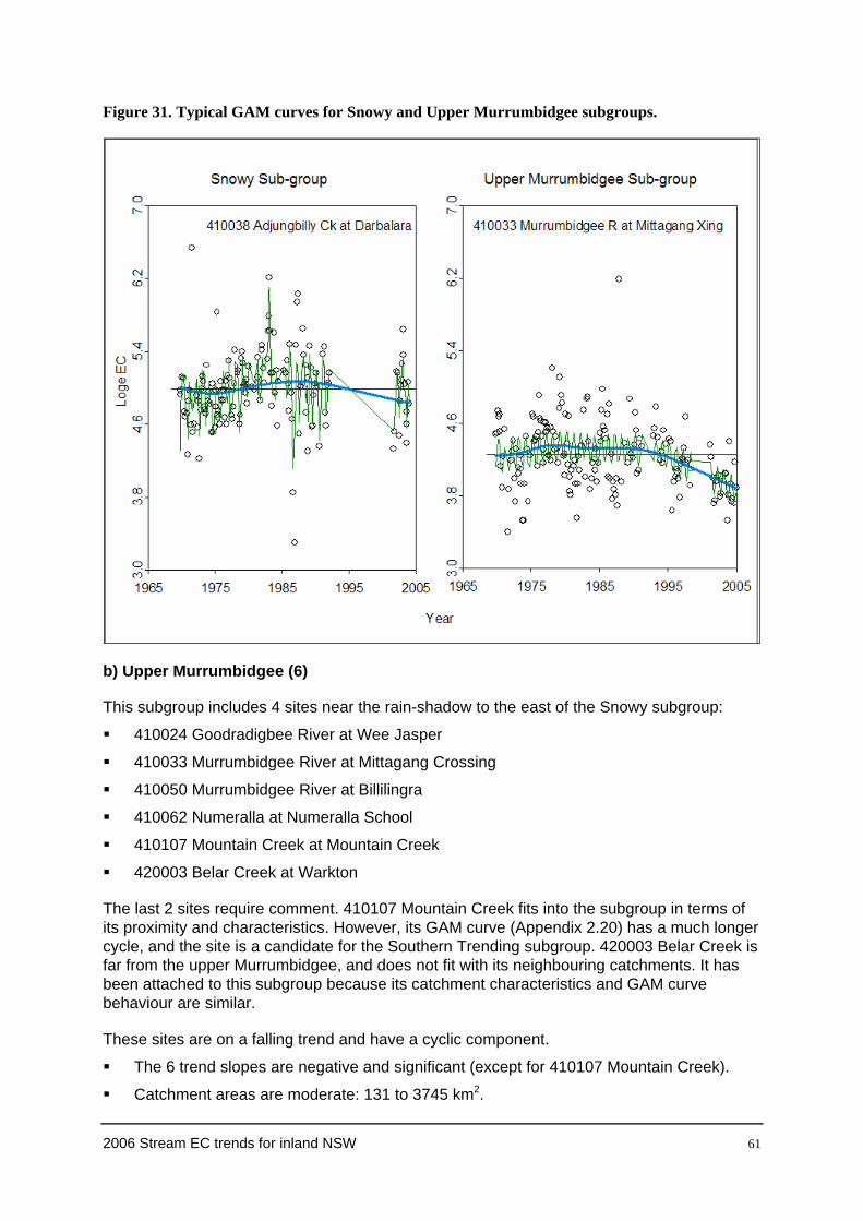
Figure 31. Typical GAM curves for Snowy and Upper Murrumbidgee subgroups.
b) Upper Murrumbidgee (6)
This subgroup includes 4 sites near the rain-shadow to the east of the Snowy subgroup:
410024 Goodradigbee River at Wee Jasper
410033 Murrumbidgee River at Mittagang Crossing
410050 Murrumbidgee River at Billilingra
410062 Numeralla at Numeralla School
410107 Mountain Creek at Mountain Creek
420003 Belar Creek at Warkton
The last 2 sites require comment. 410107 Mountain Creek fits into the subgroup in terms of its proximity and characteristics. However, its GAM curve (Appendix 2.20) has a much longer cycle, and the site is a candidate for the Southern Trending subgroup. 420003 Belar Creek is far from the upper Murrumbidgee, and does not fit with its neighbouring catchments. It has been attached to this subgroup because its catchment characteristics and GAM curve behaviour are similar.
These sites are on a falling trend and have a cyclic component.
The 6 trend slopes are negative and significant (except for 410107 Mountain Creek).
Catchment areas are moderate: 131 to 3745 km2.
2006 Stream EC trends for inland NSW 61

Mean annual rainfalls are within a narrow band of 680 to 889 mm except for 410024 at 1146 mm.
Outlet elevations range from 366 to 734 m.
Recovery ranges from 1.12 to 1.79.
The percentage of cycle range is 21% to 44%.
The cycle ratio is 1.04 to 1.10.
Average catchment slopes are 8.1 to 15.4.
Mean ECs are all <176 µS/cm.
See Figure 31 for a GAM curve typical of this subgroup.
c) Lachlan mountains subgroup (3) 412028 Abercrombie River at Abercrombie
412050 Crookwell River at Narrawa North
412083 Tuena Creek at Tuena
With only 5 data points after a gap in time, 412083 probably needs another 12 months of records before we can be definitive about its trend. The statistics are more appropriate to the period 1968–1992.
General characteristics:
The 3 trend slopes are small, negative and insignificant.
Mean annual rainfall varies from 789 to 820 mm.
Elevations are in the range of 420 to 480 m.
The low negative trend slope (not significant) is close to zero.
Resilience ranges from 1.03 to 1.11.
The cyclicity range is 4% to 9.1%.
Average catchment slopes are 6.45 (Narrawa North), 9.8 and 10.
See Figure 32 for a GAM curve typical of this subgroup.
6.1.2 Lachlan Rising subgroup (9) 410026 Yass River at Yass
412009 Belubula River at Canowindra
412030 Mandagery Creek upstream of Eugowra
412043 Goobang Creek at Darbys Dam
412055 Belubula River at Bangaroo Bridge
412065 Lachlan at Narrawa
412072 Back Creek at Koorawatha
412086 Goobang at Parkes
412096 Pudmans Creek at Kennys Road
2006 Stream EC trends for inland NSW 62

Two sites that would currently benefit from another year of monthly EC samples: 412096 and 412030. Unlike the Murrumbidgee–Murray sites, the Lachlan sites appear to be on a shorter cycle than the period of record. In assessing some of these sites, we have relied heavily on the plots in Appendices 2.21 to 2.33. Because of the data gaps and irregular periods of record, it is necessary to check how a short period of record at a particular site dovetails into the longer records at other sites. For example, the negative slope at 412086 coincides with a falling phase at other stations. The site has been included in this subgroup despite showing a recovery factor of >1 and a positive slope.
General characteristics:
Mean annual rainfall ranges from 546 to 820 mm.
Elevation ranges from 201 m (412043 Goobang at Darbys Dam) to 478 m.
The trend slopes are all positive (except at 412086), which is discussed above. They range from 0.0028 to 0.0284 (again, 412043), and 5 of these are significant. Hypothetically, if the 15% correction were applied as suggested in Annexure A, then the slope at 4 of the 8 sites would be statistically insignificant. But such a correction will not change the overall positive trend of the subgroup.
Resilience of the 7 sites with a positive log slope ranges from 0.61 to 0.87.
Cyclicity ranges from 11% to 33%.
Average catchment slopes range from 4.0 (412043) to 8.3.
The cycle ratio varies from 1.02 to 1.06 (412086).
Several of these catchments show little response to Model 5, indicating no or small trends over time.
See Figure 32 for a GAM curve typical of this subgroup.
412043 Goobang at Darbys Dam has sufficient extreme characteristics to make it a candidate for Southern Trending (Section 6.1.3). Both of the Belubula River catchments (412009 and 412055) border on characteristics that would place them in the Lachlan Mountains subgroup in Equilibrium (Section 6.1.1). Indeed, had the 412009 Belubula at Canowindra gauging site been located further up the catchment, its catchment characteristics would have assigned it to the Lachlan Mountains subgroup.
2006 Stream EC trends for inland NSW 63
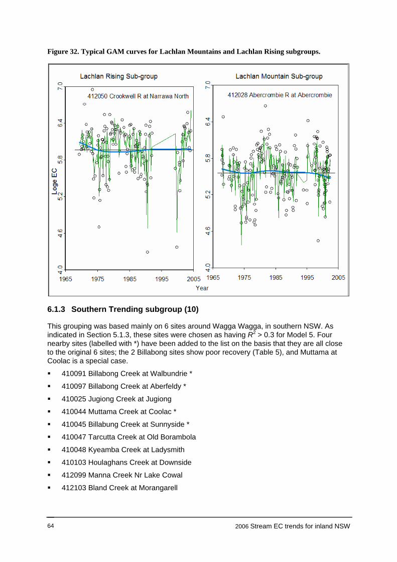
Figure 32. Typical GAM curves for Lachlan Mountains and Lachlan Rising subgroups.
6.1.3 Southern Trending subgroup (10)
This grouping was based mainly on 6 sites around Wagga Wagga, in southern NSW. As indicated in Section 5.1.3, these sites were chosen as having R2 > 0.3 for Model 5. Four nearby sites (labelled with *) have been added to the list on the basis that they are all close to the original 6 sites; the 2 Billabong sites show poor recovery (Table 5), and Muttama at Coolac is a special case.
410091 Billabong Creek at Walbundrie *
410097 Billabong Creek at Aberfeldy *
410025 Jugiong Creek at Jugiong
410044 Muttama Creek at Coolac *
410045 Billabung Creek at Sunnyside *
410047 Tarcutta Creek at Old Borambola
410048 Kyeamba Creek at Ladysmith
410103 Houlaghans Creek at Downside
412099 Manna Creek Nr Lake Cowal
412103 Bland Creek at Morangarell
2006 Stream EC trends for inland NSW 64

Figure 33. Typical GAM curves for Southern Trending subgroup.
Three other sites scattered across the area could have easily been categorised in the Southern Trending subgroup because of their GAM curve behaviour. Instead, they have been placed in local subgroups. These are:
410107 Mountain Creek at Mountain Creek
419027 Mooki River at Breeza (the behaviour of both sites is discussed in Section 7)
421048 Little River at Obley
General characteristics:
The range of mean annual rainfall is 531 to 698 mm, except 410047 Tarcutta Old Borambola is at 823 mm. Originally (Section 5.3.1), this was considered for inclusion in the nearby Snowy subgroup on the basis of its rainfall average. However, most of the catchment has characteristics similar to the other sites in the Major Rising Trends sub-group.
The outlet elevation range is bracketed by the 2 Billabong Creek sites. The elevation of 410091 Walbundrie is 167 m. The range at the rest of the sites is 192 to 268 m (Aberfeldy).
The log trend slope ranges from 0.0109 to 0.0269, with 410103 Houlaghans Creek indicating a deceptive 0.1852.
The recovery factor for 410103 Houlaghans Creek is 0.01, whereas the general range for the subgroup is 0.35 to 0.79. 410044 Muttama Creek at Coolac has the largest, at 0.9.
2006 Stream EC trends for inland NSW 65

The smallest cycle ratio is 1.06, and most range between 1.08 and 1.12. Two values are much higher than the rest.
The cyclicity ranges from 37% to 106%, except Houlaghans Creek at 195%.
The average catchment slopes range from 2.7 to 7.7, except Kyeamba at Ladysmith at 8.25.
Many of the sites in this subgroup are undergoing substantial trend or cyclicity. It is therefore important to evaluate some of the processes if NSW salinity issues are to be addressed (see Sections 7 and 8).
With the exception of 410044 Muttama Creek at Coolac and possibly 410045 Billabung at Sunnyside, none of the sites has gone through a full cycle.
It is possible that none of the sites have unrestricted access to the regional groundwater zones described in Evans and Kellett (1989). For example, the Malebo Ranges straddle the Murrumbidgee River immediately downstream of Wagga Wagga. It is feasible that similar mechanisms exist in the Billabong and Lachlan systems (see Discussion, Section 8.6).
The extreme behaviour at 410103 Houlaghans Creek is a legitimate reflection of the limited data available. An examination of the model outputs suggests that the calculated trend is a reasonable account of base flows. Above these flows, it is likely to be a gross misrepresentation at this point in time.
There is nothing to indicate that the trend at 410045 Billabung Creek at Sunnyside is limited to base flow. However, the dataset is not large. Its period of record coincides with rising trends in many of the other catchments in the subgroup. This site should be matched with the adjoining site 410044 Muttama at Coolac.
The period of record at 412099 Manna at Lake Cowal is 1975 to 1992. The calculated log-space linear trend is likely to be a good representation of the record period, and in turn, the period of record may be a good representation of the period of EC data collection in general. Whether this trend continues throughout the 1990s is the big question. The assumption has been made that it does.
Four of the trend curves require interpretation and comment. 410048 Kyeamba at Ladysmith (Appendix 2.13) and 410047 Tarcutta at Old Borambola (Appendix 2.12) have higher rainfall in the upper catchment. The lower parts of the catchments are likely to have had minimal runoff during the recent drought years, although the upper catchments (particularly in Tarcutta Creek) would have been generating streamflow (and possibly groundwater flow) down through the catchment. There is little doubt that both of these catchments will return to a rising phase after the drought fades. 410025 Jugiong Creek at Jugiong (Appendix 2.6) and 410044 Muttama Creek at Coolac (Appendix 2.10) go through a similar process, but in reverse. In this case, the higher-rainfall portions of these catchments are at the lower end. During prolonged drought, the upper catchments are likely to be ‘locked out’ of the hydrological process. Appendix 2.6 indicates a continuing rise, albeit at a reduced rate, throughout the drought. On the other hand, Appendix 2.10 suggests a complete recovery at Muttama Creek. This is probably a misconception—Harvey and Jones (2001) identified ‘extreme non-homogeneity’ based on negative spikes observed during a number of sampling sequences. Based on a combination of heterogeneity and the extreme drought conditions at present, it is likely that the current trough in Appendix 2.10 is a temporary aberration.
The loge trend slope at 412103 Bland at Morangarell is steep. The period of record goes from 1976 to 1991. In projecting the EC behaviour beyond 1991, we decided to adopt a flatter slope, in much the same manner as at Jugiong.
2006 Stream EC trends for inland NSW 66

These sites were grouped because of their responses to Model 5. The subgroup generally provided good responses to Models 3 and 7. See Figure 33 for a GAM curve typical of this subgroup.
6.1.4 Macquarie and Castlereagh valleys
A preliminary indication as to how the Macquarie and Castlereagh sites should be grouped was provided by Chris Burton (pers. comm. 2005, DWE, Dubbo), who indicated that some streams in the Macquarie Valley flowed below the bed. These streams break the surface intermittently, and thus acquire a high EC from the groundwater.
Upstream of Dubbo, the tributaries generally responded to the EC–flow concept of Model 7. Because the EC–flow concept appears poor, the tributaries downstream of Dubbo have been grouped with the Bogan and 2 Castlereagh sites into a subgroup called ‘Bogan’. Five sites in the Central Macquarie were grouped purely on the basis of high salinity.
Many of the sites show a steepening trend over the last decade. There is nothing to indicate that the rise is caused by the collection program. Possibly the change is being driven by the drought, but it requires close monitoring.
a) Upper Macquarie subgroup (8) 420004 Castlereagh River at Mendooran
421025 Macquarie River at Bruinbun
421026 Turon River at Sofala
421025 Fish River at Tarana
421056 Coolaburragundy Creek at Coolah
421072 Winburndale Rivulet at Howards Bridge
421073 Meroo Creek at Yarrabin 2
421101 Campbells River upstream of Ben Chifley Dam
General characteristics:
Two stations from the Castlereagh Valley were initially considered for inclusion. The characteristics of one of these, 420003 Belar at Warkton, pointed to its belonging to a grouping outside the Macquarie–Castlereagh valleys. It was fitted into the Upper Murrumbidgee subgroup.
The range of mean rainfall is 684 to 909 mm.
Elevations range from 341 to 831.
Catchment slopes range from 6.5 to 12.1.
The linear trends were mainly positive and insignificant and generally in the range of 0.0015 to 0.0100.
The cycle ratio ranged from 1.00 to 1.05.
The percentage of cycle ranged from 2% to 23%.
Recovery factors were generally <1.
Mean ECs ranged widely from 124 to 834.
Catchment areas ranged widely.
2006 Stream EC trends for inland NSW 67

The hypsometric integrals ranged from 0.24 to 0.58.
Most of the tributaries to the Upper Macquarie showed very little response relation to Model 5.
See Figure 34 for a GAM curve typical of this subgroup.
b) Central Macquarie subgroup (5) 420012 Butheroo Creek at Neilrex
421018 Bell River at Newrea
421042 Talbragar River at Elong Elong
421048 Little River at Obley
421059 Buckinbar Creek at Yeoval
These sites have high mean EC or are showing a significant rising trend. Three are adjacent. 421059 Buckinbar Creek at Yeoval, with one of the highest ECs in the study, lies to the immediate west of 421018 Bell River at Newrea. Adjacent to 421059 is 421048 Little River at Obley, which has the third highest percentage increase in the study.
General characteristics:
The range of mean rainfall is small, from 653 to 757 mm.
The range of elevation is also narrow, from 312 to 408 m.
Catchment slopes range from 4.5 to 8.2.
The linear EC trends were all positive and 3 were significant.
The cycle ratio ranged from 1.0 to 1.12.
The percentage of cycle ranged from 9% to 66%.
The mean ECs were high, varying from 609 to 4994 µS/cm.
The catchment area range was modest, ranging from 405 to 2963 km2.
The hypsometric integrals ranged from 0.23 to 0.38.
See Figure 35 for a GAM curve typical of this subgroup.
c) Bogan subgroup (7) 420005 Castlereagh River at Coonamble
420015 Warrena Creek at Warrana
420023 Bogan River at Gongolgon
421039 Bogan River at Neurie Plain
421055 Coolbaggie Creek at Rawsonville
421076 Bogan River at Peak Hill 2
421084 Burrill Creek at Mickibri
General characteristics:
420005 Castlereagh at Coonamble was the only one to show a good relation to Model 7, most of the sites being poor.
2006 Stream EC trends for inland NSW 68
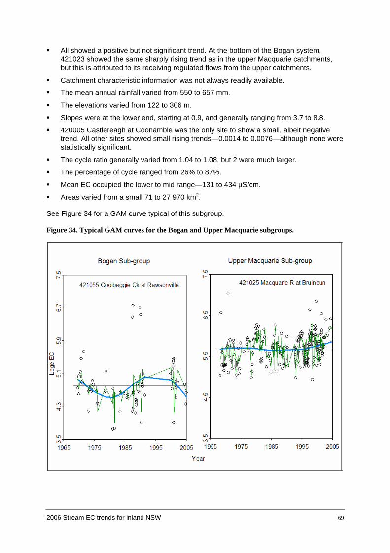
All showed a positive but not significant trend. At the bottom of the Bogan system, 421023 showed the same sharply rising trend as in the upper Macquarie catchments, but this is attributed to its receiving regulated flows from the upper catchments.
Catchment characteristic information was not always readily available.
The mean annual rainfall varied from 550 to 657 mm.
The elevations varied from 122 to 306 m.
Slopes were at the lower end, starting at 0.9, and generally ranging from 3.7 to 8.8.
420005 Castlereagh at Coonamble was the only site to show a small, albeit negative trend. All other sites showed small rising trends—0.0014 to 0.0076—although none were statistically significant.
The cycle ratio generally varied from 1.04 to 1.08, but 2 were much larger.
The percentage of cycle ranged from 26% to 87%.
Mean EC occupied the lower to mid range—131 to 434 µS/cm.
Areas varied from a small 71 to 27 970 km2.
See Figure 34 for a GAM curve typical of this subgroup.
Figure 34. Typical GAM curves for the Bogan and Upper Macquarie subgroups.
2006 Stream EC trends for inland NSW 69

6.1.5 Warrumbungle subgroup 419027 Mooki at Breeza (adjusted dataset)
419072 Baradine Creek at Kienbri (adjusted dataset)
420010 Wallumburrawang Creek at Bearbung
420017 Castlereagh at Hidden Valley
The purpose behind the grouping is described in Section 5.3.2. Essentially the 4 stations had high positive EC trends, but contrary to the norm, also had high average slopes. What linked them was the proximity of 3 of them, and the fact that all were influenced by the Warrumbungle and Liverpool ranges.
General characteristics:
The mean annual rainfall range was narrow, varying from 688 to 762 mm.
Elevations ranged from 282 to 420 m, the 2 Namoi sites being lower.
All linear EC trends were positive, ranging from 0.0056 to 0.0127.
The 4 sites had high slopes ranging from 9.43 to 16.04.
The cycle ratio ranged from 1.04 to 1.08.
The percentage of cycle varied from 26% to 52%.
The recovery factor range was 0.70 to 0.80.
The 4 sites responded to Model 5, with the Namoi valley site R2s being large enough to match the Model 5 range of the Southern Trending subgroup.
See Figure 35 for a GAM curve typical of this subgroup.
2006 Stream EC trends for inland NSW 70

Figure 35. Typical GAM curves for the Warrumbungle and Central Macquarie subgroups.
6.1.6 Namoi and Gwydir valleys and Border Rivers (adjusted datasets)
See Figure 36 for GAM curves typical of the 3 Northern valleys.
With the exception of the 2 sites in the Warrumbungle subgroup, the northern sites do not seem to reflect the dramatic rises noted in the Central Macquarie and Southern Trending subgroups. To a small extent, the situation may be driven by the adjustment of 10% made on the earlier data (Annexure A), which diminished the slope coefficients.
The 10% adjustment did not seem to make much statistical difference in the identification of any catchment with a salinity problem. For 12 of the northern catchments, the sign of the slope changed from positive to negative. Before and after the adjustment, the slope was statistically insignificant. These 12 became the basis for the Northern Insignificant subgroup (Section 6.1.6.2).
6.1.6.1 Northern Falling subgroup (8)
These 8 have significantly falling trend slopes after the 10 percent adjustment. Trends at 4 sites (marked ‘*’) were falling and statistically significant before the data adjustment.
416008 Beardy River at Haystack *
418005 Copes Creek at Kimberley
418014 Gwydir River at Yarrowyck
2006 Stream EC trends for inland NSW 71

418025 Halls Creek at Bingara *
418027 Horton River at Dam Site *
419005 Namoi River at North Cuerindi
419016 Cockburn River at Mulla Crossing *
419029 Halls Creek at Ukolan
General characteristics:
Mean annual rainfall varies from 779 to 912 mm.
The elevations generally range from 313 to 454 m, but 2 sites are much higher: Gwydir at Yarrowyck (738 m) and Copes at Kimberley (756 m).
The log space trend slopes range from –0.0044 to –0.0183 and are significant.
Recovery factors range from 1.08 to 1.69 (Horton River at the Dam Site).
Cycle ratios generally range from 1.02 to 1.04, with the highest being 1.10.
Cyclicity varies 12% to 33%, Horton at the Dam Site being 54%.
Average catchment slopes vary from 5.32 to 13.8. Two sites have catchment slopes that are smaller than normally associated with a falling trend: Copes Creek at Kimberley (5.3) and Gwydir at Yarrowyck (5.5).
The mean EC generally ranged from 178 to 669 µS/cm, with 418025 Halls Creek at Bingara a comparatively high 1039 µS/cm.
Catchment areas ranged from 171 to 2524 km2.
In viewing the various outputs, 2 points are worth noting. Halls Creek at Bingara had a very poor relationship between EC and flow, and a very poor fit of the flow component of the Model 7 curve (Appendix 2.54). In the Namoi River at North Cuerindi (Appendix 2.59), the later record has a long gap of a decade, followed by a group of 7 points. An additional year of samples would increase our confidence in this result. Beardy River at Haystack (Appendix 2.35) has 2 characteristics worthy of note. The EC was rising steeply at the start of its record, and it shares with Horton River at Dam Site (Appendix 2.55) a very pronounced cycle in comparison with the rest of the subgroup.
6.1.6.2 Northern Insignificant subgroup (16)
When the data correction was applied to the Northern record, 12 sites changed sign from positive to negative, but the trend slopes remained statistically insignificant. Of the 12, 3 had a slope very close to zero before the adjustment. A further 6 sites marked ‘*’ had a negative, insignificant loge trend both before and after the adjustment:
416003 Tenterfield Creek at Clifton
416010 Macintyre River at Wallangra*
416016 Macintyre River at Inverell
416023 Deepwater Creek at Bolivia
416027 Gil Gil Creek at Weemalah *
416032 Mole River at Donaldson*
418015 Horton River at Rider (Killara)
418016 Warialda Creek at Warialda
2006 Stream EC trends for inland NSW 72

418017 Myall River at Molroy
418018 Keera Creek at Keera
418032 Tycannah Creek at Horseshoe Lagoon.
418052 Carole Creek near Garah *
419032 Coxs Creek at Boggabri *
419033 Coxs Creek at Tambar Springs
419035 Goonoo Goonoo Creek at Timbumburi
419051 Maules Creek at Avoca East.
419053 Manilla River at Black Springs
419054 Swamp Oak Creek at Limbri *
General characteristics:
Mean annual rainfall ranges from 556 to 899 mm.
Elevation generally ranges from 159 to 655 m, with 416023 Deepwater at Bolivia a relatively high 783 m.
The loge trend slopes are insignificant and range from –0.0007 to –0.0071 (419032 Coxs Creek at Boggabri).
The recovery factors generally range from 0.92 to 1.10; 419032 Coxs Creek at Boggabri has a value of 1.33.
The cycle ratio at 15 of the sites ranges between 1.01 and 1.04. 419032 Coxs Creek at Boggabri shows 1.09.
The cyclicity generally varies from 6% to 35%. Once more 419032 Coxs Creek at Boggabri is at the extreme, at 52%.
Two catchments slopes are very flat: 418016 Warialda Creek at Warialda, with an average slope of 3.8, and 418016 Myall River at Molroy, with a slope of 4.4. The remainder vary between 6.8 and 15.7.
The mean EC ranges between 152 and 1092 µS/cm.
The areas range between 152 and 3803 km2.
The hypsometric integrals range between 0.174 and 0.508.
Most sites have no serious issue in relation to sparse data after long gaps. At 2 sites, greater confidence could be drawn when more data points are added to the later record: 419035 Goonoo Goonoo Creek at Timbumburi and 419054 Swamp Oak Creek at Limbri. Perhaps there is enough evidence for 419032 Coxs Creek at Boggabri to be placed in another subgroup.
2006 Stream EC trends for inland NSW 73

6.1.6.3 Northern Rising subgroup (8)
Figure 36. Typical GAM curves for the 3 northern valleys.
Eight sites showed a rising trend both before and after the 10% adjustment. At 3, the trend was still significant after the adjustment; at 3 others (in the upper Gwydir) it became insignificant (‘*’) after the adjustment:
416020 Ottleys Creek at Coolatai
416021 Frazers Creek at Ashford
416039 Severn River at Strathbogie
417001 Moonie River at Gundablouie
418008 Gwydir River at Bundarra
418021 Laura Creek at Laura *
418023 Moredun Creek at Bundarra *
418029 Gwydir River at Stoneybatter *
General characteristics:
The mean annual rainfall ranges between 743 and 880 mm.
Most of the site elevations range between 346 and 723 m. 417001 Moonie River at Gundablouie is much lower, at 149 m.
The catchment slopes are all <7.8.
2006 Stream EC trends for inland NSW 74

The loge space EC trends are all positive, and range between 0.0004 and 0.0081. Three of these are statistically significant, even after the adjustment: 416021 Frazers Creek at Ashford, 416039 Severn River at Strathbogie and 418008 Gwydir River at Bundarra.
The percentage of cycle varies from 4.5% to 45% (Frazers Creek at Ashford).
The cycle ratio ranges from 1.01 to 1.08.
The mean EC range is tight: 141 to 433 µS/cm, except 416020 Ottleys Creek at Coolatai at 724 µS/cm.
Most areas range from 344 to 4048 km2, except Moonie at Gundablouie at 15,810 km2.
6.2 Catchment characteristics as an explanation of trend
The subgroups of Section 6.1 and Table 5 were a convenient starting point in trying to relate salinity trends to catchment characteristics. If relationships can be found, then it may be possible to use the characteristics to infer rising salinity trends at catchments where there is no EC monitoring. Figures 37 to 42 were used to seek out any such patterns. The following work is a diagrammatic presentation of Table 5, but is based on the assumption that the processes at the collection sites are representative of the catchment above. This is not always the case. The groups were colour-coded based on whether their constituents were seen as not having a short-term problem (green) or having a major problem (red). The colour coding was subjective, but is convenient for viewing. For example, the Lachlan Rising and Northern Rising were both colour coded yellow, although they were known to have a rising trend (Figure 37).
The first step involved revisiting the mean annual rainfall vs site elevation graph of Figure 27. 417001 Moonie River at Gundablouie has not been included in Figure 37 because the rainfall data were not readily available. Five sites in the remaining Northern Rising subgroup are higher than 640 m, and receive modest rainfall in excess of 770 mm per year. The northern group is at odds with rising trend catchments in the rest of the State. As can be seen from the marked lines, most of the problem sites have outlets bounded below 825 mm rainfall and below 430 m altitude. In summarising Figure 37, the 800 mm rainfall could be used as a defining boundary that separates the problem sites from the falling trend site at outlet elevations below 600 m. For the catchments above 430m, there is no defining rainfall boundary.
2006 Stream EC trends for inland NSW 75

Figure 37. Catchment groups relative to mean annual rainfall and elevation.
Elevation at the gauge (m)
200 400 600 800
Ann
ual r
ainf
all (
mm
)
400
600
800
1000
1200 Central Macquarie (5)Southern Trending (10)Warrumbungles (4)
Lachlan rising (9)Northern rising (8)Bogan (7)
Upper Macquarie (8)
Northern falling (8)
Lachlan mountains (3)
Northern insignificant (18)
Upper Murrumbidgee (6)
Snowy (6)
Figure 38. Catchment groups relative to linear trend and gauge elevation.
Elevation at the gauge
200 400 600 800
Line
ar tr
end
coef
ficie
nt
-0.02
-0.01
0.00
0.01
0.02
0.03
Central Macquarie (5)Southern Trending (10)Warrumbungles (4)
Lachlan rising (9)Northern rising (8)Bogan (7)
Upper Macquarie (8)
Northern falling (8)
Lachlan mountains (3)
Northern insignificant (18)
Upper Murrumbidgee (6)
Snowy (6)
2006 Stream EC trends for inland NSW 76
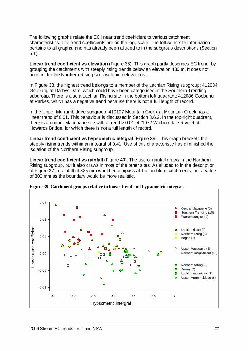
The following graphs relate the EC linear trend coefficient to various catchment characteristics. The trend coefficients are on the loge scale. The following site information pertains to all graphs, and has already been alluded to in the subgroup descriptions (Section 6.1).
Linear trend coefficient vs elevation (Figure 38). This graph partly describes EC trend, by grouping the catchments with steeply rising trends below an elevation 430 m. It does not account for the Northern Rising sites with high elevations.
In Figure 38, the highest trend belongs to a member of the Lachlan Rising subgroup: 412034 Goobang at Darbys Dam, which could have been categorised in the Southern Trending subgroup. There is also a Lachlan Rising site in the bottom left quadrant: 412086 Goobang at Parkes, which has a negative trend because there is not a full length of record.
In the Upper Murrumbidgee subgroup, 410107 Mountain Creek at Mountain Creek has a linear trend of 0.01. This behaviour is discussed in Section 8.6.2. In the top-right quadrant, there is an upper Macquarie site with a trend > 0.01: 421072 Winburndale Rivulet at Howards Bridge, for which there is not a full length of record.
Linear trend coefficient vs hypsometric integral (Figure 39). This graph brackets the steeply rising trends within an integral of 0.41. Use of this characteristic has diminished the isolation of the Northern Rising subgroup.
Linear trend coefficient vs rainfall (Figure 40). The use of rainfall draws in the Northern Rising subgroup, but it also draws in most of the other sites. As alluded to in the description of Figure 37, a rainfall of 825 mm would encompass all the problem catchments, but a value of 800 mm as the boundary would be more realistic.
Figure 39. Catchment groups relative to linear trend and hypsometric integral.
Hypsometric intergral
0.1 0.2 0.3 0.4 0.5 0.6 0.7
Line
ar tr
end
coef
ficie
nt
-0.02
-0.01
0.00
0.01
0.02
0.03
Central Macquarie (5)Southern Trending (10)Warrumbungles (4)
Lachlan rising (9)Northern rising (8)Bogan (7)
Upper Macquarie (8)
Northern falling (8)
Lachlan mountains (3)
Northern insignificant (18)
Upper Murrumbidgee (6)
Snowy (6)
2006 Stream EC trends for inland NSW 77
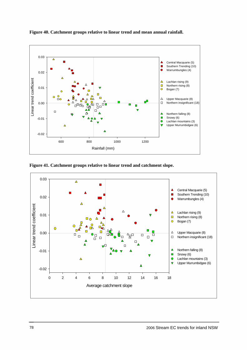
Figure 40. Catchment groups relative to linear trend and mean annual rainfall.
Rainfall (mm)
600 800 1000 1200
Line
ar tr
end
coef
ficie
nt
-0.02
-0.01
0.00
0.01
0.02
0.03
Central Macquarie (5)Southern Trending (10)Warrumbungles (4)
Lachlan rising (9)Northern rising (8)Bogan (7)
Upper Macquarie (8)
Northern falling (8)
Lachlan mountains (3)
Northern insignificant (18)
Upper Murrumbidgee (6)
Snowy (6)
Figure 41. Catchment groups relative to linear trend and catchment slope.
Average catchment slope
0 2 4 6 8 10 12 14 16 18
Line
ar tr
end
coef
ficie
nt
-0.02
-0.01
0.00
0.01
0.02
0.03
Central Macquarie (5)Southern Trending (10)Warrumbungles (4)
Lachlan rising (9)Northern rising (8)Bogan (7)
Upper Macquarie (8)
Northern falling (8)
Lachlan mountains (3)
Northern insignificant (18)
Upper Murrumbidgee (6)
Snowy (6)
2006 Stream EC trends for inland NSW 78

Linear trend coefficient vs average catchment slope (Figure 41). This figure suggests that catchment slope (expressed as an angular measure), may explain EC trend. The vertical line represents a slope of 8.4°. The upper left quadrant contains all the rising trend sites except the Warrumbungle subgroup and the 2 sites 410107 and 421072 already alluded to in this section. The graph implies that rising trend is usually associated with flat catchments. With the exception of the Warrumbungle subgroup, the converse is also true—that steep slopes are not associated with severe rising EC trend.
In one way the Warrumbungle subgroup is the exception: its average slopes are steep. In another way it is not the exception: the average slope incorporates an upper catchment that is very steep and a lower catchment that is very flat. It is probably the lower half of the catchment that is controlling the salinity behaviour.
Percentage of cycle versus hypsometric integral (Figure 42). The cyclic nature of the GAM curves is important in understanding the catchment EC process. The time span (and the amplitude) associated with the full cycle at a site has a big influence on the linear EC trend calculations. In this context, we tried to relate catchment characteristics to the cyclic parameters. Figure 42 does not suggest any concise relationships. Most of the problem sites seem to be contained within the bounds of 25% of the cycle and a hypsometric integral < 0.41. But Figure 42 doesn’t provide an explanation for catchments with a falling trend.
Figure 42. Catchment groups relative to percentage of cycle and hypsometric integral.
Hypsometric integral
0.0 0.1 0.2 0.3 0.4 0.5 0.6 0.7
% o
f cyc
le
0
20
40
60
80
100
Central Macquarie (5)Southern Trending (10)Warrumbungles (4)
Lachlan rising (9)Northern rising (8)Bogan (7)
Upper Macquarie (8)
Northern falling (8)
Lachlan mountains (3)
Northern insignificant (18)
Upper Murrumbidgee (6)
Snowy (6)
2006 Stream EC trends for inland NSW 79

7 Ancillary Investigations
7.1 Modelling base flow separately
Most samples had been taken during base flow sequences (Section 3.2). However, we were concerned that the inclusion of a (comparatively small) number of event samples might be affecting the trend results. As part of a sensitivity test, we isolated base flow data sets for 10 of the southern sites by using the separation method described in Harvey and Jones (2001).
Model 7 was run using the base flow datasets, and we compared the outputs with the study results that used all the data. Figures were prepared showing plots of the full data set versus the base flow. The linear coefficient was included as slope, as were the number of data points in each sample. Figure 43 compares 412028 Abercrombie River at Abercrombie. All 10 sites are presented in Appendix 3.
Figure 43. Comparison of all data with base flow data only.
The results were tabulated (Table 6), mainly to see whether the slope changed by much in magnitude, sign or statistical significance. The statistical significance was also tabulated to show any change. The plots in Appendix 3 were used to confirm that the GAM curves were similar in both data sets. We deemed the difference between the summary statistics and the fitted spline curve for the pairs of data sets to be minimal.
2006 Stream EC trends for inland NSW 80

2006 Stream EC trends for inland NSW 81
Table 6. Comparison of linear coefficients of all data and base flow data.
Station Station All data Significant Baseflow SignificantNumber Name Slope If <0.01 Slope If <0.01412028 Abercrombie R at Abercrombie -0.0023 0.1763 -0.0029 0.1001410097 Billabong Ck at Aberfeldy 0.0109 0.0000 0.0113 0.0000410061 Adelong Ck at Batlow Rd -0.0008 0.6015 -0.0018 0.2606410038 Adjungbilly Ck at Darbalara -0.0015 0.5657 0.0008 0.8025401013 Jingellic Ck at Jingellic -0.0007 0.4123 -0.0004 0.6642410025 Jugiong Ck at Jugiong 0.0195 0.0000 0.0172 0.0000401009 Maragle Ck at Maragle 0.0007 0.6933 0.0004 0.8704410044 Muttama Ck at Coolac 0.0112 0.0000 0.0100 0.0001410047 Tarcutta Ck at Old Borambola 0.0127 0.0000 0.0117 0.0000410091 Billabong Ck at Wallbundrie 0.0195 0.0000 0.0216 0.0000
Note: The yellow shading signifies statistical non-significance. The brown shading indicates a change in sign of the EC trend at 410038.
7.2 Groundwater pilot study
7.2.1 Scope
If the bore data archive had been packaged in a more accessible way, the groundwater data would have been routinely included in the project.
We chose 8 sites to test the hypothesis that the deep aquifers may have been contributing to the long-term trend. We intended to link water level data from deep bores with the gauging station data. We encountered 2 obstacles in making that link:
It was preferable that the gauging station and the bore both be surveyed to the same datum. (If the bore was not connected to a datum, we estimated the bore surface level from topographic maps. This was not a satisfactory solution.)
The bore data were collected infrequently and were not synchronised with the stream data. Therefore, it was necessary to interpolate the bore data to match the time of the EC sampling. This process would not effectively track minor fluctuations in the water table, but should be adequate to track long-term groundwater trends.
7.2.2 Bore data preparation
At each of the 8 sites, the steps were as follows:
The bore datum was expressed as height in metres (AHD).
A group of ‘nearby’ deep bores was selected, and the observed water table height data were plotted against time. A representative bore was picked from each group (Kyeamba at Ladysmith was an exception to this process).
The data at each representative bore were then interpolated to produce hourly data.
The bore data were then matched against the equivalent stream EC and flow.
7.2.3 Presentation of groundwater results
As can be seen from Section 5.1, in the main study the 2 equations that generated the most interest were Models 3 and 7. We were interested in the effect of adding a groundwater

component to these models. This was done in the form of a spline of water table heights with 2 df. Models 3a and 7a have the groundwater component added (Figure 13).
Model 3a: logeEC ~ s(logeflow, 2) + cost + sint + s(groundwater, 2)
Model 7a: logeEC ~ s(logeflow, 2) + cost + sint + s(yrfrac, 4) + s(groundwater, 2)
The addition of the groundwater component was tracked using 2 approaches. First, we plotted the flow-adjusted EC against the groundwater level data to examine the strength of the relationship. A LOWESS smoothing curve was used to reveal the shape of this relationship. This graph also plotted the flow-adjusted EC against time. These plots are presented in Appendix 4.
Secondly, Table 7 presents summary statistics from fitting these new models. We subjectively compared the differences in R2 from the previous models to ascertain whether the inclusion of groundwater gives any improvements in goodness of fit. Future comparisons of these models should allow enough time for a more comprehensive statistical analysis, including testing for statistical significance of the reduction in residual sums of squares due to additional components, in the usual manner for model-building exercises.
Two decisions are worthy of note:
Near 410048 Kyeamba at Ladysmith, the bores of interest are not surveyed to a datum. The nearest suitable bores were several kilometres away. We chose one west of O’Briens Creek because its behaviour better matched the stream EC plot of 410048 in Appendix 2.
The first attempt at Tarcutta produced a confusing plot (Appendix 4-3a). We decided to remove the 8 bore readings at the lower end of the dataset on the assumption that the water table would have been too low to influence the stream—they were well below the gauging station gauge zero level of 190.7 m AHD. The new graph appeared more realistic (Appendix 4-3b).
Table 7. Impact on R2 of adding a groundwater component (shaded columns).
1 2 3 4 5 6 7 8 9 10 11 12 13 14 15 16
Stat
ionN
o.
Station Name Sta
rt S
tream
EC
End
Stre
am E
C
Mod
el 1
Mod
el 2
Mod
el 3
Mod
el 3
a
Mod
el 4
Mod
el 5
Mod
el 6
Mod
el 7
Mod
el 7
a
Sta
rt G
roun
dwat
er D
ata
End
Gro
undw
ater
Dat
a
Rep
rese
ntat
ive
Bor
e
Dat
um
410091 Billabong Ck at Walbundrie 1969 2003 0.85 0.85 0.85 0.87 0.06 0.07 0.86 0.86 0.87 1979 2003 025133 Ass.410097 Billabong Ck at Aberfeldy 1969 2003 0.47 0.49 0.5 0.52 0.08 0.12 0.53 0.57 0.58 1969 2003 025352 AHD410047 TarcuttaCk. at Old Borambola 1967 2003 0.34 0.34 0.35 0.39 0.19 0.33 0.46 0.61 0.62 1974 2003 030385 AHD
TarcuttaCk at Old Borambola # 1967 2003 0.28 0.28 0.29 0.38 0.21 0.33 0.41 0.58 0.59 1974 2002410048 Kyeamba Ck at Ladysmith 1970 2003 0.56 0.57 0.59 0.75 0.29 0.32 0.68 0.75 0.77 1973 2002 030355 Ass.419027 Mooki R at Breeza 1970 2004 0.19 0.20 0.22 0.39 0.12 0.18 0.30 0.45 0.58 1970 2004 030002 AHD419032 Coxs Ck at Boggabri 1969 2004 0.06 0.08 0.09 0.27 0.02 0.10 0.10 0.38 0.41 1983 2004 036433 AHD419033 Coxs Ck at Tambar Springs 1969 2004 0.51 0.52 0.53 0.57 0.01 0.09 0.53 0.61 0.66 1986 2004 036599 AHD419051 Maules Ck at Avoca 1972 2004 0.15 0.15 0.21 0.35 0.00 0.08 0.17 0.39 0.41 1972 2004 030130 AHD
# Eight data points removed. Ass. = Assumed
At 5 of the 8 sites, the record length had to be shortened to match the bore data record. Columns 1 and 2 show the stream EC record details. These should be compared with columns 13–16, which list the bore record period, the bore number, and whether the bore
2006 Stream EC trends for inland NSW 82

has been surveyed into AHD or an assumed datum. (The length of the bore data record determined the values in Table 7.)
Comparison of Models 3 and 3a (Columns 5 and 6)
The addition of a groundwater component produced a big improvement at 3 of the 4 Namoi sites (4190--), and only marginal improvement at Tambar Springs. It also gave an improvement at Kyeamba at Ladysmith, but this could be due to the subjective choice of the representative bore.
Comparison of Model 3a Columns 6 and 11
This comparison looked at the impact of substituting the time trend component of EC with a ground water component. If the values in Columns 6 and 11 were in close agreement and were noticeably larger than that in Column 5, then the groundwater might equally explain the observed variation in EC. Using this approach, we might infer from Table 7 that the representative bores could equally explain much of the stream EC trend at Kyeamba Creek at Ladysmith, Mooki River at Breeza, Coxs Creek at Boggabri and Maules Creek at Avoca.
Comparison of Models 7 and 7a (Columns 11 and 12)
A difference in these statistics suggests that any EC trend is not entirely explained by the groundwater behaviour. At Mooki River at Breeza, groundwater appears to explain additional variation over and above that explained by flow, seasonality and time.
We checked whether the water table was higher than stream gauge zero level. Unfortunately, it was not. At least 2 sites showed promise of a ground water table connection—419027 Mooki River at Breeza (282.6 m) and 419032 Coxs Creek at Boggabri (242.9 m). At 419027, the table was 2 to 3 m below the gauge zero, and at 419032 the water table was not remotely close.
The 419027 site warranted closer scrutiny. Model 7a registers a groundwater component response, so we conclude that a stream–groundwater interaction is occurring upstream of the gauging station. The likely source is located several kilometres upstream. An extensive perched aquifer to the west of the Mooki (Figure 44) (pers. comm. D. Berhane 2006, DWE, Barwon Region) is a source of some very high EC readings. This perched table appears to be influencing the EC behaviour of Mooki River at Breeza. The outcome suggests that the inclusion of Models 3a and 7a could be used as indicators of upstream ‘point-source’ groundwater intrusion.
Had the groundwater table been above the gauge zero level, there would have been firm support for the use of Models 3a and 7a. The fact that the water table wasn’t as high diminishes the strength of the argument. The possibility that the water table gradient is steeper than the stream bed leads to the possibility of upstream encroachments, as confirmed at the Mooki. Generally speaking, there is also a chance of interactions in some of the deeper stream pools. If bore data nearer the aquifer than the gauging station had been used, a better fit for Models 3a and 7a might have been obtained.
2006 Stream EC trends for inland NSW 83
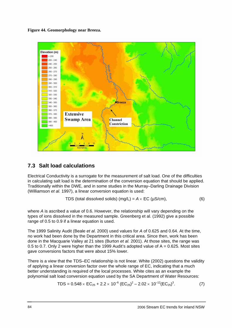
Figure 44. Geomorphology near Breeza.
7.3 Salt load calculations
Electrical Conductivity is a surrogate for the measurement of salt load. One of the difficulties in calculating salt load is the determination of the conversion equation that should be applied. Traditionally within the DWE, and in some studies in the Murray–Darling Drainage Division (Williamson et al. 1997), a linear conversion equation is used:
TDS (total dissolved solids) (mg/L) = A × EC (µS/cm), (6)
where A is ascribed a value of 0.6. However, the relationship will vary depending on the types of ions dissolved in the measured sample. Greenberg et al. (1992) give a possible range of 0.5 to 0.9 if a linear equation is used.
The 1999 Salinity Audit (Beale et al. 2000) used values for A of 0.625 and 0.64. At the time, no work had been done by the Department in this critical area. Since then, work has been done in the Macquarie Valley at 21 sites (Burton et al. 2001). At those sites, the range was 0.5 to 0.7. Only 2 were higher than the 1999 Audit’s adopted value of A = 0.625. Most sites gave conversions factors that were about 15% lower.
There is a view that the TDS–EC relationship is not linear. White (2002) questions the validity of applying a linear conversion factor over the whole range of EC, indicating that a much better understanding is required of the local processes. White cites as an example the polynomial salt load conversion equation used by the SA Department of Water Resources:
TDS = 0.548 × EC25 + 2.2 × 10⁻⁶ (EC25)2 – 2.02 × 10⁻¹²(EC25)3. (7)
2006 Stream EC trends for inland NSW 84

It is possible that by the time the salt load modelling is undertaken for this study, there will be a much better knowledge of salt load conversion in at least 2 of the NSW valleys. If the information is readily available, attempts should be made to use it.
7.4 Year of peak
Model 7 GAM curves (Appendix 2) were inspected to determine the year of highest GAM EC at each station. The results suggest that the timing of the phases varied across the State. We were interested to know whether the EC peak was operating like a pulse in each valley, occurring later as it moved down the valley. Figure 45—Elevation versus year of GAM peak—was plotted to test this. The Macquarie and Castlereagh sites were not included because of the current sharp upward trend at many sites in these valleys.
Murrumbidgee Valley sites plus Maragle
No estimate of year of peak could be made for 410045 Billabung at Sunnyside. At the 12 remaining sites, the peaks ranged from 1978 to an estimated peak at 2002, a span of at least 18 years. Figure 45 suggests that the mid Murrumbidgee is still draining out—at least at the sites that were used in this report. The plots of the various catchment characteristics suggest that the EC trend takes longer to stabilise and fall if the catchment has a low outlet elevation.
401013 Jingellic Creek at Jingellic peaked much earlier than the Murrumbidgee sites (including Maragle Creek at Maragle). At all the Murrumbidgee–Murray sites with comparable record lengths, Jingellic is the only site where the GAM plot (Appendix 2.2) has gone through a trough and is starting to rise again. Is this behaviour a precursor for other sites?
Lachlan Valley
It was difficult to discern a peak, let alone any pattern, at many of the sites in this valley. The peaks occurred over 1991 to 1996, with little evidence of outlet elevation having an influence.
Macintyre Valley
No convincing pattern was discernible. Seven catchments peaked between 1977 and 1981, with the more westerly catchment (Gil Gil at Weemalah) lagging behind as late as 1984. Two catchments seemed grossly at odds with the others: 416020 Ottleys Creek at Coolatai and 416039 Severn at Strathbogie. It may be that their behaviour is heralding a new pulse or a new local issue.
Gwydir Valley
No convincing pattern was discernible. The range of years was 1977 to 1985.
Namoi Valley
The Namoi appears to have some similarity with the Murrumbidgee–Murray. The upper catchments appeared to have peaked much earlier (1972 to 1981) than 3 of the lower-elevation catchments (1995–2000).
7.4.1 Tardiness of GAM peak
The Murrumbidgee peaks, and to a lesser extent the Namoi Valley peaks, appear to be moving westward. The Gwydir and Macintyre generally seem to have peaked over 1977 to 1984. The Lachlan peaked from 1991 to 1996.
2006 Stream EC trends for inland NSW 85
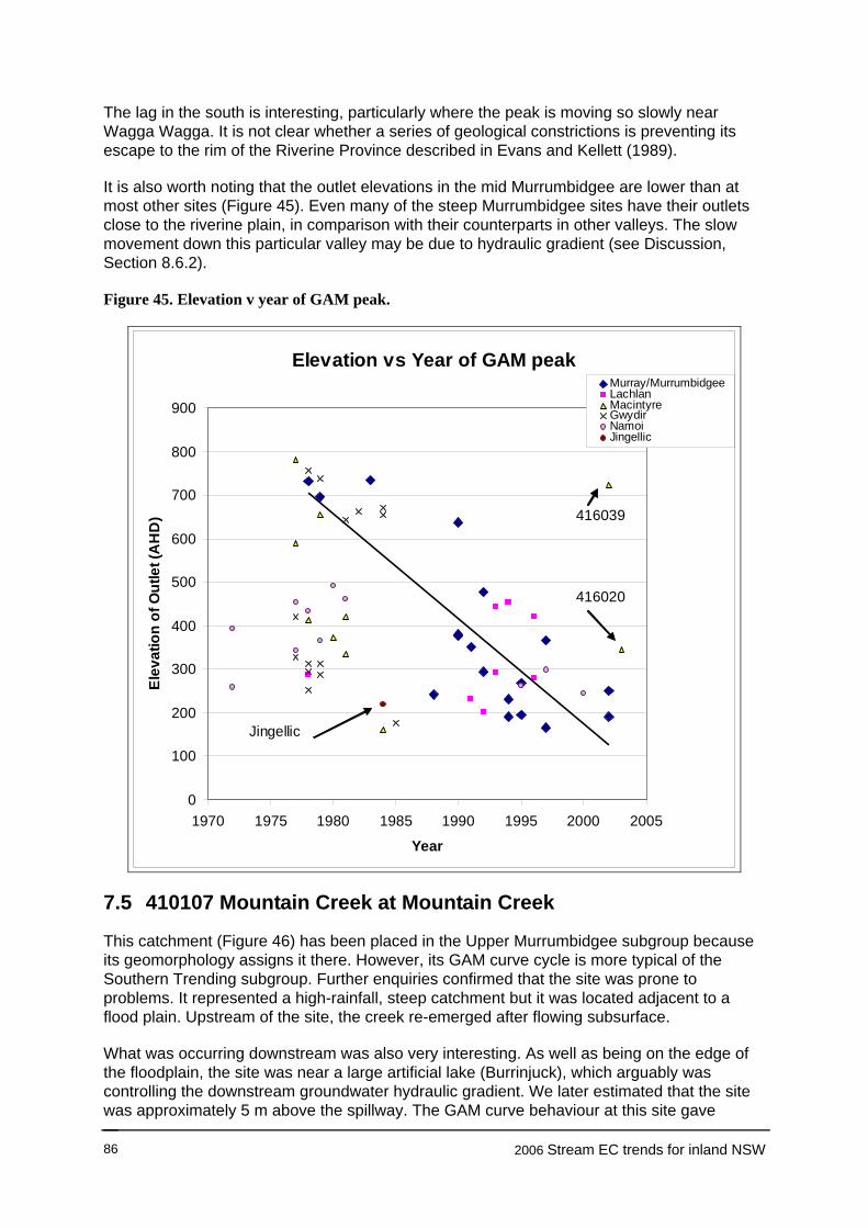
The lag in the south is interesting, particularly where the peak is moving so slowly near Wagga Wagga. It is not clear whether a series of geological constrictions is preventing its escape to the rim of the Riverine Province described in Evans and Kellett (1989).
It is also worth noting that the outlet elevations in the mid Murrumbidgee are lower than at most other sites (Figure 45). Even many of the steep Murrumbidgee sites have their outlets close to the riverine plain, in comparison with their counterparts in other valleys. The slow movement down this particular valley may be due to hydraulic gradient (see Discussion, Section 8.6.2).
Figure 45. Elevation v year of GAM peak.
Elevation vs Year of GAM peak
0
100
200
300
400
500
600
700
800
900
1970 1975 1980 1985 1990 1995 2000 2005
Year
Elev
atio
n of
Out
let (
AH
D)
Murray/MurrumbidgeeLachlanMacintyreGwydirNamoiJingellic
Jingellic
416020
416039
7.5 410107 Mountain Creek at Mountain Creek
This catchment (Figure 46) has been placed in the Upper Murrumbidgee subgroup because its geomorphology assigns it there. However, its GAM curve cycle is more typical of the Southern Trending subgroup. Further enquiries confirmed that the site was prone to problems. It represented a high-rainfall, steep catchment but it was located adjacent to a flood plain. Upstream of the site, the creek re-emerged after flowing subsurface.
What was occurring downstream was also very interesting. As well as being on the edge of the floodplain, the site was near a large artificial lake (Burrinjuck), which arguably was controlling the downstream groundwater hydraulic gradient. We later estimated that the site was approximately 5 m above the spillway. The GAM curve behaviour at this site gave
2006 Stream EC trends for inland NSW 86
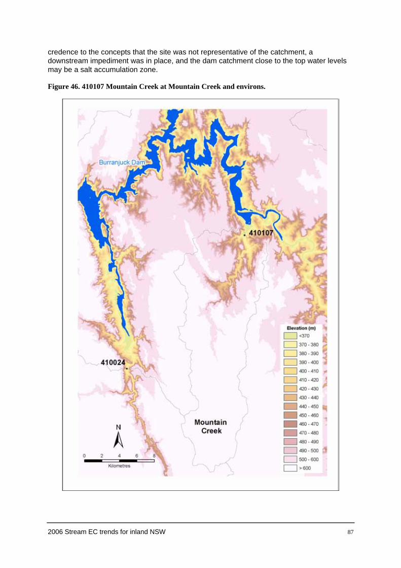
credence to the concepts that the site was not representative of the catchment, a downstream impediment was in place, and the dam catchment close to the top water levels may be a salt accumulation zone.
Figure 46. 410107 Mountain Creek at Mountain Creek and environs.
2006 Stream EC trends for inland NSW 87

8 Discussion
In undertaking such an investigation, not only are the final calculations important, but so too is the level of confidence that can be attributed to them. Much of this section is dedicated to discussing the limitations of each step in the achievement of a final result.
8.1 Limitations in the EC–flow relationship
The relationship between logeEC and loge(instantaneous flow) is the cornerstone of a successful Model 7 fit (Section 5.1). At some sites the relationship was good, whereas at others it was not. There are a number of reasons why the catchment upstream of the gauging station might not exhibit a good correlation.
8.1.1 Catchment processes
8.1.1.1 Catchment heterogeneity
There may be spatial variability in salt supply due to different geologies and different aquifer exposures. Some parts of the catchment may receive higher rainfall. These subcatchments have had greater opportunity for mobilisation over the centuries, and might already be well leached. In contrast, the drier subcatchments will have had comparatively less opportunity for mobilisation, and consequently have more salt available for mobilisation in wetter decades. A high variability in a catchment’s rainfall could point to a high cyclicity, which in turn points to mercurial EC trend behaviour over the long term.
8.1.1.2 Systematic errors in the data
The study has flagged a possible systematic error in the discrete EC data set due to instrument limitations. This is discussed extensively in Annexure A.
Rating tables that are not representative of the stream behaviour can cause systematic errors in the high flow regimes. Sites with poor controls can greatly affect the definition of low flows, and these errors will be magnified by the fact that the calculations are performed in the scale of natural logarithms.
8.1.1.3 Hysteresis
There could be an offset in the relationship between EC and flow between the rising and falling limbs of an event hydrograph (Harvey and Jones 2001). It has implications in the development of EC–flow relationships at high flows. In this study, it may have some negative effects—particularly if there are few data points.
8.1.1.4 Precision of instrumentation
At some of the study sites, the EC range and individual EC values were low. It is conceivable that instrument errors were as large as (if not larger than) the trend being measured.
8.1.1.5 The relationship does not exist
At many sites, particularly in the 3 northern valleys, the EC–flow relationship was poor (Tables 2 and 3, Model 3 column). At 1 other site (410103 Houlaghans at Downside), the statistics of Table 2 point to a good relationship. However, closer scrutiny shows that with just 28 data values spanning 28 years, the EC–flow relationship is weak.
2006 Stream EC trends for inland NSW 88

8.1.2 Choice of equation to explain the EC–flow relationship
Jolly et al. (1997, 2001) relied on the monthly means of EC and flow. Because many of their catchments were large and regulated, this appears the best way to go. Our study deals mainly with tributaries, which would tend to have larger variations in flow and EC. We decided to relate EC to instantaneous flow (Harvey and Jones 2001). This is likely to provide a closer EC–flow relationship, but the ‘flashier’ nature of smaller tributaries could generate other difficulties in the relationship.
8.2 Limitations in the data
Is it possible that the GAM output is describing a process which is different to an EC trend?
Data preparation is described at length in Sections 2 and 3 and in Annexure A. The quality of the EC data is likely to have varied over time. The original collection program may have gone through quality assurance difficulties in the early 1970s, but is likely to have recovered by the late 1970s, and was producing good results through to the early 1990s. A new collection program began by the mid 1990s, but has associated data gaps and ‘teething’ problems. We can expect that the discrete EC data being collected today are gradually improving in quality.
The cyclic nature of the GAM curves (Appendix 2) may be due to:
the collection program itself
the cyclic nature of the tributary flow patterns
decisions made in the data editing of this project.
8.2.1 Data collection program itself
Early record. Annexure A reports possible instrument limitations in the early 1970s. We tried to neutralise the problem in the Macintyre, Gwydir and Namoi, but found insufficient evidence to address the problem in the Lachlan, Murrumbidgee and Murray. The GAM behaviour in the earlier years of record might be explained by data collection problems.
Data gaps. It is not clear how the gap years in the early 1990s might have influenced the model results, particularly at the end of the record. What are an acceptable number and density of sample points to ‘tie down’ the post-gap statistics? One view suggests that trend analyses should not be undertaken if there are gaps, particularly if there are few data points after the gap, because only 1 or 2 data points would have an unacceptable influence on a trend calculation. An opposing view says that the dataset should be analysed, because it can flag possible problems. These unacceptable data points can easily be discarded at a later date if the addition of a dozen or so data points provides contradictory evidence.
Ephemeral streams. At some sites in lower-rainfall zones, streams ceased to flow during a sequence of drier years. It is not clear whether this influences trends in the neighbouring years when there was a record. At other sites, the number of samples fell during drier years because the stream flowed only intermittently. The samples were probably associated with surface runoff, rather than the usual base flow. It is not clear whether this behaviour would cause any bias in the GAM curve, particularly if the dry sequence lasted several years.
Future filling of long data gaps. Our policy was to involve field personnel wherever possible. At the study commencement, we tried to obtain input from various water quality officers concerning the ‘Recent’ dataset. Unfortunately, the work was done at a time of organisational upheaval, and some of the key players were in the process of leaving the
2006 Stream EC trends for inland NSW 89

organisation. This has meant that expert input was not always available during the data editing phase.
As the study progressed and some of the preliminary findings were made known, it became apparent that additional datasets might be available to cover some of the ‘gaps’. This situation appears to be the exception rather than the rule, but it is worth noting for future studies.
8.2.2 Sampling frequency
As alluded to in Section 2.5, we tried to keep the sampling frequency for the ‘recent’ and historical records roughly the same. This was not always easy, but there was a rationale behind it. In generating the data to be used in this technique, we chose a representative flow value: the mean of the logeflow values paired with the EC samples (Appendix 1). Because wetter decades would contain much higher flows than drier decades, it was important to keep the mean logeflow as representative as possible of the field conditions experienced throughout the collection program.
8.2.3 Representative tributary flows
The representative logeflow (referred to in Section 4.6 and listed in Appendix 1) was held constant when the curves in Appendix 2 were generated. We were concerned that this mechanism might distort the trend results. In wetter decades, the representative flow would probably be classified as base flow. In drier cycles, particularly in cases of ephemeral streams, the same flow might be surface runoff—representing a completely different regime of EC. The scenario (of a switch between surface and base flow) is not a probable one, but it should be kept in mind. It provides a good argument for separating the event and base flows with a view to analysing the data sets separately (Section 7.1). Unfortunately there are not enough event data points to perform this operation successfully.
This type of problem is not limited to tributary catchments. It is possibly just as great a problem for sites on regulated streams. During drier years, greater reliance is placed on dam releases. In wetter cycles, the source of flow in the river might be completely different.
8.3 Limitations in the models
The flow spline and the number of degrees of freedom chosen in the time spline might cause limitations. In future studies, there probably needs to be a more flexible approach to handling the number of df chosen in the logeEC–logeflow relationship. At sites with few data points, there needs to be a more flexible df approach in the generation of the GAM trend curve.
a) The flow spline
In some cases, the relationship between logeEC and logeflow was good, but in others it was poor. The spline fits site No. 410091 adequately (Figure 47), but has trouble bending sufficiently to fit either end of the observed flow range at 416010 (Figure 48). When a value of 2 df is not adequately flexible, the time component (in the form of the GAM curve) might try to compensate for any systematic error. If the EC–flow relationship has a high degree of curvature, then the spline will anchor to the mass of points usually at the low end of the flow range. Inflexibility may cause the spline to have difficulty fitting to data points at the high flow end. The question arises as to whether the full model will try to compensate for this high flow/low EC inadequacy by the time spline modelling the inflexibility as a natural fall in EC.
2006 Stream EC trends for inland NSW 90

It is interesting to note that there is generally a poor fit between logeEC and logeflow at the site shown in Figure 48. Not only does the spline function fail to follow the few high flow / low EC events as adequately as one may desire, but a cluster of data at medium flow exhibit quite a broad range of EC values. As can be seen from the fitted curve in Appendix 2.36, both high and low recorded EC values are not modelled well at this site.
The predominance of points in base flow could be biasing high flow results, generally predicting too high. On its own, this is not a problem in the trend analysis, for 2 reasons:
We are interested not so much in the magnitude of an individual value as in how it compares with EC during similar flows in other years.
If the high flow samples occur randomly across time, then it shouldn’t unduly influence the shape of the trend curve.
But a sequence of 3 or 4 wetter years may cause the trend component to compensate for the inflexibility of the flow spline, generating a chronic overestimate in those years and causing a bulge on the GAM curve. If the undulations were solely caused by this statistical weakness, then sites with a predominantly linear EC–flow relationship (i.e. the non-linear component is not significant) should not show undulations. An inspection of a number of relevant sites refuted our concern by revealing undulations.
To address the above concerns, knowledge of EC behaviour at high flows needs to be improved. This in turn emphasises the importance of having confidence in the accuracy of the data, particularly time-series. With future data improvements, consideration could be given to increasing the df of the spline or to separating the dataset into event and base flows.
Figure 47. Adequate spline fit.
2006 Stream EC trends for inland NSW 91

Figure 48. Spline not fitting flow extremes.
b) Degrees of freedom in the time spline
The issue of spline-smoothing is discussed in Section 4.3. At most sites, the choice of 4 df has been appropriate. At sites with comparatively fewer data points, a lower df might be preferable in future.
8.4 Synthesis and cyclicity implications
In viewing the various constraints discussed in Sections 8.1 to 8.3, we need to take into account several major issues. One of the big unknowns in this work pertains to the uncertainty of the systematic errors of the early data sets. Although the impact of the uncertainty may be marginal in a technical sense, it blurs the issue of whether an individual site is experiencing a rising trend or not.
The Model 3 relationship between EC and flow is not always strong. In fact, it is poor at a number of the sites in the northern half of NSW. How this weakness affects accuracy in the trend analysis is uncertain. There appeared to be enough good performances for us to persist with the results. The non-linear component of the GAM curves (Appendix 2) makes trend analysis and forecasting difficult. Therefore, it is important to understand the nature of the cyclic behaviour of the GAM as a prelude to understanding linear trend. By placing emphasis on the cyclic nature of the trends, this study differs from Beale et al. (2000) and Jolly et al. (1997, 2001).
8.4.1 Implications of cyclicity
The subgroups were developed based on similar catchment characteristics and similar GAM curve shapes (Section 6, Figure 30, Table 5) in adjacent catchments. The similarity in subgroup GAM shapes points to climate being the prime driver of cyclic behaviour.
At some sites, the cycle length is shorter than the 30-plus years of data available. In such cases a linear trend has been estimated with a degree of confidence. At other locations, the
2006 Stream EC trends for inland NSW 92

cycle length appears longer than a lifetime (Appendices 2.3, 2.6 and 2.84), and it is much more difficult to understand the processes, because they may never return to the low EC levels of the early 1970s. At other sites, an addition of 10 or so years of data will complete the cycle and enable a much better assessment of long-term trend.
8.4.2 Cycle amplitude and modelling
In some catchments, the cycles are of large amplitude, suggesting the involvement of factors that magnify the climatic fluctuations. Large cycle amplitudes appear to indicate wide characteristic variations within individual catchments—for example, mountains versus plains; wide variations in annual rainfall or water chemistry. It is likely that such characteristics work in combination to magnify the climate fluctuations.
At present, wide variations in catchment characteristics are blurring any evaluation of EC trend. From a modelling perspective, there is need to identify the extent of the catchment variations with a view to disaggregating existing modelled subareas. Modelling that is solely based on existing gauging networks may be inadequate for tracking EC trends. This concept is further supported in Section 8.5.2.
8.5 Geographic subgroups
In Section 6.1, the various catchments have been grouped and linked to geomorphological characteristics (Section 6, Table 5, Figure 30). The subgroups were initially based on proximity and on the similar characteristics that proximity often entails: mean annual rainfall, elevation and slope. We also considered the logeEC trend and cyclic indicators in determining the groupings.
8.5.1 Record length
One complication was record length, which at some sites did not encompass the whole period of record. This resulted in 1 or 2 sites (such as 412086 Goobang at Parkes) seemingly to be grouped incorrectly.
8.5.2 Site location
A second complication pertained to site location. The study was undertaken using data from gauging stations. These sites were originally located to optimise the collection of flow data. Sometimes they were placed in locations that might not be typical of the catchments they represented. For example, in Figures 27 and 38, there is an inference that most members of the Snowy subgroup are located on the river flats at the base of the mountain range. In such cases, there is always the danger that the saline processes being tracked are different from the processes in the mountainous catchments they represent.
This ‘non-representative’ aspect has wider implications. If a stream were traversed from its outlet to the top of its watershed, in most cases the EC magnitude would diminish. The decrease might be gradual, but it could be a step where point-source saline intrusions are crossed. In grouping the catchments, the location of the sampling point should always be kept in mind. The relocation of the site by several kilometres (particularly from river flats to hilly terrain) could effectively change a catchment’s EC reputation.
Examples of non-representative catchments outlets have already been discussed: Tarcutta at Old Borambola (Section 5.3.1), the Warrumbungle subgroup (Section 6.1.5), and specifically Mooki River at Breeza (Section 7.2.3). The implication of location of the outlet gauge is conceptualised in Figure 49.
2006 Stream EC trends for inland NSW 93

Figure 49. Conceptual diagram in Section 8.5.2.
Outlet Gauge on Tableland or Plain, -- Rising Trend
Outlet gauge on Mountainous Catchment, - Trend Equilibrium
Outlet Gauge in River Flats – Trend might be influenced by downstream conditions.
8.5.3 Flat slopes and low outlet elevation
The work in Section 6.2 and Figure 41, which links catchment slope to linear trend, suggests that the EC behaviour may be linked to how effectively the catchment substrata can drain. Catchments with low outlet elevations are likely to have difficulty draining; generally there is no opportunity for saline ground water to escape into lower country downstream. Tableland catchments with low slope could also be subject to drainage difficulties. In Figures 38 and 41, the troublesome subgroups (particularly Southern Trending) fall into the categories of low elevation and flatter slopes. It is possible that other mechanisms are at work, impeding subsurface movement and catchment flushing.
8.6 A conceptual model
The current drought has altered salinity trends. But it has affected the valleys in different ways. For example, the GAM curves for sites in the Murrumbidgee system have generally stopped rising or begun to plummet. In the Macquarie system, the drought has signalled a sharp rise in the GAM curves for the last 10 years. In developing a conceptual model of future behaviour, we must address the impact of the drought consistently. In drawing conclusions and recommendations, we have taken the GAM curve trends for the last 10 years on face value, despite possible extenuating circumstances.
The GAM curves provide little opportunity to forecast to 2020. Modelling is also difficult, because at some sites there is not a sufficiently long data set to evaluate EC behaviour under all hydrological conditions that NSW typically experiences. Careful examination of the GAM curves has led to an assessment of EC processes over the 30+ years of record. Following are some comments about what processes might come into play over the next decade or so.
We have made some fundamental assumptions that any EC peak highlighted in the GAM curves of Appendix 2 will recur or be surpassed sometime in the future. The following
2006 Stream EC trends for inland NSW 94

comments relate to what is likely to happen in the next 20 years, and acknowledge that NSW is still gripped by drought. It is assumed that observed GAM curve peaks can be expected to recur routinely at a particular site.
8.6.1 The ‘episodic’ change and aftermath
In an overview of the GAM curves in NSW, several patterns emerged, suggesting a conceptual model of stream EC behaviour. The various subgroups of Section 6 have highlighted that the following 12 sites showed a sharp increase in EC during the early 1970s. Most of the 12 are located in Jolly et al.’s (2001) ‘Zone 1, Northern–Western Dryland’. It is not clear whether the historical data collection program started after the rising trend began, but the implication seems to be that all 12 sites experienced a sharp EC rise.
The ECs at half the sites were resilient, dropping back to the levels at the start of the collection program, but the remainder dropped only part way back, registering an overall increase (Figure 50). Most sites are in the mid Gwydir Valley, but some are in the Namoi and Border River valleys, and 1 is in the Castlereagh. The catchments are marked ‘E’ in Figure 51. A catchment’s response to the episode often determined its subgroup classification as a rising or falling trend catchment. Generally the steeper catchments returned to the earlier EC levels, whereas the flatter catchments did not. (This behaviour endorses Figure 41 and 49.) Some of the sites listed below have long gaps in their record, but those that haven’t, clearly illustrate the episode’s impact.
416008 Beardy River at Haystack, Appendix 2.35
416021 Frazers Creek at Ashford, Appendix 2.39
418008 Gwydir River at Bundarra, Appendix 2.46
418015 Horton River at Killara, Appendix 2.48
418016 Warialda Creek At Warialda, Appendix 2.49
418017 Myall Creek at Molroy, Appendix 2.50
418018 Keera Creek at Keera, Appendix 2.51
418029 Gwydir River at Stoneybatter, Appendix 2.56
418052 Carole Creek at Near Garah, Appendix 2.58
419053 Manilla River at Black Springs, Appendix 2.67
419054 Swamp Oak Creek at Limbri, Appendix 2.68
420005 Castlereagh River at Coonamble, Appendix 2.72
2006 Stream EC trends for inland NSW 95

Figure 50. Examples of episodic behaviour in Jolly et al.’s Zone 1.
8.6.2 The ‘impeded’ sites
The GAM curves of some sites indicate a long cycle, and it is difficult to assess what the outcome might be at the end of it. These impeded sites encompass the Southern Trending and Warrumbungle subgroups, as well as 410107 Mountain Creek at Mountain Creek. A number of these may ultimately be termed Episodic, as described in Section 8.6.1. It is difficult to see many of the Southern Trending catchments returning to the EC levels of the early 1970s within the next 20 years. Two are trending upward with little respite—410091 Billabong at Walbundrie (Appendix 2.3) and 410025 Jugiong Creek at Jugiong (Appendix 2.6).
Probably as a result of the drought, several Southern Trending sites have started to trend downwards in recent years after prolonged climbs. There are at least two possible reasons for the various behaviours. At Kyeamba Creek at Ladysmith (Appendix 2.13), Tarcutta Creek at Old Borambola (Appendix 2.12), and Muttama Creek at Coolac (Appendix 2.10), the trends might be explained by large variations in annual rainfall across the catchments (see Section 6.1.3).
A second explanation is associated with limited hydraulic gradients or obstruction to groundwater movement, preventing access to the regional groundwater systems. The possibility of constrictions at Mooki at Breeza (Appendix 2.61) is discussed in Section 7.2.3. The Mountain Creek (Appendix 2.20) retardation scenario is discussed in Section 7.5.
2006 Stream EC trends for inland NSW 96

Figure 51. The episodic catchments (‘E’) and catchments of interest (pink).
Flat hydraulic gradients in the groundwater table have implications at a valley scale. The catchments with rising trend are generally associated with low average slopes, whether plains or tablelands (Figure 41).
2006 Stream EC trends for inland NSW 97

The Southern Trending subgroup is perplexing if its behaviour is to be explained by the regional groundwater table. There are a number of study sites in the Bogan, Castlereagh and Border Rivers that are lower than (or at approximately the same AHD as) the Southern Trending sites. However, none are showing significant rising trends or the variation in cyclicity that one would expect of a rising regional water table. It is possible that the causes of the Southern Trending behaviour might be driven by local geographic features, and relate to groundwater hydraulic gradients. There are locations where the various streams and rivers pass through ranges of hills whose geology may constrict groundwater movement. There is the possibility that (at this point in time) the problem might not be caused by the regional water table rising, but rather that the Murrumbidgee, Lachlan and Billabong systems are suffering impeded groundwater movement. Small north–south ranges of hills are the likely impediment. The Malebo Range immediately downstream of Wagga Wagga may be playing some part in impeding the mid Murrumbidgee tributaries. Braaten and Gates (2003) noted that after a large recharge event (1989), it took several years for the groundwater system to drain back into the Wagga–Narrandera section of the Murrumbidgee River.
The evidence for establishing the Warrumbungle subgroup is a little circumstantial. It is based on the extreme variations in the individual catchment characteristics. There is much higher annual rainfall along the narrow mountain strip. This flows down precipitous parts of the catchment and accumulates in the plains below. The water gradually filters into the stream systems, as described for Mooki River at Breeza in Section 7.2.3.
Sites in the Southern Trending subgroup have substantially rising ECs, and the trends are statistically significant. There is no guarantee that some will return to the EC levels of the early 1970s. Members of the Warrumbungle group are experiencing the same rising trends, but not to the same extent.
8.6.3 Subgroups in equilibrium (Table 5 and Figure 52)
These are major contributors to the valley runoff but, in terms of rangeland coverage, occupy only a small portion of the valley catchments.
Snowy subgroup (Section 6.1.1 a)
This group features a mixture of non-significant trends, both positive and negative in sign. No substantial change in behaviour is expected.
Upper Murrumbidgee subgroup (Section 6.1.1 b)
ECs at most of these sites peaked in the late 1970s and maintained that level for a decade before falling in the mid 1990s. They are falling significantly, but would be expected to return to and maintain the higher levels of the late 1970s when the drought finishes.
Lachlan Mountains subgroup (Section 6.1.1 c)
All show a falling trend at present, which is statistically insignificant. The sign of the trend might vary over the years, but no major changes are expected.
Other areas that are likely contenders for the Equilibrium group are most catchments on the northern side of the Namoi Valley. These sites fall within the Northern Falling or Northern Insignificant subgroups.
2006 Stream EC trends for inland NSW 98

Figure 52. Zones in the southern part of NSW.
8.6.4 Rising trend, but insignificant
Upper Macquarie subgroup (Section 6.1.4 a)
All the trends are statistically non-significant. Most are rising, mainly during the last 10 years. Under normal conditions these sites would have been nominated as an Equilibrium subgroup. However, the sharply rising trend over the last decade precludes such a commitment. We advise a wait-and-see policy until the drought is broken.
2006 Stream EC trends for inland NSW 99

Bogan subgroup (Section 6.1.4 c)
ECs at most of these sites have a rising trend which is statistically insignificant. It is of interest that several of these sites have the lowest elevation in the study. But they do not seem to be suffering the extreme impact of the Southern Trending sites.
8.6.5 Rising trend, significant
These subgroups are of grave concern. This category includes the 2 subgroups already identified and discussed in Section 8.6.2:
Southern Trending
Warrumbungles.
The remaining subgroups incorporate 2 tableland areas in the upper Lachlan and upper Gwydir:
Lachlan Rising (Section 6.1.2)
Central Macquarie (Section 6.1.4 b)
Northern Rising (Section 6.1.6.3) plus 2 catchments from the plains: 416027 Gil Gil at Weemalah and 418052 Carole Creek at Near Garah. These 10 catchments (along with 2 of the Warrumbungle sites) are shaded pink in Figure 51.
One aspect that most of these have in common is a low average slope.
8.7 General
8.7.1 Statistically insignificant trends
The fitted GAM plots (Appendix 2) are cyclic and mainly short-term. If the cycle is much longer, the sign of the trend may fluctuate as the record extends. Not much credence can be placed on the fact that the sign is negative. The situation suggests that the sign must have been positive in the past. Statistically insignificant negative trends are treated as being in equilibrium.
8.7.2 Decisions on data adjustment
Annexure A weighs up the need to adjust the early years of data. There was sufficient evidence to make an adjustment of +10% to the data in the northern 3 valleys. The adjustment flattened the trend, and the adjusted slopes have been used in the calculations for this report. At half the 36 sites, the adjustment did not change the sign of the trend. At 12 of the sites, the trend changed from positive to negative. Linear slopes were statistically insignificant in both scenarios.
In the south, no adjustment was adopted, although we suspected that a similar problem existed. Some sensitivity tests were undertaken to see what effect a correction of 15% would have on the results. The problem catchments remained problems, although 5 of the less troublesome catchments slopes changed sign from positive to negative, but remained statistically insignificant.
In the deliberations below, the implications of the adjustments are considered, regardless of whether the changes were made (north) or not (south).
2006 Stream EC trends for inland NSW 100

8.8 Comparison with Jolly et al.’s work
Model 7 and the work done in Jolly et al. (1997, 2001) are generic. Their methods use the same trend spline and seasonality component, although they vary substantially in the way they include flow.
The analysis by Jolly et al. (1997) was based on the monthly means of EC and flow. They applied a flow-weighting based on a monthly flow interval. Because many of their catchments are large and regulated, the monthly interval is a good approach.
We used Model 7 to establish a foundation relationship between EC and instantaneous flow. Tributary catchments were seen as preferable in achieving the foundation, because the EC sampling was likely to be spread more equitably over the flow range, than would be the case with sites on larger (regulated) rivers. Our work provides detail as to how well the model fitted each site.
Jolly et al. (2001) extended the EC trend work to incorporate salt load output–input in various river reaches. (We have not tried to cover this.) They focused on the linear EC trend to describe catchment EC behaviour. They grouped the MDB into 4 zones and based their conceptual model loosely on mean annual rainfall and elapsed time since clearing. We based our trend assessment on the linearity component, but identified the cyclic nature of the trend curve as an important guide to catchment EC behaviour. In concept, our study has sought to provide a link between EC behaviour and catchment geomorphology—mainly catchment slope, but also elevation and shape (hypsometric integral).
Both studies analysed the 7 sites compared in Table 8. We attribute any differences in mean EC to the extra 10 years of data available to us. In 6 of the 7 cases, the new trend values fall within Jolly et al.’s trend bands, although not vice-versa. The GAM plots of Appendix 2 give credence to the differences between the 2 trend values at each site. There is nothing untoward between the 2 sets of values.
Table 8. Comparison with Jolly et al.’s (1997) results at 7 common sites.
Jolly et al. (2001) This study Station No. Station name Mean EC
(µS/cm) Trend
(µS/cm/y) Mean EC (µS/cm)
Trend (µS/cm/y)
416027 Gil Gil Creek at Weemalah 425 5.2 ± 6.7 420 1.1 ± 2.9 417001 Moonie River at Gundablouie 130 4.5 ± 4.6 141 0.1 ± 1.0 420005 Castlereagh River at Coonamble 485 –2.4 ± 4.6 434 –0.4 ± 3.3 421042 Talbragar River at Elong Elong 1050 8.4 ± 11.2 1052 8.8 ± 9.9 421023 Bogan River at Gongolgon 330 –3.0 ± 3.8 347 1.1 ± 2.8 410050 Murrumbidgee River at Billilingra 110 0.1 ± 1.8 100 –0.9 ± 0.6 410091 Billabong Creek at Walbundrie 1300 59.8 ± 34.6 1324 26.1 ± 7.8
8.9 EC forecasting and comparison with 1999 audit
8.9.1 Forecasting to 2020
Originally we proposed to extrapolate the GAM curves to 2020, with a view to providing a forecast for each site. Apart from making the prediction, one of the reasons for doing this was to enable a comparison to be made between this investigation and Beale et al. (2000). There were 3 stages involved in this task, as described in Appendix 5.
2006 Stream EC trends for inland NSW 101

When examining the predecessor of this report, the reviewers indicated that it was statistically unsound to forecast by extending the GAM curve, because the curvature was unique to the observed record.
Forecasting was always going to be difficult. The GAM curves suggested a combination of meteorological, geomorphological and episodic influences; unless the processes driving the EC trends could be identified, then it would be very difficult to achieve predictions for 2020.
We decided to proceed with the forecasting exercise, but only to use sites whose non-linearity was statistically non-significant. Of the 92 sites, only 20 were in this category, the Lachlan and Macquarie systems each accounting for a third of the number. Results are presented in Table 9.
8.9.2 Comparison with 1999 Salinity Audit
The approaches used by the 1999 Audit and this investigation were completely different approaches. Without fully dissecting the 2 approaches, we can show a primary difference which could lead to results that are not comparable. The 1999 Audit calculated an average annual salt load for the MDB Commission Benchmark’s 21 years of data (1975–1995). This average was nominated as representing the 1998 salt load. In reality, it represented the mean for the 21 years: that is, the nominated 1998 value was probably closer to the 1985 value. At many stations, the trends were not large, and there was not going to be much of a difference between the ‘1985’ and 1998 figures. At sites where the trend was large, the average result for the Benchmark years could be vastly different from the real 1998 value.
Because we have emphasised the cyclic character of the trends, our investigation differs from both the 1999 Audit and the work by Jolly et al. At many sites, this approach leads to the conclusion that the linear trends may not be as large as first thought. But at sites that have not gone through a full cycle, interpretation is difficult, and assessment defaults to the linear trend calculation.
The 1999 Audit calculated ratios of the 2020 salt load to the 1998 salt load. We undertook similar calculations for the same period using the EC linear trend results (Table 9). Only 20 sites were useable in this exercise, as explained in Section 8.9.1.
2006 Stream EC trends for inland NSW 102

Table 9. Comparison between this study and 1999 Audit for 2020/1998 EC ratios.
Column 1 No.
Column 2 Station Name
Column 3 Sub-Group Code C
olum
n 4
2020
/199
8 R
atio
Th
is S
tudy
Col
umn
5 20
20/1
998
Rat
io
1999
Aud
it
Col
umn
6
So
urce
- 19
99
Audi
t Tab
les
412050 Crookwell R. at Narrawa North Lachlan Mountains 0.98 1.28 Table 6.9412083 Tuena Ck. At Tuena Lachlan Mountains 0.80 1.30 Table 6.9410026 Yass River at Yass Lachlan Rising 1.19 1.35 Table 6.1412043 Goobang Ck. at Darbys Dam Lachlan Rising 1.87 1.16 Table 6.9412072 Back Ck. at Koorawatha Lachlan Rising 1.43 1.27 Table 6.9412096 Pudman's Ck. at Kenny Rd. Lachlan Rising 1.06 1.20 Table 6.1412103 Bland Ck. at Morangarell Lachlan Rising 6.80 1.20 Table 6.1418005 Copes Ck. at Kimberley Northern Falling 0.86 1.07 Table 6.6418014 Gwydir R. at Yarrowych Northern Falling 0.91 2.36 Table 6.1419016 Cockburn R. at Mulla Crossing Northern Falling 0.80 1.33 Table 6.7416027 Gil Gil Ck. at Weemelah Northern Insignif. 1.06 1.08 Table 6.3419035 Goonoo Goonoo Ck. at Timbumburi Northern Insignif. 0.95 1.38 Table 6.7418021 Laura Ck. at Laura Northern Rising 1.02 1.07 Table 6.6410045 Billabung Ck. at Sunnyside Southern Trending 1.80 1.22 Table 6.1420003 Belar Ck. at Warkton Upper Murrumbidgee 0.76 1.13 Table 6.1421035 Fish R. at Tarana Upper Macquarie 1.03 2.15 Table 6.8421073 Merro Ck. at Yarrabin 2 Upper Macquarie Negligible 2.09 Table 6.8421101 Campbell's R.- Ben Chifley Dam Upper Macquarie 1.06 2.15 Table 6.8421039 Bogan R. at Neurie Plains Bogan 1.03 2.07 Table 6.1421084 Burrill Ck. at Mickibri Bogan 1.18 2.07 Table 6.1
These 20 sites are linear in their time response that is, the non-linear component of the time response is negligible (statistically non-significant). The 4th column is the ratio of the ECs in 2020 to those in 1998, based on this study. The 5th column is the ratio of salt loads 2020/1998 from the 1999 Audit.
The last column is the table number from which the information was drawn within the 1999 Audit. Table 6.1 is the default and represents the valley ratio rather than the individual site ratio. If the value in column 4 is <1, the EC trend is falling. The falling sites are generally linked to the Equilibrium subgroups described in Section 8.6; that they are falling should be considered as temporary.
This is probably the philosophical difference between the 2 studies. Our investigation suggests that either the steeper catchments are in equilibrium or their EC is not going to rise at anywhere near the rate that was first considered.
What is interesting is the comparison of the flatter-slope catchments. The Lachlan Rising subgroup is a case in point. Several of these sites in Table 9 have short or broken records, but are showing comparable trends with the 1999 Audit. There are also comparable values between the 2 studies for 416027 Gil Gil Creek at Weemalah and 418021 Laura Creek at Laura. Sites with much lower outlet elevations are showing very steep rises when compared with the 1999 Audit predictions: 410045 Billabung at Sunnyside, and 412103 Bland Creek at Morangarell. The inference is that it would be perilous to ignore the 1999 Audit salt load predictions for many of the flatter sites.
2006 Stream EC trends for inland NSW 103

9 Conclusions
There were a number of intermediate steps on the path to a final conclusion. Each of those steps involved a major decision in its own right. Each step had a major influence on the final conclusion.
9.1 Data
One of the perennial laments of hydrologists is data quality. The complaints usually highlight missing data or data sets which have random inadequacies. The data problems identified in this study were not so much random as systematic.
There may be a systematic error in discrete EC data in the early TRITON data set. In the 3 most northerly valleys, a correction of +10% was made to the early years of record. We suspected that a similar situation existed in the rest of the NSW, but sufficient evidence was not readily available to justify making a correction (Section 2.2 and Annexure A). Whether or not a correction was applied affected the magnitude (and sometimes the sign) of the trend slope. Its effect on the statistical significance of the slope coefficient was not great.
The discrete data were collected at regular time intervals, and the percentage of event samples is low. This small proportion has little impact on the analyses (Section 7.1 and Appendix 3).
The time-series EC data appear to be acceptable, but they are generally unedited and are laborious to prepare. There is a lack of an official editing procedure which takes into account probe range and temperature (Section 2.4 and Harvey 2006, in preparation).
The inclusion of groundwater data in the EC–flow relationship was beneficial at several sites (Section 7.2), but this could be coincidental. Two issues made the inclusion of groundwater data difficult:
The incapacity of the current archive to interpolate and download hourly bore data. (The latest advice suggests that this difficulty might be rectified in the near future.)
The absence of a common datum to link the stream and bore data.
9.2 Model performance
The equations used to generate the results had mixed success. At most sites, the overall fit of Model 7 depended on the success of the EC–flow relationship of Model 3 (Section 5).
At most sites, Model 5 (the trend component based on the behaviour of flow-adjusted EC) did not respond to the data as well as Models 3 and 7. At 6 sites (Section 5.1.3), Model 5 did show promise, suggesting that time effects could be an important co-contributor to EC behaviour. These sites are the basis of the category ‘Southern Trending subgroup’ (Section 6.1.3).
When the final R2 of Tables 2 and 3 was used as an approximate guide of performance, then the chosen equations seemed to perform better overall in the south of the State. At a final R2 value of ≥0.65 as an indicator of good performance, Model 7 gave a reasonable description of the behaviour of about 40% of the southern catchments, but only about a quarter of the northern sites (Section 5.1.4). Nothing was apparent to explain this difference between north
2006 Stream EC trends for inland NSW 104

and south. But based on Table 7, the inclusion of groundwater data gave an improvement to the Model 7 fit for at least 1 site.
The S-PLUS package was recommended to us for its precision. We used the R2 calculations only as a guide to the models’ performance. We noted possible inaccuracies in the adjusted R2 statistics given by S-PLUS, especially in models that include spline terms. If similar equations are used in future studies, we recommend a flexible approach to choosing the number of degrees of freedom in both the flow and time splines.
If these models are used again, then there should be scope for experimenting with changing the degrees of freedom for both the time and flow components. Another factor (which far outweighs the niceties of model performance) is the difficulty in assessing trend that is non-linear. This work requires expert interpretation. The value of the output is not in the precision of the linear trend, but in the assessment of the non-linear component and the subsequent general grouping of the sites, as presented in Table 5.
9.3 Catchment indicators and characteristics
In addition to calculating the linear trend in loge space, we used 2 other parameters successfully as a guide to catchment behaviour. Cycle ratio and percentage of cycle (Section 4.8.2) both indicated the amount of fluctuation in the GAM curve. These 2 indicators proved useful adjuncts to the linear trend calculation. In conjunction with cycle length, they greatly assisted in the subgrouping of sites. We have emphasised the cyclic behaviour, leading to the conclusion that the anticipated threat to the steeper catchments has diminished.
This study focused on identifying rising trends or tardiness in catchment recovery. We conclude that a link may exist between rising trend and catchment characteristics such as outlet elevation and average catchment slope (Section 6.2). Catchments with low average slopes are likely to be tardy as self-cleansers, whether they are on the plains or on the tablelands. The method used to calculate average slope could be improved by excluding near-vertical terrain.
A plot of elevation vs mean annual rainfall (Figure 37) showed most sites falling into a grouped pattern. However, it also revealed that a number of gauging sites near the Snowy Mountains did not follow the pattern, having low elevation and high rainfall. Although the site selection was purely a management decision, this observation had some implications for understanding the salinity processes. A conceptual diagram of the implications of site location is presented in Figure 49.
We used the time of peak of the GAM curve (Figure 45) to track the movement of the EC peak down the valley systems. Although this was an imprecise method, in the Murrumbidgee–Murray, there was a 25-year delay between EC peaks in the upper catchments and EC peaks at in the lower catchment.
9.4 Forging a link between stream and groundwater levels
We tested whether the stream EC trend was influenced by the groundwater table by including a groundwater component in the models. The approach seemed to show that at least part of the EC trend could be explained by the groundwater behaviour. At several of the sites tested, the inclusion of groundwater data seemed to improve the correlations. Closer scrutiny suggested that the improvement might be more to do with chance than the result of a rigorous technique. Despite this, the preliminary results (Section 7.2) warrant further investigation. We also suspected that the drivers behind the longer GAM cycles were flat hydraulic gradients and constrictive local geological features.
2006 Stream EC trends for inland NSW 105

9.5 EC trends in inland NSW
An evaluation of the outputs from the various models has resulted in the development of 12 subgroups (Table 5) across the State. The differences between these categories are generally stark in the Murray, Murrumbidgee, Lachlan, Macquarie and Castlereagh. In the 3 northern valleys, the differences are not as pronounced (except perhaps for the Warrumbungle area), and it took some thought to develop suitable classifications.
It needs to be acknowledged that the EC trend at many of the sites is cyclic (non-linear). To understand the salinity processes (and estimate the trends), the magnitude and length of the cycle needs to be assessed. Most of the Southern Trending sites (Section 6.1.3) have not gone through a full cycle within their 35 years of record. Consequently, it is not a simple matter to finalise the trend calculations.
Three previous studies have given cause for optimism. Beale et al. (2001), Harvey and Jones (2001) and Cresswell et al. (2003) have all pointed towards EC trend achieving equilibrium. (It appears that the drought is providing a reprieve, with many catchments going into a falling mode, and others rising less quickly.) But the EC cyclic amplitude in some catchments is probably linked to pronounced variations in characteristics across the individual catchments, such as mean annual rainfall, catchment slope, water chemistry or hydraulic gradients. These pronounced variations have implications for the way that model subareas are defined. It is not unreasonable to assume that catchments with long EC cycles may return to previous high EC levels once they wet up again. On a positive note, the current reprieve points to EC in many problem catchments not rising at anywhere near the rate suggested by studies undertaken before the mid 1990s.
In the context of Jolly et al. (2001), there were useful comparisons. In the Lachlan, Murrumbidgee and Murray, 3 of the subgroups, representing 14 sites (Figure 52 and Section 8.6.3), were identified as being in equilibrium. As with Jolly et al., the 800 mm isohyet could be used as an indicator of the equilibrium, although catchment slope and outlet elevation were seen here as major drivers. Portions of adjacent catchments (such as 412009 Belubula River at Canowindra and 410047 Tarcutta Creek at Old Borambola) that were above the 800 mm isohyet were also likely contenders for equilibrium categorisation. Jolly et al.’s (2001) zone approach was useful, and our results generally agreed with theirs. However, there were indications that several sites in the Border Rivers system and the upper Gwydir tableland were considered vulnerable to rising EC trends (Catchments of Interest in Figure 51). Seven sites were common to both studies (Table 8 and Section 8.8). Comparison of the results at these sites was favourable.
Apparent episodic behaviour was observed at 12 sites in the north (Figure 51 and Section 8.6.1). We speculate that similar episodic behaviour might be under way in the Southern Trending subgroup (Section 6.1.3).
The steeper sites across the State were considered as being a minimal threat over the next 15 years. These are the Snowy, Upper Murrumbidgee and Lachlan Mountain subgroups, and the northern and eastern parts of the Namoi. Because of recent rising trends at the upper Macquarie sites, we decided not to classify that subgroup as being in equilibrium.
From the sites analysed, the problem areas were identified as being the Southern Trending subgroup, nearly all the study sites in the Lachlan, the Central Macquarie subgroup, parts of the Border Rivers, the Upper Gwydir and the Warrumbungle subgroup. ECs in the Bogan and lower Castlereagh were also rising, but the trends were statistically insignificant.
2006 Stream EC trends for inland NSW 106

9.6 Estimating EC projections to 2020
It was concluded that it was not sound statistics to extrapolate the GAM curve trends to 2020.
The extrapolation was limited to sites that were primarily linear (insignificant non-linearity). Twenty sites fell into this category, and we compared the 2020/1998 ratios calculated in the 1999 Audit and in this study (Table 9 and Section 8.9). The results suggest that the 1999 Audit had overestimated the salt load trends in the steep catchments. Such catchments represented only a small proportion of the basin area, but were major contributors to downstream river flow. At the rest of the sites, the comparisons suggest that the rising trends might be at least as bad as the 1999 Audit indicated.
2006 Stream EC trends for inland NSW 107

10 Recommendations
10.1 Historical TRITON archive
If a trend analysis is undertaken as part of any future study, then the datasets should be prepared well in advance. The historical TRITON dataset (late 1960s to early 1990s) will have to be statistically analysed with a view to identifying:
trends that are due to systematic errors in the historical record
batches of samples measured during an ‘off’ day
the sources of the different sampling sequences.
The steering committee in this work should consist of biometricians, archivists, individuals with a laboratory background and individuals familiar with the historical workshop instrument protocols. A precise statistical evaluation of the problem would require all paired data values from all dual-program sites before 1992. (The work undertaken in this study has gone part of the way to collating such a data set.) The statistics would require some form of least-squares adjustment with a time component and possibly other variables.
10.2 Other discrete data
Unfortunately, this investigation was undertaken during a time of upheaval within the organisation preceding DWE, and key people were not in a position to assist, or were in the process of leaving the organisation. It is important that the data collectors continue to be included in the process, as there may be some means of countering data gaps. It may be possible to use EC data from other sites. This type of decision should not be taken lightly, and requires the input of someone with sound field knowledge.
10.3 Time-series EC
Time-series data offer access to event salinity readings that discrete sampling doesn’t normally provide. A comprehensive editing procedure is essential in time-series EC. It should incorporate corrections that are a function of probe range and temperature. It may be useful to incorporate individual time-series data in future trend analyses. How this might be achieved in a statistical sense needs to be carefully considered.
10.4 Ongoing data collection
When the climate becomes wet again, it will be an ideal time to track the salinity process. With this in mind, EC sampling should be re-established at a number of field sites in conjunction with flow measurements, particularly at the sites identified as having a rising trend. The sampling does not have to be intense, but can occur monthly over a year.
Because there may be links between cyclicity and water chemistry, there is a need to ensure that sample analysis is included in any EC data collection program.
10.5 Future statistical approaches to EC forecasting
Most sites are exhibiting cyclic behaviour. Perhaps there is scope to develop a monthly time-series data set of the GAM curve data. This would allow forecasting using an EC frequency analysis, perhaps using techniques similar to those used in flood frequency analysis.
2006 Stream EC trends for inland NSW 108

10.6 The episodic sites
Some catchments respond differently to an episodic event (Section 8.6.1 and Figure 51). We conclude that the different responses are driven by catchment slope. A closer investigation of the listed episodic sites (Section 8.6.1) may reveal new information about catchment behaviour. Identifying the processes in the current episodics—all the Southern Trending subgroup, as well as 410107 Mountain Creek at Mountain Creek and 421048 Little River at Obley—will enhance understanding of how catchment salinity is behaving.
On the basis of the Mountain Creek GAM curve, sampling sites upstream of artificial lakes should be considered. This might determine whether a salt accumulation process is occurring, and whether the sites are representative of their upstream catchments.
10.7 Salt load conversion factors
Recent studies have started to build a picture of the relationship between TDS and EC. Basin management would benefit from being able to identify regional-scale sources of ‘heavy‘ EC.
10.8 Geological constrictions
In Section 8.6.2, we suggest that groundwater movement is being impeded by geological constrictions at some sites. These locations would benefit from basic water table mapping. The work would confirm whether the hydraulic gradient is an influence.
10.9 Modelling
If the investigations of Section 10.8 confirm the constriction theory, then the impedance process referred to in Section 8.6.2 needs to be built into the various salinity models. Such a step may also improve our knowledge of the processes.
2006 Stream EC trends for inland NSW 109

11 References
Beale, G., Gilmore, R., Simons, M., Realica, S. and Nandakumar, N. (2001). NSW Coastal Rivers Salinity Audit Predictions for the Hunter Valley, Issue 1. CNR 2001.090. Department of Land and Water Conservation, Sydney.
Braaten, R., and Gates, G. (2003). Groundwater–surface water interactions in inland New South Wales: a scoping study. Water Sci. Technol. 48(7): 215–224.
BRS (2000). Australian Land Cover Change Dataset. Bureau of Rural Sciences, Canberra.
Burton, C., Woods, M. and Raisin, G. (2001). Assessment of Riverine Salinity in the Macquarie and Cudgegong River Catchments 1999/2000. Department of Land and Water Conservation, Sydney.
Creswell, R.G., Dawes, R.W., Summerell, G.K. and Walker, G.R. (2003). Assessment of Salinity Management Options for Kyeamba Creek, NSW: Data Analysis and Groundwater Modelling. Pub. 12/03. Murray–Darling Basin Commission, Canberra.
Cunningham, R.B. and Morton, R. (1983). A statistical method for the estimation of trend in salinity in the Murray River. Aust. J. Soil Res. 21: 123–132.
Dowling, T.I., Richardson, D.P., O’Sullivan, A., Summerell, G.K. and Walker, J. (1998). Application of the Hypsometric Integral and Other Terrain Based Metrics as Indicators of Catchment Health: A Preliminary Analysis. Tech. Rep. 20/98, CSIRO Land and Water, Canberra.
Evans W.R. and Kellett J.R. (1989). The hydrogeology of the Murray Basin, southeastern Australia. J. Aust. Geol. Geophys. 11: 147–166.
Greenberg AE, Clesceri LS, Eaton AD (eds). 1992. Standard Methods for the Examination of Water and Wastewater, 18th ed., s. 2510, American Public Health Association, Washington DC.
Harvey, F.J. (in preparation). Time Series Electrical Conductivity Data. Department of Water and Energy, Sydney.
Harvey, F. and Jones, H. (2001). Maximising the Information from Discrete Electrical Conductivity Samples in Third Order Catchments. Report for Centre for Natural Resources, Department of Sustainable Natural Resources.
Hastie, T.J. and Tibshirani, R.J. (1990). Generalized Additive Models. Chapman & Hall, London.
Jolly, I.D., Morton, R., Walker, G.R., Robinson, G., Hones, H., Nandakumar, N., Nathan, R., Clarke, R. and McNeill, V. (1997). Stream Salinity Trends in Catchments of the Murray–Darling Basin. Tech. Rep. 14/97, CSIRO Land and Water, Canberra.
Jolly, I.D., Williamson, D.R., Gilfedder, M., Walker, G.R., Morton, R., et al. (2001). Historical stream salinity trends and catchment salt balances in the Murray–Darling Basin, Australia. Mar. Freshw. Res. 52: 53–63.
2006 Stream EC trends for inland NSW 110

Morton, R. (1997a). Semi-Parametric Models for Trends in Stream Salinity. CMIS 97/71, CSIRO Mathematical and Information Sciences, Canberra.
Morton, R. (1997b). Instructions for the Use of the Trend Estimation Program, CSIRO Biometrics Unit, Canberra.
Morton, R. (2002). Review of Statistical Methods for Detection and Estimation of Trends in Water Quality. Report for NSW Department of Land and Water Conservation. CMIS 02/90, CSIRO Mathematical and Information Sciences, Canberra.
Morton, R. and Cunningham, R.B. (1985). Longitudinal profile of trends in salinity in the River Murray. Aust. J. Soil Res. 23: 1–13.
Morton, R. and Henderson, B. (2002). NSW Key Sites Trend Analysis. Part 1: Description of Methods. Report for NSW Department of Land and Water Conservation. CMIS 02/91, CSIRO Mathematical and Information Sciences, Canberra.
Nathan, R.J., Nandakumar, N. and Smith, W.E. (1999). On the application of Generalised Additive Models to the detection of trends in hydrologic time series data. Water 99 Joint Congress Handbook and Proceedings, Brisbane, 165–172. Institute of Engineers, Canberra.
Smitt, C., Jolly, I., Dowling, T. and Walker, G. (2002). Assessment of Historical Data for the Murray–Darling Basin Ministerial Council’s End-of-Valley Target Stations. Tech. Rep. 40/02, CSIRO Land and Water, Canberra. www.mdbc.gov.au/naturalresources/salinity/data_eov_target-stations.html Referenced 3 Sept 2004.
Insightful Corp. (2003). S-PLUS 6.2 for Windows User Guide. Insightful Corporation. Seattle, WA, USA.
Strahler, A.N. (1952). Hypsometric (area–altitude) analysis of erosional topography. Bull. Geograph. Soc. Am. 63: 1117–1142.
Summerell, G.K., Vaze, J., Tuteja, N.K., Grayson, R.B., Beale, G., Dowling, T.I. (2005). Delineating the major landforms of catchment using an objective hydrological terrain analysis method. Water Resources Research, Vol. 41, W12416
Venables W.N. and Ripley, B.D. (1994). Modern Applied Statistics with S-PLUS. Springer-Verlag, New York.
Walker, G.R., Jolly, I.D., Williamson, D.R., Gilfedder, M., Morton, R., et al. (1998). Historical Stream Salinity Trends and Catchment Salt Balances in the Murray–Darling Basin. Tech. Rep. 33/98, CSIRO Land and Water, Canberra.
White, I. (2002). pp167 to 183 in Final Report Hydrographic Review – End of Valley Monitoring Network by Graham Armstrong, Ecowise Environmental Pty Ltd , Penrith, NSW
Williamson, D.R., Gates, G.W.B., Robinson, G., Linke, G.K., Seker, M.P., and Evans, W.R. (1997). Salt Trends: Historic Trend in Salt Concentration and Saltload of Stream Flow in the Murray–Darling Drainage Division. Dryland Tech. Rep. 1. Murray–Darling Basin Commission, Canberra.
2006 Stream EC trends for inland NSW 111

12 Salinity Study Update 2005
12.1 Decision tree used to clean EC data for use in Upper Murrumbidgee study
By David Hohnberg
There was much electrical conductivity (EC) data available that could potentially be used in the analyses of the EC–flow relationships. To fulfil the study design criteria of approximately 12 data points per year it was necessary to cull the available data. The following decision tree was used to select the data to include in the Upper Murrumbidgee component of the study: 1. Laboratory-analysed EC data were always included in preference to field-measured
EC data. 2. EC data collected when flow was higher were used in preference to data collected
when flow was lower. 3. EC data collected by the Hydrometric Unit (Tumut office in the upper Murrumbidgee)
were used in preference to EC data collected by others, such as water quality officers. This was done purely for consistency with long-term EC data that were collected by hydrometric units from the 1970s or earlier in some cases.
4. EC data collected in the middle of the month were used in preference to EC data collected at the beginning or at the end of the month.
5. Where there were multiple EC data records on the same day (as was often the case in data collected by water quality staff at sites where there was no EC data collected by hydrometric units), EC data collected from either the mid depth or mid cross-section of the river or creek were used in preference to EC data collected from surface water, bottom water or the edge.
12.2 Data screening—Macquarie Valley
By Chris Burton
Time data and extreme outliers in flow and EC were edited by staff at the Wagga Wagga office. Data from the sites in the Macquarie Valley were further screened and in some cases edited using the systematic approach outlined below.
12.2.1 Handling of duplicate and repeated samples
The first step involved identifying duplicate and repeated samples. Repeated data were identified as identical records of EC and flow recorded on the same day and time. Repeated data were removed from the records.
In the case of duplicate records often associated with separate readings taken in the field and laboratory, a preference (quality weighting) was given to the laboratory record. In all cases where the field value was within 10% of the laboratory record, it was simply averaged to create a new record. If the 2 records differed by more than 10% of one another, the laboratory record alone was selected and the field record was removed.
If the EC record was averaged, then the corresponding flow record was also averaged. If the laboratory data were used preferentially, then the associated flow was also used preferentially.
2006 Stream EC trends for inland NSW 112

12.2.2 Outliers
An additional screening process was used when the field data record was excessively greater or less than the laboratory data. If the field data set had records that were 50% greater or 50% less than the laboratory records and that could not be accounted for by an extreme event such as drought, then the value was removed. This was a rare event and generally occurred at the lower end of the spectrum. For example, data of <50 µS/cm were removed when there were no laboratory data of <100 µS/cm to support such as low value. There were only 2 field records that were more than 50% greater than the maximum laboratory record. Both occurred during an extreme drought period and were not discounted.
2006 Stream EC trends for inland NSW 113

2006 Stream EC trends for inland New South Wales
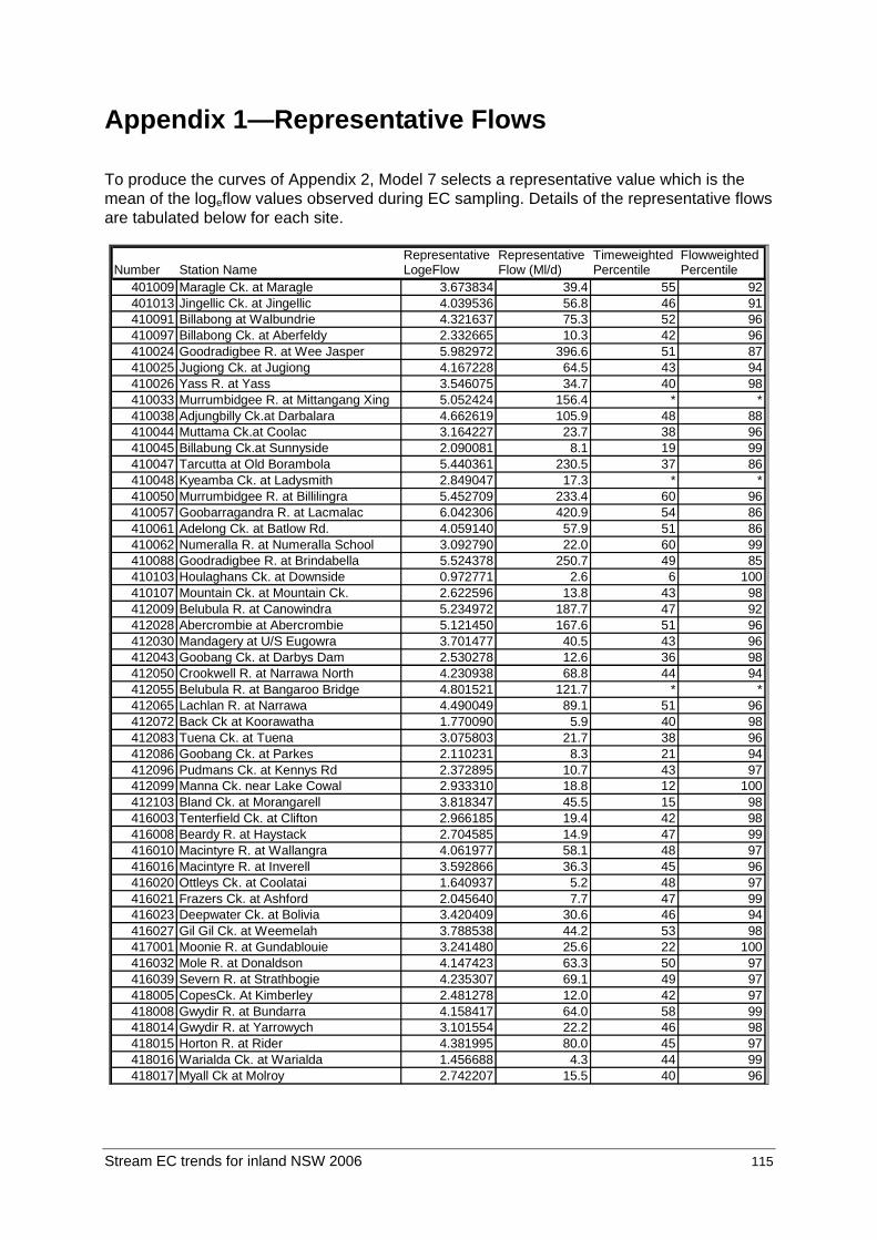
Stream EC trends for inland NSW 2006 115
Appendix 1—Representative Flows
To produce the curves of Appendix 2, Model 7 selects a representative value which is the mean of the logeflow values observed during EC sampling. Details of the representative flows are tabulated below for each site.
Representative Representative Timeweighted FlowweightedNumber Station Name LogeFlow Flow (Ml/d) Percentile Percentile
401009 Maragle Ck. at Maragle 3.673834 39.4 55 92401013 Jingellic Ck. at Jingellic 4.039536 56.8 46 91410091 Billabong at Walbundrie 4.321637 75.3 52 96410097 Billabong Ck. at Aberfeldy 2.332665 10.3 42 96410024 Goodradigbee R. at Wee Jasper 5.982972 396.6 51 87410025 Jugiong Ck. at Jugiong 4.167228 64.5 43 94410026 Yass R. at Yass 3.546075 34.7 40 98410033 Murrumbidgee R. at Mittangang Xing 5.052424 156.4 * *410038 Adjungbilly Ck.at Darbalara 4.662619 105.9 48 88410044 Muttama Ck.at Coolac 3.164227 23.7 38 96410045 Billabung Ck.at Sunnyside 2.090081 8.1 19 99410047 Tarcutta at Old Borambola 5.440361 230.5 37 86410048 Kyeamba Ck. at Ladysmith 2.849047 17.3 * *410050 Murrumbidgee R. at Billilingra 5.452709 233.4 60 96410057 Goobarragandra R. at Lacmalac 6.042306 420.9 54 86410061 Adelong Ck. at Batlow Rd. 4.059140 57.9 51 86410062 Numeralla R. at Numeralla School 3.092790 22.0 60 99410088 Goodradigbee R. at Brindabella 5.524378 250.7 49 85410103 Houlaghans Ck. at Downside 0.972771 2.6 6 100410107 Mountain Ck. at Mountain Ck. 2.622596 13.8 43 98412009 Belubula R. at Canowindra 5.234972 187.7 47 92412028 Abercrombie at Abercrombie 5.121450 167.6 51 96412030 Mandagery at U/S Eugowra 3.701477 40.5 43 96412043 Goobang Ck. at Darbys Dam 2.530278 12.6 36 98412050 Crookwell R. at Narrawa North 4.230938 68.8 44 94412055 Belubula R. at Bangaroo Bridge 4.801521 121.7 * *412065 Lachlan R. at Narrawa 4.490049 89.1 51 96412072 Back Ck at Koorawatha 1.770090 5.9 40 98412083 Tuena Ck. at Tuena 3.075803 21.7 38 96412086 Goobang Ck. at Parkes 2.110231 8.3 21 94412096 Pudmans Ck. at Kennys Rd 2.372895 10.7 43 97412099 Manna Ck. near Lake Cowal 2.933310 18.8 12 100412103 Bland Ck. at Morangarell 3.818347 45.5 15 98416003 Tenterfield Ck. at Clifton 2.966185 19.4 42 98416008 Beardy R. at Haystack 2.704585 14.9 47 99416010 Macintyre R. at Wallangra 4.061977 58.1 48 97416016 Macintyre R. at Inverell 3.592866 36.3 45 96416020 Ottleys Ck. at Coolatai 1.640937 5.2 48 97416021 Frazers Ck. at Ashford 2.045640 7.7 47 99416023 Deepwater Ck. at Bolivia 3.420409 30.6 46 94416027 Gil Gil Ck. at Weemelah 3.788538 44.2 53 98417001 Moonie R. at Gundablouie 3.241480 25.6 22 100416032 Mole R. at Donaldson 4.147423 63.3 50 97416039 Severn R. at Strathbogie 4.235307 69.1 49 97418005 CopesCk. At Kimberley 2.481278 12.0 42 97418008 Gwydir R. at Bundarra 4.158417 64.0 58 99418014 Gwydir R. at Yarrowych 3.101554 22.2 46 98418015 Horton R. at Rider 4.381995 80.0 45 97418016 Warialda Ck. at Warialda 1.456688 4.3 44 99418017 Myall Ck at Molroy 2.742207 15.5 40 96

116 Stream EC trends for inland NSW 2006
Representative Representative Timeweighted FlowweightedNumber Station Name LogeFlow Flow (Ml/d) Percentile Percentile
418018 Keera Ck. at Keera 2.761794 15.8 43 97418021 Laura Ck. at Laura 2.704628 14.9 38 98418023 Moredun Ck. at Bundarra 3.286010 26.7 41 98418025 Halls Ck. at Bingara 2.310812 10.1 30 78418027 Horton R. at DamSite 1.977068 7.2 45 99418029 Gwydir R. at Stoneybatter 4.111625 61.0 52 98418032 Tycannah Ck. at Horseshoe 2.306464 10.0 27 98418052 Carole Ck. Nr. Garah 4.363104 78.5 45 93419005 Namoi R. at Nth Cuerindi 5.100244 164.1 49 95419016 Cockburn R. at Mulla Xing 3.383754 29.5 46 98419027 Mooki R. at Breeza 2.677924 14.6 42 99419029 Halls Ck. At Ukalon 2.746187 15.6 30 92419032 Coxs Ck.at Boggabri 2.887043 17.9 17 100419033 Coxs Ck.at Tambar Springs 1.704663 5.5 52 98419035 Goonoo Ck. at Timbumburi 2.401605 11.0 41 97419051 Maules Ck.at Avoca 2.514995 12.4 * *419053 Manilla R. at Black Springs 3.087662 21.9 44 95419054 Swamp Oak Ck. At Limbri 2.469337 11.8 41 98419072 Baradine Ck.at Kienbri 2.495872 12.1 20 98420003 Belar Ck. at Warkton 1.913105 6.8 37 93420004 Castlereagh R. at Mendooran 3.748378 42.5 38 96420005 Castlereagh R. at Coonamble 5.682852 293.8 18 92420010 Wallumburrawang Ck. at Bearbung 2.271084 9.7 16 98420012 Butheroo Ck. at Neilrex -1.000777 0.4 41 100420015 Warrena Ck. At Warrana 1.083901 3.0 18 100420017 Castlereagh R. at Hidden Valley 2.707426 15.0 44 97421018 Bell R. at Newrea 4.346818 77.2 44 94421023 Bogan R. at Gongolon 4.521186 91.9 41 98421025 Macquarie R. at Bruinbun 5.443971 231.4 52 96421026 Turon R. at Sofala 3.964065 52.7 41 96421035 Fish R. at Tarana 4.749757 115.6 48 90421039 Bogan R. at Neurie Plains 3.723974 41.4 18 99421042 Talbragar R. at Elong Elong 3.386099 29.6 43 98421048 Little R. at Obley 2.802105 16.5 30 97421055 Coolbaggie Ck. at Rawsonville 2.316237 10.1 13 99421056 Coolaburragundy Ck. at Coolah 2.077902 8.0 51 95421059 Buckinbar Ck. at Yeoval 2.624640 13.8 22 56421072 Winburndale Rivulet. at Howards Bridge 4.081947 59.3 44 95421073 Meroo Ck. At Yarrabin 2 3.562517 35.3 10 98421076 Bogan R. at Peak Hill 2 4.023535 55.9 8 97421084 Burrill Ck. At Mickibri 2.214165 9.2 12 97421101 Campbells R. U/S Ben Chifley Dam 3.526172 34.0 58 98

Stream EC trends for inland NSW 2006 117
Appendix 2—Fitted Response Curves
The following 92 graphs illustrate the performance of Models 3 and 7 in fitting the observed data points. The chart on the left uses the data directly from the TRITON archive. The chart on the right uses data adjusted as described in Annexure A.
Generally, the charts on the left are more relevant. As an exception, the datasets of the 3 northern valleys—Border Rivers, Gwydir and Namoi (Appendices 2.34 to 2.69)—have undergone an adjustment in the early years; the charts on the right are thus more relevant.
The green spiked response line represents the fitted values from Model 7, solved at the actual observed values of flow, seasonality and time. How well the model fits these data is illustrated by the extent to which the green line extends towards the observed points.
The blue smoothed curve is obtained from Model 5, and is solved at the mean values of flow and seasonality. It is smooth because it indicates the spline (linear and non-linear) effects of time for an average effect of flow and seasonality.

118 S
tream E
C trends for inland N
SW
2006

Stream
EC
trends for inland NS
W 2006
119

120 S
tream E
C trends for inland N
SW
2006

Stream
EC
trends for inland NS
W 2006
121

122 S
tream E
C trends for inland N
SW
2006
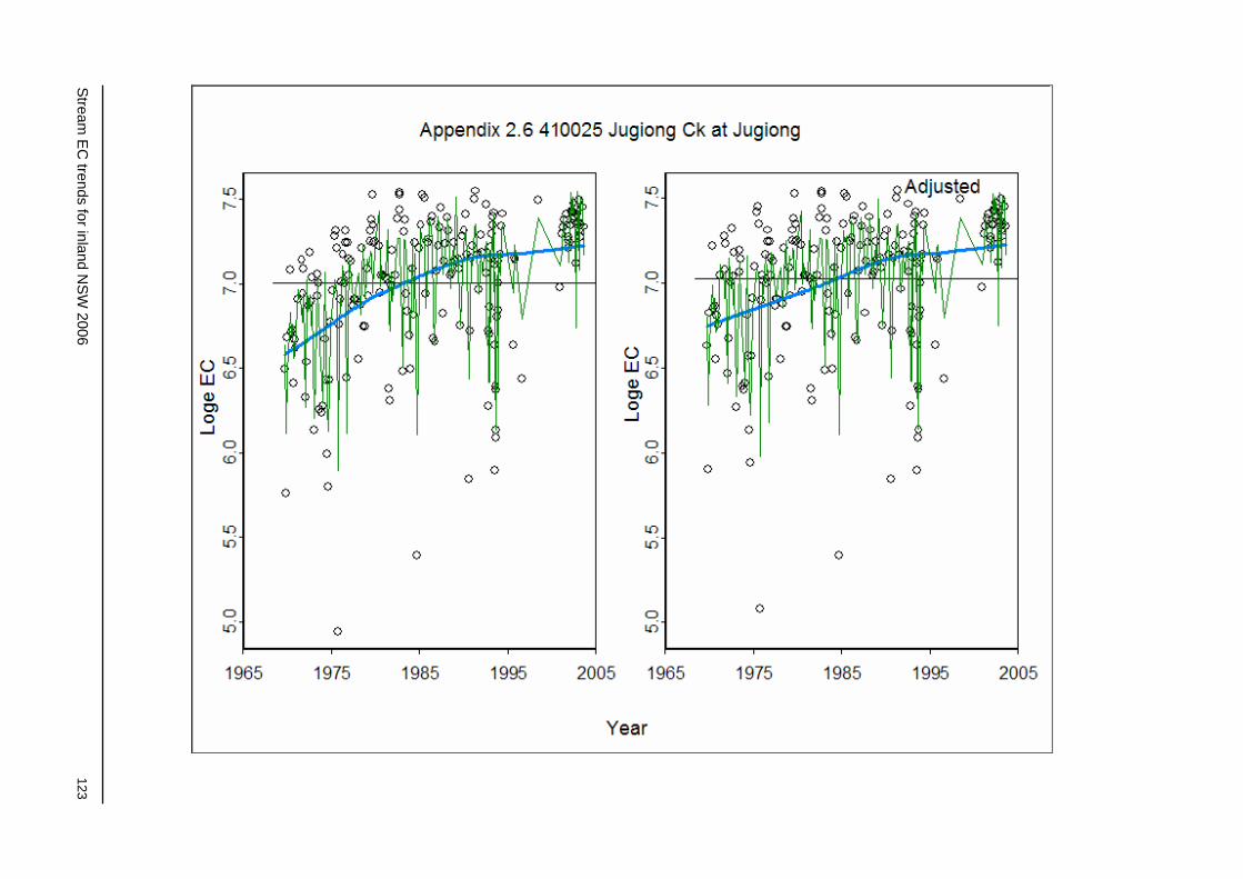
Stream
EC
trends for inland NS
W 2006
123

124 S
tream E
C trends for inland N
SW
2006
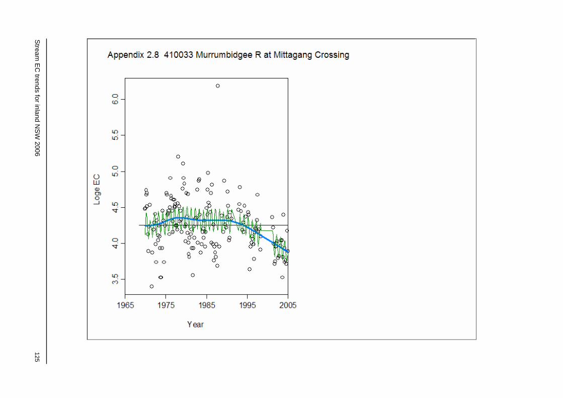
Stream
EC
trends for inland NS
W 2006
125
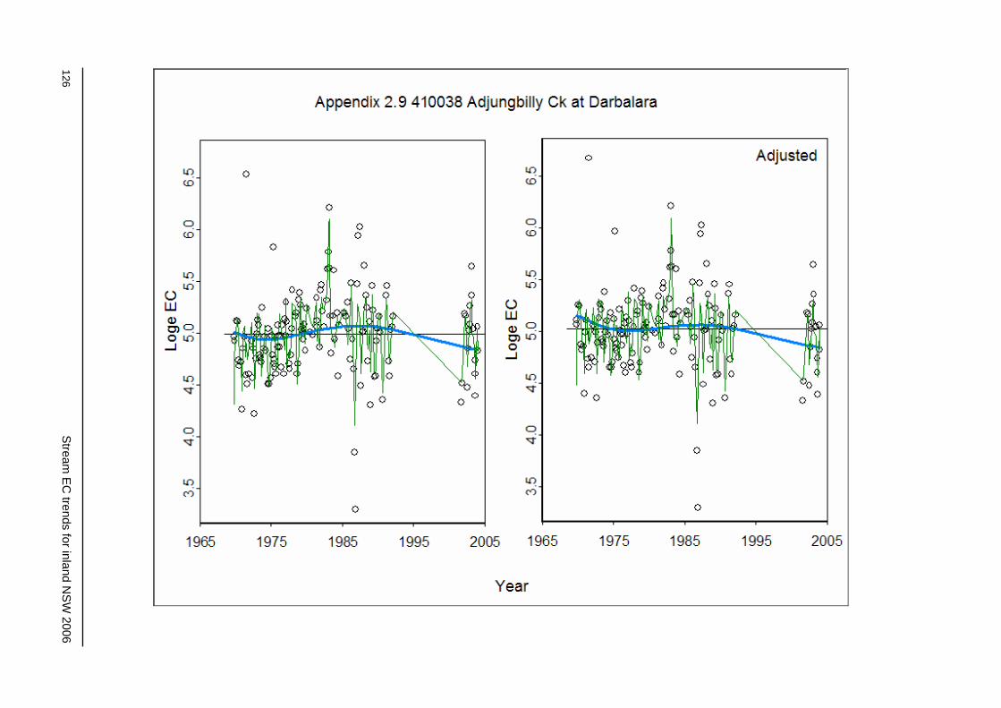
126 S
tream E
C trends for inland N
SW
2006

Stream
EC
trends for inland NS
W 2006
127
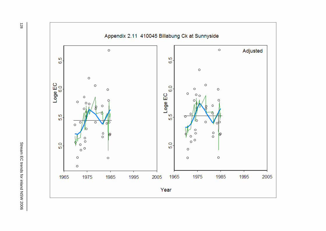
128 S
tream E
C trends for inland N
SW
2006

Stream
EC
trends for inland NS
W 2006
129

130 S
tream E
C trends for inland N
SW
2006

Stream
EC
trends for inland NS
W 2006
131

132 S
tream E
C trends for inland N
SW
2006

Stream
EC
trends for inland NS
W 2006
133
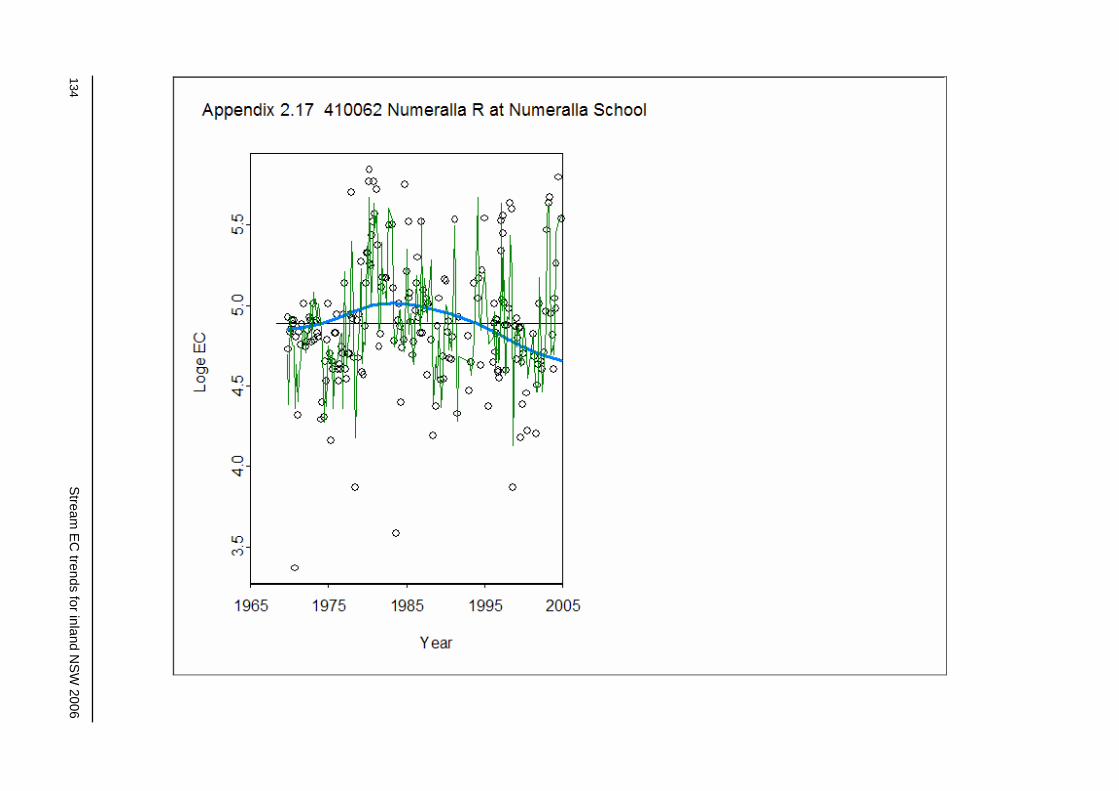
134 S
tream E
C trends for inland N
SW
2006

Stream
EC
trends for inland NS
W 2006
135

136 S
tream E
C trends for inland N
SW
2006

Stream
EC
trends for inland NS
W 2006
137

138 S
tream E
C trends for inland N
SW
2006

Stream
EC
trends for inland NS
W 2006
139

140 S
tream E
C trends for inland N
SW
2006
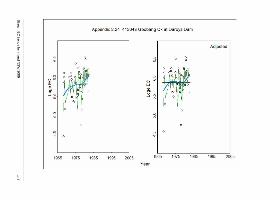
Stream
EC
trends for inland NS
W 2006
141

142 S
tream E
C trends for inland N
SW
2006
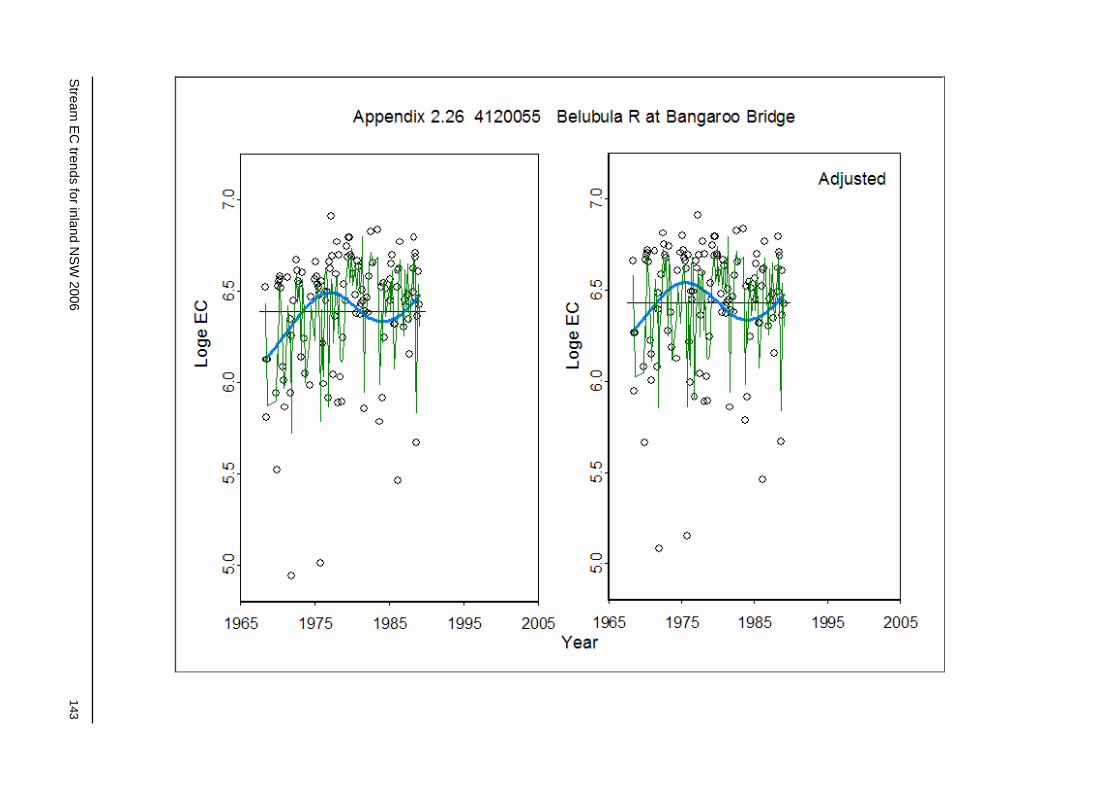
Stream
EC
trends for inland NS
W 2006
143
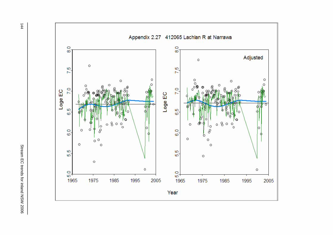
144 S
tream E
C trends for inland N
SW
2006
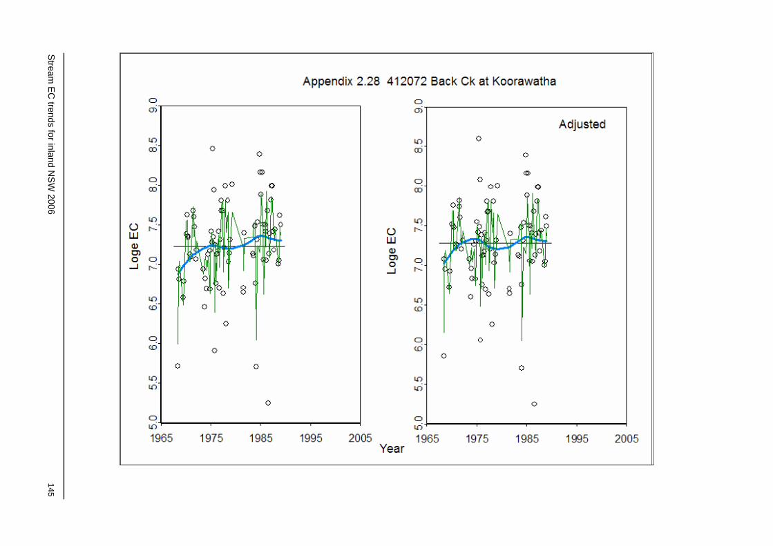
Stream
EC
trends for inland NS
W 2006
145

146 S
tream E
C trends for inland N
SW
2006

Stream
EC
trends for inland NS
W 2006
147

148 S
tream E
C trends for inland N
SW
2006
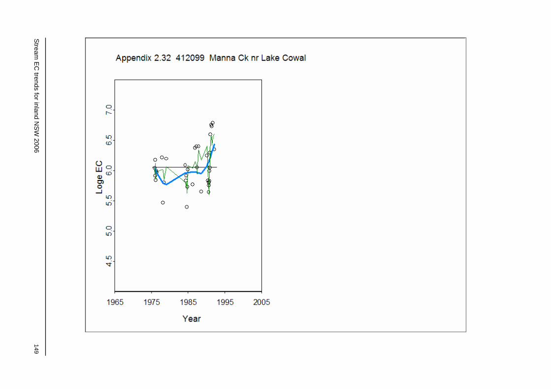
Stream
EC
trends for inland NS
W 2006
149
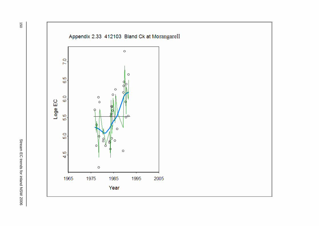
150 S
tream E
C trends for inland N
SW
2006
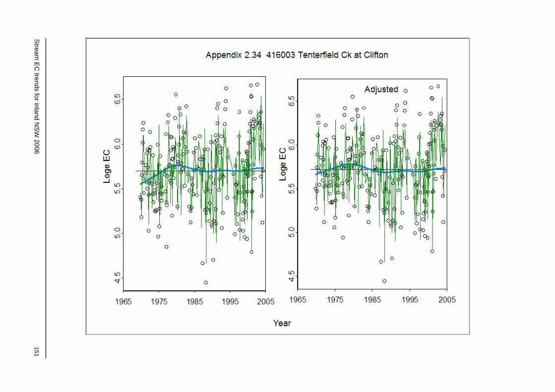
Stream
EC
trends for inland NS
W 2006
151

152 S
tream E
C trends for inland N
SW
2006

Stream
EC
trends for inland NS
W 2006
153

154 S
tream E
C trends for inland N
SW
2006

Stream
EC
trends for inland NS
W 2006
155
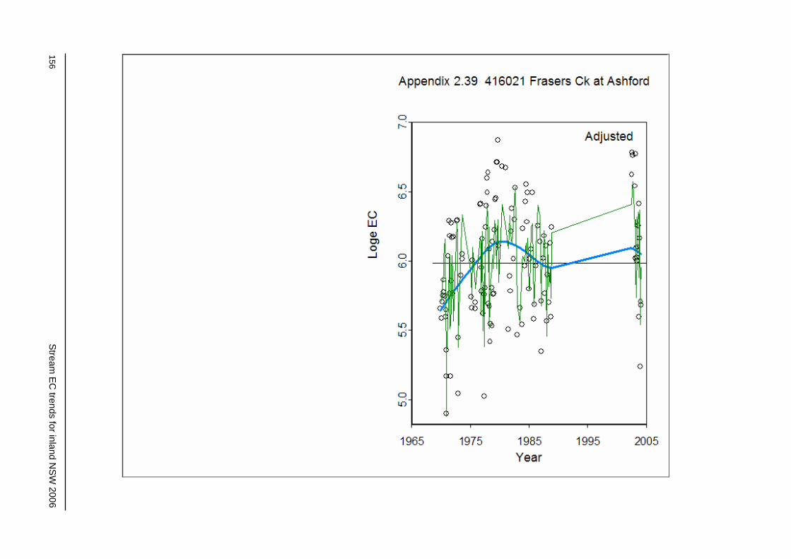
156 S
tream E
C trends for inland N
SW
2006

Stream
EC
trends for inland NS
W 2006
157
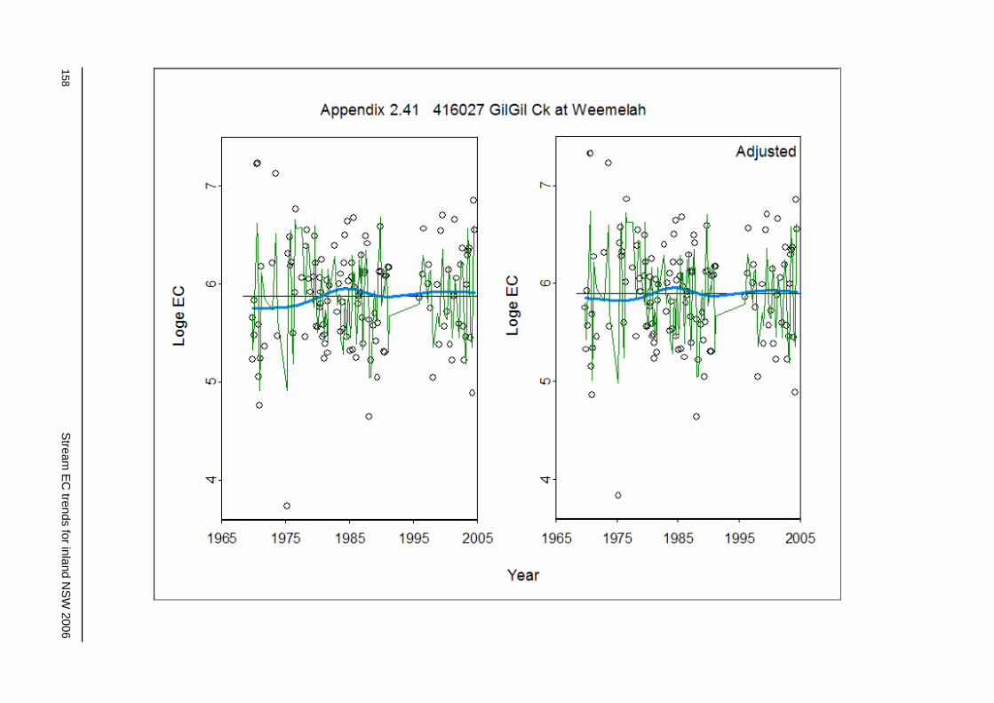
158 S
tream E
C trends for inland N
SW
2006

Stream
EC
trends for inland NS
W 2006
159

160 S
tream E
C trends for inland N
SW
2006
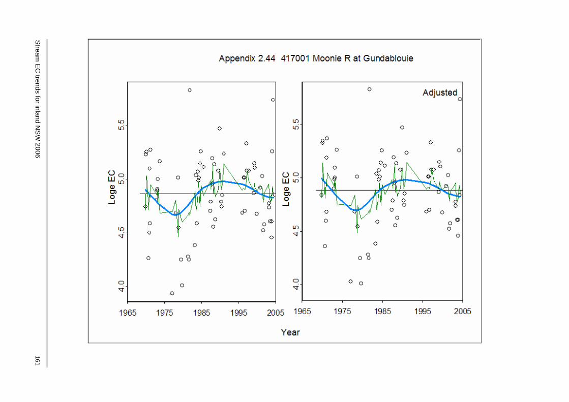
Stream
EC
trends for inland NS
W 2006
161

162 S
tream E
C trends for inland N
SW
2006
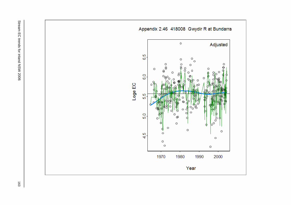
Stream
EC
trends for inland NS
W 2006
163
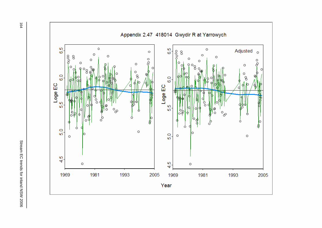
164 S
tream E
C trends for inland N
SW
2006

Stream
EC
trends for inland NS
W 2006
165

166 S
tream E
C trends for inland N
SW
2006

Stream
EC
trends for inland NS
W 2006
167
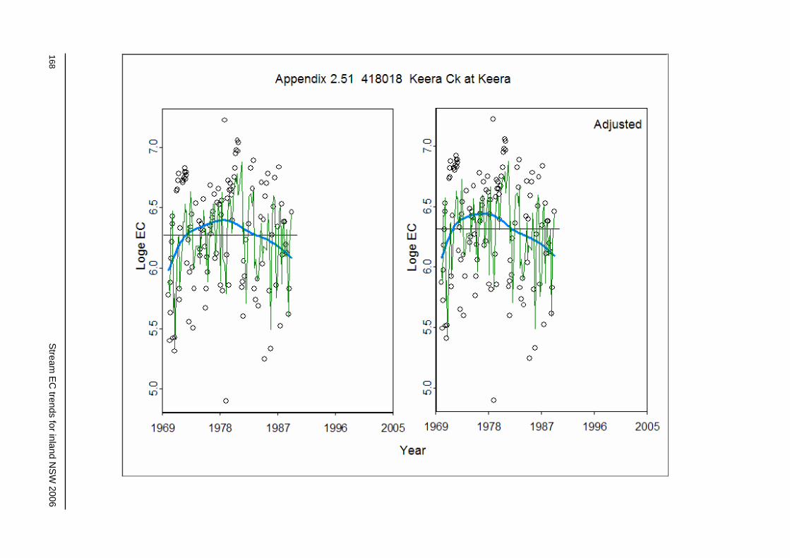
168 S
tream E
C trends for inland N
SW
2006

Stream
EC
trends for inland NS
W 2006
169
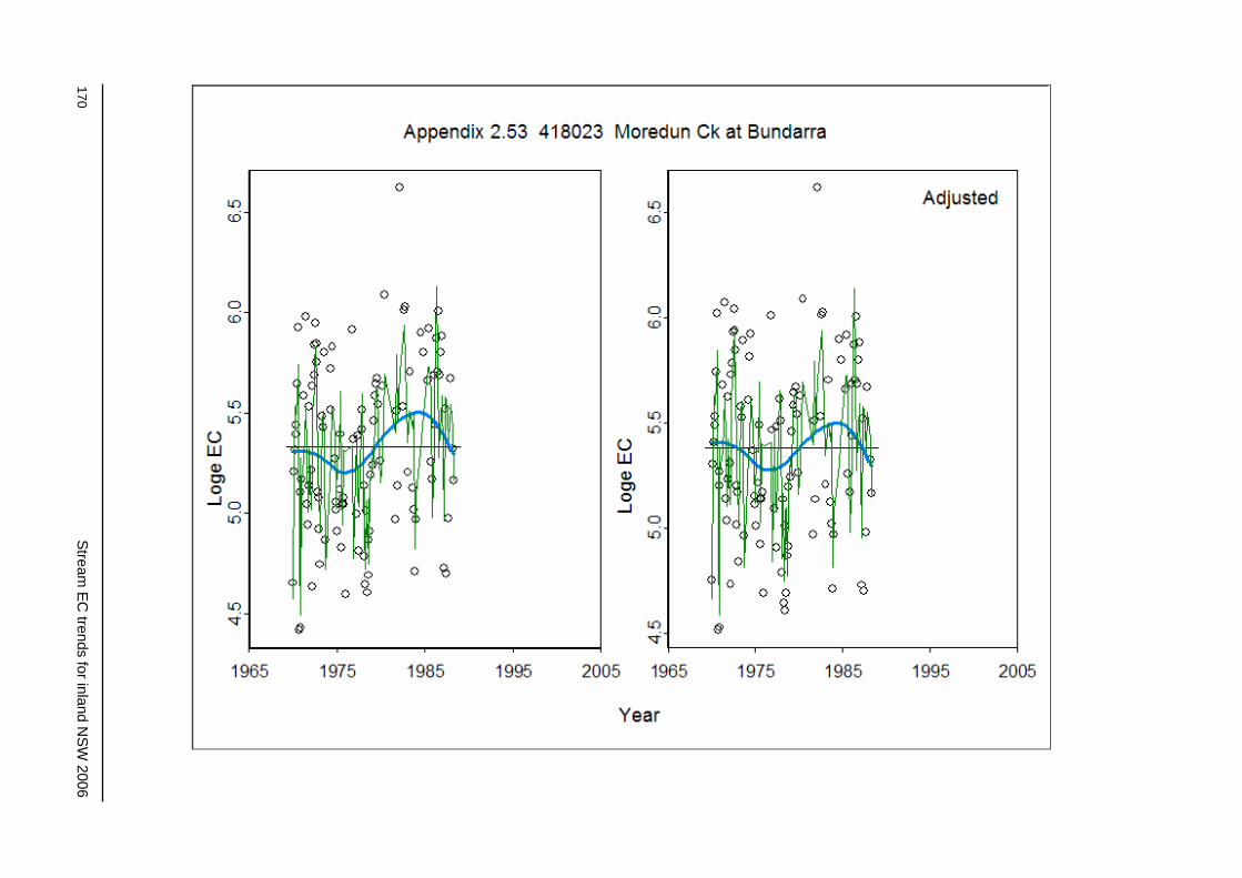
170 S
tream E
C trends for inland N
SW
2006
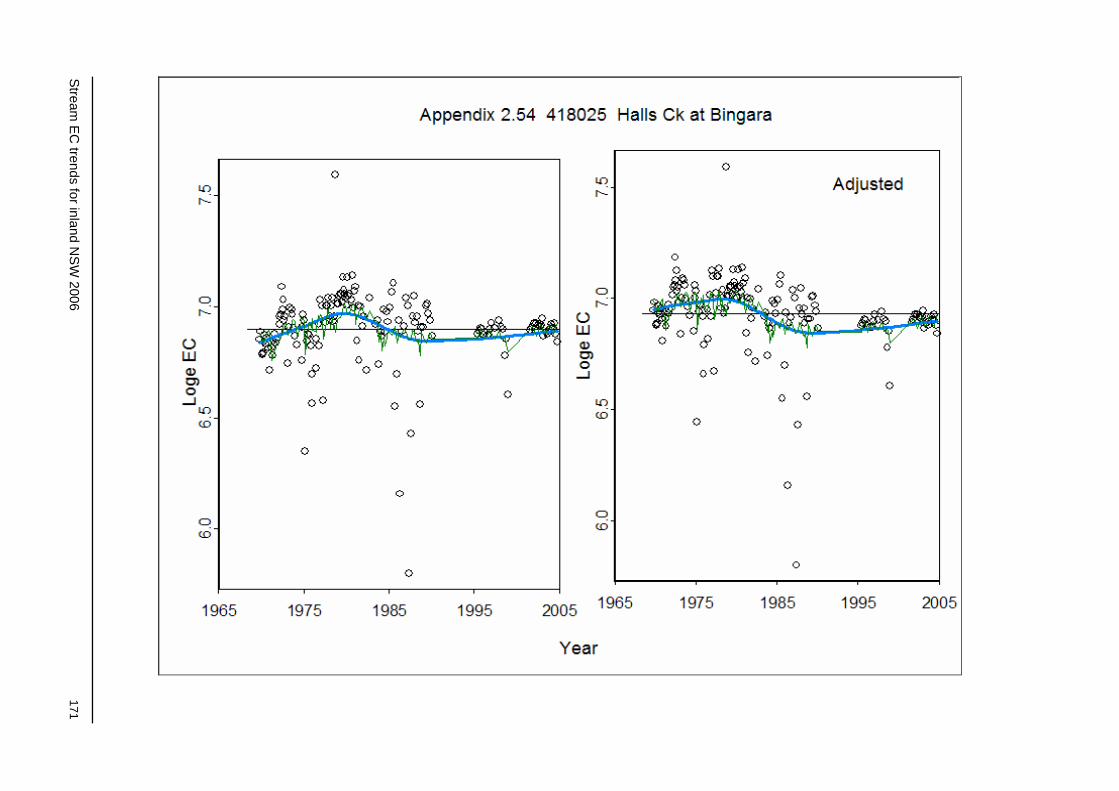
Stream
EC
trends for inland NS
W 2006
171
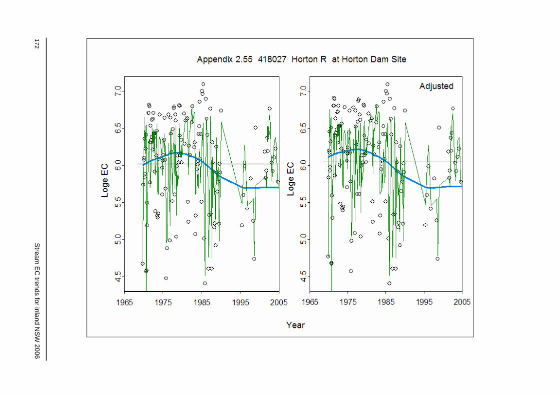
172 S
tream E
C trends for inland N
SW
2006

Stream
EC
trends for inland NS
W 2006
173
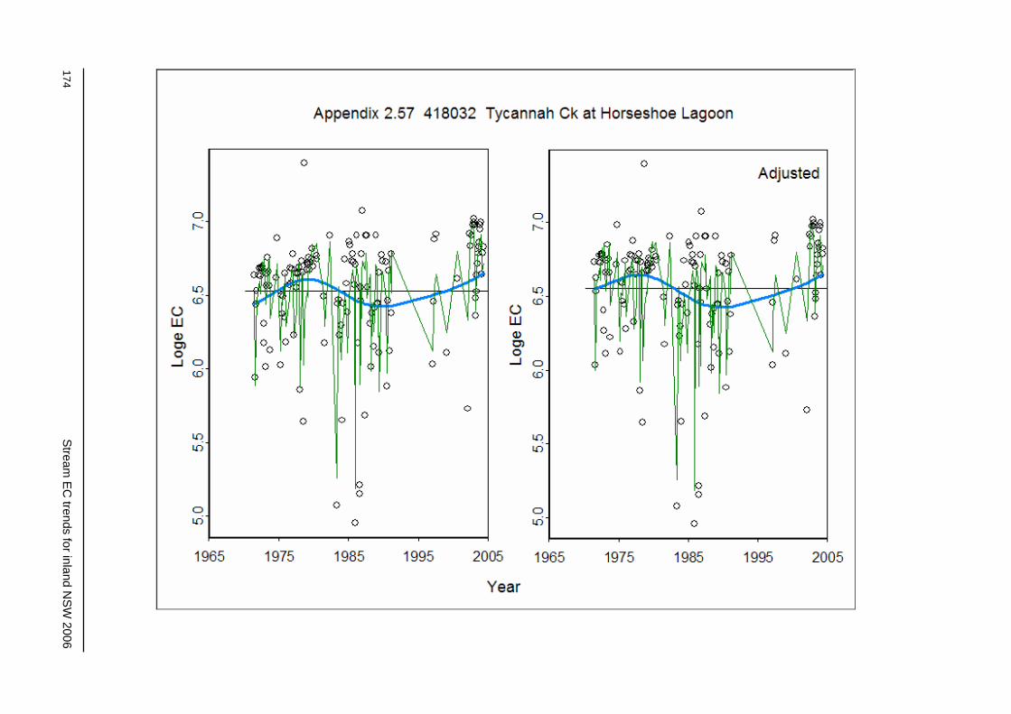
174 S
tream E
C trends for inland N
SW
2006
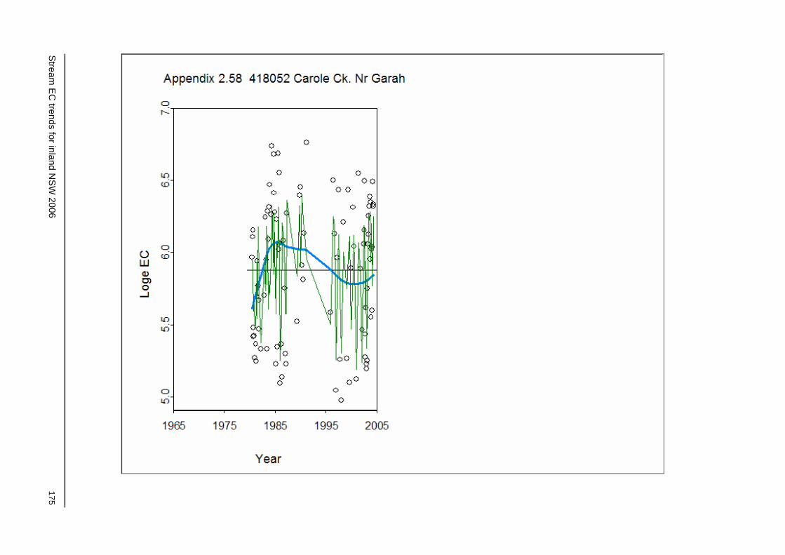
Stream
EC
trends for inland NS
W 2006
175

176 S
tream E
C trends for inland N
SW
2006
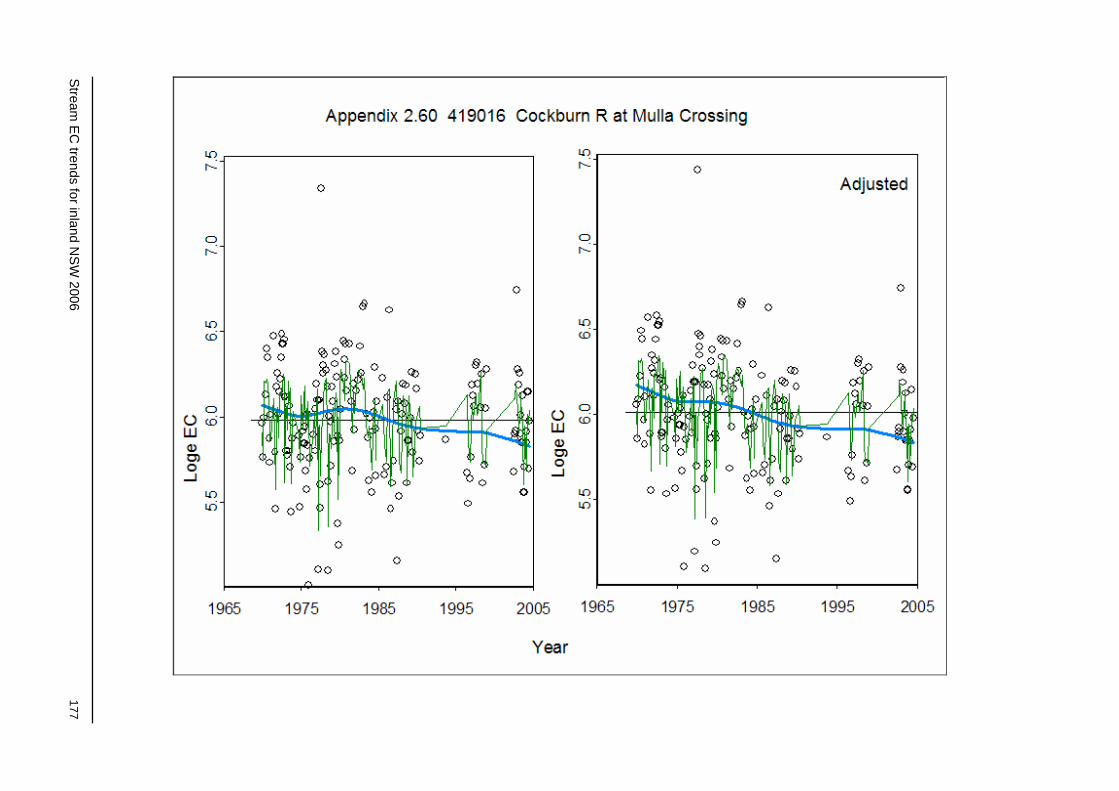
Stream
EC
trends for inland NS
W 2006
177

178 S
tream E
C trends for inland N
SW
2006

Stream
EC
trends for inland NS
W 2006
179

180 S
tream E
C trends for inland N
SW
2006

Stream
EC
trends for inland NS
W 2006
181

182 S
tream E
C trends for inland N
SW
2006

Stream
EC
trends for inland NS
W 2006
183
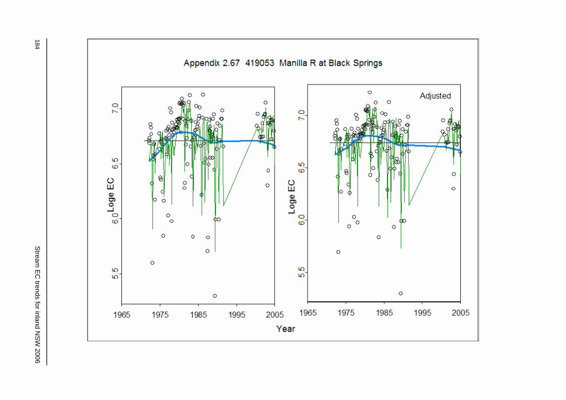
184 S
tream E
C trends for inland N
SW
2006

Stream
EC
trends for inland NS
W 2006
185
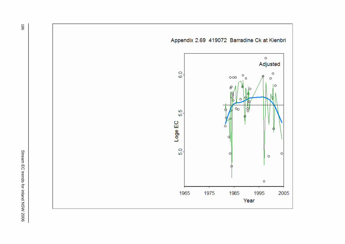
186 S
tream E
C trends for inland N
SW
2006

Stream
EC
trends for inland NS
W 2006
187
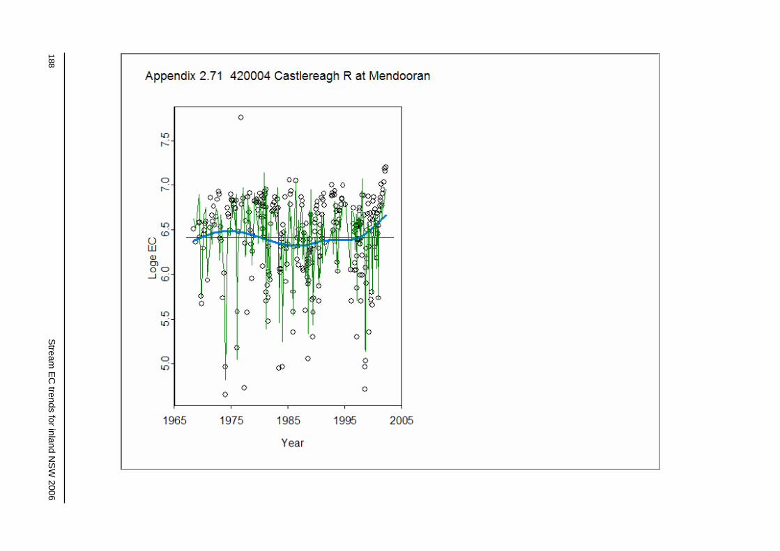
188 S
tream E
C trends for inland N
SW
2006

Stream
EC
trends for inland NS
W 2006
189
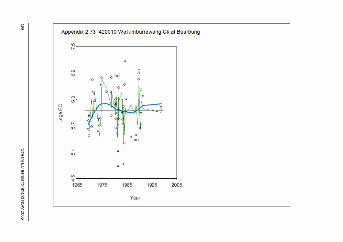
190 S
tream E
C trends for inland N
SW
2006

Stream
EC
trends for inland NS
W 2006
191

192 S
tream E
C trends for inland N
SW
2006

Stream
EC
trends for inland NS
W 2006
193
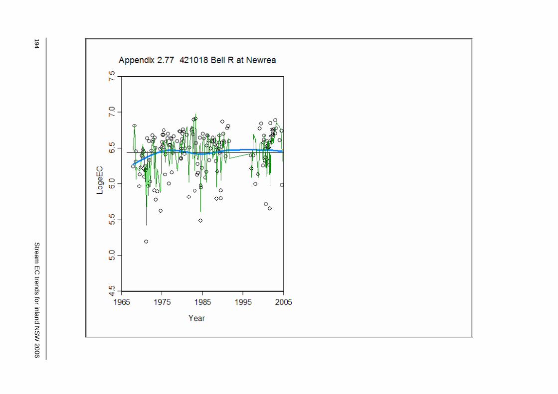
194 S
tream E
C trends for inland N
SW
2006

Stream
EC
trends for inland NS
W 2006
195

196 S
tream E
C trends for inland N
SW
2006

Stream
EC
trends for inland NS
W 2006
197

198 S
tream E
C trends for inland N
SW
2006

Stream
EC
trends for inland NS
W 2006
199
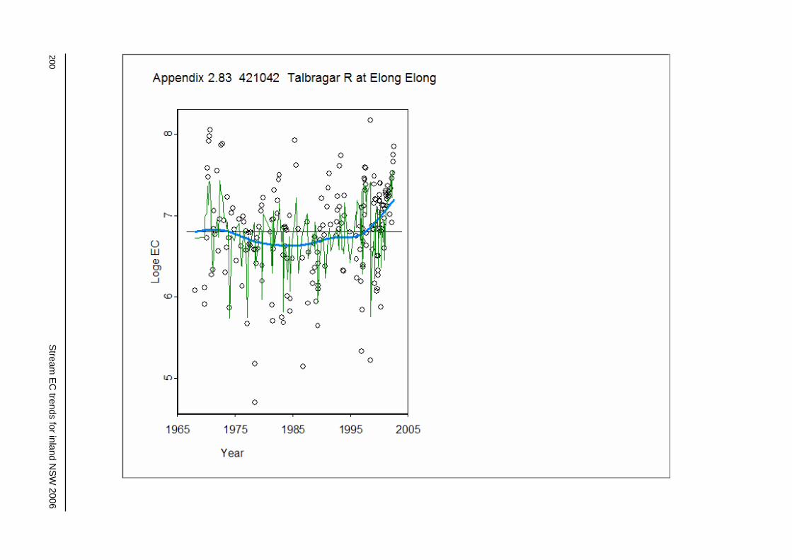
200 S
tream E
C trends for inland N
SW
2006

Stream
EC
trends for inland NS
W 2006
201
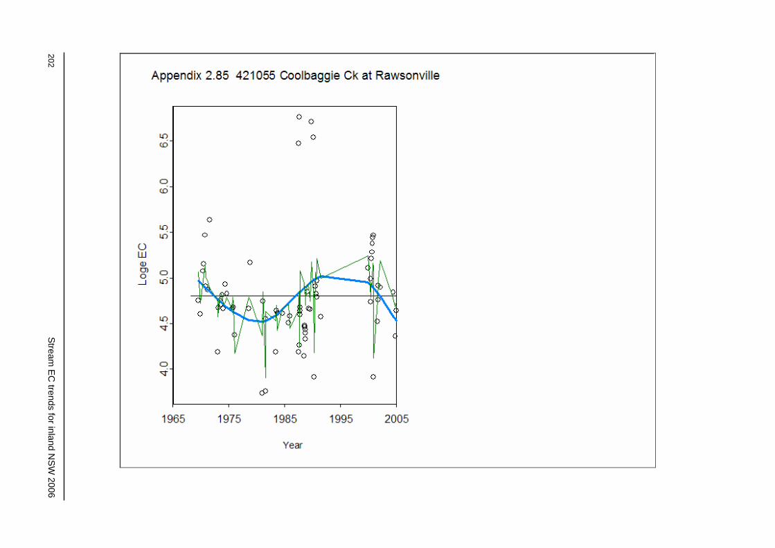
202 S
tream E
C trends for inland N
SW
2006

Stream
EC
trends for inland NS
W 2006
203

204 S
tream E
C trends for inland N
SW
2006

Stream
EC
trends for inland NS
W 2006
205

206 S
tream E
C trends for inland N
SW
2006

Stream
EC
trends for inland NS
W 2006
207

208 S
tream E
C trends for inland N
SW
2006

Stream
EC
trends for inland NS
W 2006
209

210 S
tream E
C trends for inland N
SW
2006
Appendix 3—Base Flow Separation
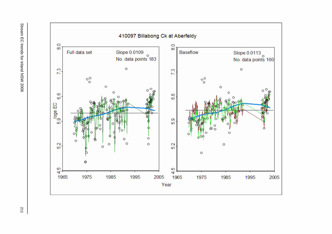
Stream
EC
trends for inland NS
W 2006
211

212 S
tream E
C trends for inland N
SW
2006
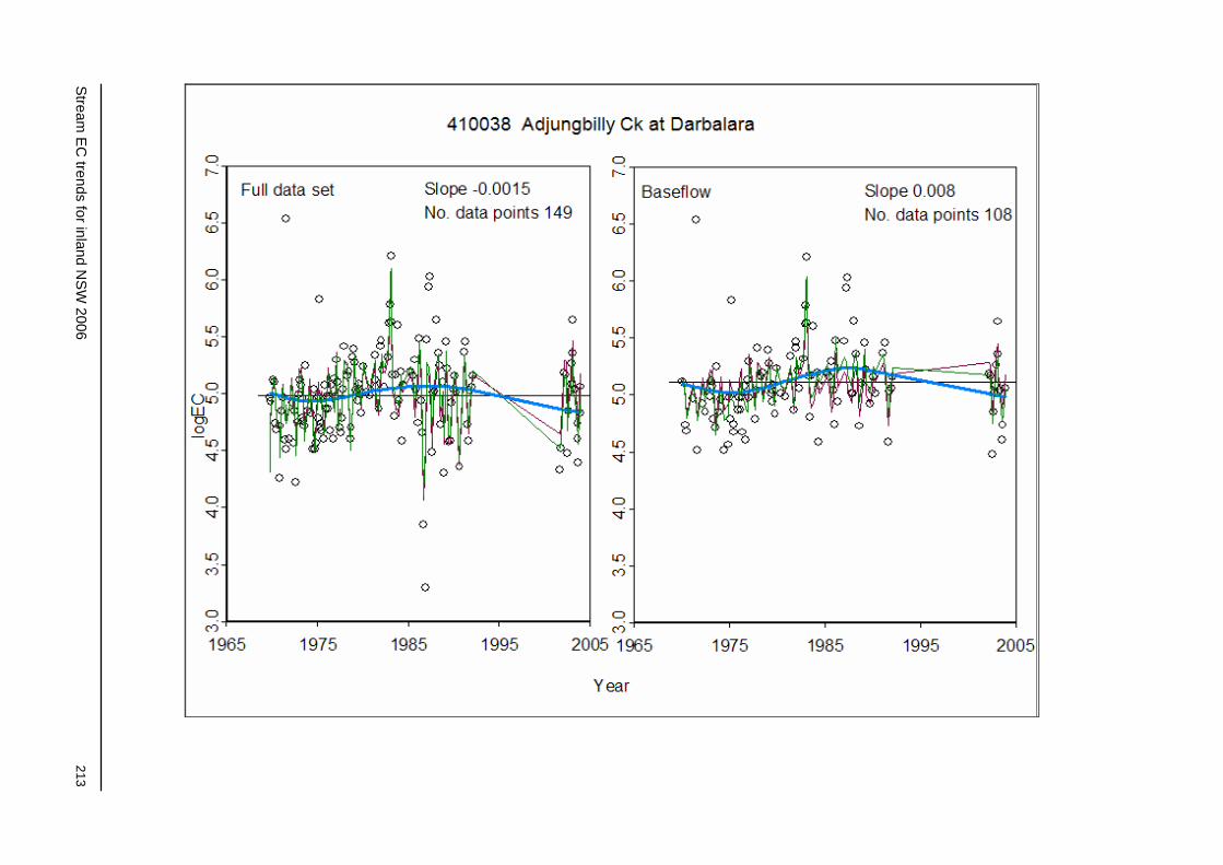
Stream
EC
trends for inland NS
W 2006
213

214 S
tream E
C trends for inland N
SW
2006

Stream
EC
trends for inland NS
W 2006
215

216 S
tream E
C trends for inland N
SW
2006

Stream
EC
trends for inland NS
W 2006
217

218 S
tream E
C trends for inland N
SW
2006
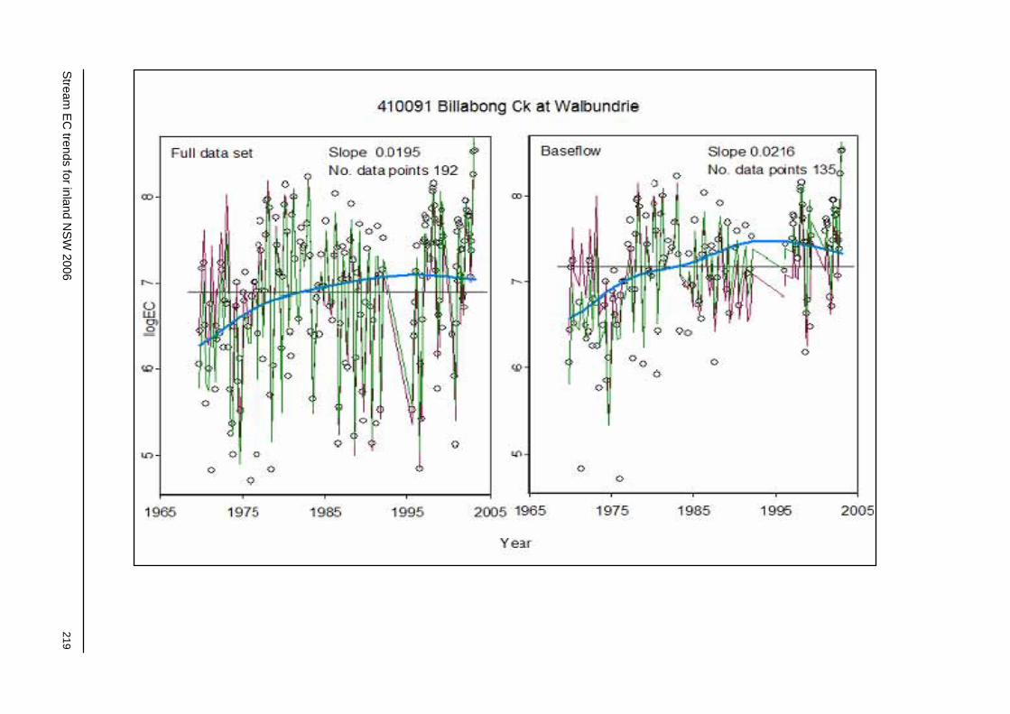
Stream
EC
trends for inland NS
W 2006
219
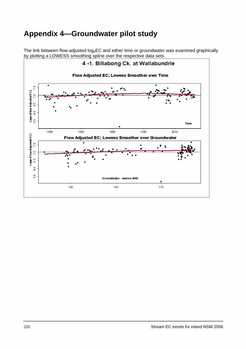
220 Stream EC trends for inland NSW 2006
Appendix 4—Groundwater pilot study
The link between flow-adjusted logeEC and either time or groundwater was examined graphically by plotting a LOWESS smoothing spline over the respective data sets.
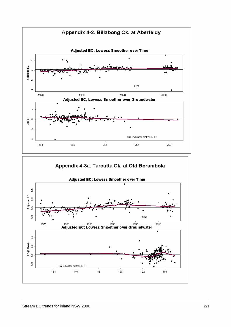
Stream EC trends for inland NSW 2006 221

222 Stream EC trends for inland NSW 2006

Stream EC trends for inland NSW 2006 223

224 Stream EC trends for inland NSW 2006
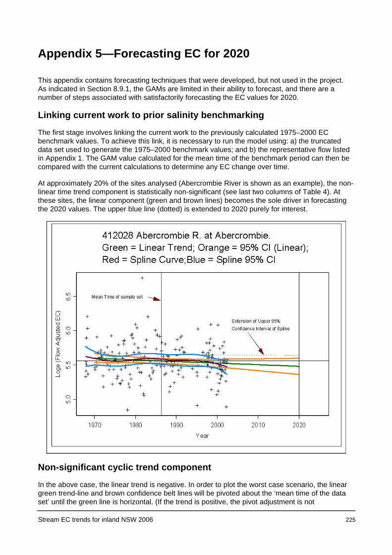
Stream EC trends for inland NSW 2006 225
Appendix 5—Forecasting EC for 2020
This appendix contains forecasting techniques that were developed, but not used in the project. As indicated in Section 8.9.1, the GAMs are limited in their ability to forecast, and there are a number of steps associated with satisfactorily forecasting the EC values for 2020.
Linking current work to prior salinity benchmarking
The first stage involves linking the current work to the previously calculated 1975–2000 EC benchmark values. To achieve this link, it is necessary to run the model using: a) the truncated data set used to generate the 1975–2000 benchmark values; and b) the representative flow listed in Appendix 1. The GAM value calculated for the mean time of the benchmark period can then be compared with the current calculations to determine any EC change over time.
At approximately 20% of the sites analysed (Abercrombie River is shown as an example), the non-linear time trend component is statistically non-significant (see last two columns of Table 4). At these sites, the linear component (green and brown lines) becomes the sole driver in forecasting the 2020 values. The upper blue line (dotted) is extended to 2020 purely for interest.
Non-significant cyclic trend component
In the above case, the linear trend is negative. In order to plot the worst case scenario, the linear green trend-line and brown confidence belt lines will be pivoted about the ‘mean time of the data set’ until the green line is horizontal. (If the trend is positive, the pivot adjustment is not
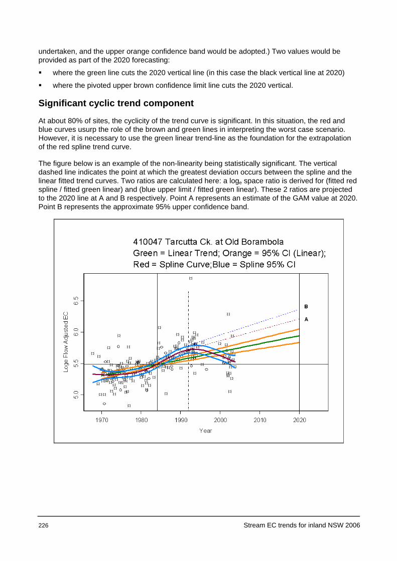
226 Stream EC trends for inland NSW 2006
undertaken, and the upper orange confidence band would be adopted.) Two values would be provided as part of the 2020 forecasting:
where the green line cuts the 2020 vertical line (in this case the black vertical line at 2020)
where the pivoted upper brown confidence limit line cuts the 2020 vertical.
Significant cyclic trend component
At about 80% of sites, the cyclicity of the trend curve is significant. In this situation, the red and blue curves usurp the role of the brown and green lines in interpreting the worst case scenario. However, it is necessary to use the green linear trend-line as the foundation for the extrapolation of the red spline trend curve.
The figure below is an example of the non-linearity being statistically significant. The vertical dashed line indicates the point at which the greatest deviation occurs between the spline and the linear fitted trend curves. Two ratios are calculated here: a loge space ratio is derived for (fitted red spline / fitted green linear) and (blue upper limit / fitted green linear). These 2 ratios are projected to the 2020 line at A and B respectively. Point A represents an estimate of the GAM value at 2020. Point B represents the approximate 95% upper confidence band.

Stream EC trends for inland NSW 2006 227
Appendix 6 – S-PLUS Script Input File
# ######################################################################################
# These are the models being fitted in this program
#
# 1. Data.lm1 <- lm(logEC ~ logFlow )
# 2. Data.lm2 <- lm(logEC ~ logFlow + cost + sint)
# 3. Data.gam1 <- gam(logEC ~ s(logFlow,2) + cost + sint)
# 3a D.gam1a <- gam(logEC ~ s(logFlow,2) + cost + sint + s(groundwater,2))
# 4. Data.lm3 <- lm(AdjEC ~ yrfrac)
# 5. Data.gam2 <- gam(AdjEC ~ s(yrfrac, 4))
# 6. Data.lm4 <- lm(logEC ~ logFlow + cost + sint + yrfrac)
# 7. Data.gam3 <- gam(logEC ~ s(logFlow,2) + cost + sint + s(yrfrac, 4))
# 7a D.gam3a <- gam(logEC ~ s(logFlow,2) + cost + sint + s(groundwater, 4)) + s(yrfrac,2)
# ######################################################################################
# =1=1=1=1=1=1=1=1=1=1=1=1=1=1=1=1=1=1=1=1=1=1=1=1=1=1=1=1=1=1=1=1=1=1=1=1=1=1=1=1
# ============== Create a "Data" data frame to save having to rename everything ==
# ================================================================================
Data <- wallallgw # use a common data frame name of Data
attach(Data) # attach desired data frame
dim(Data)
Data[1:3,]
mon <- months(Data$dtime) # generate vector of months
yday <- yeardays(Data$dtime) # generate vector of days from start of year
cost <- cos((2 * pi * yday/365)) # dummy variables for season
sint <- sin((2 * pi * yday/365))
yrfrac <- as.numeric(as.character(years(Data$dtime))) + yday/365
Data$yrfrac <- yrfrac
# =2=2=2=2=2=2=2=2=2=2=2=2=2=2=2=2=2=2=2=2=2=2=2=2=2=2=2=2=2=2=2=2=2=2=2=2=
# ============== How regular are the sampling intervals?===================
# =========================================================================
mon
diff(yrfrac)*365 # number of days lapsed between observations
table(years(dtime), mon) # number of observations per month & year
table(years(dtime)) # how many observations per year ?
# =3=3=3=3=3=3=3=3=3=3=3=3=3=3=3=3=3=3=3=3=3=3=3=3=3=3=3=3=3=3=3=3=3=3=3=3=
# ============== EDA to look for possible seasonality =====================
# =========================================================================
par(mfrow=c(2,2))
logEC <- log(TumutEC)
Data$logEC <- log(TumutEC)
min(instFlow)
logFlow <- log(instFlow)
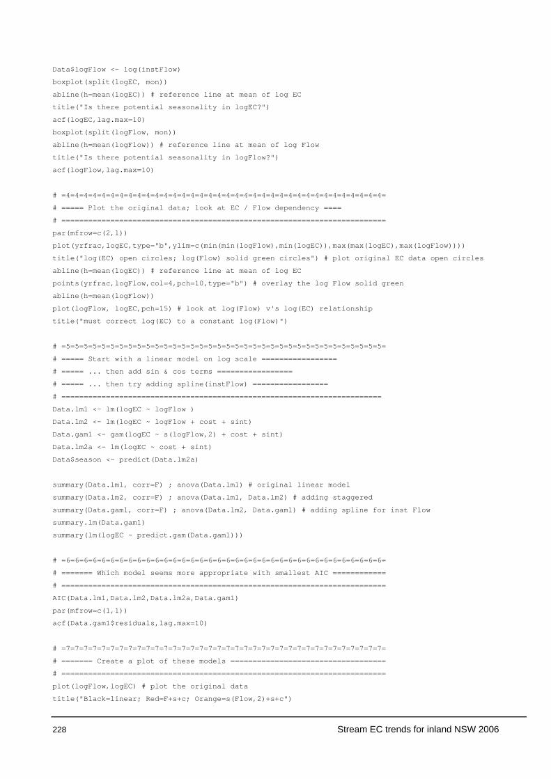
228 Stream EC trends for inland NSW 2006
Data$logFlow <- log(instFlow)
boxplot(split(logEC, mon))
abline(h=mean(logEC)) # reference line at mean of log EC
title("Is there potential seasonality in logEC?")
acf(logEC,lag.max=10)
boxplot(split(logFlow, mon))
abline(h=mean(logFlow)) # reference line at mean of log Flow
title("Is there potential seasonality in logFlow?")
acf(logFlow,lag.max=10)
# =4=4=4=4=4=4=4=4=4=4=4=4=4=4=4=4=4=4=4=4=4=4=4=4=4=4=4=4=4=4=4=4=4=4=4=4=
# ===== Plot the original data; look at EC / Flow dependency ====
# =========================================================================
par(mfrow=c(2,1))
plot(yrfrac,logEC,type="b",ylim=c(min(min(logFlow),min(logEC)),max(max(logEC),max(logFlow))))
title("log(EC) open circles; log(Flow) solid green circles") # plot original EC data open circles
abline(h=mean(logEC)) # reference line at mean of log EC
points(yrfrac,logFlow,col=4,pch=10,type="b") # overlay the log Flow solid green
abline(h=mean(logFlow))
plot(logFlow, logEC,pch=15) # look at log(Flow) v's log(EC) relationship
title("must correct log(EC) to a constant log(Flow)")
# =5=5=5=5=5=5=5=5=5=5=5=5=5=5=5=5=5=5=5=5=5=5=5=5=5=5=5=5=5=5=5=5=5=5=5=5=
# ===== Start with a linear model on log scale =================
# ===== ... then add sin & cos terms =================
# ===== ... then try adding spline(instFlow) =================
# ========================================================================
Data.lm1 <- lm(logEC ~ logFlow )
Data.lm2 <- lm(logEC ~ logFlow + cost + sint)
Data.gam1 <- gam(logEC ~ s(logFlow,2) + cost + sint)
Data.lm2a <- lm(logEC ~ cost + sint)
Data$season <- predict(Data.lm2a)
summary(Data.lm1, corr=F) ; anova(Data.lm1) # original linear model
summary(Data.lm2, corr=F) ; anova(Data.lm1, Data.lm2) # adding staggered
summary(Data.gam1, corr=F) ; anova(Data.lm2, Data.gam1) # adding spline for inst Flow
summary.lm(Data.gam1)
summary(lm(logEC ~ predict.gam(Data.gam1)))
# =6=6=6=6=6=6=6=6=6=6=6=6=6=6=6=6=6=6=6=6=6=6=6=6=6=6=6=6=6=6=6=6=6=6=6=6=
# ======= Which model seems more appropriate with smallest AIC ============
# =========================================================================
AIC(Data.lm1,Data.lm2,Data.lm2a,Data.gam1)
par(mfrow=c(1,1))
acf(Data.gam1$residuals,lag.max=10)
# =7=7=7=7=7=7=7=7=7=7=7=7=7=7=7=7=7=7=7=7=7=7=7=7=7=7=7=7=7=7=7=7=7=7=7=7=
# ======= Create a plot of these models ===================================
# =========================================================================
plot(logFlow,logEC) # plot the original data
title("Black=linear; Red=F+s+c; Orange=s(Flow,2)+s+c")

Stream EC trends for inland NSW 2006 229
abline(Data.lm2,col=3,lwd=4) # red line is Flow + sin + cos
# create data frame for prediction
dummy <- data.frame(cost = rep(mean(cost), length(cost)))
dummy$sint <- rep(mean(sint), length(sint))
dummy$logFlow <- logFlow
dummy$gam1 <- predict.gam(Data.gam1,dummy,type="response")
points(logFlow, dummy$gam1 , col=5,lwd=4) # orange points are smoothed Flow
# =8=8=8=8=8=8=8=8=8=8=8=8=8=8=8=8=8=8=8=8=8=8=8=8=8=8=8=8=8=8=8=8=8=8=8=8=
# ===== Look at adjusted EC versus time, adjusted for Flow & Seasonality===
# ========================================================================
par(mfrow=c(2,1))
AdjEC <- mean(logEC)+Data.gam1$residuals
Data$AdjEC = AdjEC
#plot(yrfrac,logEC)
plot(yrfrac,AdjEC,pch=16) # now plot EC adjusted for Flow & Seasonality
abline(h=mean(logEC)) # add reference line at mean of log EC
lines(lowess(yrfrac,AdjEC),col=3,lwd=4) # show a lowess smoother over time
title("EC adjusted for Flow & Seasonality; lowess smoother over time")
plot(groundwater,AdjEC,pch=16) # now plot EC adjusted for Flow & Seasonality
abline(h=mean(logEC)) # add reference line at mean of log EC
lines(lowess(groundwater,AdjEC),col=3,lwd=4) # show a lowess smoother over time
title("EC adjusted for Flow & Seasonality; lowess smoother over groundwater")
# =9=9=9=9=9=9=9=9=9=9=9=9=9=9=9=9=9=9=9=9=9=9=9=9=9=9=9=9=9=9=9=9=9=9=9=9=
# ===== Fit Generalized Additive Model to adjusted EC data over time ======
# ===== and plot the linear and {linear + smooth} spline components =======
# =========================================================================
Data.lm3 <- lm(AdjEC ~ yrfrac)
Data.gam2 <- gam(AdjEC ~ s(yrfrac,4))
# Following line added by FJH
Data$Data.gam2 <- predict.gam(Data.gam2) #addition FJH 4th June
summary(Data.lm3); summary(Data.gam2); summary.lm(Data.gam2)
#plot(Data.gam2, se=T)
#abline(h=0) # add reference line at zero
#title("aberall -Zero is the mean (Flow adjusted EC)")
plot(yrfrac,AdjEC) # Plot EC adjusted for Flow & Seasonality
abline(h=mean(logEC)) # add reference line at mean of log EC
lines(yrfrac, predict(Data.lm3), col=4,lwd=4) # show the linear part in green
lines(yrfrac, predict.gam(Data.gam2) , col=5,lwd=4) # add the GAM fitted model in orange
title("Adjusted EC data: Green is linear fit; Orange is spline")
#acf(Data.gam2$residuals,lag.max=10) # check for autocorrelation in residuals
D.lm3a <- lm(AdjEC ~ groundwater)
D.gam2a <- gam(AdjEC ~ s(groundwater,2))
summary(D.lm3a); summary(D.gam2a); summary.lm(D.gam2a)
#plot(D.gam2a, se=T)
#abline(h=0) # add reference line at zero
#title("Zero is the mean (Flow adjusted EC)")
plot(groundwater,AdjEC) # Plot EC adjusted for Flow & Seasonality

230 Stream EC trends for inland NSW 2006
abline(h=mean(logEC)) # add reference line at mean of log EC
wallallgw$AdjEC <- AdjEC
wallallgw$lm3a <- predict(D.lm3a)
wallallgw$gam2a <- predict.gam(D.gam2a)
lines(groundwater, predict(D.lm3a), col=4,lwd=4) # show the linear part in green
lines(groundwater, predict.gam(D.gam2a) , col=5,lwd=4) # add the GAM fitted model in orange
title("Adjusted EC data: Green is linear fit; Orange is spline 2")
#acf(D.gam2a$residuals,lag.max=10) # check for autocorrelation in residuals
AIC(Data.lm1,Data.lm2,Data.lm2a,Data.gam1,Data.lm3,D.lm3a,Data.gam2,D.gam2a)
# =========================================================================
# ===== display the effect of different degrees of smoothing =======
# =========================================================================
fit <- smooth.spline(yrfrac,AdjEC)
fit
Data.gam2 <- gam(AdjEC ~ s(yrfrac, 4))
Data.gam22 <- gam(AdjEC ~ s(yrfrac, 2))
Data.gam26 <- gam(AdjEC ~ s(yrfrac, 6))
Data.gam210 <- gam(AdjEC ~ s(yrfrac, 10))
par(mfrow=c(2,2))
plot(yrfrac,AdjEC, xlab="Year") # Plot EC adjusted for Flow & Seasonality
abline(h=mean(logEC)) # add reference line at mean of log EC
lines(yrfrac, predict(Data.lm3), col=4,lwd=4) # show the linear part in green
lines(yrfrac, predict.gam(Data.gam22) , col=5,lwd=4) # add the GAM fitted model in orange
title("Adjusted EC data: Degree of smoothing = 2")
plot(yrfrac,AdjEC, xlab="Year") # Plot EC adjusted for Flow & Seasonality
abline(h=mean(logEC)) # add reference line at mean of log EC
lines(yrfrac, predict(Data.lm3), col=4,lwd=4) # show the linear part in green
lines(yrfrac, predict.gam(Data.gam2) , col=5,lwd=4) # add the GAM fitted model in orange
title("Adjusted EC data: Degree of smoothing = 4")
plot(yrfrac,AdjEC, xlab="Year") # Plot EC adjusted for Flow & Seasonality
abline(h=mean(logEC)) # add reference line at mean of log EC
lines(yrfrac, predict(Data.lm3), col=4,lwd=4) # show the linear part in green
lines(yrfrac, predict.gam(Data.gam26) , col=5,lwd=4) # add the GAM fitted model in orange
title("Adjusted EC data: Degree of smoothing = 6")
plot(yrfrac,AdjEC, xlab="Year") # Plot EC adjusted for Flow & Seasonality
abline(h=mean(logEC)) # add reference line at mean of log EC
lines(yrfrac, predict(Data.lm3), col=4,lwd=4) # show the linear part in green
lines(yrfrac, predict.gam(Data.gam210) , col=5,lwd=4) # add the GAM fitted model in orange
title("Adjusted EC data: Degree of smoothing = 10")
# 10=10=10=10=10=10=10=10=10=10=10=10=10=10=10=10=10=10=10=10=10=10=10=10=10
# ===== Predict log EC for the first day of each year =====================
# =========================================================================
years <- 2003 - 1970 + 2
yr.margin <- data.frame(yrfrac=seq(from=1970, to=2004, length=years))

Stream EC trends for inland NSW 2006 231
yr.margin$yrfrac[35] <- mean(yrfrac)
yr.margin$gam2 <- predict.gam(Data.gam2,yr.margin,type="response")
yr.margin[]
# 11=11=11=11=11=11=11=11=11=11=11=11=11=11=11=11=11=11=11=11=11=11=11=11=11
# ==========================================================================
# ===== Repeat above using full model in one hit ==========================
# ==========================================================================
Data.lm4 <- lm(logEC ~ logFlow + cost + sint + yrfrac)
Data.gam3 <- gam(logEC ~ s(logFlow,2) + cost + sint + s(yrfrac, 4))
AIC(Data.lm1,Data.lm2,Data.gam1,Data.lm4,Data.gam3)
mean(TumutEC)
summary(Data.lm4)
summary(Data.gam3)
summary.lm(Data.gam3)
Data.gam4 <- gam(logEC ~ s(logFlow,2) + s(yrfrac, 4))
anova(Data.gam4, Data.gam3) # shows additional reduction in deviance due to Sin & Cos
summary(lm(logEC ~ predict.gam(Data.gam3)))
par(mfrow=c(1,1))
plot(Data.gam3, se=T) # note, this gives 2 plots , one of which has
# 2 * standard error of predictions
abline(h=0) # add a reference line at origin
title("aberall Zero is the mean (Adjusted EC)")
acf(Data.gam3$residuals,lag.max=10) # check for autocorrelation in residuals
# 12=12=12=12=12=12=12=12=12=12=12=12=12=12=12=12=12=12=12=12=12=12=12=12=12
# == Plot original data, =============================
# == ..... then Data.gam1 <- gam(logEC ~ s(logFlow,2) + cost + sint) ===================
# == ..... then Data.gam3 <- gam(logEC ~ s(logFlow,2) + cost + sint + s(yrfrac, 4)) ====
# == ..... therefore, Data.gam3 - Data.gam1 = {linear + smooth} * yrfrac component
# == ..... but must add on the grand mean, back to proper scale =================
# ======================================================================================
smoothEC <- mean(logEC)+ predict.gam(Data.gam3) - predict.gam(Data.gam1)
plot(yrfrac, logEC) # plot original data
abline(h=mean(logEC)) # add a reference line at mean
title("original log(EC); Red: gam1; Green: gam3; Orange: smooth yrfrac trend")
title(sub="BLUE curve is from fitting AdjEC ~ s(yrfrac,4) in 2-step approach")
lines(yrfrac, predict.gam(Data.gam1), col=3) # add RED fitted curve from spline(Flow,2)+s+c
lines(yrfrac, predict.gam(Data.gam2) , col=6,lwd=4) # add BLUE fitted from 2 step approach
lines(yrfrac, predict.gam(Data.gam3), col=4) #add GREEN curve: spl(Flow,2)+s+c + spl(yrfrac,4)
lines(yrfrac, smoothEC, col=5,lwd=4) # show the smoothed part
yr.margin$logFlow <- rep(mean(logFlow), length(yr.margin$yrfrac))
yr.margin$cost <- rep(mean(cost), length(yr.margin$yrfrac))
yr.margin$sint <- rep(mean(sint), length(yr.margin$yrfrac))
yr.margin$gam3 <- predict.gam(Data.gam3,yr.margin,type="response")
yr.margin$diff <- yr.margin$gam3 - yr.margin$gam2
yr.margin[,]

232 Stream EC trends for inland NSW 2006
full.data <-predict.gam(Data.gam3,se.fit=T,type="response")
Data$gam3fit <- full.data$fit
Data$gam3se <- full.data$se.fit
hist(full.data$se.fit)
min(full.data$se.fit); Data[Data$gam3se==min(full.data$se.fit),]
max(full.data$se.fit); Data[Data$gam3se==max(full.data$se.fit),]
full.limits <- pointwise(full.data,coverage=0.95) # Pointwise calculates 95% confidence intervals
Data$lower <- full.limits$lower
Data$upper <- full.limits$upper
Data[,c("yrfrac","instFlow","TumutEC","gam3fit","gam3se","lower","upper")]
plot(yrfrac, logEC) # plot original data
abline(h=mean(logEC)) # add a reference line at mean
title("original log(EC); Blue: gam3; Red: Upper & Lower 95% CI")
lines(yrfrac, full.data$fit, col=6,lwd=4) # add BLUE fitted curve
lines(yrfrac, full.limits$lower , col=3,lwd=2) # add RED lower 95% limits
lines(yrfrac, full.limits$upper , col=3,lwd=2) # add RED upper 95% limits
# ==========================================================================================
# =13=13=13=13=13=13=13=13=13=13=13=13=13=13=13=13=13=13=13=13=13=13=13=13=13=13=13=13=13=13
#===========================================================================================
# Look at impact of including groundwater by comparing these models
#
# 3. Data.gam1 <- gam(logEC ~ s(logFlow,2) + cost + sint)
# 3a D.gam1a <- gam(logEC ~ s(logFlow,2) + cost + sint + s(groundwater,2))
#
# 7. Data.gam3 <- gam(logEC ~ s(logFlow,2) + cost + sint + s(yrfrac, 4))
# 7a D.gam3a <- gam(logEC ~ s(logFlow,2) + cost + sint + s(groundwater, 4)) + s(yrfrac,2)
# ==========================================================================================
par(mfrow=c(2,1))
plot(yrfrac, AdjEC, pch=16)
abline(h = mean(logEC))
lines(lowess(yrfrac, AdjEC), col=3, lwd=4)
title("Adjusted EC; lowess smoother over time")
plot(groundwater, AdjEC, pch=16)
abline(h = mean(logEC))
lines(lowess(groundwater, AdjEC), col=3, lwd=4)
title("Adjusted EC; lowess smoother over groundwater")
# ========== Alternative models =================================================
# 3. Data.gam1 <- gam(logEC ~ s(logFlow,2) + cost + sint)
# 3a D.gam1a <- gam(logEC ~ s(logFlow,2) + cost + sint + s(groundwater,2))
# 7. Data.gam3 <- gam(logEC ~ s(logFlow,2) + cost + sint + s(yrfrac, 4))
# ===============================================================================
D.gam1a <- gam(logEC ~ s(logFlow,2) + cost + sint + s(groundwater,2))
summary.lm(D.gam1a); summary.lm(D.gam1a, corr=F)
anova (Data.gam1, D.gam1a); anova (Data.gam1, Data.gam3)
summary(lm(logEC ~ predict.gam(D.gam1a)))
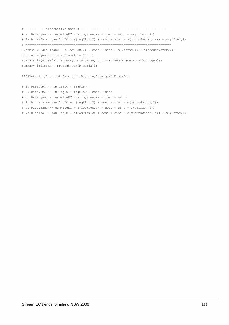
Stream EC trends for inland NSW 2006 233
# ========== Alternative models =================================================
# 7. Data.gam3 <- gam(logEC ~ s(logFlow,2) + cost + sint + s(yrfrac, 4))
# 7a D.gam3a <- gam(logEC ~ s(logFlow,2) + cost + sint + s(groundwater, 4)) + s(yrfrac,2)
# ===============================================================================
D.gam3a <- gam(logEC ~ s(logFlow,2) + cost + sint + s(yrfrac,4) + s(groundwater,2),
control = gam.control(bf.maxit = 100) )
summary.lm(D.gam3a); summary.lm(D.gam3a, corr=F); anova (Data.gam3, D.gam3a)
summary(lm(logEC ~ predict.gam(D.gam3a)))
AIC(Data.lm1,Data.lm2,Data.gam1,D.gam1a,Data.gam3,D.gam3a)
# 1. Data.lm1 <- lm(logEC ~ logFlow )
# 2. Data.lm2 <- lm(logEC ~ logFlow + cost + sint)
# 3. Data.gam1 <- gam(logEC ~ s(logFlow,2) + cost + sint)
# 3a D.gam1a <- gam(logEC ~ s(logFlow,2) + cost + sint + s(groundwater,2))
# 7. Data.gam3 <- gam(logEC ~ s(logFlow,2) + cost + sint + s(yrfrac, 4))
# 7a D.gam3a <- gam(logEC ~ s(logFlow,2) + cost + sint + s(groundwater, 4)) + s(yrfrac,2)

234 Stream EC trends for inland NSW 2006
Appendix 7 – S-PLUS Script Output File
The GREEN numbers in Section 11 (# 11=11=) indicate values which may be useful additions to a summary table for these analyses.
# BLUE text is comment #
# RED text is program code #
# BLACK text is output #
> # ######################################################################################
# These are the models being fitted in this program
#
# 1. Data.lm1 <- lm(logEC ~ logFlow )
# 2. Data.lm2 <- lm(logEC ~ logFlow + cost + sint)
# 3. Data.gam1 <- gam(logEC ~ s(logFlow,2) + cost + sint)
# 3a D.gam1a <- gam(logEC ~ s(logFlow,2) + cost + sint + s(groundwater,2))
# 4. Data.lm3 <- lm(AdjEC ~ yrfrac)
# 5. Data.gam2 <- gam(AdjEC ~ s(yrfrac, 4))
# 6. Data.lm4 <- lm(logEC ~ logFlow + cost + sint + yrfrac)
# 7. Data.gam3 <- gam(logEC ~ s(logFlow,2) + cost + sint + s(yrfrac, 4))
# 7a D.gam3a <- gam(logEC ~ s(logFlow,2) + cost + sint + s(groundwater, 4)) + s(yrfrac,2)
# ######################################################################################
# =1=1=1=1=1=1=1=1=1=1=1=1=1=1=1=1=1=1=1=1=1=1=1=1=1=1=1=1=1=1=1=1=1=1=1=1=1=1=1=1
# ============== Create a "Data" data frame to save having to rename everything ==
# ================================================================================
> Data <- wallallgw # use a common data frame name of Data
> attach(Data) # attach desired data frame
> dim(Data)
[1] 138 7
> Data[1:3, ]
dtime jday instFlow AccVol TumutEC EC76 groundwater
1 02/15/1979 10:00:00.000 28901.42 18.0 1995757 2350 2350 164.819
2 04/12/1979 10:00:00.000 28957.42 30.3 1997038 1700 1700 165.704
3 06/22/1979 11:00:00.000 29028.46 34.6 1999603 1250 1250 165.752
> mon <- months(Data$dtime) # generate vector of months
> yday <- yeardays(Data$dtime) # generate vector of days from start of year
> cost <- cos(((2 * pi * yday)/365)) # dummy variables for season
> sint <- sin(((2 * pi * yday)/365))
> yrfrac <- as.numeric(as.character(years(Data$dtime))) + yday/365
> Data$yrfrac <- yrfrac
> # =2=2=2=2=2=2=2=2=2=2=2=2=2=2=2=2=2=2=2=2=2=2=2=2=2=2=2=2=2=2=2=2=2=2=2=2=
# ============== How regular are the sampling intervals?===================
# =========================================================================

Stream EC trends for inland NSW 2006 235
> mon
[1] Feb Apr Jun Aug Oct Dec Feb Apr Jun Aug Oct Dec Feb Apr Jun Oct Jan Mar
[19] May Jul Oct Jan Mar May Jul Oct Dec Mar Apr Jul Nov Feb Jul Oct Dec Feb
[37] Apr Jun Jul Sep Nov Jan Mar May Jul Sep Nov Jan Mar May Jul Sep Nov Jan
[55] Feb May Jul Sep Nov Jan Apr Jun Aug Oct Mar May Jul Sep Nov Jan Aug Oct
[73] Nov Dec Jan Mar Aug Sep Oct Nov Dec Jan Feb Mar Apr May Jun Jun Oct Nov
[91] Dec Feb Feb Mar Apr May Jun Jul Aug Sep Oct Nov Dec Jan Feb Mar Apr May
[109] Jun Sep Oct Nov Dec Jan Feb Mar Apr May Jun Jul Aug Sep Oct Nov Dec Jan
[127] Feb Mar Apr May Jun Jul Aug Sep Oct Dec Jan Mar
Jan < Feb < Mar < Apr < May < Jun < Jul < Aug < Sep < Oct < Nov < Dec
> diff(yrfrac) * 365 # number of days lapsed between observations
[1] 56 71 55 56 57 69 63 64 56 56 63 54 70 57
[15] 140 76 68 58 63 99 69 61 65 77 91 42 84 60
[29] 65 138 87 166 71 55 64 63 55 49 55 64 57 61
[43] 49 63 63 63 64 70 56 65 56 54 62 43 69 76
[57] 49 85 55 77 77 63 63 126 63 64 70 56 69 1295
[71] 83 27 21 35 57 139 28 36 34 21 34 28 28 35
[85] 28 28 28 119 28 34 36 21 35 28 28 35 28 28
[99] 28 35 21 28 28 28 35 28 21 399 112 35 28 21
[113] 27 28 28 28 35 35 21 35 28 35 35 21 35 28
[127] 28 35 28 29 27 35 36 21 62 35 56
> table(years(dtime), mon) # number of observations per month & year
integer matrix: 23 rows, 12 columns.
Jan Feb Mar Apr May Jun Jul Aug Sep Oct Nov Dec
1979 0 1 0 1 0 1 0 1 0 1 0 1
1980 0 1 0 1 0 1 0 1 0 1 0 1
1981 0 1 0 1 0 1 0 0 0 1 0 0
1982 1 0 1 0 1 0 1 0 0 1 0 0
1983 1 0 1 0 1 0 1 0 0 1 0 1
1984 0 0 1 1 0 0 1 0 0 0 1 0
1985 0 1 0 0 0 0 1 0 0 1 0 1
1986 0 1 0 1 0 1 1 0 1 0 1 0
1987 1 0 1 0 1 0 1 0 1 0 1 0
1988 1 0 1 0 1 0 1 0 1 0 1 0
1989 1 1 0 0 1 0 1 0 1 0 1 0
1990 1 0 0 1 0 1 0 1 0 1 0 0
1991 0 0 1 0 1 0 1 0 1 0 1 0
1992 1 0 0 0 0 0 0 0 0 0 0 0
1995 0 0 0 0 0 0 0 1 0 1 1 1
1996 1 0 1 0 0 0 0 1 1 1 1 1
1997 1 1 1 1 1 2 0 0 0 1 1 1
1998 0 2 1 1 1 1 1 1 1 1 1 1
1999 1 1 1 1 1 0 0 0 0 0 0 0
2000 0 0 0 0 0 1 0 0 1 1 1 1
2001 1 1 1 1 1 1 1 1 1 1 1 1
2002 1 1 1 1 1 1 1 1 1 1 0 1
2003 1 0 1 0 0 0 0 0 0 0 0 0
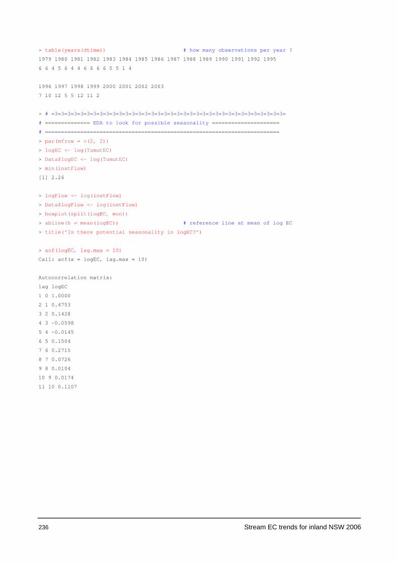
236 Stream EC trends for inland NSW 2006
> table(years(dtime)) # how many observations per year ?
1979 1980 1981 1982 1983 1984 1985 1986 1987 1988 1989 1990 1991 1992 1995
6 6 4 5 6 4 4 6 6 6 6 5 5 1 4
1996 1997 1998 1999 2000 2001 2002 2003
7 10 12 5 5 12 11 2
> # =3=3=3=3=3=3=3=3=3=3=3=3=3=3=3=3=3=3=3=3=3=3=3=3=3=3=3=3=3=3=3=3=3=3=3=3=
# ============== EDA to look for possible seasonality =====================
# =========================================================================
> par(mfrow = c(2, 2))
> logEC <- log(TumutEC)
> Data$logEC <- log(TumutEC)
> min(instFlow)
[1] 2.26
> logFlow <- log(instFlow)
> Data$logFlow <- log(instFlow)
> boxplot(split(logEC, mon))
> abline(h = mean(logEC)) # reference line at mean of log EC
> title("Is there potential seasonality in logEC?")
> acf(logEC, lag.max = 10)
Call: acf(x = logEC, lag.max = 10)
Autocorrelation matrix:
lag logEC
1 0 1.0000
2 1 0.4753
3 2 0.1428
4 3 -0.0598
5 4 -0.0145
6 5 0.1504
7 6 0.2715
8 7 0.0726
9 8 0.0104
10 9 0.0174
11 10 0.1107
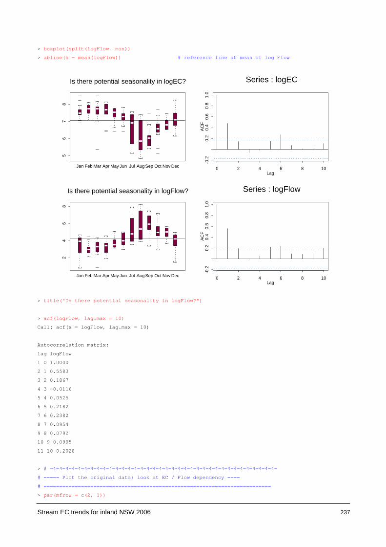
Stream EC trends for inland NSW 2006 237
> boxplot(split(logFlow, mon))
> abline(h = mean(logFlow)) # reference line at mean of log Flow
> title("Is there potential seasonality in logFlow?")
> acf(logFlow, lag.max = 10)
Call: acf(x = logFlow, lag.max = 10)
Autocorrelation matrix:
lag logFlow
1 0 1.0000
2 1 0.5583
3 2 0.1867
4 3 -0.0116
5 4 0.0525
6 5 0.2182
7 6 0.2382
8 7 0.0954
9 8 0.0792
10 9 0.0995
11 10 0.2028
> # =4=4=4=4=4=4=4=4=4=4=4=4=4=4=4=4=4=4=4=4=4=4=4=4=4=4=4=4=4=4=4=4=4=4=4=4=
# ===== Plot the original data; look at EC / Flow dependency ====
# =========================================================================
> par(mfrow = c(2, 1))
56
78
Jan Feb Mar Apr May Jun Jul Aug Sep Oct Nov Dec
Is there potential seasonality in logEC?
Lag
AC
F
0 2 4 6 8 10
-0.2
0.2
0.4
0.6
0.8
1.0
Series : logEC
24
68
Jan Feb Mar Apr May Jun Jul Aug Sep Oct Nov Dec
Is there potential seasonality in logFlow?
Lag
AC
F
0 2 4 6 8 10
-0.2
0.2
0.4
0.6
0.8
1.0
Series : logFlow

238 Stream EC trends for inland NSW 2006
> plot(yrfrac, logEC, type = "b", ylim = c(min(min(logFlow), min(logEC)), max( max(logEC),
max(logFlow))))
> title("log(EC) open circles; log(Flow) solid green circles") # plot original EC data open circles
> abline(h = mean(logEC)) # reference line at mean of log EC
> points(yrfrac, logFlow, col = 4, pch = 10, type = "b") # overlay the log Flow solid green
> abline(h = mean(logFlow))
> plot(logFlow, logEC, pch = 15) # look at log(Flow)/log(EC)
relationship
> title("must correct log(EC) to a constant log(Flow)")
> # =5=5=5=5=5=5=5=5=5=5=5=5=5=5=5=5=5=5=5=5=5=5=5=5=5=5=5=5=5=5=5=5=5=5=5=5=
# ===== Start with a linear model on log scale =================
# ===== ... then add sin & cos terms =================
# ===== ... then try adding spline(instFlow) =================
# ========================================================================
> Data.lm1 <- lm(logEC ~ logFlow)
> Data.lm2 <- lm(logEC ~ logFlow + cost + sint)
> Data.gam1 <- gam(logEC ~ s(logFlow, 2) + cost + sint)
> Data.lm2a <- lm(logEC ~ cost + sint)
> Data$season <- predict(Data.lm2a)
> summary(Data.lm1, corr = F); anova(Data.lm1) # original linear model
Call: lm(formula = logEC ~ logFlow)
Residuals:
Min 1Q Median 3Q Max
-1.828 -0.1164 0.04352 0.1972 0.6607
yrfrac
logE
C
1980 1985 1990 1995 2000
24
68
log(EC) open circles; log(Flow) solid green circles
logFlow
logE
C
2 4 6 8
56
78
must correct log(EC) to a constant log(Flow)

Stream EC trends for inland NSW 2006 239
Coefficients:
Value Std. Error t value Pr(>|t|)
(Intercept) 9.2488 0.0842 109.8285 0.0000
logFlow -0.5171 0.0189 -27.4275 0.0000
Residual standard error: 0.3132 on 136 degrees of freedom
0Multiple R-Squared: 0.8469
F-statistic: 752.3 on 1 and 136 degrees of freedom, the p-value is 0
Analysis of Variance Table
Response: logEC
Terms added sequentially (first to last)
Df Sum of Sq Mean Sq F Value Pr(F)
logFlow 1 73.77783 73.77783 752.2702 0
Residuals 136 13.33801 0.09807
> summary(Data.lm2, corr = F); anova(Data.lm1, Data.lm2) # adding staggered
Call: lm(formula = logEC ~ logFlow + cost + sint)
Residuals:
Min 1Q Median 3Q Max
-1.877 -0.1055 0.03911 0.1861 0.622
Coefficients:
Value Std. Error t value Pr(>|t|)
(Intercept) 9.1660 0.1125 81.4738 0.0000
logFlow -0.4982 0.0254 -19.5840 0.0000
cost 0.0274 0.0400 0.6847 0.4947
sint 0.0507 0.0497 1.0213 0.3090
Residual standard error: 0.314 on 134 degrees of freedom
Multiple R-Squared: 0.8483
F-statistic: 249.8 on 3 and 134 degrees of freedom, the p-value is 0
Analysis of Variance Table
Response: logEC
Terms Resid. Df RSS Test Df Sum of Sq F Value Pr(F)
1 logFlow 136 13.33801
2 logFlow + cost + sint 134 13.21405 +cost+sint 2 0.1239577 0.6285104 0.5349506
> summary(Data.gam1, corr = F); anova(Data.lm2, Data.gam1) # adding spline for inst Flow
Call: gam(formula = logEC ~ s(logFlow, 2) + cost + sint)
Deviance Residuals:
Min 1Q Median 3Q Max
-1.899777 -0.08394454 0.04062478 0.1687246 0.6001848
(Dispersion Parameter for Gaussian family taken to be 0.0964553 )

240 Stream EC trends for inland NSW 2006
Null Deviance: 87.11584 on 137 degrees of freedom
Residual Deviance: 12.82857 on 133.0002 degrees of freedom
Number of Local Scoring Iterations: 1
DF for Terms and Chi-squares for Nonparametric Effects
Df Npar Df Npar Chisq P(Chi)
(Intercept) 1
s(logFlow, 2) 1 1 3.996404 0.04558675
cost 1
sint 1
Analysis of Variance Table
Response: logEC
Terms Resid. Df RSS Test Df Sum of Sq F Value Pr(F)
1 logFlow + cost + sint 134.0000 13.21405
2 s(logFlow, 2) + cost + sint 133.0002 12.82857 1 vs. 2 0.9998424 0.3854744 3.997034 0.04762443
> summary.lm(Data.gam1)
Call: gam(formula = logEC ~ s(logFlow, 2) + cost + sint)
Residuals:
Min 1Q Median 3Q Max
-1.9 -0.08394 0.04062 0.1687 0.6002
Coefficients:
Value Std. Error t value Pr(>|t|)
(Intercept) 9.1691 0.1113 82.4082 0.0000
s(logFlow, 2) -0.4989 0.0252 -19.8319 0.0000
cost 0.0288 0.0396 0.7272 0.4684
sint 0.0477 0.0491 0.9711 0.3333
Residual standard error: 0.3106 on 133.000157644148 degrees of freedom
Multiple R-Squared: 0.8501
F-statistic: 256.3 on 3 and 133.000157644148 degrees of freedom, the p-value is 0
Correlation of Coefficients:
(Intercept) s(logFlow, 2) cost
s(logFlow, 2) -0.9711
cost -0.3413 0.3287
sint -0.6291 0.6427 0.2295
> summary(lm(logEC ~ predict.gam(Data.gam1)))
Call: lm(formula = logEC ~ predict.gam(Data.gam1))
Residuals:
Min 1Q Median 3Q Max

Stream EC trends for inland NSW 2006 241
-1.9 -0.08393 0.04004 0.1688 0.6005
Coefficients:
Value Std. Error t value Pr(>|t|)
(Intercept) -0.0110 0.2532 -0.0433 0.9655
predict.gam(Data.gam1) 1.0016 0.0357 28.0634 0.0000
Residual standard error: 0.3071 on 136 degrees of freedom
Multiple R-Squared: 0.8527
F-statistic: 787.6 on 1 and 136 degrees of freedom, the p-value is 0
Correlation of Coefficients:
(Intercept)
predict.gam(Data.gam1) -0.9947
> # =6=6=6=6=6=6=6=6=6=6=6=6=6=6=6=6=6=6=6=6=6=6=6=6=6=6=6=6=6=6=6=6=6=6=6=6=
# ======= Which model seems more appropriate with smallest AIC ============
# =========================================================================
> AIC(Data.lm1, Data.lm2, Data.lm2a, Data.gam1)
df AIC
Data.lm1 3 75.17125
Data.lm2 5 77.88274
Data.lm2a 4 262.35254
Data.gam1 5 73.79718
> par(mfrow = c(1, 1))
> acf(Data.gam1$residuals, lag.max = 10)
Call: acf(x = Data.gam1$residuals, lag.max = 10)
Autocorrelation matrix:
lag Data.gam1
1 0 1.0000
2 1 0.1693
3 2 0.0481
4 3 0.0600
5 4 0.0184
6 5 -0.0094
7 6 0.0515
8 7 0.1056
9 8 0.0466
10 9 0.0303
11 10 0.0355

242 Stream EC trends for inland NSW 2006
Lag
ACF
0 2 4 6 8 10
-0.2
0.0
0.2
0.4
0.6
0.8
1.0
Series : Data.gam1$residuals

Stream EC trends for inland NSW 2006 243
> # =7=7=7=7=7=7=7=7=7=7=7=7=7=7=7=7=7=7=7=7=7=7=7=7=7=7=7=7=7=7=7=7=7=7=7=7=
# ======= Create a plot of these models ===================================
# =========================================================================
> plot(logFlow, logEC) # plot the original data
> title("Black=linear; Red=F+s+c; Orange=s(Flow,2)+s+c")
> abline(Data.lm2, col = 3, lwd = 4) # red line is Flow + sin + cos
# create data frame for prediction
> dummy <- data.frame(cost = rep(mean(cost), length(cost)))
> dummy$sint <- rep(mean(sint), length(sint))
> dummy$logFlow <- logFlow
> dummy$gam1 <- predict.gam(Data.gam1, dummy, type = "response")
> points(logFlow, dummy$gam1, col = 5, lwd = 4) # orange points are smoothed Flow
logFlow
logE
C
2 4 6 8
56
78
Black=linear; Red=F+s+c; Orange=s(Flow,2)+s+c

244 Stream EC trends for inland NSW 2006
> # =8=8=8=8=8=8=8=8=8=8=8=8=8=8=8=8=8=8=8=8=8=8=8=8=8=8=8=8=8=8=8=8=8=8=8=8=
# ===== Look at adjusted EC versus time, adjusted for Flow & Seasonality ===
# ========================================================================
> par(mfrow = c(2, 1))
> AdjEC <- mean(logEC) + Data.gam1$residuals
> Data$AdjEC = AdjEC
> # plot(yrfrac,logEC)
> plot(yrfrac, AdjEC, pch = 16) # now plot EC adjusted for Flow &
Seasonality
> abline(h = mean(logEC)) # add reference line at mean of log EC
> lines(lowess(yrfrac, AdjEC), col = 3, lwd = 4) # show a lowess smoother over time
> title("EC adjusted for Flow & Seasonality; lowess smoother over time")
> plot(groundwater, AdjEC, pch = 16) # now plot EC adjusted for Flow &
Groundwater
> abline(h = mean(logEC)) # add reference line at mean of log EC
> lines(lowess(groundwater, AdjEC), col = 3, lwd = 4) # show a lowess smoother over time
> title("EC adjusted for Flow & Seasonality; lowess smoother over groundwater")
yrfrac
Adj
EC
1980 1985 1990 1995 2000
5.5
6.0
6.5
7.0
7.5
EC adjusted for Flow & Seasonality; lowess smoother over time
groundwater
Adj
EC
166 168 170
5.5
6.0
6.5
7.0
7.5
EC adjusted for Flow & Seasonality; lowess smoother over groundwater

Stream EC trends for inland NSW 2006 245
> # =9=9=9=9=9=9=9=9=9=9=9=9=9=9=9=9=9=9=9=9=9=9=9=9=9=9=9=9=9=9=9=9=9=9=9=9=
# ===== Fit Generalized Additive Model to adjusted EC data over time ======
# ===== and plot the linear and {linear + smooth} spline components =======
# =========================================================================
> Data.lm3 <- lm(AdjEC ~ yrfrac)
> Data.gam2 <- gam(AdjEC ~ s(yrfrac, 4))
# Following line added by FJH
> Data$Data.gam2 <- predict.gam(Data.gam2) # addition FJH 4th June
> summary(Data.lm3)
Call: lm(formula = AdjEC ~ yrfrac)
Residuals:
Min 1Q Median 3Q Max
-1.888 -0.1162 0.04685 0.1882 0.7018
Coefficients:
Value Std. Error t value Pr(>|t|)
(Intercept) -11.8912 6.6213 -1.7959 0.0747
yrfrac 0.0095 0.0033 2.8619 0.0049
Residual standard error: 0.2983 on 136 degrees of freedom
Multiple R-Squared: 0.0568
F-statistic: 8.19 on 1 and 136 degrees of freedom, the p-value is 0.004878
Correlation of Coefficients:
(Intercept)
yrfrac -1
> summary(Data.gam2)
Call: gam(formula = AdjEC ~ s(yrfrac, 4))
Deviance Residuals:
Min 1Q Median 3Q Max
-1.940155 -0.115644 0.05524887 0.1766916 0.727667
(Dispersion Parameter for Gaussian family taken to be 0.0888215 )
Null Deviance: 12.82857 on 137 degrees of freedom
Residual Deviance: 11.81326 on 133.0001 degrees of freedom
Number of Local Scoring Iterations: 1
DF for Terms and F-values for Nonparametric Effects
Df Npar Df Npar F Pr(F)
(Intercept) 1
s(yrfrac, 4) 1 3 1.075704 0.3617306
> summary.lm(Data.gam2)

246 Stream EC trends for inland NSW 2006
Call: gam(formula = AdjEC ~ s(yrfrac, 4))
Residuals:
Min 1Q Median 3Q Max
-1.94 -0.1156 0.05525 0.1767 0.7277
Coefficients:
Value Std. Error t value Pr(>|t|)
(Intercept) -11.8912 6.6158 -1.7974 0.0745
s(yrfrac, 4) 0.0095 0.0033 2.8643 0.0049
Residual standard error: 0.298 on 133.000097500532 degrees of freedom
Multiple R-Squared: 0.07181
F-statistic: 10.9 on 1 and 133.000097500532 degrees of freedom, the p-value is 0.001234
Correlation of Coefficients:
(Intercept)
s(yrfrac, 4) -1
> #plot(Data.gam2, se=T)
> #abline(h=0) # add reference line at zero
> #title("aberall -Zero is the mean (Flow adjusted EC)")
> plot(yrfrac, AdjEC) # Plot EC adjusted for Flow &
Seasonality
> abline(h = mean(logEC)) # add reference line at mean of log EC
> lines(yrfrac, predict(Data.lm3), col = 4, lwd = 4) # show the linear part in green
> lines(yrfrac, predict.gam(Data.gam2), col = 5, lwd = 4) # add the GAM fitted model in orange
> title("Adjusted EC data: Green is linear fit; Orange is spline")
> #acf(Data.gam2$residuals,lag.max=10) # check for autocorrelation in residuals
> D.lm3a <- lm(AdjEC ~ groundwater)
> D.gam2a <- gam(AdjEC ~ s(groundwater, 2))
> summary(D.lm3a)
Call: lm(formula = AdjEC ~ groundwater)
Residuals:
Min 1Q Median 3Q Max
-1.932 -0.1294 0.05291 0.1798 0.6843
Coefficients:
Value Std. Error t value Pr(>|t|)
(Intercept) 0.4098 1.9852 0.2064 0.8368
groundwater 0.0393 0.0117 3.3492 0.0010
Residual standard error: 0.2952 on 136 degrees of freedom
Multiple R-Squared: 0.07619
F-statistic: 11.22 on 1 and 136 degrees of freedom, the p-value is 0.001049
Correlation of Coefficients:
(Intercept)
groundwater -0.9999
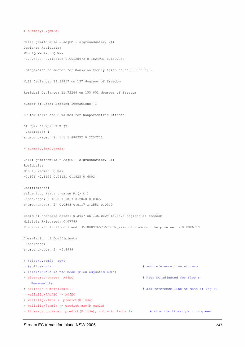
Stream EC trends for inland NSW 2006 247
> summary(D.gam2a)
Call: gam(formula = AdjEC ~ s(groundwater, 2))
Deviance Residuals:
Min 1Q Median 3Q Max
-1.925528 -0.1125483 0.06120973 0.1824931 0.6802358
(Dispersion Parameter for Gaussian family taken to be 0.0868339 )
Null Deviance: 12.82857 on 137 degrees of freedom
Residual Deviance: 11.72266 on 135.001 degrees of freedom
Number of Local Scoring Iterations: 1
DF for Terms and F-values for Nonparametric Effects
Df Npar Df Npar F Pr(F)
(Intercept) 1
s(groundwater, 2) 1 1 1.480972 0.2257211
> summary.lm(D.gam2a)
Call: gam(formula = AdjEC ~ s(groundwater, 2))
Residuals:
Min 1Q Median 3Q Max
-1.926 -0.1125 0.06121 0.1825 0.6802
Coefficients:
Value Std. Error t value Pr(>|t|)
(Intercept) 0.4098 1.9817 0.2068 0.8365
s(groundwater, 2) 0.0393 0.0117 3.3551 0.0010
Residual standard error: 0.2947 on 135.000976573578 degrees of freedom
Multiple R-Squared: 0.07789
F-statistic: 12.12 on 1 and 135.000976573578 degrees of freedom, the p-value is 0.0006719
Correlation of Coefficients:
(Intercept)
s(groundwater, 2) -0.9999
> #plot(D.gam2a, se=T)
> #abline(h=0) # add reference line at zero
> #title("Zero is the mean (Flow adjusted EC)")
> plot(groundwater, AdjEC) # Plot EC adjusted for Flow &
Seasonality
> abline(h = mean(logEC)) # add reference line at mean of log EC
> wallallgw$AdjEC <- AdjEC
> wallallgw$lm3a <- predict(D.lm3a)
> wallallgw$gam2a <- predict.gam(D.gam2a)
> lines(groundwater, predict(D.lm3a), col = 4, lwd = 4) # show the linear part in green
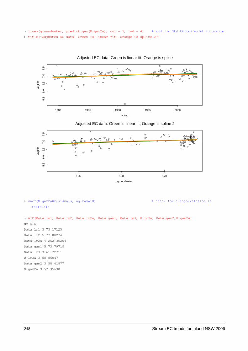
248 Stream EC trends for inland NSW 2006
> lines(groundwater, predict.gam(D.gam2a), col = 5, lwd = 4) # add the GAM fitted model in orange
> title("Adjusted EC data: Green is linear fit; Orange is spline 2")
> #acf(D.gam2a$residuals,lag.max=10) # check for autocorrelation in
residuals
> AIC(Data.lm1, Data.lm2, Data.lm2a, Data.gam1, Data.lm3, D.lm3a, Data.gam2,D.gam2a)
df AIC
Data.lm1 3 75.17125
Data.lm2 5 77.88274
Data.lm2a 4 262.35254
Data.gam1 5 73.79718
Data.lm3 3 61.72711
D.lm3a 3 58.86047
Data.gam2 3 58.41877
D.gam2a 3 57.35630
yrfrac
Adj
EC
1980 1985 1990 1995 2000
5.5
6.0
6.5
7.0
7.5
Adjusted EC data: Green is linear fit; Orange is spline
groundwater
Adj
EC
166 168 170
5.5
6.0
6.5
7.0
7.5
Adjusted EC data: Green is linear fit; Orange is spline 2
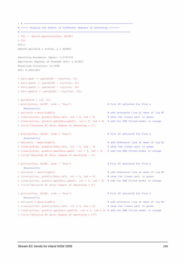
Stream EC trends for inland NSW 2006 249
> # =========================================================================
# ===== display the effect of different degrees of smoothing =======
# =========================================================================
> fit <- smooth.spline(yrfrac, AdjEC)
> fit
Call:
smooth.spline(x = yrfrac, y = AdjEC)
Smoothing Parameter (Spar): 0.5722725
Equivalent Degrees of Freedom (Df): 2.413857
Penalized Criterion: 12.0448
GCV: 0.09012851
> Data.gam2 <- gam(AdjEC ~ s(yrfrac, 4))
> Data.gam22 <- gam(AdjEC ~ s(yrfrac, 2))
> Data.gam26 <- gam(AdjEC ~ s(yrfrac, 6))
> Data.gam210 <- gam(AdjEC ~ s(yrfrac, 10))
> par(mfrow = c(2, 2))
> plot(yrfrac, AdjEC, xlab = "Year") # Plot EC adjusted for Flow &
Seasonality
> abline(h = mean(logEC)) # add reference line at mean of log EC
> lines(yrfrac, predict(Data.lm3), col = 4, lwd = 4) # show the linear part in green
> lines(yrfrac, predict.gam(Data.gam22), col = 5, lwd = 4) # add the GAM fitted model in orange
> title("Adjusted EC data: Degree of smoothing = 2")
> plot(yrfrac, AdjEC, xlab = "Year") # Plot EC adjusted for Flow &
Seasonality
> abline(h = mean(logEC)) # add reference line at mean of log EC
> lines(yrfrac, predict(Data.lm3), col = 4, lwd = 4) # show the linear part in green
> lines(yrfrac, predict.gam(Data.gam2), col = 5, lwd = 4) # add the GAM fitted model in orange
> title("Adjusted EC data: Degree of smoothing = 4")
> plot(yrfrac, AdjEC, xlab = "Year") # Plot EC adjusted for Flow &
Seasonality
> abline(h = mean(logEC)) # add reference line at mean of log EC
> lines(yrfrac, predict(Data.lm3), col = 4, lwd = 4) # show the linear part in green
> lines(yrfrac, predict.gam(Data.gam26), col = 5, lwd = 4) # add the GAM fitted model in orange
> title("Adjusted EC data: Degree of smoothing = 6")
> plot(yrfrac, AdjEC, xlab = "Year") # Plot EC adjusted for Flow &
Seasonality
> abline(h = mean(logEC)) # add reference line at mean of log EC
> lines(yrfrac, predict(Data.lm3), col = 4, lwd = 4) # show the linear part in green
> lines(yrfrac, predict.gam(Data.gam210), col = 5, lwd = 4) # add the GAM fitted model in orange
> title("Adjusted EC data: Degree of smoothing = 10")
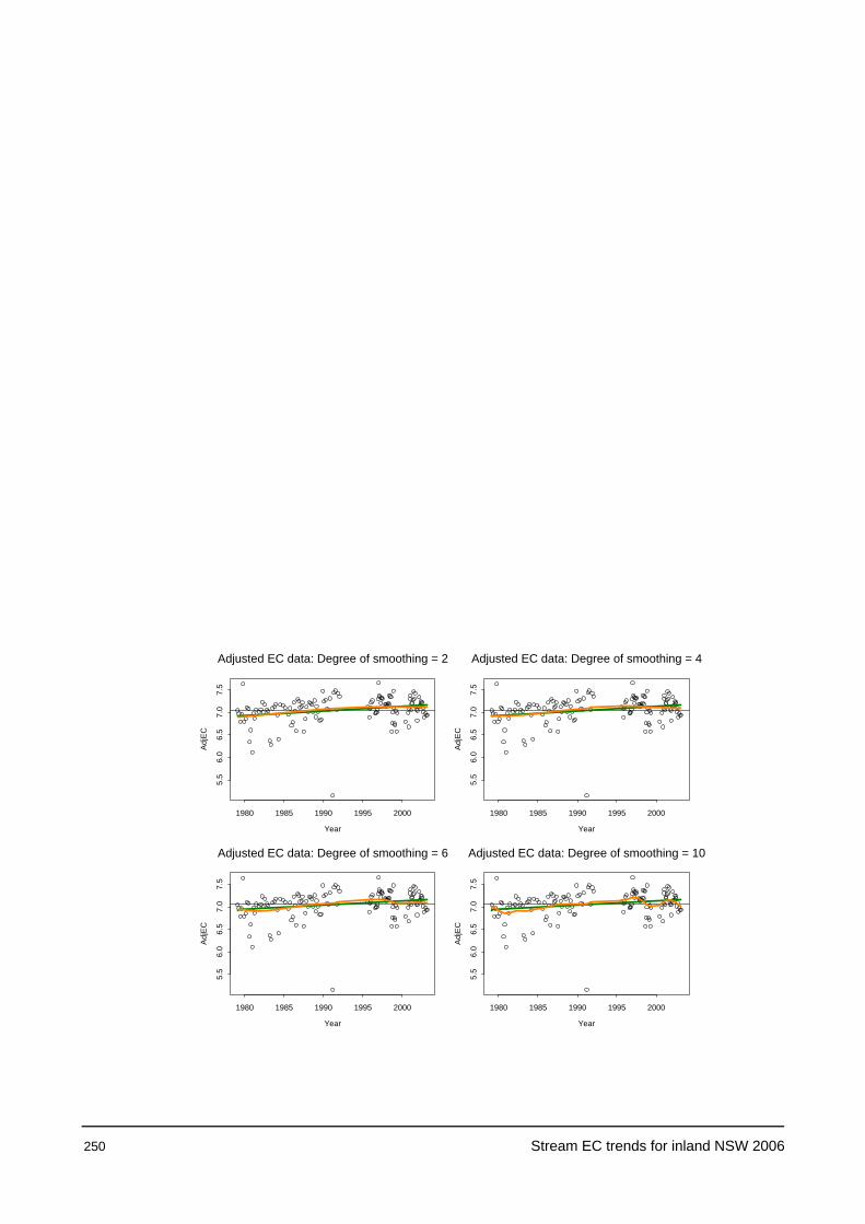
250 Stream EC trends for inland NSW 2006
Year
Adj
EC
1980 1985 1990 1995 2000
5.5
6.0
6.5
7.0
7.5
Adjusted EC data: Degree of smoothing = 2
Year
Adj
EC
1980 1985 1990 1995 2000
5.5
6.0
6.5
7.0
7.5
Adjusted EC data: Degree of smoothing = 4
Year
Adj
EC
1980 1985 1990 1995 2000
5.5
6.0
6.5
7.0
7.5
Adjusted EC data: Degree of smoothing = 6
Year
Adj
EC
1980 1985 1990 1995 2000
5.5
6.0
6.5
7.0
7.5
Adjusted EC data: Degree of smoothing = 10
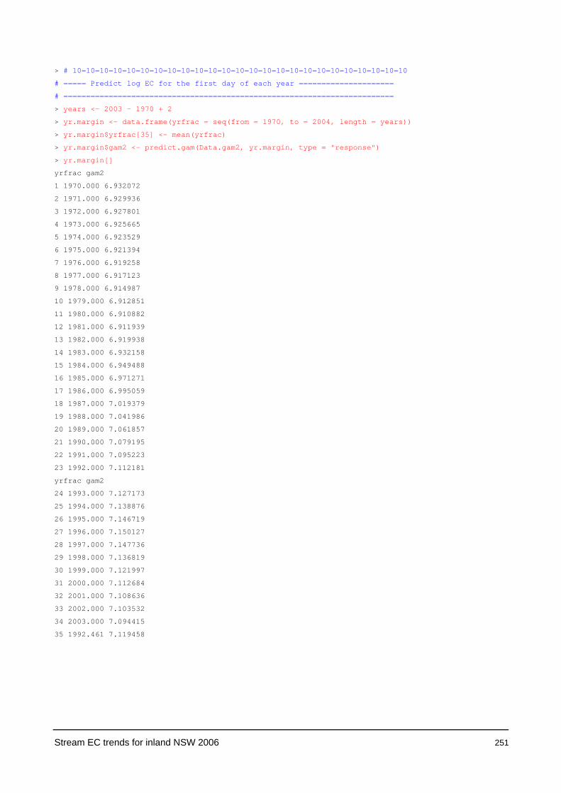
Stream EC trends for inland NSW 2006 251
> # 10=10=10=10=10=10=10=10=10=10=10=10=10=10=10=10=10=10=10=10=10=10=10=10=10
# ===== Predict log EC for the first day of each year =====================
# =========================================================================
> years <- 2003 - 1970 + 2
> yr.margin <- data.frame(yrfrac = seq(from = 1970, to = 2004, length = years))
> yr.margin$yrfrac[35] <- mean(yrfrac)
> yr.margin$gam2 <- predict.gam(Data.gam2, yr.margin, type = "response")
> yr.margin[]
yrfrac gam2
1 1970.000 6.932072
2 1971.000 6.929936
3 1972.000 6.927801
4 1973.000 6.925665
5 1974.000 6.923529
6 1975.000 6.921394
7 1976.000 6.919258
8 1977.000 6.917123
9 1978.000 6.914987
10 1979.000 6.912851
11 1980.000 6.910882
12 1981.000 6.911939
13 1982.000 6.919938
14 1983.000 6.932158
15 1984.000 6.949488
16 1985.000 6.971271
17 1986.000 6.995059
18 1987.000 7.019379
19 1988.000 7.041986
20 1989.000 7.061857
21 1990.000 7.079195
22 1991.000 7.095223
23 1992.000 7.112181
yrfrac gam2
24 1993.000 7.127173
25 1994.000 7.138876
26 1995.000 7.146719
27 1996.000 7.150127
28 1997.000 7.147736
29 1998.000 7.136819
30 1999.000 7.121997
31 2000.000 7.112684
32 2001.000 7.108636
33 2002.000 7.103532
34 2003.000 7.094415
35 1992.461 7.119458
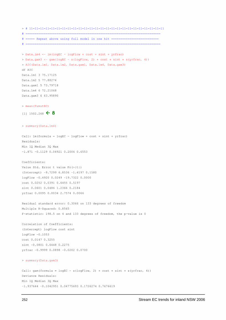
252 Stream EC trends for inland NSW 2006
> # 11=11=11=11=11=11=11=11=11=11=11=11=11=11=11=11=11=11=11=11=11=11=11=11=11
# ==========================================================================
# ===== Repeat above using full model in one hit ==========================
# ==========================================================================
> Data.lm4 <- lm(logEC ~ logFlow + cost + sint + yrfrac)
> Data.gam3 <- gam(logEC ~ s(logFlow, 2) + cost + sint + s(yrfrac, 4))
> AIC(Data.lm1, Data.lm2, Data.gam1, Data.lm4, Data.gam3)
df AIC
Data.lm1 3 75.17125
Data.lm2 5 77.88274
Data.gam1 5 73.79718
Data.lm4 6 72.21068
Data.gam3 6 63.95890
> mean(TumutEC)
[1] 1502.268 8
> summary(Data.lm4)
Call: lm(formula = logEC ~ logFlow + cost + sint + yrfrac)
Residuals:
Min 1Q Median 3Q Max
-1.871 -0.1129 0.04921 0.2006 0.6553
Coefficients:
Value Std. Error t value Pr(>|t|)
(Intercept) -9.7299 6.8536 -1.4197 0.1580
logFlow -0.4920 0.0249 -19.7322 0.0000
cost 0.0252 0.0391 0.6455 0.5197
sint 0.0601 0.0486 1.2366 0.2184
yrfrac 0.0095 0.0034 2.7574 0.0066
Residual standard error: 0.3066 on 133 degrees of freedom
Multiple R-Squared: 0.8565
F-statistic: 198.5 on 4 and 133 degrees of freedom, the p-value is 0
Correlation of Coefficients:
(Intercept) logFlow cost sint
logFlow -0.1053
cost 0.0147 0.3255
sint -0.0801 0.6448 0.2275
yrfrac -0.9999 0.0898 -0.0202 0.0700
> summary(Data.gam3)
Call: gam(formula = logEC ~ s(logFlow, 2) + cost + sint + s(yrfrac, 4))
Deviance Residuals:
Min 1Q Median 3Q Max
-1.937644 -0.1042951 0.04775693 0.1726274 0.7676619

Stream EC trends for inland NSW 2006 253
(Dispersion Parameter for Gaussian family taken to be 0.0912708 )
Null Deviance: 87.11584 on 137 degrees of freedom
Residual Deviance: 11.77396 on 129.0003 degrees of freedom
Number of Local Scoring Iterations: 1
DF for Terms and F-values for Nonparametric Effects
Df Npar Df Npar F Pr(F)
(Intercept) 1
s(logFlow, 2) 1 1 3.916259 0.0499573 6
cost 1
sint 1
s(yrfrac, 4) 1 3 1.185677 0.3178680 5

254 Stream EC trends for inland NSW 2006
> summary.lm(Data.gam3)
Call: gam(formula = logEC ~ s(logFlow, 2) + cost + sint + s(yrfrac, 4))
Residuals:
Min 1Q Median 3Q Max
-1.938 -0.1043 0.04776 0.1726 0.7677
Coefficients:
Value Std. Error t value Pr(>|t|)
(Intercept) -9.3717 6.7540 -1.3876 0.1677
s(logFlow, 2) -0.5164 0.0246 -21.0140 0.0000
cost 0.0129 0.0385 0.3345 0.7386
sint 0.0310 0.0479 0.6480 0.5181
s(yrfrac, 4) 0.0093 0.0034 2.7605 0.0066
--------------1------2------------3-----
Residual standard error: 0.3021 on 129.00025514468 degrees of freedom
Multiple R-Squared: 0.8611
F-statistic: 205.9 on 4 and 129.00025514468 degrees of freedom, the p-value is 0
Correlation of Coefficients:
(Intercept) s(logFlow, 2) cost sint
s(logFlow, 2) -0.1053
cost 0.0147 0.3255
sint -0.0801 0.6448 0.2275
s(yrfrac, 4) -0.9999 0.0898 -0.0202 0.0700
> Data.gam4 <- gam(logEC ~ s(logFlow, 2) + s(yrfrac, 4))
> anova(Data.gam4, Data.gam3) # shows additional reduction in deviance due to Sin &
Cos
Analysis of Deviance Table
Response: logEC
Terms Resid. Df Resid. Dev Test Df Deviance
1 s(logFlow, 2) + s(yrfrac, 4) 131.0003 11.80148
2 s(logFlow, 2) + cost + sint + s(yrfrac, 4) 129.0003 11.77396 +cost+sint 2 0.02751376 7
> summary(lm(logEC ~ predict.gam(Data.gam3)))
Call: lm(formula = logEC ~ predict.gam(Data.gam3))
Residuals:
Min 1Q Median 3Q Max
-1.938 -0.104 0.04588 0.1718 0.7711
Coefficients:
Value Std. Error t value Pr(>|t|)
(Intercept) -0.0154 0.2411 -0.0637 0.9493
predict.gam(Data.gam3) 1.0022 0.0340 29.5008 0.0000

Stream EC trends for inland NSW 2006 255
Residual standard error: 0.2942 on 136 degrees of freedom
Multiple R-Squared: 0.8649
F-statistic: 870.3 on 1 and 136 degrees of freedom, the p-value is 0
Correlation of Coefficients:
(Intercept)
predict.gam(Data.gam3) -0.9946
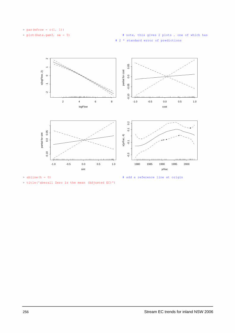
256 Stream EC trends for inland NSW 2006
> par(mfrow = c(1, 1))
> plot(Data.gam3, se = T) # note, this gives 2 plots , one of which has
# 2 * standard error of predictions
> abline(h = 0) # add a reference line at origin
> title("aberall Zero is the mean (Adjusted EC)")
logFlow
s(lo
gFlo
w, 2
)
2 4 6 8
-2-1
01
2
cost
parti
al fo
r cos
t
-1.0 -0.5 0.0 0.5 1.0
-0.1
0-0
.05
0.0
0.05
sint
parti
al fo
r sin
t
-1.0 -0.5 0.0 0.5 1.0
-0.1
00.
00.
05
yrfrac
s(yr
frac,
4)
1980 1985 1990 1995 2000
-0.3
-0.1
0.1
0.2
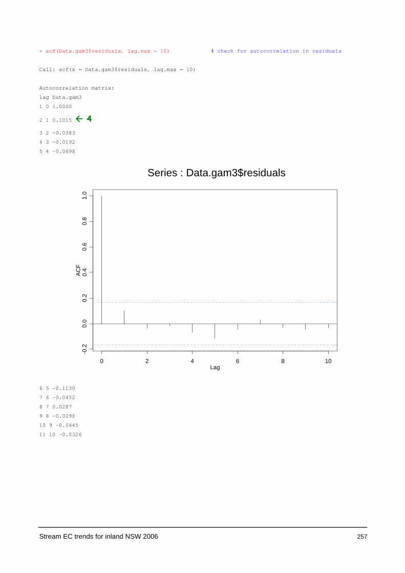
Stream EC trends for inland NSW 2006 257
> acf(Data.gam3$residuals, lag.max = 10) # check for autocorrelation in residuals
Call: acf(x = Data.gam3$residuals, lag.max = 10)
Autocorrelation matrix:
lag Data.gam3
1 0 1.0000
2 1 0.1015 4
3 2 -0.0383
4 3 -0.0192
5 4 -0.0698
6 5 -0.1130
7 6 -0.0452
8 7 0.0287
9 8 -0.0298
10 9 -0.0445
11 10 -0.0326
Lag
ACF
0 2 4 6 8 10
-0.2
0.0
0.2
0.4
0.6
0.8
1.0
Series : Data.gam3$residuals

258 Stream EC trends for inland NSW 2006
> # 12=12=12=12=12=12=12=12=12=12=12=12=12=12=12=12=12=12=12=12=12=12=12=12=12
# == Plot original data, =============================
# == ..... then Data.gam1 <- gam(logEC ~ s(logFlow,2) + cost + sint) ===================
# == ..... then Data.gam3 <- gam(logEC ~ s(logFlow,2) + cost + sint + s(yrfrac, 4)) ====
# == ..... therefore, Data.gam3 - Data.gam1 = {linear + smooth} * yrfrac component
# == ..... but must add on the grand mean, back to proper scale ==============================
#
================================================================================================
===
> smoothEC <- mean(logEC) + predict.gam(Data.gam3) - predict.gam(Data.gam1)
> plot(yrfrac, logEC) # plot original data
> abline(h = mean(logEC)) # add a reference line at mean
> title("original log(EC); Red: gam1; Green: gam3; Orange: smooth yrfrac trend")
> title(sub = "BLUE curve is from fitting AdjEC ~ s(yrfrac,4) in 2-step approach")
> lines(yrfrac, predict.gam(Data.gam1), col = 3) # add RED fitted curve from
spline(Flow,2)+s+c
> lines(yrfrac, predict.gam(Data.gam2), col = 6, lwd = 4) # add BLUE fitted from 2 step approach
> lines(yrfrac, predict.gam(Data.gam3), col = 4) # add GREEN curve: spl(Flow,2)+s+c +
spl(yrfrac,4)
> lines(yrfrac, smoothEC, col = 5, lwd = 4) # show the smoothed part
yrfrac
logE
C
1980 1985 1990 1995 2000
56
78
original log(EC); Red: gam1; Green: gam3; Orange: smooth yrfrac trend
BLUE curve is from fitting AdjEC ~ s(yrfrac,4) in 2-step approach
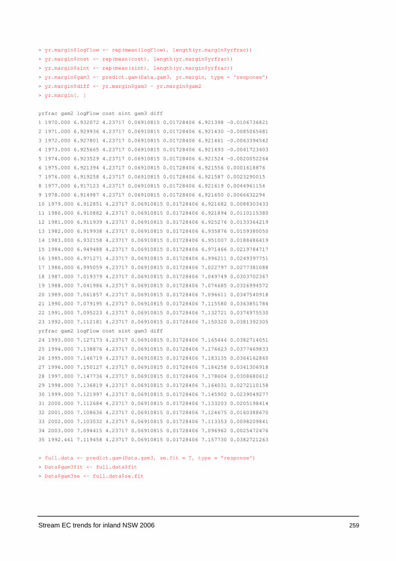
Stream EC trends for inland NSW 2006 259
> yr.margin$logFlow <- rep(mean(logFlow), length(yr.margin$yrfrac))
> yr.margin$cost <- rep(mean(cost), length(yr.margin$yrfrac))
> yr.margin$sint <- rep(mean(sint), length(yr.margin$yrfrac))
> yr.margin$gam3 <- predict.gam(Data.gam3, yr.margin, type = "response")
> yr.margin$diff <- yr.margin$gam3 - yr.margin$gam2
> yr.margin[, ]
yrfrac gam2 logFlow cost sint gam3 diff
1 1970.000 6.932072 4.23717 0.06910815 0.01728406 6.921398 -0.0106736821
2 1971.000 6.929936 4.23717 0.06910815 0.01728406 6.921430 -0.0085065681
3 1972.000 6.927801 4.23717 0.06910815 0.01728406 6.921461 -0.0063394542
4 1973.000 6.925665 4.23717 0.06910815 0.01728406 6.921493 -0.0041723403
5 1974.000 6.923529 4.23717 0.06910815 0.01728406 6.921524 -0.0020052264
6 1975.000 6.921394 4.23717 0.06910815 0.01728406 6.921556 0.0001618876
7 1976.000 6.919258 4.23717 0.06910815 0.01728406 6.921587 0.0023290015
8 1977.000 6.917123 4.23717 0.06910815 0.01728406 6.921619 0.0044961154
9 1978.000 6.914987 4.23717 0.06910815 0.01728406 6.921650 0.0066632294
10 1979.000 6.912851 4.23717 0.06910815 0.01728406 6.921682 0.0088303433
11 1980.000 6.910882 4.23717 0.06910815 0.01728406 6.921894 0.0110115380
12 1981.000 6.911939 4.23717 0.06910815 0.01728406 6.925276 0.0133364219
13 1982.000 6.919938 4.23717 0.06910815 0.01728406 6.935876 0.0159380050
14 1983.000 6.932158 4.23717 0.06910815 0.01728406 6.951007 0.0188486419
15 1984.000 6.949488 4.23717 0.06910815 0.01728406 6.971466 0.0219784717
16 1985.000 6.971271 4.23717 0.06910815 0.01728406 6.996211 0.0249397751
17 1986.000 6.995059 4.23717 0.06910815 0.01728406 7.022797 0.0277381088
18 1987.000 7.019379 4.23717 0.06910815 0.01728406 7.049749 0.0303702367
19 1988.000 7.041986 4.23717 0.06910815 0.01728406 7.074685 0.0326994572
20 1989.000 7.061857 4.23717 0.06910815 0.01728406 7.096611 0.0347540918
21 1990.000 7.079195 4.23717 0.06910815 0.01728406 7.115580 0.0363851784
22 1991.000 7.095223 4.23717 0.06910815 0.01728406 7.132721 0.0374975530
23 1992.000 7.112181 4.23717 0.06910815 0.01728406 7.150320 0.0381392305
yrfrac gam2 logFlow cost sint gam3 diff
24 1993.000 7.127173 4.23717 0.06910815 0.01728406 7.165444 0.0382714051
25 1994.000 7.138876 4.23717 0.06910815 0.01728406 7.176623 0.0377469833
26 1995.000 7.146719 4.23717 0.06910815 0.01728406 7.183135 0.0364162860
27 1996.000 7.150127 4.23717 0.06910815 0.01728406 7.184258 0.0341306918
28 1997.000 7.147736 4.23717 0.06910815 0.01728406 7.178604 0.0308680612
29 1998.000 7.136819 4.23717 0.06910815 0.01728406 7.164031 0.0272110158
30 1999.000 7.121997 4.23717 0.06910815 0.01728406 7.145902 0.0239049277
31 2000.000 7.112684 4.23717 0.06910815 0.01728406 7.133203 0.0205198414
32 2001.000 7.108636 4.23717 0.06910815 0.01728406 7.124675 0.0160388670
33 2002.000 7.103532 4.23717 0.06910815 0.01728406 7.113353 0.0098209841
34 2003.000 7.094415 4.23717 0.06910815 0.01728406 7.096962 0.0025472476
35 1992.461 7.119458 4.23717 0.06910815 0.01728406 7.157730 0.0382721263
> full.data <- predict.gam(Data.gam3, se.fit = T, type = "response")
> Data$gam3fit <- full.data$fit
> Data$gam3se <- full.data$se.fit

260 Stream EC trends for inland NSW 2006
> hist(full.data$se.fit)
0.06 0.08 0.10 0.12 0.14
020
4060
full.data$se.fit
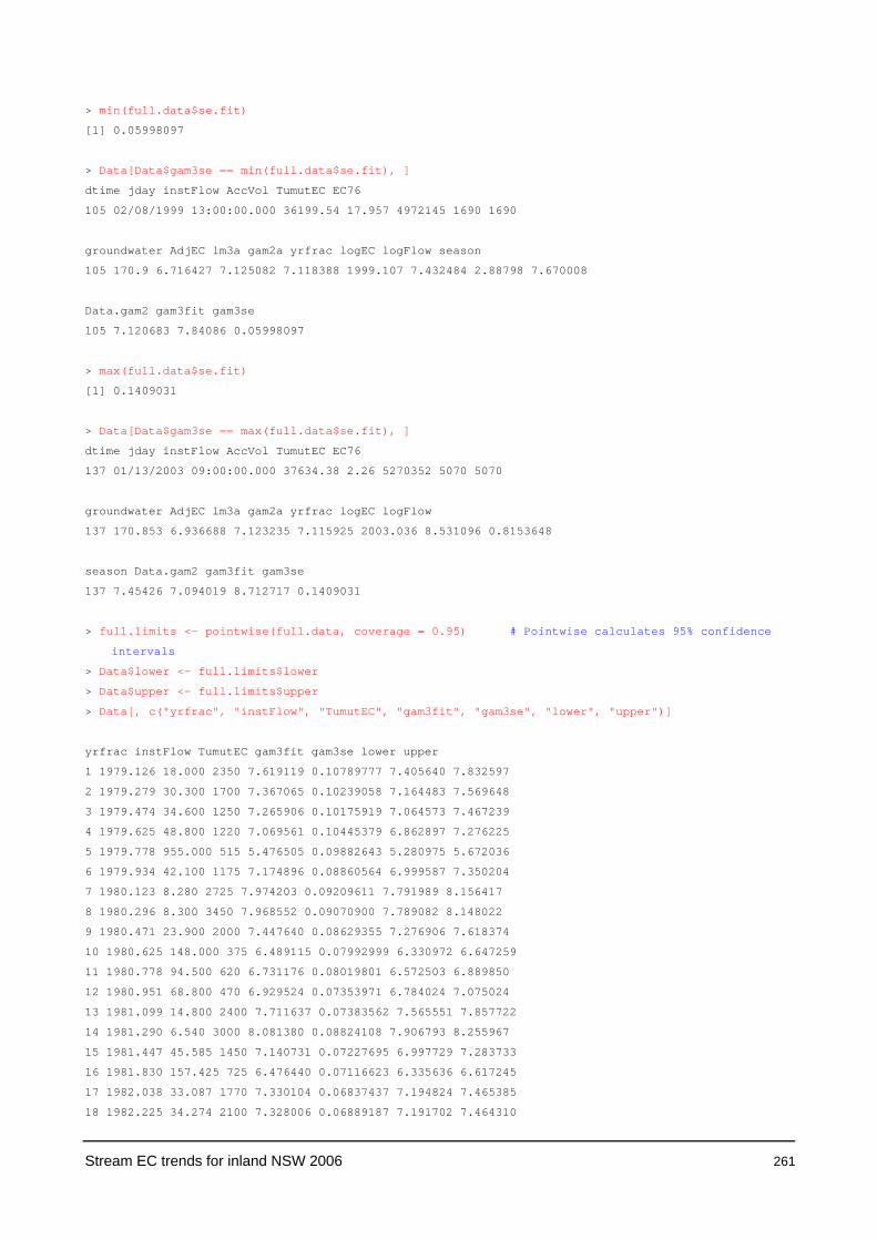
Stream EC trends for inland NSW 2006 261
> min(full.data$se.fit)
[1] 0.05998097
> Data[Data$gam3se == min(full.data$se.fit), ]
dtime jday instFlow AccVol TumutEC EC76
105 02/08/1999 13:00:00.000 36199.54 17.957 4972145 1690 1690
groundwater AdjEC lm3a gam2a yrfrac logEC logFlow season
105 170.9 6.716427 7.125082 7.118388 1999.107 7.432484 2.88798 7.670008
Data.gam2 gam3fit gam3se
105 7.120683 7.84086 0.05998097
> max(full.data$se.fit)
[1] 0.1409031
> Data[Data$gam3se == max(full.data$se.fit), ]
dtime jday instFlow AccVol TumutEC EC76
137 01/13/2003 09:00:00.000 37634.38 2.26 5270352 5070 5070
groundwater AdjEC lm3a gam2a yrfrac logEC logFlow
137 170.853 6.936688 7.123235 7.115925 2003.036 8.531096 0.8153648
season Data.gam2 gam3fit gam3se
137 7.45426 7.094019 8.712717 0.1409031
> full.limits <- pointwise(full.data, coverage = 0.95) # Pointwise calculates 95% confidence
intervals
> Data$lower <- full.limits$lower
> Data$upper <- full.limits$upper
> Data[, c("yrfrac", "instFlow", "TumutEC", "gam3fit", "gam3se", "lower", "upper")]
yrfrac instFlow TumutEC gam3fit gam3se lower upper
1 1979.126 18.000 2350 7.619119 0.10789777 7.405640 7.832597
2 1979.279 30.300 1700 7.367065 0.10239058 7.164483 7.569648
3 1979.474 34.600 1250 7.265906 0.10175919 7.064573 7.467239
4 1979.625 48.800 1220 7.069561 0.10445379 6.862897 7.276225
5 1979.778 955.000 515 5.476505 0.09882643 5.280975 5.672036
6 1979.934 42.100 1175 7.174896 0.08860564 6.999587 7.350204
7 1980.123 8.280 2725 7.974203 0.09209611 7.791989 8.156417
8 1980.296 8.300 3450 7.968552 0.09070900 7.789082 8.148022
9 1980.471 23.900 2000 7.447640 0.08629355 7.276906 7.618374
10 1980.625 148.000 375 6.489115 0.07992999 6.330972 6.647259
11 1980.778 94.500 620 6.731176 0.08019801 6.572503 6.889850
12 1980.951 68.800 470 6.929524 0.07353971 6.784024 7.075024
13 1981.099 14.800 2400 7.711637 0.07383562 7.565551 7.857722
14 1981.290 6.540 3000 8.081380 0.08824108 7.906793 8.255967
15 1981.447 45.585 1450 7.140731 0.07227695 6.997729 7.283733
16 1981.830 157.425 725 6.476440 0.07116623 6.335636 6.617245
17 1982.038 33.087 1770 7.330104 0.06837437 7.194824 7.465385
18 1982.225 34.274 2100 7.328006 0.06889187 7.191702 7.464310

262 Stream EC trends for inland NSW 2006
19 1982.384 31.968 1640 7.343125 0.06919790 7.206215 7.480034
20 1982.556 39.805 1680 7.202753 0.08036520 7.043749 7.361758
21 1982.827 18.095 2200 7.590280 0.09067480 7.410878 7.769682
22 1983.016 5.628 3750 8.160992 0.09633654 7.970388 8.351596
23 1983.184 10.699 1500 7.893272 0.07347576 7.747898 8.038645
yrfrac instFlow TumutEC gam3fit gam3se lower upper
24 1983.362 56.094 620 7.080422 0.06930723 6.943296 7.217549
25 1983.573 1028.000 285 5.479287 0.08352734 5.314026 5.644547
26 1983.822 281.828 595 6.194166 0.07131529 6.053067 6.335265
27 1983.937 146.832 925 6.570944 0.07144003 6.429598 6.712289
28 1984.167 76.427 1060 6.955518 0.07621368 6.804727 7.106308
29 1984.332 77.137 605 6.942043 0.07222603 6.799142 7.084944
30 1984.510 50.578 1515 7.129302 0.07455221 6.981799 7.276805
31 1984.888 106.367 1050 6.755818 0.06974703 6.617822 6.893814
32 1985.126 22.237 2260 7.596883 0.06768951 7.462957 7.730808
33 1985.581 102.700 840 6.776582 0.07304970 6.632052 6.921113
34 1985.775 122.975 880 6.683866 0.07186531 6.541678 6.826053
35 1985.926 96.585 710 6.842225 0.06821334 6.707263 6.977187
36 1986.101 26.892 1500 7.529358 0.06637613 7.398031 7.660685
37 1986.274 14.106 3100 7.838033 0.06924817 7.701023 7.975042
38 1986.425 33.497 1650 7.404613 0.06944363 7.267217 7.542009
39 1986.559 1072.786 170 5.533821 0.08413628 5.367356 5.700287
40 1986.710 1768.319 260 5.254179 0.09194408 5.072266 5.436093
41 1986.885 292.290 683 6.265016 0.07095568 6.124629 6.405404
42 1987.041 89.210 1150 6.936892 0.07049117 6.797424 7.076361
43 1987.208 45.117 1670 7.306930 0.06870375 7.170998 7.442862
44 1987.342 59.595 1550 7.153473 0.06772819 7.019471 7.287475
45 1987.515 182.570 430 6.530991 0.06882430 6.394820 6.667161
46 1987.688 331.784 410 6.193804 0.06883561 6.057611 6.329997
yrfrac instFlow TumutEC gam3fit gam3se lower upper
47 1987.860 81.501 1150 6.968855 0.06817244 6.833974 7.103736
48 1988.036 28.824 1800 7.536319 0.06492144 7.407870 7.664768
49 1988.227 18.974 2740 7.753868 0.06562139 7.624034 7.883701
50 1988.381 65.742 1440 7.120440 0.06754868 6.986793 7.254087
51 1988.559 2759.165 184 5.065924 0.11451616 4.839351 5.292497
52 1988.712 355.432 460 6.180287 0.06928774 6.043200 6.317375
53 1988.860 91.610 1240 6.929898 0.06828601 6.794792 7.065003
54 1989.030 76.530 1000 7.061861 0.06924876 6.924851 7.198872
55 1989.148 26.083 2180 7.622007 0.06634971 7.490733 7.753282
56 1989.337 160.485 760 6.676419 0.07892923 6.520255 6.832582
57 1989.545 537.225 310 5.983613 0.07638041 5.832492 6.134733
58 1989.679 1005.241 222 5.630979 0.08012194 5.472456 5.789502
59 1989.912 279.000 880 6.363327 0.07472370 6.215484 6.511169
60 1990.063 58.306 1630 7.228005 0.07119123 7.087152 7.368859
61 1990.274 40.940 2000 7.416835 0.07146536 7.275439 7.558231
62 1990.485 138.286 834 6.747380 0.07368009 6.601602 6.893158
63 1990.658 2505.000 170 5.148755 0.10901901 4.933058 5.364452
64 1990.830 289.598 710 6.343269 0.07482188 6.195232 6.491306
65 1991.175 52.751 215 7.308282 0.07792153 7.154112 7.462451
66 1991.348 48.001 2125 7.343976 0.07570555 7.194191 7.493762
67 1991.523 143.004 1210 6.740101 0.07822232 6.585336 6.894865

Stream EC trends for inland NSW 2006 263
68 1991.715 1220.000 252 5.561219 0.09089050 5.381390 5.741048
69 1991.868 120.949 1280 6.838856 0.07784214 6.684843 6.992868
yrfrac instFlow TumutEC gam3fit gam3se lower upper
70 1992.058 55.522 1857 7.287082 0.07906743 7.130645 7.443519
71 1995.605 1336.895 253 5.554008 0.09278712 5.370426 5.737589
72 1995.833 183.833 592 6.644267 0.07225298 6.501312 6.787221
73 1995.907 210.449 688 6.585332 0.07390836 6.439102 6.731561
74 1995.964 144.282 879 6.800519 0.07396834 6.654171 6.946867
75 1996.060 94.001 1260 7.045898 0.07581266 6.895901 7.195895
76 1996.216 57.446 1690 7.311876 0.07444257 7.164589 7.459162
77 1996.597 3746.886 127 4.987600 0.12801680 4.734316 5.240885
78 1996.674 395.283 428 6.212827 0.06992153 6.074485 6.351168
79 1996.773 1319.144 228 5.557734 0.08574746 5.388080 5.727387
80 1996.866 183.201 714 6.647355 0.06625399 6.516270 6.778440
81 1996.923 110.414 1190 6.929553 0.06507105 6.800808 7.058298
82 1997.016 111.259 1760 6.943592 0.06958538 6.805915 7.081268
83 1997.093 61.949 1820 7.261654 0.06807079 7.126974 7.396333
84 1997.170 33.202 2380 7.582251 0.06459837 7.454441 7.710060
85 1997.266 30.486 2160 7.619264 0.06393360 7.492770 7.745758
86 1997.342 31.380 2330 7.593348 0.06369345 7.467329 7.719367
87 1997.419 56.095 1730 7.284715 0.06492653 7.156256 7.413173
88 1997.496 53.726 1680 7.289853 0.06755409 7.156196 7.423511
89 1997.822 56.653 1450 7.247117 0.06742489 7.113716 7.380519
90 1997.899 39.554 1740 7.442687 0.06394411 7.316172 7.569202
91 1997.992 16.561 2600 7.880415 0.06461822 7.752566 8.008264
92 1998.090 11.980 3180 8.043944 0.06436844 7.916589 8.171298
yrfrac instFlow TumutEC gam3fit gam3se lower upper
93 1998.148 10.559 3310 8.105323 0.06558905 7.975553 8.235092
94 1998.244 10.454 3490 8.107020 0.06672681 7.974999 8.239041
95 1998.321 26.295 2690 7.666670 0.06159060 7.544811 7.788528
96 1998.397 23.234 2300 7.710570 0.06482080 7.582321 7.838820
97 1998.493 104.536 1271 6.925570 0.06463754 6.797683 7.053457
98 1998.570 51.656 1750 7.278295 0.07107707 7.137668 7.418923
99 1998.647 301.872 323 6.331362 0.06496705 6.202823 6.459901
100 1998.723 202.973 483 6.544774 0.06399342 6.418162 6.671387
101 1998.819 139.077 760 6.756436 0.06221191 6.633349 6.879524
102 1998.877 262.855 895 6.422440 0.06486230 6.294108 6.550771
103 1998.953 35.099 1750 7.494664 0.06030006 7.375358 7.613969
104 1999.030 10.442 2190 8.080386 0.06895098 7.943965 8.216808
105 1999.107 17.957 1690 7.840860 0.05998097 7.722186 7.959534
106 1999.203 14.595 2550 7.939712 0.06195782 7.817127 8.062297
107 1999.279 95.546 649 6.999507 0.07276812 6.855533 7.143480
108 1999.337 24.441 1880 7.681912 0.06207421 7.559097 7.804727
109 2000.430 151.585 606 6.714943 0.06847464 6.579464 6.850422
110 2000.737 504.666 375 6.026490 0.06664022 5.894641 6.158340
111 2000.833 1326.714 168 5.508433 0.08730471 5.335698 5.681167
112 2000.910 208.489 685 6.531955 0.06519072 6.402974 6.660937
113 2000.967 94.104 1330 6.968906 0.06229516 6.845654 7.092159
114 2001.041 51.114 1990 7.299745 0.06155526 7.177956 7.421533
115 2001.118 84.791 1120 7.046607 0.07148097 6.905180 7.188034
yrfrac instFlow TumutEC gam3fit gam3se lower upper

264 Stream EC trends for inland NSW 2006
116 2001.195 27.020 2280 7.629351 0.06221255 7.506262 7.752440
117 2001.271 29.814 2190 7.576212 0.06306605 7.451434 7.700990
118 2001.367 34.685 2120 7.486056 0.06391199 7.359604 7.612507
119 2001.463 145.130 1200 6.722163 0.06839003 6.586852 6.857475
120 2001.521 57.818 1610 7.194550 0.06923530 7.057567 7.331534
121 2001.616 70.505 1620 7.077084 0.07267117 6.933302 7.220866
122 2001.693 118.917 919 6.797646 0.06969949 6.659744 6.935549
123 2001.789 99.154 960 6.899373 0.06820677 6.764424 7.034322
124 2001.885 86.876 828 6.983824 0.06560092 6.854031 7.113617
125 2001.942 29.768 1780 7.540929 0.06683779 7.408689 7.673170
126 2002.038 13.778 2840 7.922678 0.06959783 7.784977 8.060379
127 2002.115 22.611 2850 7.700278 0.06722387 7.567274 7.833282
128 2002.192 18.974 2550 7.785490 0.06933769 7.648303 7.922676
129 2002.288 20.803 2390 7.734172 0.07159256 7.592524 7.875820
130 2002.364 25.554 2370 7.622452 0.07387213 7.476294 7.768610
131 2002.444 19.199 2510 7.740990 0.08181227 7.579122 7.902857
132 2002.518 34.286 1930 7.445185 0.08346400 7.280049 7.610320
133 2002.614 57.676 1180 7.166600 0.08592583 6.996594 7.336606
134 2002.712 29.321 1780 7.501851 0.09549534 7.312911 7.690790
135 2002.770 23.837 1600 7.604956 0.09653518 7.413959 7.795953
136 2002.940 4.511 3840 8.390398 0.11928652 8.154386 8.626409
137 2003.036 2.260 5070 8.712717 0.14090308 8.433937 8.991497
138 2003.189 2.298 5130 8.716846 0.13794577 8.443916 8.989775
> plot(yrfrac, logEC) # plot original data
> abline(h = mean(logEC)) # add a reference line at mean
> title("original log(EC); Blue: gam3; Red: Upper & Lower 95% CI")
> lines(yrfrac, full.data$fit, col = 6, lwd = 4) # add BLUE fitted curve
> lines(yrfrac, full.limits$lower, col = 3, lwd = 2) # add RED lower 95% limits

Stream EC trends for inland NSW 2006 265
> lines(yrfrac, full.limits$upper, col = 3, lwd = 2) # add RED upper 95% limits
yrfrac
logE
C
1980 1985 1990 1995 2000
56
78
original log(EC); Blue: gam3; Red: Upper & Lower 95% CI

266 Stream EC trends for inland NSW 2006
> # ==========================================================================================
# =13=13=13=13=13=13=13=13=13=13=13=13=13=13=13=13=13=13=13=13=13=13=13=13=13=13=13=13=13=13
#===========================================================================================
# Look at impact of including groundwater by comparing these models
#
# 3. Data.gam1 <- gam(logEC ~ s(logFlow,2) + cost + sint)
# 3a D.gam1a <- gam(logEC ~ s(logFlow,2) + cost + sint + s(groundwater,2))
#
# 7. Data.gam3 <- gam(logEC ~ s(logFlow,2) + cost + sint + s(yrfrac, 4))
# 7a D.gam3a <- gam(logEC ~ s(logFlow,2) + cost + sint + s(groundwater, 4)) + s(yrfrac,2)
# ==========================================================================================
> par(mfrow = c(2, 1))
> plot(yrfrac, AdjEC, pch = 16)
> abline(h = mean(logEC))
> lines(lowess(yrfrac, AdjEC), col = 3, lwd = 4)
> title("Adjusted EC; lowess smoother over time")
> plot(groundwater, AdjEC, pch = 16)
> abline(h = mean(logEC))
> lines(lowess(groundwater, AdjEC), col = 3, lwd = 4)
> title("Adjusted EC; lowess smoother over groundwater")
yrfrac
Adj
EC
1980 1985 1990 1995 2000
5.5
6.0
6.5
7.0
7.5
Adjusted EC; lowess smoother over time
groundwater
Adj
EC
166 168 170
5.5
6.0
6.5
7.0
7.5
Adjusted EC; lowess smoother over groundwater

Stream EC trends for inland NSW 2006 267
> # ========== Alternative models =================================================
# 3. Data.gam1 <- gam(logEC ~ s(logFlow,2) + cost + sint)
# 3a D.gam1a <- gam(logEC ~ s(logFlow,2) + cost + sint + s(groundwater,2))
# 7. Data.gam3 <- gam(logEC ~ s(logFlow,2) + cost + sint + s(yrfrac, 4))
# ===============================================================================
> D.gam1a <- gam(logEC ~ s(logFlow, 2) + cost + sint + s(groundwater, 2))
> summary.lm(D.gam1a)
Call: gam(formula = logEC ~ s(logFlow, 2) + cost + sint + s(groundwater, 2))
Residuals:
Min 1Q Median 3Q Max
-1.92 -0.1193 0.0499 0.1817 0.6991
Coefficients:
Value Std. Error t value Pr(>|t|)
(Intercept) 2.4648 2.0171 1.2219 0.2239
s(logFlow, 2) -0.5074 0.0242 -20.9468 0.0000
cost 0.0151 0.0382 0.3964 0.6925
sint 0.0437 0.0473 0.9237 0.3573
s(groundwater, 2) 0.0398 0.0119 3.3393 0.0011
Residual standard error: 0.2988 on 131.001134217726 degrees of freedom
Multiple R-Squared: 0.8617
F-statistic: 210.7 on 4 and 131.001134217726 degrees of freedom, the p-value is 0
Correlation of Coefficients:
(Intercept) s(logFlow, 2) cost sint
s(logFlow, 2) -0.0098
cost 0.0675 0.3308
sint -0.0396 0.6419 0.2282
s(groundwater, 2) -0.9986 -0.0417 -0.0856 0.0062
> summary.lm(D.gam1a, corr = F)
Call: gam(formula = logEC ~ s(logFlow, 2) + cost + sint + s(groundwater, 2))
Residuals:
Min 1Q Median 3Q Max
-1.92 -0.1193 0.0499 0.1817 0.6991
Coefficients:
Value Std. Error t value Pr(>|t|)
(Intercept) 2.4648 2.0171 1.2219 0.2239
s(logFlow, 2) -0.5074 0.0242 -20.9468 0.0000
cost 0.0151 0.0382 0.3964 0.6925
sint 0.0437 0.0473 0.9237 0.3573
s(groundwater, 2) 0.0398 0.0119 3.3393 0.0011
Residual standard error: 0.2988 on 131.001134217726 degrees of freedom
Multiple R-Squared: 0.8617
F-statistic: 210.7 on 4 and 131.001134217726 degrees of freedom, the p-value is 0

268 Stream EC trends for inland NSW 2006
> anova(Data.gam1, D.gam1a)
Analysis of Deviance Table
Response: logEC
Terms Resid. Df Resid. Dev
1 s(logFlow, 2) + cost + sint 133.0002 12.82857
2 s(logFlow, 2) + cost + sint + s(groundwater, 2) 131.0011 11.69496
Test Df Deviance
1
2 +s(groundwater, 2) 1.999023 1.133614
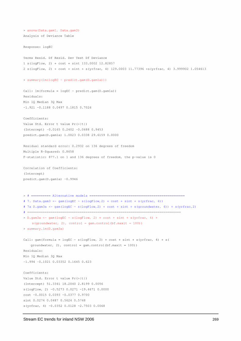
Stream EC trends for inland NSW 2006 269
> anova(Data.gam1, Data.gam3)
Analysis of Deviance Table
Response: logEC
Terms Resid. Df Resid. Dev Test Df Deviance
1 s(logFlow, 2) + cost + sint 133.0002 12.82857
2 s(logFlow, 2) + cost + sint + s(yrfrac, 4) 129.0003 11.77396 +s(yrfrac, 4) 3.999902 1.054613
> summary(lm(logEC ~ predict.gam(D.gam1a)))
Call: lm(formula = logEC ~ predict.gam(D.gam1a))
Residuals:
Min 1Q Median 3Q Max
-1.921 -0.1188 0.0497 0.1815 0.7026
Coefficients:
Value Std. Error t value Pr(>|t|)
(Intercept) -0.0165 0.2402 -0.0688 0.9453
predict.gam(D.gam1a) 1.0023 0.0338 29.6159 0.0000
Residual standard error: 0.2932 on 136 degrees of freedom
Multiple R-Squared: 0.8658
F-statistic: 877.1 on 1 and 136 degrees of freedom, the p-value is 0
Correlation of Coefficients:
(Intercept)
predict.gam(D.gam1a) -0.9946
> # ========== Alternative models =================================================
# 7. Data.gam3 <- gam(logEC ~ s(logFlow,2) + cost + sint + s(yrfrac, 4))
# 7a D.gam3a <- gam(logEC ~ s(logFlow,2) + cost + sint + s(groundwater, 4)) + s(yrfrac,2)
# ===============================================================================
> D.gam3a <- gam(logEC ~ s(logFlow, 2) + cost + sint + s(yrfrac, 4) +
s(groundwater, 2), control = gam.control(bf.maxit = 100))
> summary.lm(D.gam3a)
Call: gam(formula = logEC ~ s(logFlow, 2) + cost + sint + s(yrfrac, 4) + s(
groundwater, 2), control = gam.control(bf.maxit = 100))
Residuals:
Min 1Q Median 3Q Max
-1.994 -0.1021 0.03352 0.1645 0.623
Coefficients:
Value Std. Error t value Pr(>|t|)
(Intercept) 51.3341 18.2040 2.8199 0.0056
s(logFlow, 2) -0.5273 0.0271 -19.4671 0.0000
cost -0.0015 0.0393 -0.0377 0.9700
sint 0.0274 0.0487 0.5624 0.5748
s(yrfrac, 4) -0.0352 0.0128 -2.7503 0.0068
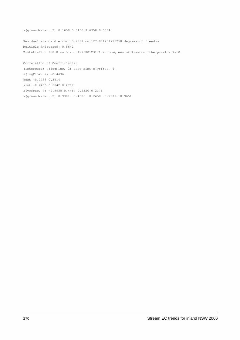
270 Stream EC trends for inland NSW 2006
s(groundwater, 2) 0.1658 0.0456 3.6358 0.0004
Residual standard error: 0.2991 on 127.001231718258 degrees of freedom
Multiple R-Squared: 0.8642
F-statistic: 168.8 on 5 and 127.001231718258 degrees of freedom, the p-value is 0
Correlation of Coefficients:
(Intercept) s(logFlow, 2) cost sint s(yrfrac, 4)
s(logFlow, 2) -0.4436
cost -0.2233 0.3914
sint -0.2406 0.6642 0.2707
s(yrfrac, 4) -0.9938 0.4454 0.2320 0.2378
s(groundwater, 2) 0.9301 -0.4396 -0.2458 -0.2279 -0.9651

Stream EC trends for inland NSW 2006 271
> summary.lm(D.gam3a, corr = F)
Call: gam(formula = logEC ~ s(logFlow, 2) + cost + sint + s(yrfrac, 4) + s(
groundwater, 2), control = gam.control(bf.maxit = 100))
Residuals:
Min 1Q Median 3Q Max
-1.994 -0.1021 0.03352 0.1645 0.623
Coefficients:
Value Std. Error t value Pr(>|t|)
(Intercept) 51.3341 18.2040 2.8199 0.0056
s(logFlow, 2) -0.5273 0.0271 -19.4671 0.0000
cost -0.0015 0.0393 -0.0377 0.9700
sint 0.0274 0.0487 0.5624 0.5748
s(yrfrac, 4) -0.0352 0.0128 -2.7503 0.0068
s(groundwater, 2) 0.1658 0.0456 3.6358 0.0004
Residual standard error: 0.2991 on 127.001231718258 degrees of freedom
Multiple R-Squared: 0.8642
F-statistic: 168.8 on 5 and 127.001231718258 degrees of freedom, the p-value is 0
> anova(Data.gam3, D.gam3a)
Analysis of Deviance Table
Response: logEC
Terms Resid. Df
1 s(logFlow, 2) + cost + sint + s(yrfrac, 4) 129.0003
2 s(logFlow, 2) + cost + sint + s(yrfrac, 4) + s(groundwater, 2) 127.0012
Resid. Dev Test Df Deviance
1 11.77396
2 11.36316 +s(groundwater, 2) 1.999023 0.4108005
> summary(lm(logEC ~ predict.gam(D.gam3a)))
Call: lm(formula = logEC ~ predict.gam(D.gam3a))
Residuals:
Min 1Q Median 3Q Max
-1.995 -0.1009 0.03245 0.1641 0.6274
Coefficients:
Value Std. Error t value Pr(>|t|)
(Intercept) -0.0217 0.2364 -0.0919 0.9269
predict.gam(D.gam3a) 1.0031 0.0333 30.1116 0.0000
Residual standard error: 0.289 on 136 degrees of freedom
Multiple R-Squared: 0.8696
F-statistic: 906.7 on 1 and 136 degrees of freedom, the p-value is 0
Correlation of Coefficients:

272 Stream EC trends for inland NSW 2006
(Intercept)
predict.gam(D.gam3a) -0.9946
> AIC(Data.lm1, Data.lm2, Data.gam1, D.gam1a, Data.gam3, D.gam3a)
df AIC
Data.lm1 3 75.17125
Data.lm2 5 77.88274
Data.gam1 5 73.79718
D.gam1a 6 63.02983
Data.gam3 6 63.95890
D.gam3a 7 61.05800

Stream EC trends for inland NSW 2006 273
Appendix 8—Derivation of {100 × (eη – 1)}
The linear coefficient of time, η, was used to calculate the percentage change in EC per annum using the formula {100 × (eη – 1)}. Derivation of this formula is now presented.
For simplicity, we can ignore terms in our model such as logeflow and the seasonality sin and cos terms. Doing this, the form of the equation we are fitting is:
loge(EC) = a + b·time + error,
but for ease of manipulation, let us write it as
loge(Y) = a + b·X,
which can be represented on the natural Y scale by
Y = exp{a + b·X}.
Let’s make up an example data set using a = 0.5 and b = 0.2; that is, Y = exp(0.5 + 0.2X). On the natural Y scale, the relationship is curvilinear (left graph), and on the loge(Y) scale, the relationship is linear (right graph).
Looking at this curve (enlarged for clarity below), we note the change in Y per unit of X, which, when using the 5th and 6th values, is an additional (5.474 – 4.482 =) 0.992 units of Y per unit of X. This amount will, of course, change with various selections of X values (seen in the table below). However, the proportional change does not vary; that is, 0.992 units change as a proportion of its ‘starting value’ of 4.482 is a 0.221 proportional increase.
X Data
0 2 4 6 8 10 12
Y D
ata
0
2
4
6
8
10
12
14
X Data
0 2 4 6 8 10 12
log e(
Y D
ata)
e0
e1
e2
e3
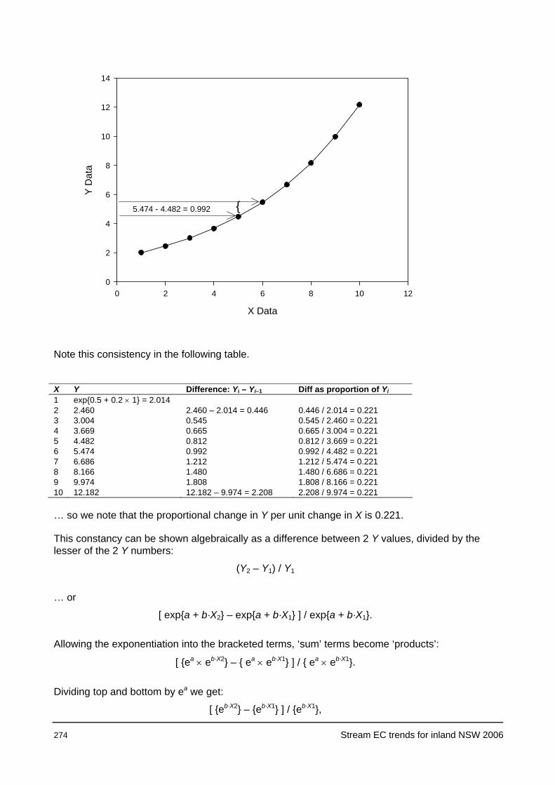
274 Stream EC trends for inland NSW 2006
Note this consistency in the following table.
X Y Difference: Yi – Yi–1 Diff as proportion of Yi 1 exp{0.5 + 0.2 × 1} = 2.014 2 2.460 2.460 – 2.014 = 0.446 0.446 / 2.014 = 0.221 3 3.004 0.545 0.545 / 2.460 = 0.221 4 3.669 0.665 0.665 / 3.004 = 0.221 5 4.482 0.812 0.812 / 3.669 = 0.221 6 5.474 0.992 0.992 / 4.482 = 0.221 7 6.686 1.212 1.212 / 5.474 = 0.221 8 8.166 1.480 1.480 / 6.686 = 0.221 9 9.974 1.808 1.808 / 8.166 = 0.221 10 12.182 12.182 – 9.974 = 2.208 2.208 / 9.974 = 0.221
… so we note that the proportional change in Y per unit change in X is 0.221.
This constancy can be shown algebraically as a difference between 2 Y values, divided by the lesser of the 2 Y numbers:
(Y2 – Y1) / Y1
… or
[ exp{a + b·X2} – exp{a + b·X1} ] / exp{a + b·X1}.
Allowing the exponentiation into the bracketed terms, ‘sum’ terms become ‘products’:
[ {ea × eb·X2} – { ea × eb·X1} ] / { ea × eb·X1}.
Dividing top and bottom by ea we get:
[ {eb·X2} – {eb·X1} ] / {eb·X1},
X Data
0 2 4 6 8 10 12
Y D
ata
0
2
4
6
8
10
12
14
5.474 - 4.482 = 0.992 {

Stream EC trends for inland NSW 2006 275
and then dividing top and bottom by eb·X1 we get (when dividing terms with exponents, division becomes difference):
[ eb·X2 – b·X1 – 1 ],
which equals:
[ eb (X2 – X1) – 1 ].
Since X2 – X1 is unity, this can be rewritten as:
[ eb – 1 ].
Since for this example b = 0.2, then we note:
[ e0.2 – 1 ] = 0.221.
So the proportional change in Y per unit of X is (eη – 1), and the percentage change in Y per unit of X is {100 × (eη – 1)}.


Stream EC trends for inland NSW 2006 277
Annexure A—Aspects of Archived Electrical Conductivity Data in TRITON
By F. J. Harvey
Acknowledgments
Rodger Grayson, who provided advice on the various drafts. Terry Koen and Sarah McGeoch, who proof-read and edited this document and provided advice. The staff of the Armidale and Tumut hydrographic offices who assisted in the data evaluation. Department of Environment and Climate Change NSW Wagga Wagga Research Centre March 2006

278 Stream EC trends for inland NSW 2006
Contents
Abstract .............................................................................................................................. 280
1 Introduction................................................................................................................... 281
2 TRITON Archive—Historical EC 1960s to 1992........................................................... 282 2.1 Southern districts record ................................................................................ 282 2.2 Northern districts record................................................................................. 284
3 TRITON Archive After 1992 ......................................................................................... 291
4 Historical Data Discussion............................................................................................ 292 4.1 Origins of the discrepancy.............................................................................. 292 4.2 Options for EC trend analyses ....................................................................... 292 4.3 Ramifications of data adjustment—sensitivity tests ....................................... 293 4.4 Resolving the bias.......................................................................................... 295
5 Conclusion.................................................................................................................... 297
6 References ................................................................................................................... 297

Stream EC trends for inland NSW 2006 279
Figures
Figure 1a. Correction (μS/cm) to Tumut data using laboratory analyses as datum. .......... 283
Figure 1b. Correction (percentage) to Tumut data using laboratory analyses as datum. .. 284
Figure 2a. Correction (μS/cm) to Armidale data using laboratory analyses as datum. ...... 285
Figure 2b. Correction (percentage) to Armidale data using laboratory analyses as datum.286
Figure 3. Correction (percentage) to Armidale data using laboratory analyses as datum. 287
Tables
Table 1. Southern sites exhibiting no change in sign of trend............................................ 294
Table 2. Southern sites exhibiting change in sign of trend................................................. 294
Table 3. Northern sites exhibiting no change in sign of trend. ........................................... 295
Table 4. Northern sites exhibiting change in sign of trend. ................................................ 295

280 Stream EC trends for inland NSW 2006
Abstract
This report is an annexure to ‘2006 Stream EC Trends for Inland NSW ’. One of the first steps in this investigation was an examination of the data. Most of the electrical conductivity (EC) data was obtained from the Department of Water and Energy’s (DWE) TRITON database.
This report investigates data sources in the northern and southern parts of NSW. It flags a potential major anomaly in the TRITON archive and describes how it was handled in ‘2006 Stream EC Trends for Inland NSW’. The anomaly took the form of a possible systematic error in the earlier data record. The implications for trend analysis are discussed. The report also flags a number of other minor issues that will need to be addressed by the archive manager.

Stream EC trends for inland NSW 2006 281
1 Introduction
As a prelude to the stream EC trends investigation, a review was undertaken of the EC data collected during (regular) visits to water quality monitoring sites. Here, these data are termed ‘discrete data’. The TRITON database holds most of this data and its ancillary information. The data investigation revealed a number of issues with profound implications for the way that this EC data is (and has previously been) used in trend analysis.
The grab-sampling programs that generated the discrete data have been considered in two blocks. The first block was operated by hydrographic staff from the late 1960s to the early 1990s and is termed ’historical’ here. At most sites, there is a second block of data (starting in the early 1990s). This second block was mostly (but not always) generated under the one collection program.

282 Stream EC trends for inland NSW 2006
2 TRITON Archive—Historical EC 1960s to 1992
EC meters were used in the Tumut and Armidale offices to measure the grab samples taken in the field by departmental hydrographic teams. The sampling program was in its infancy and required a checking procedure of the Tumut/Armidale instruments – sometimes duplicate samples were sent to Sydney for laboratory analysis. Gauging stations used in the data checking procedure are listed in old records at the Armidale and Tumut offices. The dates (before the early 1990s) when the comparisons occurred can usually be identified in TRITON because they contain two different EC readings.
The exercise of separating the 2 data strands (Armidale/Tumut and laboratory data) has led to the conclusion that a bias exists in the historical dataset before 1992. The apparent bias has implications for the comparison of EC trends at different sites.
2.1 Southern districts record
Most of the historical EC data from the Murray, Murrumbidgee and Lachlan valleys was measured in the Tumut office. The TRITON archive is ambiguous on this fact, describing all the early data under a ‘Laboratory Codes’ heading as ‘unknown / not recorded’. This labelling is misleading, as it is open to an interpretation that the data were analysed under accredited laboratory conditions, but that the details have been lost. However, this investigation has found that the data was not analysed under accredited laboratory conditions, and the source (Tumut office) is known.
As most historical readings can be traced back to Tumut, the TRITON database could be vastly improved by creating a specific code for the Tumut (and Armidale) EC meters. Such a step would clarify a large proportion of the samples currently labelled as ‘unknown’.
2.1.1 Tumut sampling program
In the historical program, grab samples were obtained during site visits and brought back to Tumut to be measured. They were then processed in batches, and the results were recorded there. In some instances, duplicate samples were sent to Sydney for laboratory analysis for the purpose of checking the Tumut meter. Of the sites selected as suitable for the stream EC trend study, only a few were part of the historical checking. The TRITON record suggests that gauging station 401009 Maragle Creek at Maragle was the subject of an extensive checking program. This study identified 5 other stations with occasional duplicate readings—410061 Adelong Creek at Batlow Road, 401013 Jingellic Creek at Jingellic, 410044 Muttama Creek at Coolac, 410047 Tarcutta Creek at Old Borambola and 410048 Kyeamba Creek at Ladysmith. A cursory investigation suggests that there are other duplicate sites, but these were not listed for inclusion in the EC trend study, and there were no additional resources to invest in the data editing.
By comparing the TRITON archive with the results held at Tumut, it is possible to isolate the Tumut readings. It was assumed that the remainder were Sydney laboratory readings. After editing for gross errors, the performance of the Tumut EC meter can be compared with the Sydney laboratory (Figures 1a, b). These figures are based on the premise that the laboratory results are correct (time constraints prevented confirmation of this).
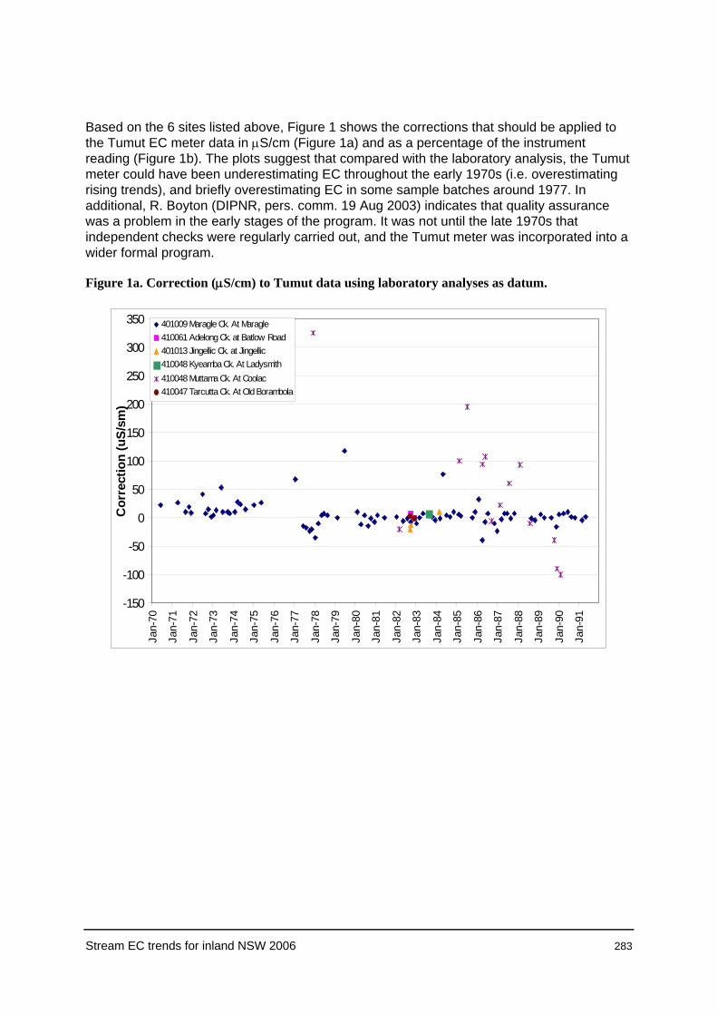
Stream EC trends for inland NSW 2006 283
Based on the 6 sites listed above, Figure 1 shows the corrections that should be applied to the Tumut EC meter data in μS/cm (Figure 1a) and as a percentage of the instrument reading (Figure 1b). The plots suggest that compared with the laboratory analysis, the Tumut meter could have been underestimating EC throughout the early 1970s (i.e. overestimating rising trends), and briefly overestimating EC in some sample batches around 1977. In additional, R. Boyton (DIPNR, pers. comm. 19 Aug 2003) indicates that quality assurance was a problem in the early stages of the program. It was not until the late 1970s that independent checks were regularly carried out, and the Tumut meter was incorporated into a wider formal program.
Figure 1a. Correction (μS/cm) to Tumut data using laboratory analyses as datum.
-150
-100
-50
0
50
100
150
200
250
300
350
Jan-
70
Jan-
71
Jan-
72
Jan-
73
Jan-
74
Jan-
75
Jan-
76
Jan-
77
Jan-
78
Jan-
79
Jan-
80
Jan-
81
Jan-
82
Jan-
83
Jan-
84
Jan-
85
Jan-
86
Jan-
87
Jan-
88
Jan-
89
Jan-
90
Jan-
91
Cor
rect
ion
(uS/
sm)
401009 Maragle Ck. At Maragle410061 Adelong Ck. at Batlow Road401013 Jingellic Ck. at Jingellic410048 Kyeamba Ck. At Ladysmith410048 Muttama Ck. At Coolac410047 Tarcutta Ck. At Old Borambola
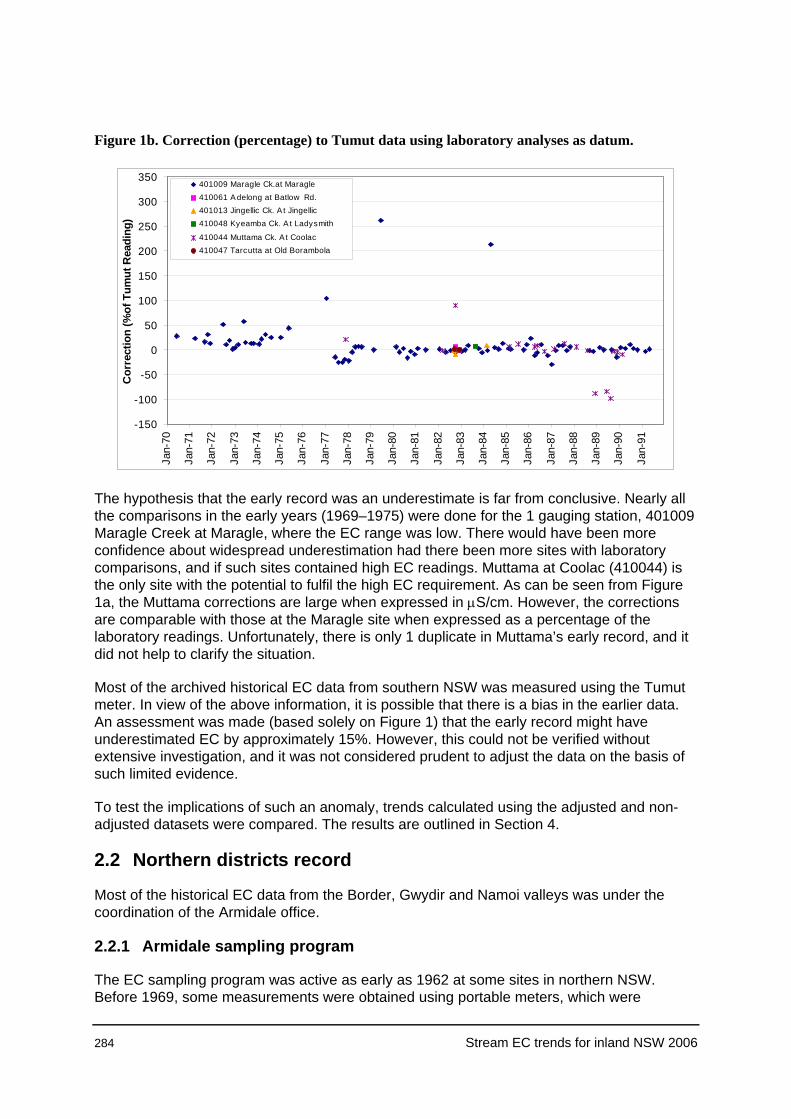
284 Stream EC trends for inland NSW 2006
Figure 1b. Correction (percentage) to Tumut data using laboratory analyses as datum.
-150
-100
-50
0
50
100
150
200
250
300
350Ja
n-70
Jan-
71
Jan-
72
Jan-
73
Jan-
74
Jan-
75
Jan-
76
Jan-
77
Jan-
78
Jan-
79
Jan-
80
Jan-
81
Jan-
82
Jan-
83
Jan-
84
Jan-
85
Jan-
86
Jan-
87
Jan-
88
Jan-
89
Jan-
90
Jan-
91
Cor
rect
ion
(%of
Tum
ut R
eadi
ng)
401009 Maragle Ck.at Maragle410061 A delong at Batlow Rd.401013 Jingellic Ck. A t Jingellic410048 Kyeamba Ck. A t Ladysmith
410044 Muttama Ck. A t Coolac410047 Tarcutta at Old Borambola
The hypothesis that the early record was an underestimate is far from conclusive. Nearly all the comparisons in the early years (1969–1975) were done for the 1 gauging station, 401009 Maragle Creek at Maragle, where the EC range was low. There would have been more confidence about widespread underestimation had there been more sites with laboratory comparisons, and if such sites contained high EC readings. Muttama at Coolac (410044) is the only site with the potential to fulfil the high EC requirement. As can be seen from Figure 1a, the Muttama corrections are large when expressed in μS/cm. However, the corrections are comparable with those at the Maragle site when expressed as a percentage of the laboratory readings. Unfortunately, there is only 1 duplicate in Muttama’s early record, and it did not help to clarify the situation.
Most of the archived historical EC data from southern NSW was measured using the Tumut meter. In view of the above information, it is possible that there is a bias in the earlier data. An assessment was made (based solely on Figure 1) that the early record might have underestimated EC by approximately 15%. However, this could not be verified without extensive investigation, and it was not considered prudent to adjust the data on the basis of such limited evidence.
To test the implications of such an anomaly, trends calculated using the adjusted and non-adjusted datasets were compared. The results are outlined in Section 4.
2.2 Northern districts record
Most of the historical EC data from the Border, Gwydir and Namoi valleys was under the coordination of the Armidale office.
2.2.1 Armidale sampling program
The EC sampling program was active as early as 1962 at some sites in northern NSW. Before 1969, some measurements were obtained using portable meters, which were
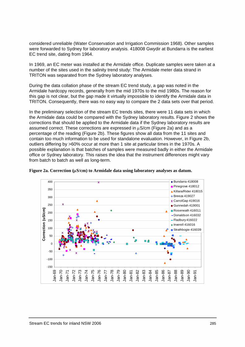
Stream EC trends for inland NSW 2006 285
considered unreliable (Water Conservation and Irrigation Commission 1968). Other samples were forwarded to Sydney for laboratory analysis. 418008 Gwydir at Bundarra is the earliest EC trend site, dating from 1964.
In 1969, an EC meter was installed at the Armidale office. Duplicate samples were taken at a number of the sites used in the salinity trend study: The Armidale meter data strand in TRITON was separated from the Sydney laboratory analyses.
During the data collation phase of the stream EC trend study, a gap was noted in the Armidale hardcopy records, generally from the mid 1970s to the mid 1980s. The reason for this gap is not clear, but the gap made it virtually impossible to identify the Armidale data in TRITON. Consequently, there was no easy way to compare the 2 data sets over that period.
In the preliminary selection of the stream EC trends sites, there were 11 data sets in which the Armidale data could be compared with the Sydney laboratory results. Figure 2 shows the corrections that should be applied to the Armidale data if the Sydney laboratory results are assumed correct. These corrections are expressed in μS/cm (Figure 2a) and as a percentage of the reading (Figure 2b). These figures show all data from the 11 sites and contain too much information to be used for standalone evaluation. However, in Figure 2b, outliers differing by >60% occur at more than 1 site at particular times in the 1970s. A possible explanation is that batches of samples were measured badly in either the Armidale office or Sydney laboratory. This raises the idea that the instrument differences might vary from batch to batch as well as long-term.
Figure 2a. Correction (μS/cm) to Armidale data using laboratory analyses as datum.
-150
-100
-50
0
50
100
150
200
250
300
350
400
Jan-
69Ja
n-70
Jan-
71Ja
n-72
Jan-
73Ja
n-74
Jan-
75Ja
n-76
Jan-
77Ja
n-78
Jan-
79Ja
n-80
Jan-
81Ja
n-82
Jan-
83Ja
n-84
Jan-
85Ja
n-86
Jan-
87Ja
n-88
Jan-
89Ja
n-90
Jan-
91
Cor
rect
ion
(uS/
cm)
Bundarra 418008Pinegrove 418012Killara/Rider 418015Breeza 419027CarrolGap 419016Gunnedah 419001Roseneath 416011Donaldson 416032Fladbury 416022Inverell 416016Strathbogie 416039
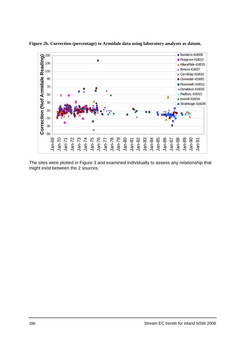
286 Stream EC trends for inland NSW 2006
Figure 2b. Correction (percentage) to Armidale data using laboratory analyses as datum.
-50
-30
-10
10
30
50
70
90
110
130
150Ja
n-69
Jan-
70Ja
n-71
Jan-
72Ja
n-73
Jan-
74Ja
n-75
Jan-
76Ja
n-77
Jan-
78Ja
n-79
Jan-
80Ja
n-81
Jan-
82Ja
n-83
Jan-
84Ja
n-85
Jan-
86Ja
n-87
Jan-
88Ja
n-89
Jan-
90Ja
n-91
Cor
rect
ion
(%of
Arm
idal
e R
eadi
ng) Bundarra 418008
Pinegrove 418012Killara/Ride 418015Breeza 419027CarrolGap 419016Gunnedah 419001Roseneath 416011Donaldson 416032Fladbury 416022Inverell 416016Strathbogie 416039
The sites were plotted in Figure 3 and examined individually to assess any relationship that might exist between the 2 sources.

Stream
EC
trends for inland NS
W 2006
287
Figure 3. Correction (percentage) to Armidale data using laboratory analyses as datum.
416011 Dumaresq at Roseneath
-30
-20
-10
0
10
20
30
40
50
60
70
Jun-68 Mar-71 Dec-73 Aug-76 May-79 Feb-82 Nov-84 Aug-87 May-90
Date
Cor
rn. (
%of
Arm
idal
e R
eadi
ng)
416027 Severn R. at Fladbury
-20-15-10
-505
10152025
Jun-68 Dec-73 May-79 Nov-84 May-90 Oct-95
Date
Cor
rn. (
%of
Arm
idal
e re
adin
g)
416016 Macintyre R. at Inverell
0
10
20
30
40
50
60
Jun-68 Mar-71 Dec-73 Aug-76 May-79 Feb-82 Nov-84
Date
Cor
rn. (
%of
Arm
idal
e R
eadi
ng)
416032 Mole R. at Donaldson
-60
-40
-20
0
20
40
60
80
Jun-68 Dec-73 May-79 Nov-84 May-90
Date
Cor
rn. (
%of
Arm
idal
e R
eadi
ng)

288 S
tream E
C trends for inland N
SW
2006
418012 Gwydir R. at Pinegrove
-30
-20-10
010
2030
4050
60
Jun-68 Oct-69 Mar-71 Jul-72 Dec-73 Apr-75 Aug-76
Date
Cor
rn. (
%of
Arm
idal
e re
adin
g)
416039 Severn R. at Strathbogie
-20
-15
-10
-50
5
10
15
20
Jun-68 Dec-73 May-79 Nov-84 May-90
Date
Cor
rn. (
%of
Arm
idal
e re
adin
g)
418008 Gwydir R. at Bundarra
-20
0
20
40
60
80
100
120
140
160
Jun-68 Mar-71 Dec-73 Aug-76 May-79 Feb-82 Nov-84 Aug-87
Date
Cor
rn. (
%of
Arm
idal
e R
eadi
ng)
418015 Horton R. at Killara
-20-10
01020304050607080
Jun-68 Dec-73 May-79 Nov-84 May-90 Oct-95Date
Cor
rn. (
%of
Arm
idal
e R
eadi
ng)
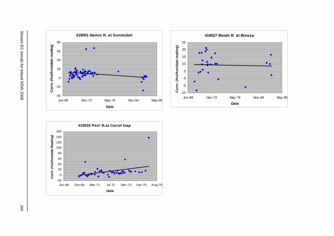
Stream
EC
trends for inland NS
W 2006
289
419001 Namoi R. at Gunnedah
-40
-20
0
20
40
60
80
Jun-68 Dec-73 May-79 Nov-84 May-90
Date
Cor
rn. (
%of
Arm
idal
e re
adin
g)
419027 Mooki R. at Breeza
-10
-5
0
5
10
15
20
25
Jun-68 Dec-73 May-79 Nov-84 May-90
Date
Cor
rn. (
%of
Arm
idal
e re
adin
g)
419016 Peel R.at Carrol Gap
-20
0
20
40
60
80
100
120
140
160
Jun-68 Oct-69 Mar-71 Jul-72 Dec-73 Apr-75 Aug-76
Date
Cor
rn. (
%of
Arm
idal
e R
eadi
ng)

290 Stream EC trends for inland NSW 2006
The information in Figure 3 was assessed by eye, and the ramifications of this approach are discussed in Section 4.
It was concluded that the Armidale EC meter was reading approximately 10% lower than the Sydney laboratory results from 1969. The gap in the Armidale hardcopy records made it difficult to finalise how long the situation continued. The 10% discrepancy could be definitely tracked to the end of 1977, and possibly extended to October 1980. The available information suggests that the data from the 2 measuring systems had achieved reasonable agreement by late 1986, and possibly as early as December 1984.
We concluded that a discrepancy of the order of 10% exists in Triton for the Armidale data until at least the end of 1977. The datasets used to draw this conclusion came from the sites used in the stream EC trend analysis study. They represent about half of the data sets that should have been prepared and analysed for an accurate calculation of the adjustment, but time constraints prevented a thorough analysis. The 10% value was considered a reasonable approximation.

Stream EC trends for inland NSW 2006 291
3 TRITON Archive after 1992
From 1992, the hydrographic staff ceased to be the main data collectors, and a number of different programs evolved for data collection. During the preparation of the TRITON data sets for this study, several issues became apparent:
Laboratory staff apply code ‘NEWVER’ in TRITON after analysis but before final clearance. The code flags that the data point has not been validated. There seems to be some confusion as to who is responsible for the final approval.
At a few sites, good-quality EC data were being collected but without instantaneous flow data. These sites could not be used in the stream EC trend study, because the analysis methods rely on flow-weighting of the EC data. Accurate temperature data are also necessary in EC field sampling.
If there is more than 1 reading during a site visit, the additional information should add to our knowledge of EC behaviour. In the stream EC trend study, variations in the data need to be explained in the context of the flow variations across the stream. Perhaps TRITON requires an EC cross-section archiving procedure similar to Step 2 of DWE Hydrometric Procedure 73044.
If portable meters are used to measure field data, then instrument performance must be tracked over long periods. In TRITON, the portable meters measurements often differ from the laboratory analyses. The portable meter data in TRITON should be flagged as unedited.
Any procedure which condones the frequent undocumented adjustment of a portable EC meter in the field is flawed, because the adjustment masks other sources of failures in the process.
EC data from the Murrumbidgee Valley are stored under 2 variables in TRITON: ‘EC @ 25’ and ‘EC’. Both variables should be downloaded in order to recover all the data.

292 Stream EC trends for inland NSW 2006
4 Historical Data Discussion
Discrepancies between Tumut data / Armidale data and laboratory data need evaluation. At many sites (particularly in southern NSW), the Tumut meter readings are the only available data. If it is concluded that the local procedures were flawed in the early years, then the trend analyses for many sites across the State contain a bias.
4.1 Origins of the discrepancy
Intuitively, we might expect that the local meters are the source of the error. However, it is quite possible that the laboratory results are the source, because the differences are of the same order in Armidale and Tumut. The laboratory analyses have been assessed visually in Microsoft Excel and are generally around 10% to 15% higher than the 2 local meter readings. It is possible that the differences could be explained by either the sample handling or the laboratory analysis.
Handling. It is not clear what time elapsed between sampling and analysis. It is possible that up to a week passed between sampling and return to Tumut or Armidale. R. Boyton (DIPNR, pers. comm. 2004) indicated that:
not many samples were sent from Tumut to Sydney for analysis
most of those sent from Tumut were chilled—e.g. 401009 Maragle Creek at Maragle
if samples were no longer chilled on arrival, they were not used for laboratory analysis.
Various informal discussions at the Armidale and Tumut offices implied some concern about the delays in samples sent to Sydney by rail. It is unlikely that the delays had any effect on the samples because of the static nature of salt.
Laboratory procedures. If the discrepancies were a result of laboratory procedures or equipment, then they should be similar between Tumut and Armidale. Indeed, there was a 15% variation in Tumut data and 10% in Armidale data. However, the hypothesis is weakened by the fact that the Tumut discrepancy alters drastically in 1977 and then disappears shortly thereafter. In comparison, the Armidale discrepancy remains unaltered throughout 1977, and appears to continue throughout 1978.
Quality assurance. Informal enquiries suggest that the Sydney laboratory may not have had QA in the early record.
4.2 Options for EC trend analyses
To progress, we need to identify the source of the error. There are 3 possibilities:
The laboratory readings are correct, and the EC meters are out by 10% in Armidale and 15% in Tumut.
The EC meter results are more or less correct, and the laboratory procedures, instrumentation or sample delivery created an error of >10%.
All the sources contribute to the error in roughly equal proportions.
A solution might have been to average the 2 data sets, but as most of the southern sites didn’t have laboratory check readings, this was not an option. It was concluded that there was no way of apportioning the discrepancy without local knowledge. Informal inquiries indicated that a definitive answer might be elusive at this late date, and would probably require extensive investigations.

Stream EC trends for inland NSW 2006 293
As a short-term solution, it was decided to undertake a sensitivity analysis, using the local and laboratory data to generate 2 EC trends at each site. This would reveal whether the data differences had a major impact on the trend results and could explain the trends ascribed to certain sites in previous studies.
The data sets were generated in the following way for each gauging station. Where duplicates were found, the local readings were identified first, and the remainder were attributed laboratory status. Where there was only the local source, the early records were adjusted: by +15% for Tumut data before 1976 (the overestimates during 1977 were ignored) and by +10% for Armidale data before 1978.
4.3 Ramifications of data adjustment—sensitivity tests
How the bias is corrected may determine whether the EC trend at any particular site is rising or not. The early data bias had far-reaching implications. It was decided to run a sensitivity test, analysing adjusted and unadjusted data using the methods described in Harvey et al. (2009).
4.3.1 Southern NSW
A sensitivity analysis was undertaken to see the effect of the adjustment on the (loge) linear component of the EC trend in the Lachlan, Murrumbidgee and Murray valleys. At the 23 sites where a comparison could be made, the slope always decreased (i.e. became more negative), but the outcomes were not always statistically significant. It was decided to use the existing archive data, although it was suspected that the EC in the earlier years should be increased by approximately 15%.
At 18 of the southern sites, there was no change in the sign of the slope (Table 1). Of these:
7 slopes were already negative and became statistically significant
8 remained positive and statistically significant
3 remained positive but became statistically non-significant.

294 Stream EC trends for inland NSW 2006
Table 1. Southern sites exhibiting no change in sign of trend.
StationNo. NameLinear Trend
Sign Statistical Significance401013 Jingellic Ck. at Jingellic Negative Becomes Significant410091 Billabong Ck. at Walbundrie Positive Significant410097 Billabong Ck. at Aberfeldy Positive Significant410025 Jugiong Ck. at Jugiong Positive Significant410038 Adjungbilly Ck. at Darbalara Negative Becomes Significant410044 Muttama Ck. at Coolac Positive Significant410045 Billabung Ck. at Sunnyside Positive Not Significant410047 Tarcutta Ck. at Old Borambola Positive Significant410048 Kyeamba Ck. at Ladysmith Positive Significant410061 Adelong Ck. at Batlow Rd. Negative Becomes Significant410103 Houlaghans Ck. at Downside Positive Significant412028 Abercrombie R. at Abercrombie Negative Becomes Significant412030 Mandagery Ck.at U/S Eugowra Positive Significant412050 Crookwell R. at Narrawa North Negative Becomes Significant412065 Lachlan R. at Narrawa Positive Becomes Not Significant412072 Back Ck at Koorawatha Positive Becomes Not Significant412083 Tuena Ck. at Tuena Negative Becomes Significant412086 Goobang Ck. at Parkes Negative Becomes Significant
At the 5 remaining southern sites (Table 2), the adjustment would have changed the slope of the trend from positive to negative, but the slopes were statistically non-significant.
Table 2. Southern sites exhibiting change in sign of trend.
StationNo. Name Linear Trend Sign Statistical Significance401009 Maragle at Maragle Becomes Negative Not Significant410057 Goobragandra at Lacmalac Becomes Negative Not Significant412009 Belubula at Canowindra Becomes Negative Becomes Not Signific412043 Goobang at DarbysDam Becomes Negative Becomes Not Signific412055 Belubula at Bangaroo Bge Becomes Negative Not Significant
4.3.2 Northern NSW
In the Macintyre, Gwydir and Namoi, the existing archive data was adjusted by +10% in the earlier record. It was suspected that the real difference might be several percentage points higher. A sensitivity analysis was undertaken to see the effect of the adjustment on the slope of the EC trend. At the 30 sites where a comparison could be made, the slope always reduced in magnitude, becoming relatively more negative, but the outcomes were not always statistically significant.
The sign of the trend slope did not change at 18 sites (Table 3):
4 slopes remained negative and significant
3 remained negative and non-significant
4 remained negative but became statistically significant
1 remained positive and significant
3 remained positive and non-significant

Stream EC trends for inland NSW 2006 295
3 remained positive but became non-significant.
Table 3. Northern sites exhibiting no change in sign of trend.
StationNo. Name
Linear Trend Sign Statistical Significance
416008 Beardy at Haystack Negative Significant416010 Macintyre at Wallangra Negative Not Significant416020 Ottleys at Coolatai Positive Not Significant416027 GilGil at Weemelah Positive Not Significant417001 Moonie at Gundablouie Positive Not Significant418005 CopesCk. At Kimberley Negative Becomes Significant418014 Gwydir at Yarrowych Negative Becomes Significant418021 Laura at Laura Positive Becomes Not Signific.418023 Moredun at Bundarra Positive Becomes Not Signific.418025 Halls at Bingara Negative Significant418027 Horton at DamSite Negative Significant418029 Gwydir at StoneyBatter Positive Becomes Not Signific.419005 Namoi at NthCuerindi Negative Becomes Significant419016 Cockburn at Mulla Xing Negative Significant419027 Mooki at Breeza Positive Significant419029 Halls Ck. At Ukalon Negative Becomes Significant419032 Coxs at Boggabri Negative Not Significant419054 Swamp Ck. At Limbri Negative Not Significant
In northern NSW, the adjustment resulted in 12 sites changing slope from positive to negative (Table 4). None of the slopes, either before or after the adjustment, was statistically significant.
As can be seen, the impact of the data adjustments is not dramatic in the statistical sense. However, the linear trend changed sign (from positive negative) at 17 of the study sites (Tables 2 and 4). Such a change would influence an observer’s perception of the processes. It also adds a layer of uncertainty in forecasting EC levels.
Table 4. Northern sites exhibiting change in sign of trend.
StationNo. Name Linear Trend Sign Statistical Significance416003 Tenterfield at Clifton Becomes Negative Not Significant416016 Macintyre at Inverell Becomes Negative Not Significant416023 Deepwater at Bolivia Becomes Negative Not Significant418015 Horton at Rider Becomes Negative Not Significant418016 Warialda at Warialda Becomes Negative Not Significant418017 Myall at Molroy with 4/1980 Becomes Negative Not Significant418018 Keera at Keera Becomes Negative Not Significant418032 Tycannah at Horseshoe Becomes Negative Not Significant419033 Coxs at Tambar springs Becomes Negative Not Significant419035 Goonoo@Timbumburi Becomes Negative Not Significant419051 Avoca at Maules Becomes Negative Not Significant419053 Manilla at Black Springs Becomes Negative Not Significant
4.4 Resolving the bias
As seen from Tables 1 to 4, the data anomaly has implications. With the discovery that the data from the laboratory and the local meters were contradictory, it was decided to assess the

296 Stream EC trends for inland NSW 2006
correction by eye from the graphs (Figures 1–3). Considering the timeframe of the stream EC trend study, this approach was acceptable as a ‘quick fix’.
It is outside the scope of the trend study to rectify a perceived systematic error in the database.
This data set is routinely used in salinity studies. The anomalies may have profound implications for any salinity strategy. Resolving the problem is a standalone major project. Time is not a major issue (although the work will take time), but the concentration of the appropriate expertise is important.
The steering committee in this future work should consist of biometricians, archivists, individuals with a laboratory background, and individuals familiar with the local EC meter protocols. A precise statistical evaluation of the problem would require all paired data values from all dual program sites before 1992. (The work undertaken in the stream EC trend study has gone part of the way to collating such a data set.) The statistics would require some form of least-squares adjustment with a time component and possibly other variables.

Stream EC trends for inland NSW 2006 297
5 Conclusion
As part of an analysis of EC stream trends in NSW, a number of data issues arose. There is need for a review of TRITON management practices, as per Section 3. There should be a detailed statistical analysis of the early TRITON EC record, as described in Section 4.4.
6 References
Department of Water and Energy, August 1996. ‘Conductivity measurements: Policy, measurement & calculation of conductivity and pH gaugings’. Scientific and Technical Operating Procedures, No. 73044, Issue 2
Harvey, F.J., Koen, T., Miller, M.L., McGeoch, S.J. (2009). 2006 Stream EC Trends in New South Wales. Department of Environment and Climate Change NSW, Sydney.
Water Conservation and Irrigation Commission (1968). Armidale Hydrographic Office, Local Office Papers ND/566, Minute 186.


