2007 Pharmasug, Promotion Response Analysis

Pharmasug, Promotion Response Analysis, Denver, CO, 2007

• Promotion Response Analysis in the Pharmaceutical Industry

• Test & Control Matching for Measuring Return on Investment,

ROI, of Promotional Events

• A Useful Historical Reference about Caliper Matching

• Mahalanobis Distance

• Propensity Score Caliper and With Caliper MatchingMatching Process

• Test Group Preliminary Data Analysis

• Actual #s

• Steps to Test & Control Matching for Measuring ROI of Promotional Events

• What is there to learn from business driven retrospective

studies?

• Recommendation for Program Evaluations

• References

Data Means Corp. Copy right All rights

Reserved

A lot?A few?

None?

•Dinner meetings

•Symposia

•Speaker training

•Teleconferences

•DTC

•Web casting

•Conferences

•Detailing and samples

•Journal advertisement

•Physician/Patient support programs

•Other

•Do you understand what you know?

•Is it useful for your business?

•How hard is to know and use what you

know?

•How much additional prescriptions are generated by direct promotion to physicians?

Promotion Response Analysis in the Pharmaceutical Industry

In 2002 the pharmaceutical industry spent close to $10 billion marketing their

medicines to physicians (A Marketer's cure for attention deficit disorder, Richard B. Vanderveer and Noah Pines, Medical & Marketing Media, 38(5):64, May 2003 ).


Reserved

Test & Control Matching for Measuring Return on Investment, ROI, of Promotional

Events• A significant challenge in a promotional program is how to estimate the program effect

• In theory, a randomized design for physicians program participation, assignment, would be

ideal since randomization ensures that differences not due to the program between physicians

not assigned to the program, the control group, and program group, the test group, are

balanced.

Control Group

Characteristics

Participants, Test, Group

Characteristics

Randomization balances the distribution of all observed and

unobserved characteristics or covariates

The Objective of Matching

• Matching is a method for sampling a large reservoir of potential controls to produce a control group of modest size that is ostensibly similar to the treated group (“The Bias Due to Incomplete Matching, Paul Rosenbaum, Donald B Rubin, Biometrics 41, March 1985)

• Built two groups of subjects with similar characteristics, covariates

– Prospectively to conduct a randomized study

Or

– Retrospectively analyze the effect of a program that already took place

• The randomize design is the goal standard

• “Matching on a subset of special prognostic covariates is an observational study analog of blocking in a randomized experiment” (“Combining Propensity Score Matching With Additional Adjustment for Prognostic Covariates”, Donald B. Rubin and Neal Thomas, Journal of the American Statistical Association, June 2000)


Reserved

Test & Control Matching for Measuring ROI of Promotional Events

Different Matching Methods

1. Pre & Post Measurement

2. Caliper Matching

3. Frequency Matching

4. Euclidean Distance Matching

5. Standardized Euclidean distance Caliper Matching

6. Propensity Scores Matching

7. Propensity Score Caliper Matching

8. Mahalanobis Distance Matching

9. Mahalanobis distance Caliper Matching

10. Mahalanobis and Propensity Scores with Caliper

Caliper Matching is a pair matching technique that attempts to achieve comparability of the treatment and comparison groups by defining two subjects to be match if they differ on the value of the numerical confounding variable by no more than small tolerance, E. That is |x1-x0| <= E.

Caliper => |(Test-Control) |<=

The Trick is Finding the

Best Metric for Closeness


Reserved

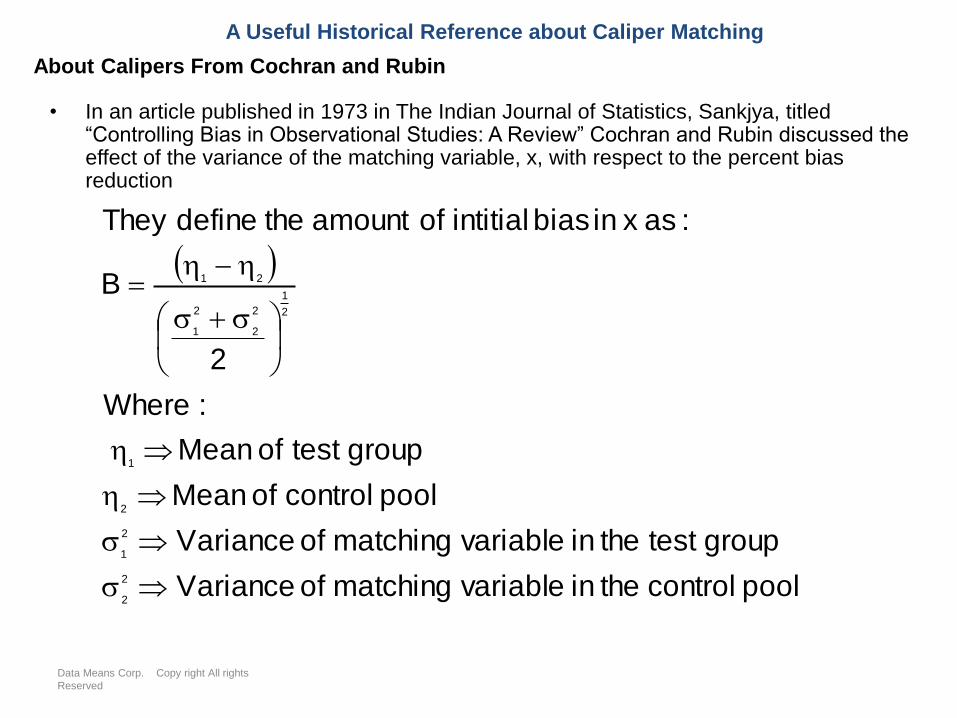
• In an article published in 1973 in The Indian Journal of Statistics, Sankjya, titled “Controlling Bias in Observational Studies: A Review” Cochran and Rubin discussed the effect of the variance of the matching variable, x, with respect to the percent bias reduction

pool control the in variable matching of Variance

group test the in variable matching of Variance

pool control of Mean

group test of Mean

:Where

2

B

:as x in bias intitial of amount the defineThey

2

2

2

1

2

1

2

1

2

2

2

1

21

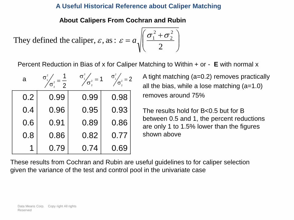
About Calipers From Cochran and Rubin

A Useful Historical Reference about Caliper Matching


Reserved

2

:as , caliper, thedefinedThey 2

2

2

1

a

0.2 0.99 0.99 0.98

0.4 0.96 0.95 0.93

0.6 0.91 0.89 0.86

0.8 0.86 0.82 0.77

1 0.79 0.74 0.69

2

12

2

2

1

The results hold for B<0.5 but for B

between 0.5 and 1, the percent reductions

are only 1 to 1.5% lower than the figures

shown above

a 22

2

2

1

12

2

2

1

Percent Reduction in Bias of x for Caliper Matching to Within + or - E with normal x

A tight matching (a=0.2) removes practically

all the bias, while a lose matching (a=1.0)

removes around 75%

About Calipers From Cochran and Rubin

A Useful Historical Reference about Caliper Matching

These results from Cochran and Rubin are useful guidelines to for caliper selection

given the variance of the test and control pool in the univariate case


Reserved

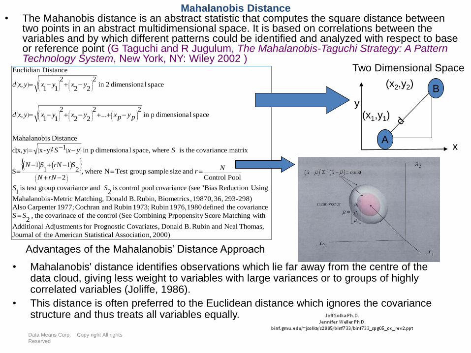
Mahalanobis Distance• The Mahanobis distance is an abstract statistic that computes the square distance between

two points in an abstract multidimensional space. It is based on correlations between the variables and by which different patterns could be identified and analyzed with respect to base or reference point (G Taguchi and R Jugulum, The Mahalanobis-Taguchi Strategy: A Pattern Technology System, New York, NY: Wiley 2002 )

(x1,y1)

(x2,y2)

y

x

B

A

2000) n,Associatio lStatisticaAmerican theof Journal

Thomas, Neal andRubin B. Donald ,Covariates Prognosticfor sAdjustment Additional

with Matching Scorey Prpopensit Combining (See control theof covarinace the, 2

covariance thedefined 1980 1976,Rubin 1973;Rubin andCochran 1977;Carpenter Also

298)-293 36, 19870, ,Biometrics Rubin, B. Donald Matching, Metric-sMahalanobi

UsingReduction Bias" (see covariance pool control is 2

and covariance group test is 1

Pool Control and size sample groupTest N where,

22

11

1S

matrix covariance theis wherespace, ldimensiona pin 1y-xyx,d

Distance sMahalanobi

space ldimensiona pin 2

...2

22

2

11,

space ldimensiona 2in 2

22

2

11,

DistanceEuclidian

SS

SS

Nr

rNN

SrNSN

SyxSt

pypxyxyxyxd

yxyxyxd

Two Dimensional Space

Advantages of the Mahalanobis’ Distance Approach

• Mahalanobis' distance identifies observations which lie far away from the centre of the data cloud, giving less weight to variables with large variances or to groups of highly correlated variables (Joliffe, 1986).

• This distance is often preferred to the Euclidean distance which ignores the covariance structure and thus treats all variables equally.

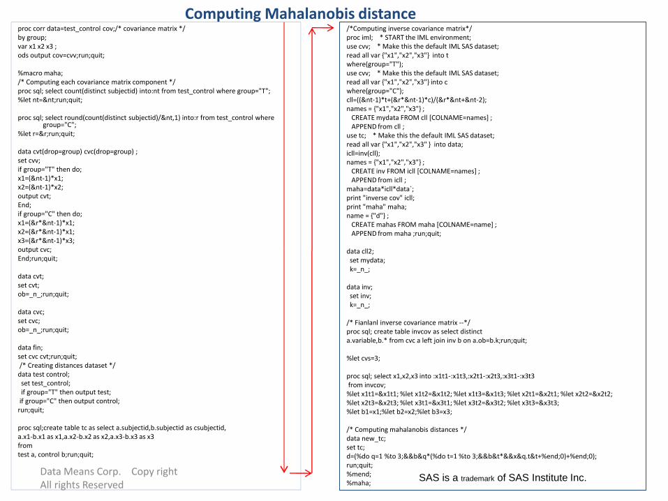
proc corr data=test_control cov;/* covariance matrix */by group;var x1 x2 x3 ;ods output cov=cvv;run;quit;

%macro maha;/* Computing each covariance matrix component */proc sql; select count(distinct subjectid) into:nt from test_control where group="T";%let nt=&nt;run;quit;

proc sql; select round(count(distinct subjectid)/&nt,1) into:r from test_control where group="C";

%let r=&r;run;quit;

data cvt(drop=group) cvc(drop=group) ;set cvv;if group="T" then do;x1=(&nt-1)*x1; x2=(&nt-1)*x2; output cvt;End;if group="C" then do;x1=(&r*&nt-1)*x1; x2=(&r*&nt-1)*x1; x3=(&r*&nt-1)*x3; output cvc;End;run;quit;

data cvt;set cvt;ob=_n_;run;quit;

data cvc;set cvc;ob=_n_;run;quit;

data fin;set cvc cvt;run;quit;/* Creating distances dataset */data test control;set test_control;if group="T" then output test;if group="C" then output control;run;quit;

proc sql;create table tc as select a.subjectid,b.subjectid as csubjectid,a.x1-b.x1 as x1,a.x2-b.x2 as x2,a.x3-b.x3 as x3fromtest a, control b;run;quit;

/*Computing inverse covariance matrix*/proc iml; * START the IML environment;use cvv; * Make this the default IML SAS dataset;read all var {"x1","x2","x3"} into t where(group="T");use cvv; * Make this the default IML SAS dataset;read all var {"x1","x2","x3"} into c where(group="C");cll=((&nt-1)*t+(&r*&nt-1)*c)/(&r*&nt+&nt-2);names = {"x1","x2","x3"} ;

CREATE mydata FROM cll [COLNAME=names] ; APPEND from cll ;

use tc; * Make this the default IML SAS dataset;read all var {"x1","x2","x3" } into data; icll=inv(cll);names = {"x1","x2","x3"} ;

CREATE inv FROM icll [COLNAME=names] ; APPEND from icll ;

maha=data*icll*data`;print "inverse cov" icll;print "maha" maha;name = {"d"} ;

CREATE mahas FROM maha [COLNAME=name] ; APPEND from maha ;run;quit;

data cll2;set mydata;k=_n_;

data inv;set inv;k=_n_;

/* Fianlanl inverse covariance matrix --*/proc sql; create table invcov as select distinct a.variable,b.* from cvc a left join inv b on a.ob=b.k;run;quit;

%let cvs=3;

proc sql; select x1,x2,x3 into :x1t1-:x1t3,:x2t1-:x2t3,:x3t1-:x3t3from invcov; %let x1t1=&x1t1; %let x1t2=&x1t2; %let x1t3=&x1t3; %let x2t1=&x2t1; %let x2t2=&x2t2; %let x2t3=&x2t3; %let x3t1=&x3t1; %let x3t2=&x3t2; %let x3t3=&x3t3;%let b1=x1;%let b2=x2;%let b3=x3;

/* Computing mahalanobis distances */data new_tc;set tc;d=(%do q=1 %to 3;&&b&q*(%do t=1 %to 3;&&b&t*&&x&q.t&t+%end;0)+%end;0);run;quit;%mend;%maha;

Computing Mahalanobis distance

Data Means Corp. Copy rightAll rights Reserved

SAS is a trademark of SAS Institute Inc.

Data Means Corp. Copy right All rights Reserved

matrix covariance theis

distance. smahalanobi with theup come we

metric distnce in the variablesamongn correlatio theeincorporat toreasoningsimilar a Using

ellipsoidan ofequation theisWhich

)(

,....,b ,....,a

ation. transforma requiresch center whi thefrom distance thecomputingen account wh into

x ofty variabili the take tolike would wedistance thisgcalculatinin However,

center thefrom x of distance thefashion to same in the contributex

n observatioan of components allin which spheroid a ofequation theSatisfying

1

,....2,1

1

2

2

1

1

2

2

1

1

1y-xd

Distance sMahalanobi

c1 2

2...

2

2

22

1

10,

,

2

...

2

2

222

1

11,

c 2

...2

2

2

12

xof normEuclidian theis 0, So

..00,0,0,0...y all that assume sLet'

S

sssdiagDWhere

yxDyx

s

y

s

y

s

y

s

x

s

x

s

x

yxS

xDTx

p

s

x

s

x

s

xxd

bad

spypx

s

yx

s

yxbad

xTxpxxxx

xd

T

T

p

t

p

p

p

p

p

In the Euclidian distance

formulation there is an assumption

So all the off Diagonal elements of

D are zero.

The Mahalanobis distance assumes

correlations and that is why we use

the full covariance matrix.

When choosing a distance metric

its is important to understand how

the variables are correlate and

distributed.

The Mahalnobis distance has a

quadratic form

Mahalanobis Distance

form quadratic haswhich

then

and let

1

1

Azzyxsyx

sAyxz

tt


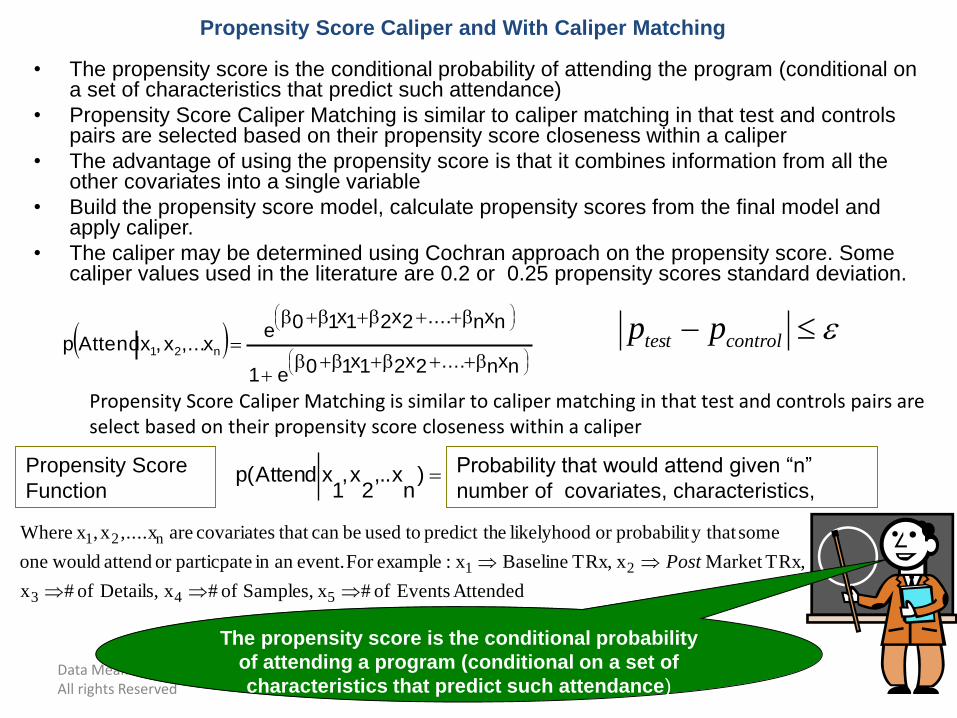
Propensity Score Caliper and With Caliper Matching

• The propensity score is the conditional probability of attending the program (conditional on a set of characteristics that predict such attendance)

• Propensity Score Caliper Matching is similar to caliper matching in that test and controls pairs are selected based on their propensity score closeness within a caliper

• The advantage of using the propensity score is that it combines information from all the other covariates into a single variable

• Build the propensity score model, calculate propensity scores from the final model and apply caliper.

• The caliper may be determined using Cochran approach on the propensity score. Some caliper values used in the literature are 0.2 or 0.25 propensity scores standard deviation.

The propensity score is the conditional probability

of attending a program (conditional on a set of

characteristics that predict such attendance)

controltest pp

nxn....2x21x10e1

nxn....2x21x10ex,...x,xAttendp n21

Propensity Score Caliper Matching is similar to caliper matching in that test and controls pairs are select based on their propensity score closeness within a caliper

)n

x,..2

x,1

xAttend(pPropensity Score

Function

Probability that would attend given “n”

number of covariates, characteristics,

Attended Events of # xSamples, of # xDetails, of #x

TRx,Market xTRx, Baselinex:exampleFor event.an in particpateor attend wouldone

somey that probabilitor likelyhood epredict th toused becan that covariates are ,....xx, xWhere

543

21

n21

Post

Copy Right - All Rights Reserved

11 Data Means

nxn....2x21x10e1

nxn....2x21x10ex,...x,xAttendp n21

nn22110x....xx

p1

pln

One functional form commonly used for the propensity score is the logistic probability

function that has the following exponential form:

After taking the natural log, it acquires a linear form and becomes:

scoeficient regression are ....., , , Wheren210

The Propensity Score

Propensity Score Caliper and With Caliper Matching

x

This is how the

logistic function

looks like!

The advantage of using the propensity score is that it combines information from all the other covariates into a single variable

Why must we estimate the probability that a subject receives a certain treatment since we know for certain which treatment was given? An answer to this question is that if we use the probability that a subject would have been treated (that is the propensity score) to adjust our estimate of the treatment effect, we can create a ‘quasi randomized’ experiment. (“Propensity Score Methods for Bias Reduction in the Comparison of a treatment to a non-randomized control group”, Ralph B D’Agostino. Jr, Statistics in Medicine, 2265-2281, 1998)


Validating your Propensity Scores Approach

Donald B. Rubin recommends the following benchmarks to propensity scores matching 1. The difference in the means of the two groups being compared must be small (e.g. means

must be at least half standard deviations apart).2. The ratio of the variance of the propensity scores of the two groups must be closed to one

(1/2 or 2 may be two extreme).3. The ratio of the variance of the residuals of the covariates after adjusting for the propensity

score must be closed to one. (Regress each of the covariates on the estimated linear propensity score and then take the residual of this regression).

See “Using Propensity Scores to Help Design Observational Studies: Application to the Tobacco Litigation”, Donald B. Rubbin, Health Services & Outcomes Research Methodology, 2, 2001, 169-188

Other general recommendations are:

•For important covariates look at the variance ratio between the test and control pool used Cochran table to get a sense of bias reduction.

•Look closely at the coefficients on your propensity score model. Large coefficients may indicate a poor model.

•Be aware of models with only intercept components (no significant factors). Zero propensity score variance.


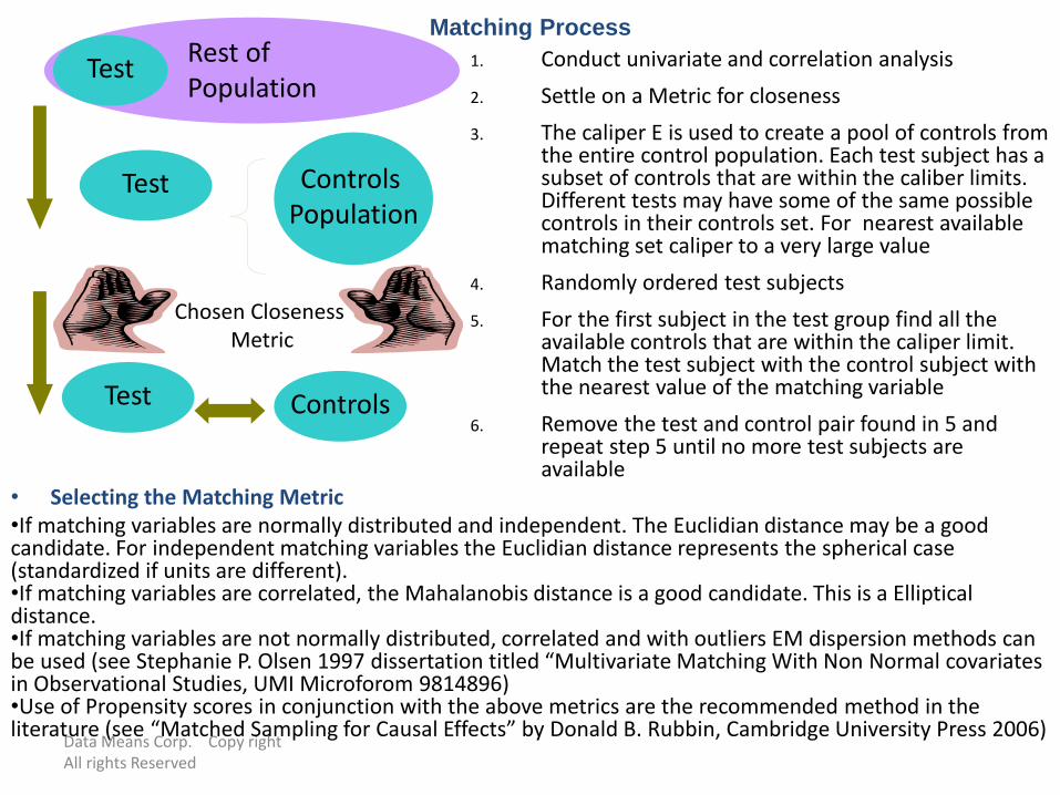
Matching Process

1. Conduct univariate and correlation analysis

2. Settle on a Metric for closeness

3. The caliper E is used to create a pool of controls from the entire control population. Each test subject has a subset of controls that are within the caliber limits. Different tests may have some of the same possible controls in their controls set. For nearest available matching set caliper to a very large value

4. Randomly ordered test subjects

5. For the first subject in the test group find all the available controls that are within the caliper limit. Match the test subject with the control subject with the nearest value of the matching variable

6. Remove the test and control pair found in 5 and repeat step 5 until no more test subjects are available

Test

Test Controls Population

Test Controls

Rest of Population

Chosen ClosenessMetric

• Selecting the Matching Metric•If matching variables are normally distributed and independent. The Euclidian distance may be a good candidate. For independent matching variables the Euclidian distance represents the spherical case (standardized if units are different).•If matching variables are correlated, the Mahalanobis distance is a good candidate. This is a Elliptical distance.•If matching variables are not normally distributed, correlated and with outliers EM dispersion methods can be used (see Stephanie P. Olsen 1997 dissertation titled “Multivariate Matching With Non Normal covariates in Observational Studies, UMI Microforom 9814896)•Use of Propensity scores in conjunction with the above metrics are the recommended method in the literature (see “Matched Sampling for Causal Effects” by Donald B. Rubbin, Cambridge University Press 2006)


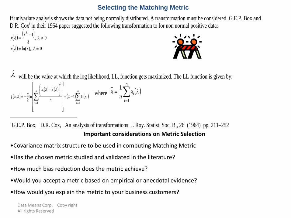
Selecting the Matching Metric

Important considerations on Metric Selection

•Covariance matrix structure to be used in computing Matching Metric

•Has the chosen metric studied and validated in the literature?

•How much bias reduction does the metric achieve?

•Would you accept a metric based on empirical or anecdotal evidence?

•How would you explain the metric to your business customers?

If univariate analysis shows the data not being normally distributed. A transformation must be considered. G.E.P. Box and

D.R. Coxi in their 1964 paper suggested the following transformation to for non normal positive data:

0 ),ln(

0 ,1

xx

xx

will be the value at which the log likelihood, LL, function gets maximized. The LL function is given by:

n

i

i

n

i

i

xn

xxn

xf

11

2

ln1

ln2

,

where

n

i

ixn

x

1

_ 1

i G.E.P. Box, D.R. Cox, An analysis of transformations J. Roy. Statist. Soc. B , 26 (1964) pp. 211–252


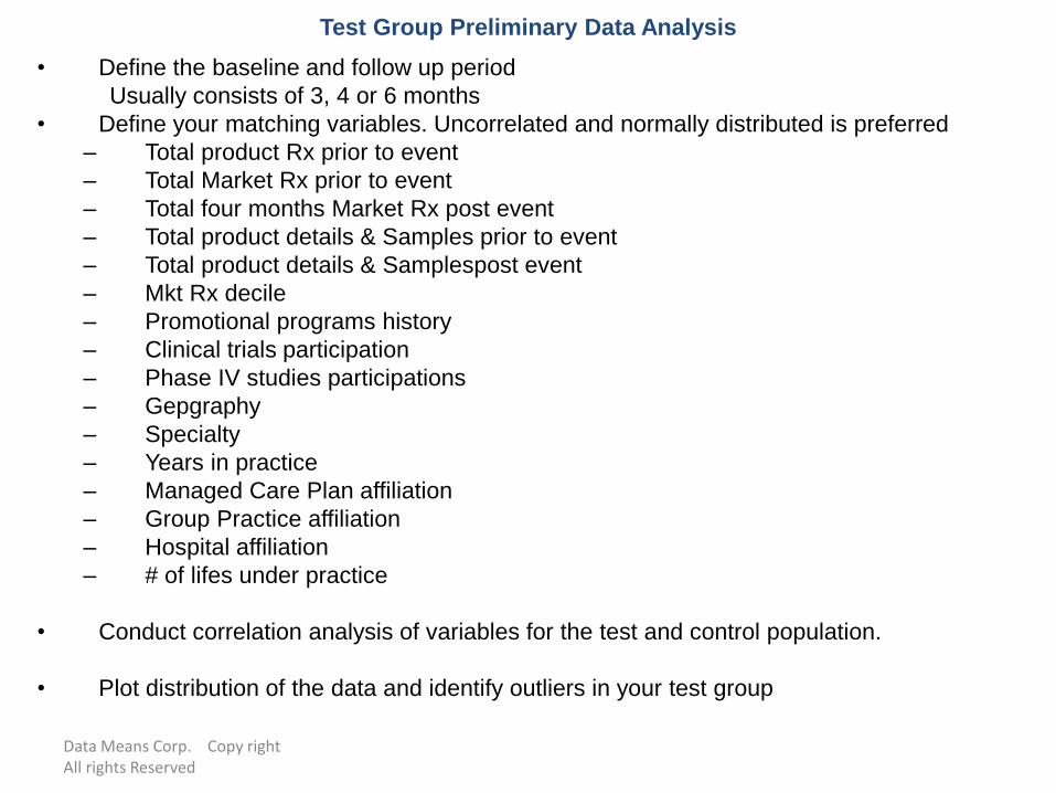
Test Group Preliminary Data Analysis

• Define the baseline and follow up period

Usually consists of 3, 4 or 6 months

• Define your matching variables. Uncorrelated and normally distributed is preferred

– Total product Rx prior to event

– Total Market Rx prior to event

– Total four months Market Rx post event

– Total product details & Samples prior to event

– Total product details & Samplespost event

– Mkt Rx decile

– Promotional programs history

– Clinical trials participation

– Phase IV studies participations

– Gepgraphy

– Specialty

– Years in practice

– Managed Care Plan affiliation

– Group Practice affiliation

– Hospital affiliation

– # of lifes under practice

• Conduct correlation analysis of variables for the test and control population.

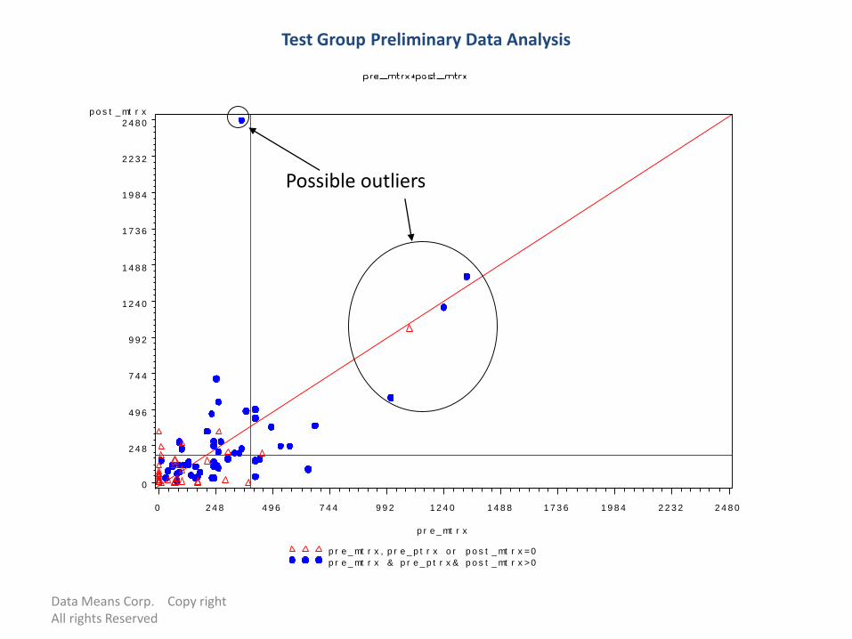
• Plot distribution of the data and identify outliers in your test group


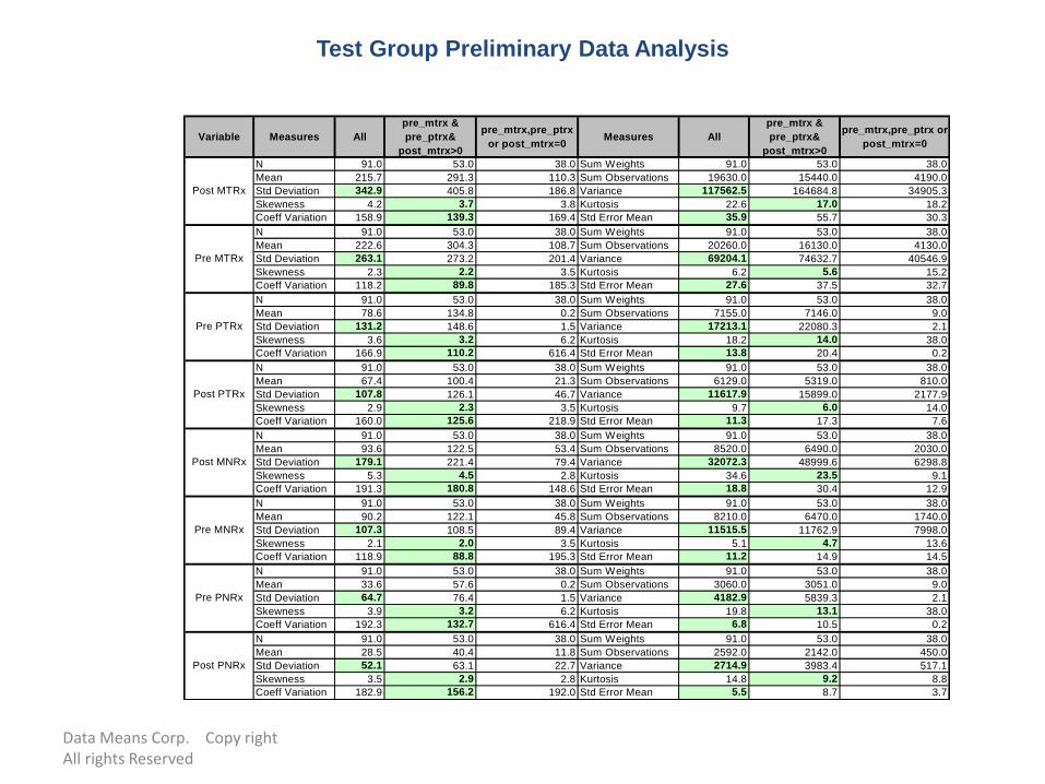
Variable Measures All

pre_mtrx &

pre_ptrx&

post_mtrx>0

pre_mtrx,pre_ptrx

or post_mtrx=0Measures All

pre_mtrx &

pre_ptrx&

post_mtrx>0

pre_mtrx,pre_ptrx or

post_mtrx=0

N 91.0 53.0 38.0 Sum Weights 91.0 53.0 38.0

Mean 215.7 291.3 110.3 Sum Observations 19630.0 15440.0 4190.0

Std Deviation 342.9 405.8 186.8 Variance 117562.5 164684.8 34905.3

Skewness 4.2 3.7 3.8 Kurtosis 22.6 17.0 18.2

Coeff Variation 158.9 139.3 169.4 Std Error Mean 35.9 55.7 30.3

N 91.0 53.0 38.0 Sum Weights 91.0 53.0 38.0





N 91.0 53.0 38.0 Sum Weights 91.0 53.0 38.0





N 91.0 53.0 38.0 Sum Weights 91.0 53.0 38.0





N 91.0 53.0 38.0 Sum Weights 91.0 53.0 38.0





N 91.0 53.0 38.0 Sum Weights 91.0 53.0 38.0





N 91.0 53.0 38.0 Sum Weights 91.0 53.0 38.0





N 91.0 53.0 38.0 Sum Weights 91.0 53.0 38.0





Post PNRx

Post PTRx

Post MNRx

Pre MNRx

Pre PNRx

Post MTRx

Pre MTRx

Pre PTRx



p r e _ mt r x , p r e _ p t r x o r p o s t _ mt r x = 0

p r e _ mt r x & p r e _ p t r x & p o s t _ mt r x > 0

p o s t _ mt r x

0

2 4 8

4 9 6

7 4 4

9 9 2

1 2 4 0

1 4 8 8

1 7 3 6

1 9 8 4

2 2 3 2

2 4 8 0

p r e _ mt r x

0 2 4 8 4 9 6 7 4 4 9 9 2 1 2 4 0 1 4 8 8 1 7 3 6 1 9 8 4 2 2 3 2 2 4 8 0

Possible outliers


Actual #sThis study consisted in analyzing the impact of a pharmaceutical disease management program

which goal was to increase adherence to treatment and increase total prescriptions, TRx.

Pharmaceutical company provided disease management treatment tools to physicians to help

their patients understand treatment and cope with side effects. A retrospective analysis of

physicians prescribing patterns was used to determine the effectiveness of the program.

104 physicians were enrolled for the program however the analysis focused on 91 physicians that

had active prescribing activity before or after the program.

To measure the impact of the program retrospectively a control groups of physicians that did not

participate in the program was chosen using a one to one matching method. Product TRx, Market

Trx were six months prior and market TRx during the program were used as matching variables.

Nearest Neighborhood matching was analyzed using the following matching metrics :

1. Euclidian distance

2. Mahalanobis distance

3. Mahalanobis distance including the propensity score.

4. Propensity Scores

On first look, the Euclidian method produces the best test and control matches. Donald B.

Rubbins, “Matched Sampling for Causal Effects”, Cambridge , June 2006 explains different

methods to build control groups. Propensity scores, and Mahalanobis distance including the

propensity scores are discussed in details and appear to be the prefer methods.

To come up with the propensity scores different models were tried. Trx data was broken down by

volume to come up with the best model.

56 models were tried and analyzed. To select the best model the following criteria were used:

1. R2

2. Model Significance

3. Significance in the model parameters

4. Not statistical differences between test & control groups on selected matching variables

5. Model variables , degrees of freedom

Actual #s

Table below shows the definition of the variables in the best models that were selected.

Variables were recoded using the test group data as reference to ensure adequate cell

frequencies. All the other models failed in significance levels of the model parameters or overall

model. Not effort was made to fit any model that would produce the best matching control but

that will violate fundamental statistical assumptions. Recoded Variables Description

btrxc Pre Product Trx Category

amtrxc Post Mkt Trx Category

qpre_mnrx Distributional Quartile(0-25, 25-50, '50-75, 75+) based on Test Group Pre Mkt Nrx

qpost_mnrx Distributional Quartile(0-25, 25-50, '50-75, 75+) based on Test Group Post Mkt Nrx

qpre_mtrx Distributional Quartile(0-25, 25-50, '50-75, 75+) based on Test Group Pre Mkt Trx

qpost_mtrx Distributional Quartile(0-25, 25-50, '50-75, 75+) based on Test Group Post Mkt Trx

shr Pre Trx Share

qpre_pnrx Distributional Quartile(0-25, 25-50, '50-75, 75+) based on Test Group Pre Product Nrx

Pre Product Trx category and “amtrxc” is Post Mkt Trx category. These variables were defined

as: Recode Post Mkt Trx

0 0 1240

1 1240 2480Post Mkt Trx

Recode Pre Product Trx

0 0 670

1 670 1340Pre Product Trx

The best four models.

Model R

Max-Rescale

R Square

Intercept

Only

Model

Model With

Intercept &

Covariates

Intercept

Only

Model

Model With

Intercept &

Covariates

Intercept

Only

Model

Model With

Intercept &

Covariates

btrxc amtrxc 0.272% 3.6% 1099.1 1060.8 1101.134 1066.8 1108.7 1089.5

qpre_mnrx qpost_mnrx 0.158% 2.1% 1099.1 1076.9 1101.134 1082.9 1108.7 1105.5

qpre_mtrx qpost_mtrx 0.173% 2.3% 1099.1 1074.8 1101.134 1080.8 1108.7 1103.5

shr qpre_pnrx 0.105% 1.4% 1099.1 1084.3 1101.134 1090.3 1108.7 1113.0

- 2 Log L AIC SC


Actual #s

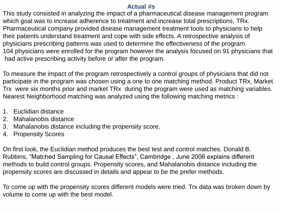
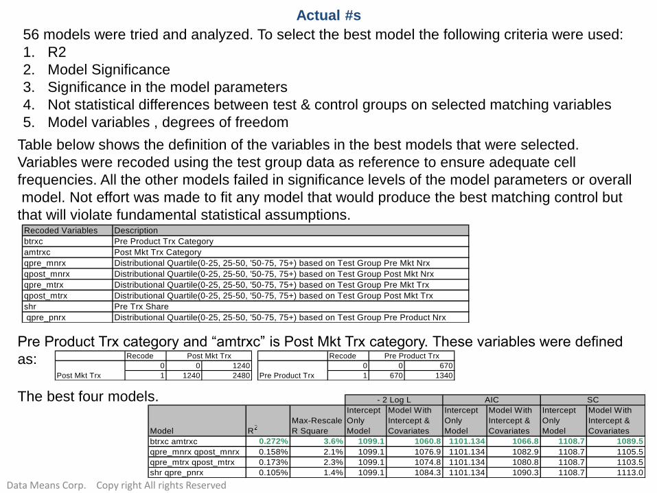
The first model was selected because it had the highest R2, and lowest -2 Log L, AIC and SC values.

The second and third models may show some correlation between the variables. In that market

volume is constant. The last model may have some challenges since Share is a continuous variable

and was not categories. Values with share missing due to market volume equals to zero may

influence model results. The following table shows the results of the test and control differences

using these four models:

Model Difference Low CL Mean Upper CL Standar Error

Post Mkt Trx -131.9 -46.6 38.7 43.2

Pre Mkt Trx -134.9 -68.2 -1.6 33.8

Pre Product Trx -56.4 -23.9 8.5 16.4

Post Mkt Trx -107.1 -17.3 72.6 45.6

Pre Mkt Trx -90.2 -14.6 61.0 38.3

Pre Product Trx -42.9 -0.1 42.7 21.7

Post Mkt Trx -118.7 -34.7 49.2 42.5

Pre Mkt Trx -97.5 -26.8 43.9 35.8

Pre Product Trx -52.2 -18.8 14.6 16.9

Post Mkt Trx -149.8 -66.8 16.1 42.0

Pre Mkt Trx -109.7 -37.7 34.4 36.5

Pre Product Trx -42.9 -5.1 32.6 19.1

btrxc amtrxc

qpre_mnrx qpost_mnrx

qpre_mtrx qpost_mtrx

shr qpre_pnrx

The third model, (propensity

score(qpre_mnrx qpost_mnrx) without

caliper), produced the best results that

will not violate the ANCOVA

assumptions with regards to pre

product Trx, Pre and post market Trx.

Results showed that there was

not significant effect on the

group variable for the first six

months after the program

however, a significant effect

was observed after the first 12

months. Indicating a possible

lag effect while the program got

on its way and gained traction.


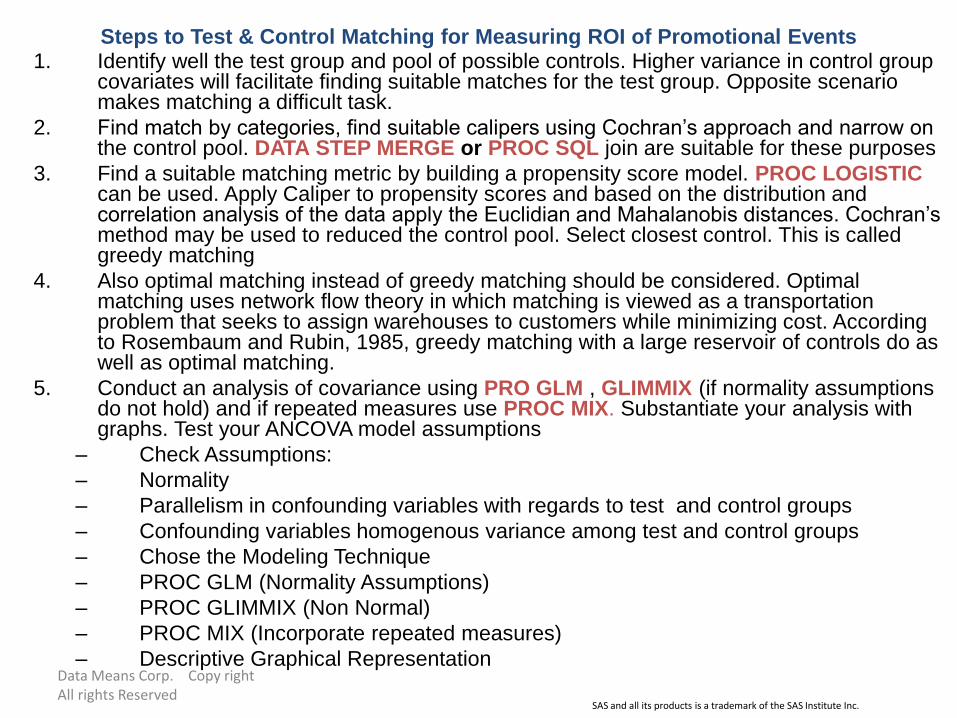
1. Identify well the test group and pool of possible controls. Higher variance in control group covariates will facilitate finding suitable matches for the test group. Opposite scenario makes matching a difficult task.

2. Find match by categories, find suitable calipers using Cochran’s approach and narrow on the control pool. DATA STEP MERGE or PROC SQL join are suitable for these purposes

3. Find a suitable matching metric by building a propensity score model. PROC LOGISTICcan be used. Apply Caliper to propensity scores and based on the distribution and correlation analysis of the data apply the Euclidian and Mahalanobis distances. Cochran’s method may be used to reduced the control pool. Select closest control. This is called greedy matching

4. Also optimal matching instead of greedy matching should be considered. Optimal matching uses network flow theory in which matching is viewed as a transportation problem that seeks to assign warehouses to customers while minimizing cost. According to Rosembaum and Rubin, 1985, greedy matching with a large reservoir of controls do as well as optimal matching.

5. Conduct an analysis of covariance using PRO GLM , GLIMMIX (if normality assumptions do not hold) and if repeated measures use PROC MIX. Substantiate your analysis with graphs. Test your ANCOVA model assumptions

– Check Assumptions:

– Normality

– Parallelism in confounding variables with regards to test and control groups

– Confounding variables homogenous variance among test and control groups

– Chose the Modeling Technique

– PROC GLM (Normality Assumptions)

– PROC GLIMMIX (Non Normal)

– PROC MIX (Incorporate repeated measures)

– Descriptive Graphical Representation

Steps to Test & Control Matching for Measuring ROI of Promotional Events

SAS and all its products is a trademark of the SAS Institute Inc.


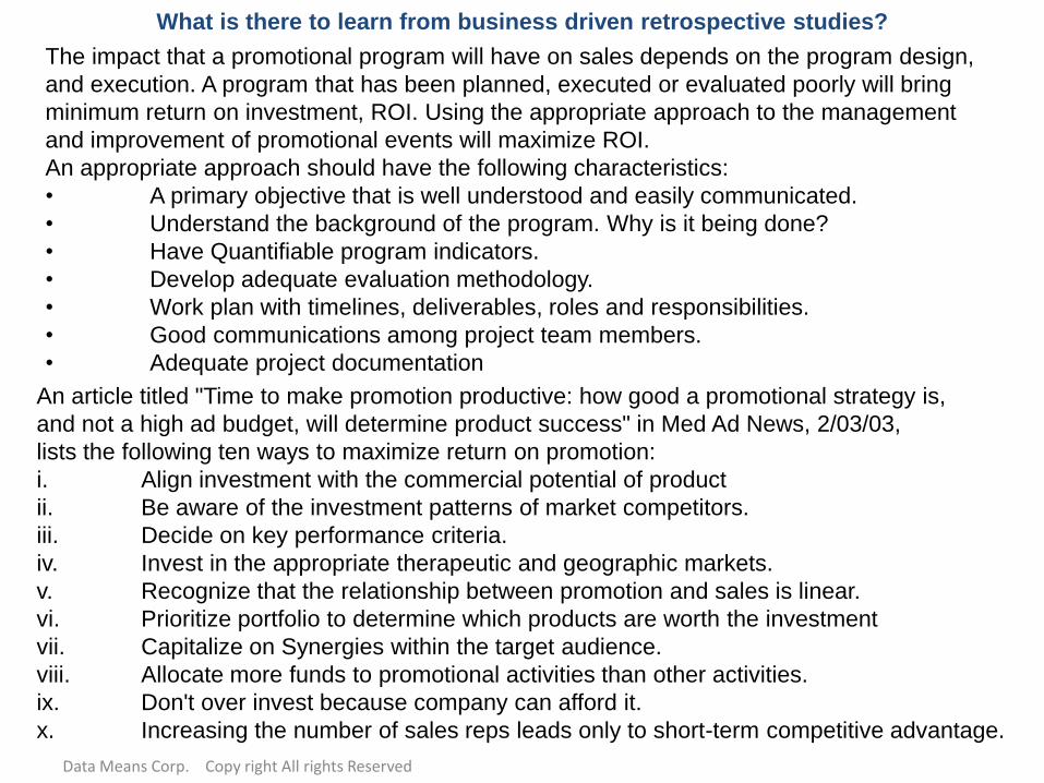
What is there to learn from business driven retrospective studies?

The impact that a promotional program will have on sales depends on the program design,

and execution. A program that has been planned, executed or evaluated poorly will bring

minimum return on investment, ROI. Using the appropriate approach to the management

and improvement of promotional events will maximize ROI.

An appropriate approach should have the following characteristics:

• A primary objective that is well understood and easily communicated.

• Understand the background of the program. Why is it being done?

• Have Quantifiable program indicators.

• Develop adequate evaluation methodology.

• Work plan with timelines, deliverables, roles and responsibilities.

• Good communications among project team members.

• Adequate project documentation

An article titled "Time to make promotion productive: how good a promotional strategy is,

and not a high ad budget, will determine product success" in Med Ad News, 2/03/03,

lists the following ten ways to maximize return on promotion:

i. Align investment with the commercial potential of product

ii. Be aware of the investment patterns of market competitors.

iii. Decide on key performance criteria.

iv. Invest in the appropriate therapeutic and geographic markets.

v. Recognize that the relationship between promotion and sales is linear.

vi. Prioritize portfolio to determine which products are worth the investment

vii. Capitalize on Synergies within the target audience.

viii. Allocate more funds to promotional activities than other activities.

ix. Don't over invest because company can afford it.

x. Increasing the number of sales reps leads only to short-term competitive advantage.



Common problems in promotional programs are:

1. Method for selecting physicians invited to the program is poor. Detail profile of attendees is

unknown. Project manager knows conceptually who is to be invited to the program but lack

controls to ensure who gets invited in reality. Project manager does not know exactly who was

invited and attended the program. There is not master list of invitees with appropriate ME

numbers or database identifiers.

2. There are not reporting requirements for agencies. Agency submits contact information of

program attendees to project manager.

3. Attendees contact information needs to be matched against databases to get ME number.

4. There is not evaluation of the program by the attendees.

5. For those attendees that are not physicians, there is not follow up to understand their

relationship with the physicians the program is trying to impact.

6. Data is not produced in a timely fashion.

7. There is not standard ROI methodology making it hard to compare programs.

8. There is not database that tracks physician participation, programs characteristics and

outcomes.

A promotional program must be well structured to ensure its success. The idea that a promotional

program must be developed and analyze without any rigor must be abandoned. In the same way

that Clinical studies must be well designed to proof or support the benefits of a treatment,

promotional programs must be developed and conducted with the due diligence to be able to

measure their effectiveness.


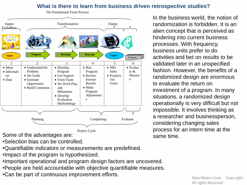
The Promotional Event Process

Inputs Transformation Output

Evaluation

1 2 3 4 5 6

Ideas

Informati

on

Data

Understand the

Problem

Set Goals

Estimate

Opportunity

Build Consensus

Develop

Program

Get Support

Form Team

Set Work Plan

and

Milestones

Develop

Evaluation

Methodology

Run

Program

Review

Interim

Results

Make

Program

Adjustment

s

NRx

Sales

Producti

vity

Gains

Evalua

te &

Measur

e

Planning Completing Evaluate

Project Cycle

Inputs Prepare Develop Execute

Output

Evaluate

In the business world, the notion of

randomization is forbidden. It is an

alien concept that is perceived as

hindering into current business

processes. With frequency,

business units prefer to do

activities and bet on results to be

validated later in an unspecified

fashion. However, the benefits of a

randomized design are enormous

to evaluate the return on

investment of a program. In many

situations, a randomized design

operationally is very difficult but not

impossible. It involves thinking as

a researcher and businessperson,

considering changing sales

process for an intern time at the

same time. Some of the advantages are:

•Selection bias can be controlled.

•Quantifiable indicators or measurements are predefined.

•Impact of the program is hypothesized.

•Important operational and program design factors are uncovered.

•People are held accountable with objective quantifiable measures.

•Can be part of continuous improvement efforts.




Recommendation for Program Evaluations

1. Build an evaluation design early on the project development phase to make sure that required data is capture adequately. Randomized design is the preferred method.

2. Settle on matching and outcomes variables.

3. When doing matching conduct preliminary data analysis to understand correlation, distributions and detect outliers in the matching variables. Transformed variables to make them normal.

4. Select matching metric that is in accordance with findings in #3.

5. If propensity scores are used Don’t let the data or software determined your model. Build an appropriate model that is simple, statistically sound and does not violate statistical assumptions.

6. Compare variance in test group and control population with regards to matching variables. If test to control population variance ratio is greater than 1 you may want to reconsider your test and control reservoir because the variance of your test is greater than your control pool and percentage reduction bias may be small. Also this may be a sign that there is not overlap in distributions.

7. Do not drop observations for matching. If there are outliers you may want to analyzed them separately after matching

8. If using analysis of covariance, ANCOVA, via a linear model validate assumptions such as:

– Normality

– Parallelism in confounding variables with regards to test and control groups

– Confounding variables homogenous variance among test and control groups

9. Report findings and make recommendations.

10. Be honest and do not massage the data to meet clients business expectations


References

• “The Bias Due to Incomplete Matching”, Paul Rosenbaum, Donald B Rubin, Biometrics 41, March 1985• “Combining Propensity Score Matching With Additional Adjustment for Prognostic Covariates”, Donald B.

Rubin and Neal Thomas, Journal of the American Statistical Association, June 2000• “Controlling Bias in Observational Studies: A Review”, Cochran and Donald Rubin, The Indian Journal of

Statistics, Sankjya, 1973• The Mahalanobis-Taguchi Strategy: A Pattern Technology System, G Taguchi and R Jugulum, New York, NY:

Wiley 2002• “Using Propensity Scores to Help Design Observational Studies: Application to the Tobacco Litigation”,

Donald B. Rubbin, Health Services & Outcomes Research Methodology, 2, 2001, 169-188• Stephanie P. Olsen 1997 dissertation titled “Multivariate Matching With Non Normal covariates in

Observational Studies, UMI Microforom 9814896• “Matched Sampling for Causal Effects” by Donald B. Rubbin, Cambridge University Press 2006• “Outlier Detection and Data Cleaning in Multivariate Non Normal Samples: The PAELLA Algorithm, Manuel

Castejon Limas, Joaquin B Ordieres Mer, Francisco J. Martinez De Pison Escacibar, Eliseo P. Vergara Gonzales, Datamining Knowledge discovery, 9, 171-187, 2004

• “Detection of Outliers in Multivariate Data: A Method Based on clusters and Robust Etimators”, Carla M. Santos-Pereira and Ana M. Pires

Contact Info:

Alejandro Jaramillo, Data Means Corp., www.DataMeans.com

Tel: 732-371-9512

email:[email protected]

Date post:	23-Jan-2018
Category:	Data & Analytics
Upload:	alejandro-jaramillo
View:	88 times
Download:	4 times

2007 Pharmasug, Promotion Response Analysis

Data & Analytics