Interconnection Optimalization of Power Units with Renewable Power Sources (RES) to Distribution Network Tomáš Skočil University of West Bohemia in Pilsen, Faculty of Electrical Engineering Department of Electric Power Engineering and Ecology Univerzitní 26, 306 14 Plzeň, Czech Republic University of Vigo, Higher Technical School of Industrial Engineering Department of Electric Engineering Lagoas – Marcosende, 36202 Vigo, Spain Universidade de Vigo Escola Técnica Superior de Enxefíeiros Industriais de Vigo Departmento de Enxefíeria Eléctrica supervisor: Manuel Pérez Donsión E-mail: [email protected], [email protected]Abstract: This doctoral thesis deals with renewable power sources (RES) which can be connected to the distribution power network in the Czech Republic and in Spain. We mean photovoltaic cells, wind plants, small water power plants, biomass power plants and so on. I try to draw up a specification of problems of renewable energy sources and their power control, because these sources have certain specific features that are given by their characters. I give an attention to the characteristics of the sources that influence the reliability and quality of the power supply. I also deal with this behavior of sources in the distribution grid, their possible influence on a voltage regulation, influence of their power variation on voltage waveform at the point of connection and also an examination of different variants of grid topology for which these sources work considering their operation utility. Keywords: Microgrids, renewable energy, renewable power sources, optimalization, wind power, PV cells, fly-wheels, water power plant, mathematical model of sources, load waveform, Swing
Transcript
Interconnection Optimalization of Power Units with Renewable Power Sources (RES) to Distribution Network
Tomáš Skočil
University of West Bohemia in Pilsen, Faculty of Electrical Engineering
Department of Electric Power Engineering and Ecology Univerzitní 26, 306 14 Plzeň, Czech Republic
University of Vigo, Higher Technical School of Industrial Engineering
Department of Electric Engineering Lagoas – Marcosende, 36202 Vigo, Spain
Universidade de Vigo Escola Técnica Superior de Enxefíeiros
2.1 THE RELATIONSHIP BETWEEN THE MICROGRID AND A LOCAL ELECTRICITY UTILITY .......................................7 2.1.1 Internal control of a microgrid..................................................................................................................8 2.1.2 Power balance...........................................................................................................................................8 2.1.3 Frequency..................................................................................................................................................9 2.1.4 Voltage ....................................................................................................................................................10 2.1.5 Power quality ..........................................................................................................................................10 2.1.6 Energy balance........................................................................................................................................11 2.1.7 Energy storage ........................................................................................................................................11
3 PARTS OF MICROGRIDS................................................................................................................................13
3.1 PV CELL........................................................................................................................................................13 3.1.1 How solar cells work...............................................................................................................................14
3.3 FULL CELL ....................................................................................................................................................23 3.4 BATTERIES OR FUEL CELLS – WHAT IS BETTER TO USE..................................................................................26
3.4.1 Common Attributes..................................................................................................................................26 3.4.2 Different Attributes..................................................................................................................................27 3.4.3 Capacity Variation ..................................................................................................................................29 3.4.4 Flexibility in Operation ...........................................................................................................................30 3.4.5 Comparing of batteries and fuel cells......................................................................................................33
4 REAL PV SYSTEM ON THE ROOF OF FACULTY OF ELECTRICAL ENGINEERING......................37
4.1 PARAMETERS OF PV ARRAY .........................................................................................................................37 4.2 MEASUREMENT OF REAL VALUES OF DAILY IRRADIATION............................................................................39
5 MATHEMATICAL MODELLING AND SIMULATION OF PV ARRAY.. ................................................42
5.1 MATHEMATICAL MODEL OF PV CELL ...........................................................................................................42 5.1.1 Parameters of PV cell for normal specification ......................................................................................45 5.1.2 Equation describing a behavior of PV cell..............................................................................................46
5.2 APPLICATION OF PV CELL MODEL IN COMPUTER PROGRAM SWING ..............................................................48 5.2.1 Controlix..................................................................................................................................................48 5.2.2 Application in Swing ...............................................................................................................................48 5.2.3 Results from Controlix for various parameters .......................................................................................53
6 COMPARISON OF PARAMETERS – MODEL AND REAL SYSTEM ... ...................................................57
9 LIST OF FIGURES.............................................................................................................................................65
As conventional fossil-fuel energy sources diminish and the world’s environmental concern about
acid deposition and global warming increases, renewable energy sources (solar, wind, tidal, and
geothermal, etc.) are attracting more attention as alternative energy sources. Among the renewable
energy sources solar photovoltaic (PV) energy has been widely utilized in small-size applications.
It is also the most promising candidate for research and development for large-scale uses as the
fabrication of less-costly photovoltaic devices becomes a reality. PV power generation, which
directly converts solar radiation into electricity, contains a lot of significant advantages such as
inexhaustible and pollution-free, silent and with no rotating parts, and size-independent electricity
conversion efficiency. Positive environmental effect of photovoltaic is replacing electricity
generated in more polluting way or providing electricity where none was available before. With
increasing penetration of solar photovoltaic devices, various anti-pollution apparatuses can be
operated by solar PV power; for example, water purification by electrochemical processing or
stopping desert expansion by photovoltaic water pumping with tree implantation. From an
operational point of view, a photovoltaic array experiences large variations of its output power
under intermittent weather conditions. Those phenomena may cause operational problems at a
central control centre in a power utility, such as excessive frequency deviations, spinning reserve
increase, etc.
One method to overcome the above problem is to integrate the PV power plant with other power
sources such as diesel backup, fuel cell backup, battery backup, and superconductive magnetic
energy storage (SMES) backup. The diesel backup for PV power is able to make a continuous 24-
hour power supply be possible. However, it has a couple of severe drawbacks. Its electricity
efficiency decreases significantly at a low level of power output, and the diesel power generation is
environmentally detrimental as well. The SMES technology is many years from
commercialization, and there is a significant potential health risk associated with the technology
because of its strong magnetic field generation.
Almost all the electricity currently produced in the Czech Republic (Spain) is generated as part of
a centralised power system designed around large fossil fuel or nuclear power stations. This power
system is robust and reliable but the efficiency of power generation is low, resulting in large
quantities of waste heat. The principal aim of this project is to investigate an alternative concept:
Microgrid
3
the energy production by small scale generators in close proximity to the energy users, integrated
into microgrids.
2 MICROGRID
General definition - a microgrid is an integrated energy system consisting of interconnected loads
and distributed energy resources which as an integrated system can operate in parallel with the grid
or in an intentional island mode1.
Microgrids is the decentralised electricity generation combined with production of heat - bear the
promise of substantial environmental benefits, brought about by a higher energy efficiency and by
facilitating the integration of renewable sources such as photovoltaic arrays or wind turbines. By
virtue of good match between generation and load, microgrids have a low impact on the electricity
network, despite a potentially significant level of generation by intermittent energy sources.
Figure 1: Stand-alone microgrid at night
Figure 2: Stand-alone microgrid in the day-time
Microgrid
4
A microgrid is a small-scale power supply network that is designed to provide power for a small
community, for example a typical housing estate, isolated rural communities, to mixed suburban
environments, academic or public communities such as universities or schools, to commercial
areas, industrial sites and trading estates, or municipal regions.
Figure 3: Electric power network - microgrid Advantages and disadvantages of microgrid
The use of renewable energy sources for the generation of electricity is seen as one of the
important ways of reducing carbon dioxide emissions. Whilst some of these sources can produce
large power outputs in single power stations – for example hydropower or geothermal power. The
majority are relatively small in size. This means such generators are more conveniently (and
cheaply) connected at lower voltages within the distribution system. It was never envisaged that
this system would be required to support the connection of generation. A similar situation exists
with combined heat and power (CHP) units which produce both electricity and heat.
Approximately, almost 50% of the primary energy consumption is used to provide heating and hot
water in buildings and the aim of CHP is to supply this low-grade heat alongside electricity
generation. The advantages of a high overall efficiency of energy production which are thus
attained must be offset against the necessity to operate smaller units close to the consumer, and the
usually the need to operate a district heating system to distribute the heat.
Microgrid
5
The term “distributed generation” is used to describe these generators (typically small renewables
and CHP but also other on-site electricity generators) connected to the distribution system. A
synonymous term also used is “embedded generation”, describing generators embedded within the
distribution system. Connection of generation in this way poses many technical, commercial and
safety issues; all of which must be tackled in order to allow a wide penetration of renewable
generation. In addition to the problems posed by distributed generation, the use of renewable
sources and CHP usually adds more specific issues related to the actual method of generation used.
An example that can be used to illustrate this point is photovoltaic (PV) generation. There is no
generation at night, which is of course predictable but in addition, the sun can be obscured by
cloud cover on a random basis. A similar situation exists with CHP which is normally controlled to
supply heat, with electricity production as a by-product. These phenomena change in all time
scales leading to a constantly changing electrical output. As a source of electrical energy this has
some disadvantages which, in the present format, have to be addressed by the operators of the
public electricity supply. Consumers have become used to electrical power available on demand.
They do not need to structure their load pattern, the entire responsibility for matching power and
demand is placed upon the utilities which must have enough generation available at all times. With
more creative thinking about the way energy is supplied, used and controlled it may be possible to
satisfy the demand for energy but accommodate the fluctuating resources which are a feature
particularly of renewable energy sources. This may be possible by ensuring a satisfactory mixture
of sources and loads to enable the demand and supply to match.
Problems of microgrids
Although examples of networks similar to microgrids exist, there are technical and regulatory
issues that need to be considered before this concept can apply on a wider scale. The principal
issue to consider is how closely the energy supply (both electricity and heat) within the microgrid
can satisfy the local loads. The answer to this question will help decide how the microgrid interacts
with the main utility, and the nature of the connection to be determined. Indeed, it may even be
desirable in some circumstances for the microgrid to be disconnected from the utility, and operate
as “stand-alone”. The issues that must be resolved to permit this type of operation include:
1. Precise energy and power balance within the microgrid, on a time scale ranging from
milliseconds to years. Over the short time scale, the power balance is linked to the question of
control; over longer time scales, one needs to consider the relationship between energy supply,
Microgrid
6
demand and storage. Similar arguments are used to design stand-alone power supplies, for
example, photovoltaic or hybrid systems which power remote equipment or serve isolated rural
communities across the world.
2. The nature of connection with the main utility (the “grid connection”). An arrangement which
would permit the microgrid operator the choice to operate in the “grid connected” or “stand alone”
mode is an uncharted territory for conventional power utility engineers, and issues remain both at
the technical and regulatory level.
3. Energy storage. The conventional utility supply operates on the principle that power is generated
when it is required. Energy storage introduces a novel component in a utility supply and broadens
the design criteria. On a quantitative level, the size of the energy store is intimately linked to the
energy balance and to the required security of supply provided by the microgrid.
4. Demand management. The temporal mismatch between generation and load can be alleviated by
managing the demand. The shifting of load facilitates achieving the energy balance and helps
reduce the size of energy storage. Whilst experience exists of demand-side management at
industrial level and lessons can be learned from concepts such as storage heating, demand
management at the domestic level is attracting much interest in the research community but further
experience is needed before routine applications become commonplace.
5. Seasonal match between generation and load Energy storage and demand management can be
effective to achieve energy balance at the diurnal time scale. A sufficient energy must be available
from the generators to ensure energy balance over longer time scales if a microgrid powered by
renewable or other intermittent energy sources such as micro-CHP is to be capable of stand alone
operation. This can usually be achieved only by a diversity of generation methods appropriate to
the load.
Why to use microgrids?
The motivation behind use of microgrids lies in the potential of the microgrid concept to deliver a
significant reduction of CO2 emissions, for the following reasons:
• The use of both electricity and heat permitted by the close proximity of the generator to the
user, thereby increasing the overall energy efficiency
Microgrid
7
• Significant environmental benefits made possible by the use of low or zero emission
generators including PV arrays and fuel cells etc.
• Low impact on the electricity network, by virtue of good match between generation and
load, despite a potentially significant level of generation by intermittent energy sources
The feature of the microgrid is that it should be local electricity generation that matches the power
requirements in the microgrid. There are various types of generator that may be considered.
Photovoltaic cells are attractive if the environment is primarily residential since they may be
incorporated into buildings in an unobtrusive manner. Very small scale cogeneration schemes can
be based on gas boilers for central heating and domestic hot water. Possible technologies for this
are fuel cells or Stirling Engine powered generators. For a microgrid including commercial or light
industrial premises then larger cogeneration schemes based on gas turbines or other prime movers
may become appropriate.
Energy storage will probably be required to accommodate the variations of available generation
and power demand. Short term storage of electrical power will be necessary to help accommodate
the rapid fluctuations of load or generation that may be anticipated on a small power network.
Over longer time scales, energy management made possible by storage can be used to make the
most efficient use of photovoltaic generation or the electricity produced by micro-CHP. Some
energy storage may be possible in the form of domestic hot water or as part of space heating.
2.1 The relationship between the microgrid and a local electricity utility
The intention is that the microgrid can be self sufficient, but for security of supply and flexibility it
would almost certainly be connected to the local electrical utility network, or even to adjacent
microgrids. These links may be bi-directional enabling the import or export of electricity, or,
depending on commercial considerations, it might just be a unidirectional flow of power. From the
point of view of the microgrid the utility connection might be viewed just as another generator or
load.
This raises the question as to whether or not the microgrid should be linked to other networks over
a synchronous alternating current (AC) connection. The advantage of a synchronous link would be
its simplicity, requiring only an electrical interconnection, circuit breakers and probably a
transformer. Lasseter has considered this possibility and shown that in principle it should be
possible to run a microgrid with minimal central control of local generation which is able to
operate connected to the utility, or, in the event of loss of the connection, move smoothly into
Microgrid
8
stand-alone or island operation with no loss of power to the microgrid. What is perhaps less clear
is how the synchronous connection would be re-synchronised once the utility was ready to re-
establish the connection.
The alternative approach would be an asynchronous connection using a direct current (DC)
coupled electronic power converter. This might be bi-directional, enabling import and export of
power or simply device to import power when local resources were inadequate. An advantage of
this approach is that it isolates the microgrid from the utility as regards reactive power, load
balance etc. Only power is exchanged with the utility, the microgrid is entirely responsible for
maintaining the power quality (frequency, voltage and supplying reactive power and harmonics)
within its area.
With an asynchronous link the microgrid might be unusual in that all its power will be supplied
through electronic inverters. Some generators, such as photovoltaic cells are intrinsically sources
of DC and hence need inversion to connect them to an AC network. Others, for example
microturbines or Stirling engines may generate AC but are not well suited to operating a
synchronous generator because the frequency is unsuitable or variable. Voltage source inverters
with suitable control schemes will be required to permit stable operation of the network with many
small generators attached. Fortunately advances in power electronics and digital controllers mean
that sophisticated control strategies are possible and the cost need not be excessive. Which of these
approaches is more appropriate may well depend on the size of the microgrid. It may also depend
on the regulatory environment governing the interchange of power between the microgrid and the
utility.
2.1.1 Internal control of a microgrid
There are many commercial and political issues concerned with control; however the technical
problems of a microgrid must be managed, for the concept to become a reality. The control of a
microgrid is intimately tied with the energy and power balance in the microgrid, and the question
of energy storage. There are three main parameters – frequency, voltage and power quality - that
must be considered and controlled to acceptable standards whilst the power and energy balance is
maintained.
2.1.2 Power balance
A power system usually contains no significant energy storage; the generated and dissipated power
must therefore be constantly kept in balance. This power balance must be maintained on a cycle by
Microgrid
9
cycle basis if the system is to maintain its frequency. Too much generation and the system
accelerates, too little and it slows; neither situation is acceptable.
In a microgrid, frequency stability becomes critical; therefore control is a major concern. There are
a number of techniques used to restore the power balance and hence correct the frequency: the use
of load shedding, increase in primary generation and recovery of stored energy. All of these are
available within a microgrid, but because the system is small the problem is much more difficult to
manage to the same standard as is normal in a utility system.
Short term storage of energy is needed to cope with the fluctuations in power demand or
accommodate the sudden loss of some generation. A microgrid with many small generators will
not be an intrinsically stiff system, unlike a national interconnected utility. The small generators
will neither store significant energy in their mechanical inertia, nor will they necessarily respond
quickly to sudden changes of load. Short term storage, probably distributed, with the generators
will permit the inverters to follow the rapidly changing demand while giving time for the
generators to respond, or extra generation to be brought on line or for generators to be closed
down. This same storage could be used to help accommodate the diurnal variation of demand.
There are two related issues, firstly quite small power imbalances will produce large frequency
excursions and secondly they will happen much more quickly. The first issue may also be an
advantage for a microgrid since small energy stores will have significant effects. The second issue
means that stored energy recovery must be fast and precise. Since the most probable store, in the
near future is likely to be a battery with an inverter, this does not pose an insurmountable problem;
such a system is quite fast enough to ensure adequate frequency control.
2.1.3 Frequency
Power system operates at 50Hz and there are obvious advantages in adopting this frequency,
whether there is to be a synchronous connection or not. The frequency limits are laid down by law
and are relatively tight though not to the same standards as some other power systems. There is
however no reason to adopt these standards and some relaxation could be possible (in a non-
synchronous system) if it were advantageous. It is doubtful however, that limits larger than ±0.5
Hz could be acceptable. Frequency therefore must be controlled to within these limits.
The “normal” method of frequency control power system is by control of the rotational speed of
the synchronous machines supplying the power. Within a large interconnected system, with many
Microgrid
10
synchronous generators, no single machine can control the frequency, there being a flow of
“synchronic power” into any machine that is slowed in order to keep it in synchronism. There
needs to be a large power imbalance to alter the speed and hence frequency of the system.
The fewer the number of machines, the less stiff the system and frequency control becomes a
technical issue. Machines in such a system must be able to respond quickly to load variations in
order to preserve the power balance at all times. This means rapid detection of frequency change
and fast, accurate control of load generation, or both.
Not all renewable generators are synchronous machines: wind turbines are often induction
generators and photovoltaic arrays connect to the system through inverters. These two require very
different frequency and load control in order to satisfactorily operate in a system. Inverters can be
used to control frequency since the inverter frequency can be controlled independently of load.
However, inverters do not behave as rotational synchronous generators and require different
philosophies.
2.1.4 Voltage
The system voltage within a large multi generator system is controlled by initially the voltage of
the machines but also by the reactive flow. In general, the reactive balance becomes more critical
in a smaller system. For example, all reactive demand must be supplied from one generator in a
single machine system. This is not strictly true, but adds significantly to cost and control problems
if reactive demand has to be compensated by extra static plant.
A conventional distribution system is usually a feeder network, and there is little interconnection.
Voltage drop along feeders becomes an issue, as it will vary with load and distance along the
feeder. This dictates that any simple microgrid will have to be either small to be satisfactory or be
specially designed as an interconnected network.
The voltage and its limits at consumer’s terminals are specified by law, but they are reasonably
wide. With proper design, production of the correct voltage should not be an insurmountable
problem.
2.1.5 Power quality
Control of power quality will be the biggest issue for a microgrid. Voltage dips, flickers,
interruptions, harmonics, dc levels, etc. will all be more critical in a small system with few
Microgrid
11
generators. There will need to be a critical appraisal of both the effects and consequences of
relaxing and/or enforcing standards in this area.
The distributed generation within the microgrid could enable better control of power quality. With
electrical storage together with the distributed generation power quality could be maintained in
much the same way as is achieved by Uninterrupted Power Supply (UPS) systems. The electronic
inverters can not only supply power at the fundamental frequency, they can also generate reactive
power to supply the needs of reactive loads, cope with unbalanced loads and generate the harmonic
currents needed to supply non-linear loads.
2.1.6 Energy balance
Little significance is usually attached to the concept of energy balance in a conventional system:
the solution is just to add more fuel over time. A microgrid which contains a high proportion of
intermittent energy sources - be it renewables such as PV or wind or energy sources controlled for
other purposes such as micro- CHP - is not able to do this. The energy available to the system is
finite and depends on matters that cannot usually be controlled or even predicted with any
certainty.
If such a source is to be used and achieve levels of reliability similar to those of conventional plant,
energy storage is essential. It is also clear that, as the diversity of the generation methods in any
system is reduced, the role of energy storage becomes more dominant. It therefore appears
desirable that any microgrid should employ more than one method of generation as well as some
form of energy store.
The diversity of generation methods is particularly important if the microgrid is to operate stand
alone. The microgrid must then contain sufficient generation capacity and type that can supply
adequate amounts of energy with sufficient reliability. Photovoltaic arrays, for example, are a
reliable power source during the summer months. They combine well with generators such as
micro-CHP which generate most power in winter to provide heat for domestic dwellings.
2.1.7 Energy storage
There is no economic general purpose method for the storage of electricity per se in the quantities
required for public utility use. There are of course methods involving capacitors and super
conducting magnets; both of which are technically complex and with present knowledge, rather
expensive, but nevertheless used in specific situations. Because the direct storage of electricity is
Microgrid
12
not very practical, the storage of energy by other methods, for later use in electricity generation is
employed. These are many and varied, depending upon the situation and the purpose for which the
electricity is to be used.
It is likely that a microgrid will rely on chemical energy storage in the form of electric batteries. In
the simplest of systems this will mean lead acid cells, which are well developed, available,
predictable and robust. For more sophisticated applications, redox batteries are becoming
available, and development will continue. In critical situations, where cost is not an issue, the
application of super conducting energy storage has been used. Again, continued development is
expected to both reduce costs and to increase reliability. Over shorter periods of time, the use
flywheels may be appropriate.
The calculation of battery size (energy), and inverter rating (power), will depend on the size of the
loads and generators within the microgrid, as well as its topography. As an alternative to storing
energy, the shedding of load is more likely to be used in a microgrid, rather than a large scale
public utility, because it is easier to identify those loads which are least critical. Where
cogeneration is used, some of this energy storage may well be in the form of heat. This storage
could be in the form of domestic hot water or stored for use in space heating. Innovative control
strategies can be developed to make use of this storage and, if necessary, the plant may be run to
meet the electrical load when there is no demand for thermal energy.
Parts of microgrids
13
3 PARTS OF MICROGRIDS
3.1 PV cell
As PV cell manufacturing technologies improve steadily, commercial applications of PV power
generation have increased from stand-alone to utility-connected generating systems.
Interconnection and operation of a PV power unit are not same as electric utilities have been doing
for the conventional power plants. It requires specific PV interface, protection schemes, storage
devices, and control mechanisms. Especially because the PV power output is directly affected by
the changes of weather (solar intensity, temperature, etc.), it becomes considerably complicated to
efficiently control the PV power plant.
Solar cells represent the fundamental power conversion unit of a photovoltaic system. They are
made from semiconductors, and have much in common with other solid-state electronic devices,
such as diodes, transistors and integrated circuits. For practical operation, solar cells are usually
assembled into modules.
Many different solar cells are now available on the market, and yet more are under development.
The range of solar cells spans different material and different structures in the quest to extract
maximum power from the device while keeping the cost to a minimum. Devices with efficiency
exceeding 30% have been demonstrated in the laboratory. The efficiency of commercial devices,
however, is usually less than half this value.
Crystalline silicon cells hold the largest part of the market. To reduce the cost, these cells are now
often made from multicrystalline material, rather than from the more expensive single crystals.
Crystalline silicon cell technology is well established. The modules have along lifetime (20 years
or more) and their best production efficiency is approaching 18%.
Cheaper (but also less efficient) types of silicon cells, made in the form of amorphous thin films,
are used to power a variety of consumer products. You will be familiar with the solar-powered
watches and calculators, but larger amorphous silicon solar modules are also available.
A variety of compound semiconductors can also be used to manufacture thin-film cells (for
example, cadmium telluride or copper indium diselenide). These modules are now beginning to
appear on the market and hold the promise of combining low cost with acceptable conversion
efficiencies.
Parts of microgrids
14
A particular class of high-efficiency solar cells from single crystal silicon or compound
semiconductors (for example, gallium arsenide or indium phosphide) is used in specialised
applications, such as to power satellites or in system which operate under high-intensity
concentrated sunlight.
Photovoltaic materials are not restricted to semiconductors. Solar cells are now available which
convert light to electricity by organic modules, with best conversion efficiency exceeding 10%.
3.1.1 How solar cells work
The solar cell operation is based on the ability of semiconductors to convert sunlight directly into
electricity by exploiting the photovoltaic effect. In the conversion process, the incident energy of
light creates mobile charged particles in the semiconductor which are then separated by the device
structure and produce electrical current.
Figure 4: shows the diagram of silicon cell, the typical solar cell in use today. The electrical
current generated in the semiconductor in extracted by constants to the front and rear of the cell.
The top contact structure which must allow light to pass through is made in the form of widely-
spaced thin metal strips (usually called “fingers”) that supply current to a large bus bar. The cell is
covered with a thin layer of dielectric material – the antireflection coating or ACR – to minimize
light reflection from the top surface.
Figure 4: The silicon solar cell
Figure 5 a) shows the band diagram of the semiconductor section under illumination. Light
generates electron-hole pairs on the both sides of the junction, in the n-type emitter and in the p-
type base. The generated minority carriers – electrons from the base and holes from the emitter –
then diffuse to the junction and are swept away by the electric field, thus producing electric current
Parts of microgrids
15
across the device. Note how the electric current of the electrons and holes reinforce each other
since these particles carry opposite charges. The p-n junction therefore separates the carries with
opposite charge, and transforms the generation current Il between the bands into an electric current
across the p-n junction. The I-V characteristic of a solar cell can be obtained by drawing an
equivalent circuit of the device (Figure 6). The generation of current Il by light is represented by a
current generator in parallel with a diode which represents the p-n junction. The output current I is
then equal to the difference between the light-generated current Il and the diode current ID.
Equation
−
= 1exp0 kT
qVII
then gives
−
−= 1exp0 kT
qVIII l
Note that, under open circuit when I=0, all the light-generated current passes through the diode.
Under short circuit (V=0) on the other hand, all this current passes through the external load. The
I-V characteristic and its relationship to the diode characteristic are shown in Figure 6.
Figure 5: schematic representation of different types of photovoltaic converters. a) Currents in a p-n junction under illumination (applicable, for example, to crystalline silicon or gallium arsenide solar cells), b) the band diagram and operation of p-i-n amorphous silicon solar cells, c) energy conversion by a dye-
sensitised photochemical solar cell
Parts of microgrids
16
The I-V characteristic contains several important points. One is the short-circuit current ISC which,
as we noted, is simply the light-generated current Il. The second is the open-circuit voltage VOC
obtained by setting I=0:
+= 1ln
O
lOC I
I
q
kTV
Figure 6: equivalent circuit and I-V characteristic of a solar cell compared to a diode
It is worthwhile to examine this equation in more detail. Both Il and IO depend on the structure of
the device. However, it is the value of IO – which can vary by many orders of magnitude,
depending on the device geometry and processing-that determinates the open circuit voltage in
practical devices.
No power is generated under short or open circuit. The maximum power Pmax produced by the
device is reached at a point on the characteristic where the product IV is maximum. This is shown
graphically in Figure 24 where the position of the maximum power point (A) represents the largest
area of the rectangle shown. One usually defines the fill factor by
SCOCmm IVFFIVP max ==
where Vm and Im are the voltage and current at the maximum power point.
The efficiency η of a solar cell is defined as the power Pmax produced by the cell at the maximum
power point under standard test conditions, divided by the power of the radiation incident upon it.
Parts of microgrids
17
Most frequent conditions are: irradiance 100mW/cm2, standard reference AM1.5 spectrum, and
temperature 25°C. The use of this standard irradiance value is particularly convenient since the cell
efficiency in percent is then numerically equal to the power output from the cell in mW/cm2. Other
test conditions are sometimes adopted for cells which operate in a different environment, for
example, cells which power satellites and operate under AM0 spectrum.
The I-V characteristic which we have derived for a simplified device describes, in fact, rather well
the operation of solar cells in practise if the parameters make allowance for the losses which take
place in practical devices.
Gallium arsenide solar cells (Figure 7) are, because of their high cost, usually intended for
operation on satellites or in concentration system. Gallium arsenide is a direct-gap semiconductor
and most photons of light are absorbed in the top emitter layer. The top “windows” layer prevents
these carries diffusing to the top surface and being lost by surface recombination.
Figure 7: The structure and band diagram of gallium arsenide soalr cells
Most thin-film solar cells are made from amorphous or polycrystalline semiconductors with low
diffusion constant for electrons and holes. To aid the carrier transport, these cells usually
incorporate a lightly doped or intrinsic layer as part of the junction where most of the light is
absorbed. Electrons and holes which are created in this layer are then pulled apart by the electric
field immediately after their creation, eliminating carrier diffusion to the junction.
Semiconductors need not form the key element of solar cell operation. Working solar cells have
now been manufactured where the charge separation step is mediated by a molecular dye. In these
devices, the dye layer covers a nanocrystalline titanium oxide electrode which acts as a receptor
for electrons from the photoexcited dye molecules. The nanocrystalline structure of the titanium
oxide particles assists efficient light absorption even by a very thin dye layer, which is probably
monomolecular. The positive electrode is formed by a hole-carrying redox electrolyte.
Parts of microgrids
18
3.2 Battery
Another important element of microgrids is the battery. It is necessary in such a system because of
the fluctuating nature of the output delivered by the PV arrays. Thus, during the hours of sunshine,
the PV system is directly feeding the load, the excess electrical energy being stored in the battery.
During the night or during the period of low solar irradiation energy is supplied to the load from
the battery.
3.2.1 Introduction (Lead-Acid Battery)
A storage battery is a chemical device reversible in its action, which stores chemical energy for use
later as electrical energy. The chemical energy stored in electrodes of a battery cell is converted to
electrical energy when the cell is discharging. Electrical energy is applied to the battery during the
operation of charging, so the electric current produces chemical changes in the battery.
The most commonly used storage battery for utility applications is the lead-acid type. The
fundamental parts of a lead-acid battery cell are two dissimilar electrodes immersed in an
electrolyte, namely
Anode(-) : Spongy lead (Pb) Cathode(+) : Lead dioxide (PbO2) Electrolyte : Dilute solution of sulfuric acid (H2SO4)
When a battery cell is connected to a circuit, it allows charge to flow around the circuit. In its
external part, the charge flow is electrons resulting in electrical current. Within the cell, the charge
flows in the form of ions that are transported from one electrode to the other. The cathode, highly
oxidized lead dioxide, receives electrons from the external circuit on discharge. These electrons
react with the cathode material, which leaves some lead free to combine with sulphate ions to form
lead sulphate. Hydrogen ions move in to the cathode and combine with oxygen to form water. At
the anode, reactions between the anode material and the sulphate ions result in excessive electrons
that can be donated to the external circuit. In this way the chemical energy stored in the battery is
converted to electrical energy.
The chemical reaction occurred at the anode is
−− + ←
→+ ePbSOSOPb
ech
edisch
24arg
arg24
and that at the cathode is
Parts of microgrids
19
OHPbSOeHSOPbOech
edisch
24arg
arg242 224 +
← →
+++ −+−
Therefore, the net reaction can be expressed as follows
OHPbSOSOHPbPbOech
edisch
24arg
arg
422 222 + ←
→++
A battery system is a group of battery cells that supply DC power at a nominal voltage to an
electrical load. The number of cells connected in series determines the nominal voltage of the
battery system, and the capacity of the battery system is the basic factor in determining the
discharge rate. The voltage is the force enforcing each of the electrons coming out of the battery
and the capacity is the number of electrons that can be obtained from the battery. While the voltage
is fixed by cell chemistry, the capacity is variable depending on the quantity of active materials.
The discharge rate of a battery is given in terms of ampere-hours (Ah) to a particular discharge
voltage level. For the lead-acid battery, its nominal cell voltage is 2V and the nominal discharge
voltage level is 1.75 V/cell, or approximately 87.5 % of the nominal cell voltage rating. The
equivalent circuit for a battery is shown in Figure 8.
Figure 8: Equivalent circuit for a battery Rov - overvoltage resistance Cov - overvoltage capacitance Rbat - internal resistance Rb - self-discharge resistance Cb - battery capacitance Voc - open circuit voltage V - battery voltage
The internal resistance is due to the resistance of electrolyte and electrode. Self-discharge
resistance is a result of electrolysis of water at high voltages and slow leakage across the battery
terminals at low voltages. The over-voltage is simulated as an RC circuit with a time constant in
the order of minutes. Lead-acid battery systems are a near-term solution to power regulation needs
for electric utilities. However, the technology has suffered from a slow acceptance into power
Parts of microgrids
20
markets due to such factors as uncertain return on investment and difficulty in quantifying benefits.
Recently, there is worldwide interest to develop alternatives to lead-acid batteries that are able to
produce high performance at low cost. Advanced batteries such as nickel-cadmium, sodium-sulfur
and zinc-bromine are likely to emerge in the next decade.
3.2.2 Nickel-Cadmium Battery
As the nickel-cadmium battery promoters claim its superiority over the lead-acid batteries in spite
of the high capital cost, there are several tries to adopt the nickel-cadmium batteries for use in PV
applications. One major reason for that is its longer life and operational reliability. It is undamaged
by complete discharge and overcharge.
The active material of the cathode is nickel hydrate with graphite and that of the anode is cadmium
sponge, with additives to aid conductivity. The electrolyte is a solution of potassium hydroxide
(KOH), including a small amount of lithium hydroxide (LiOH) to improve capacity. The charge-
discharge reaction may be written as
22arg
arg
3 )()(2)(2 OHCdOHNiCdOHNiech
edisch
+ ←
→+
The nominal voltage of a nickel-cadmium battery on discharge is 1.2 V. When the battery is
connected to an external load, its voltage falls to a value depending on discharge rate and state of
charge. The normal final discharge voltage is 1.05 V/cell. The battery is characterized by a low
self-discharge rate; its capacity drops to about 80 % in a year under open circuit conditions. Its
operating temperature range is between -50 to 60 °C and the battery capacity drops to half of the
nominal capacity at -50 °C.
Nickel-cadmium battery system contains its significant features for PV applications. With respect
to charging conditions, the nickel-cadmium battery offers more than 80% charging efficiency, as
high as a lead-acid battery does. It does not suffer from complete discharge or overcharge in
contrast to the lead-acid battery and its annual maintenance is less costly that that of the lead-acid
battery. At low temperatures there is a need for the lead-acid battery to be kept in a high state of
charge to avoid freezing, which would make it less cost effective over the nickel-cadmium battery.
A disadvantage associated with the nickel-cadmium battery is its memory effect and high capital
cost. Repeated use in the same way causes the battery to adjust itself to a certain capacity in
relation to its load. Its cost per ampere-hour of capacity is considered as another disadvantage for
Parts of microgrids
21
wide use although the battery is promoted as an alternative to the lead-acid battery in PV
applications.
3.2.3 Sodium-Sulfur Battery
The sodium-sulfur battery operates at relatively high temperature ranging from 300°C to 380°C in
order to maintain the sodium, sulfur and reaction products in liquid forms and to obtain adequate
electrolyte conductivity. Unlike conventional battery systems that consist of solid electrodes and
liquid electrolytes for the reaction medium, the sodium-sulfur battery is based on liquid electrodes
and a β-alumina (Al2O3) solid electrolyte. The battery uses molten sodium and molten sulfur as
active materials for the anode and the cathode, respectively. Its operation relies on the property of
β-alumina, which combines very low electronic conductivity with an unusually high ionic
conductivity, especially to sodium ions. The overall chemical reaction can be written as
32arg
arg
32 SNaSNaech
edisch
← →
+
The operating discharge voltage characteristics are somewhat lower than those of lead-acid
batteries. The sodium-sulfur battery would start at around 1.9 V and finish at about 1.4V.
The sodium-sulfur battery possesses several potential advantages for energy storage applications.
It is capable of quick responses to sudden changes from charge to discharge conditions and vice
versa, as well as sudden changes in load demand. Its capital cost is projected to be low compared
to other advanced battery systems because the battery component materials are relatively abundant
and inexpensive. A projected installation cost of $100/kWh is believed achievable. Energy
efficiency of the sodium-sulfur battery is high at approximately 80% and it does not self-discharge.
It possesses high volumetric energy density. The projected energy density of the battery is about
200Wh/kg compared to 35Wh/kg for lead-acid batteries.
There are a number of technical issues including cell reliability that must be addressed before the
technology is ready for commercial introduction. Because sodium and sulfur are hazardous
materials, safety and environmental concerns must be considered in its fabrication, operation and
disposal.
Parts of microgrids
22
3.2.4 Zinc-Bromine Battery
The zinc-bromine battery is another promising system for PV power applications due to inherent
chemical simplicity, good electrochemical reversibility of the electrodes and low-cost material. It
is a near-ambient temperature, flowing electrolyte system. Its active materials are stored externally
in anolyte and catholyte reservoirs. Upon charging the battery, an electrolyte solution of zinc
bromine (ZnBr2) is passed through the battery with the aid of a circulator. As dc electricity is
passed through the battery, zinc metal is deposited on the anode, and bromine gas is generated at
the cathode and then is carried away with the circulating electrolyte stream. Upon discharge,
circulation of the aqueous zinc bromine electrolyte carries bromine to the cathode of the stack and
current may be withdrawn from the battery. Microporous polyethylene separators are used to slow
the direct reaction of the bromine-rich stream with zinc. The overall cell reaction is written as
(aq) (g) (s) 2arg
arg
2 ZnBrBrZnech
edisch
← →
+
where s, g, and aq denote solid-, gas-, and aqueous-states, respectively. There are several attributes
of the zinc-bromine battery for applications of future energy storage. The majority of the battery’s
components are made of low-cost, plastic materials. Inexpensive construction materials coupled
with low fabrication expenses result in favorable capital cost projections. It can be assembled in
modular fashion using standard cell stacks, allowing the user to increase capacity to meet future
requirements. The near-ambient temperature operation does not require the complex thermal
management necessary in some high-temperature systems. It can be repeatedly deep discharged
without performance deterioration. Its energy efficiency is not as high as that of the competitors,
roughly 60-70 %.
However, there are a number of key technical issues related to the reliability and performance of
the battery. The efficiency of the battery system is somewhat lower than other systems, due to
resistive losses in the separators, electrolyte, and electrodes. The system’s mechanical complexity
creates a good deal of maintenance requirements including pump repair and stack replacement.
Additionally, the safe handling, storage and disposal of zinc-bromine batteries must be considered
because bromine is a toxic material.
3.2.5 Battery Applications to Power Systems
The future electric power system is estimated to be uncertain and potential capacity shortages,
competitive power markets and increasing environmental regulations will create further stresses on
Parts of microgrids
23
the interconnected power network. The roles of storage facilities, especially a battery energy
storage (BES) system as power regulation and energy management are being recognized as a
practical solution to future operating uncertainty.
BES systems have been interesting power utilities as an option to supply power at peak time to
achieve load levelling. Recently, other dynamic benefits of BES have been identified, such as load
following, spinning reserve, power factor correction, long line stabilization, and voltage and
frequency regulation, etc. The BES system is predicted to become an economically attractive
option for utilities in the future due to those benefits coupled with the ability to provide peak
power.
3.3 Full cell
It looks exceptional that fuel cells have not been widely commercialized for power utility
applications since sulfuric acid fuel cells were invented 150 years ago by an Englishman, William
Grove. The great promise of fuel cells as a means for efficient production of electricity from the
oxidation of a fuel has been recognized again due to the growing interest in environmental concern
about global warming and decreasing conventional power generating sources.
The fuel cell is an electrochemical device that converts the free-energy change of an
electrochemical reaction into electrical energy. The simplest overall fuel cell reaction is
yelectricitOHOH +→+ 222 2
1
The free-energy change of this reaction under standard conditions of temperature and pressure
(25 °C, 1 atm) is 56,32 kCal/mole. The number of electrons transferred in this reaction is 2 and the
reversible potential is 1.229 V. Even if there were no efficiency losses in H2-O2 fuel cells, heat
would still be rejected from a fuel cell. Thus, the theoretical efficiency of the fuel cells at 25 °C is
83 %.
The performance of a fuel cell that operates at low and intermediate temperatures of 25 - 200 °C is
illustrated in Figure 9. That figure, a typical cell voltage versus current density plot, explains the
important role of electrode kinetics on its performance. The following relation may represent the
performance equations when the current density varies from zero to the end of the linear region.
Parts of microgrids
24
Figure 9: Typical plot of cell voltage vs. current density for a fuel cell
ffff RIIbEE −−= log0
Where
00 log frf IbEE +=
The low electrocatalytic activity of most electrode materials for the oxygen electrode reaction
causes the difficulties in attaining high energy efficiencies and high power densities in low- to
medium-temperature fuel cells. Fuel cell performance can be increased by increasing cell
temperature and reactant pressure.
The equivalent circuit for a fuel cell is depicted in Figure 10. The equivalent steady state DC
resistance is high but the transient impedance is low. The low transient impedance will make fuel
cell response much faster than any conventional generating system. It should be remembered that
fuel cells will use the same primary fuels as conventional power generation forms, and fuel cells
must be economically competitive with these conventional systems. Therefore, fuel cells do not
offer a real energy alternative but contribute to energy savings because of their intrinsic high
efficiency. The reliability of fuel cells for steady power generation has been proven in the U.S.
aerospace program. Design reliability (mean time to failure) greater than 95 % has been achieved
consistently under the stringent conditions of space flight. The design reliability required for most
terrestrial uses is lower than those needed for aerospace applications. However, terrestrial units
require reliability during much longer total operating periods. It is expected that the first generation
of commercial fuel cell power generation systems will have an on-stream availability of 90 %.
Ultimately, fuel cell power plants can have on-stream availability of 98 - 99 %.
Parts of microgrids
25
Figure 10: Equivalent circuit of a fuel cell E0 - open circuit voltage R1 - charge transfer resistance C1 - cell capacitance RT - electrolyte resistance LT - equivalent inductance
The high reliability of a fuel cell system will largely result not only from the modularity of the
stacks and stack components, but from their lack of highly stressed moving parts operating under
extreme conditions. It operates under relatively benign conditions, so it can be designed such that
maintenance is required only at infrequent intervals. A plant could be operated at full power during
periods of routine maintenance by replacing spare modules. Without spare parts, plants could be
designed so that only partial shutdown will be necessary in the event of failure. Any low-
temperature fuel cell system must take several fuel-processing steps to produce hydrogen that will
be consumed inside the fuel cell stacks. The most effective way to produce the hydrogen is by
steam-reforming of hydrocarbon fuels. First, fuel purification to avoid poisoning of the steam-
reforming catalyst is required, which is done by hydrodesulfurization. This is followed by
reforming and carbon monoxide (CO) shift reaction to reduce any residual CO values to acceptable
levels. The above reactions are endothermic, so they need a net heat input from the fuel used or
from any available heat. High-temperature heat is required for the reforming, typically 750 –
800 °C. Unless this heat can be given directly by the waste heat from a high-temperature fuel cell,
it must be provided by burning excess fuel.
Fuel cells are known to possess a great number of attributes that make them attractive for the
purpose of power generation. The inherent modularity in their production contains the feature less
sensitive to size. It enables them to be added successively. Fuel cells have high efficiency and
relatively flat efficiency characteristics that make them useful for part-load operation. Fuel cells
can utilize a variety of fuels such as natural gas, coal-derived gas, biogas and methanol, and they
are able to respond very fast to load changes. Their low noise and emissions and negligible water
Parts of microgrids
26
requirements allow them much more flexibility in siting. Because of those benefits, fuel cells have
continuously been under research and development despite their high initial cost right now.
3.4 Batteries or fuel cells – what is better to use
Both batteries and fuel cells have their own unique contributions to electric power systems as
discussed above. Those two power sources also contain a great potential to back up severe PV
power fluctuations under inclement weather conditions. In this chapter comparison between
batteries and fuel cells is carried out in detail only for their PV power backup options, so their
common attributes and different attributes will be discussed.
3.4.1 Common Attributes
Photovoltaic power outputs vary depending mainly upon solar insolation and cell temperature.
Since control of the ambient weather conditions is beyond human beings’ capability, it is almost
impossible for human operators to control the PV power itself. Thus, a PV power generator may
sometimes experience sharp output power fluctuations owing to intermittent weather conditions,
which causes control problems such as load frequency control, generator voltage control and even
system stability analysis. There is, therefore, a need for backup power facilities in the PV power
generation. Batteries and fuel cells are the most likely technologies to provide the PV system with
backup power because these two backup power sources contain some distinct features in common.
Those characteristics are listed below.
• Fast load-response capability: Fuel cells and batteries are able to respond very fast to load
changes because their electricity is generated by chemical reactions. A 14.4kW lead-acid
battery running at 600A has maximum load gradient of 300 A/sec. A phosphoric-acid fuel
cell system can match a demand that varies by more than half its rated output within 0.1
second. The dynamic response time of a 20kW solid-oxide fuel cell power plant is less than
4 second when a load increases from 1 to 100%, and it is less than 2 msec when a load
decreases from 100 to 1%.
• Modularity in production: Factory assembly of standard cell units provides fuel cell and
battery power plants with short lead-time from planning to installation. This modular
production enables them to be added in discrete increments of capacity, which allows better
matching of the power plant capacity to expected load growth. In contrast, the installation
Parts of microgrids
27
of a single large conventional power plant may produce excess capacity for several years,
especially if the load growth rate is low.
• Highly reliable sources: Due to their multiple parallel modular units and absence of
electromechanical rotating masses, fuel cell and battery power plants are more reliable than
any other forms of power generation. Fuel cells are expected to attain performance
reliability near 85%. Consequently, a utility that installs a number of fuel cell or battery
power plants is able to reduce its reserve margin capacity while maintaining a constant
level of the system reliability.
• Flexibility in site selection (Environmental acceptability): The electrochemical conversion
processes of fuel cells and batteries are very quiet because they do not have any major
rotating masses. External water requirement for their operation is, if any, very little while
conventional power plants require massive amount of water for system cooling. Therefore,
they can reduce or eliminate water quality problems created by the conventional plants’
thermal discharges. Air pollutant emission levels of fuel cells and batteries are none or very
little. Emissions of SO2 and NOx in the fuel cell power plant are 0.003 lb/MWh and 0.0004
lb/MWh respectively. Those values are projected to be about 1,000 times smaller than
those of fossil-fuel power plants since fuel cells do not rely on a fuel-burning process.
These environmentally benign characteristics make it possible for those power plants to be
located close to load centers in urban and suburban area. It can also reduce energy losses
and costs associated with transmission and distribution equipment. These siting near load
centers may also reduce the likelihood of system blackouts.
3.4.2 Different Attributes
Electric current is produced in a storage battery by chemical reactions. The same chemical
reactions take place in a fuel cell, but there is a difference between them with respect to fuel
storage. In storage batteries chemical energy is stored in the positive/negative electrodes of the
batteries. In fuel cells, however, the fuels are stored outside the cells and need to be fed into the
electrodes continuously when the fuel cells are required to generate electricity. Other detailed
comparison between battery backup and fuel cell backup for PV power supplement is made in the
following sections.
Efficiency
Parts of microgrids
28
Power generation in fuel cells is not limited by the Carnot Cycle in the view that they directly
convert available chemical free energy to electrical energy rather than going through heat
exchange processes. Thus, it can be said that fuel cells are a more efficient power conversion
technology than the conventional steam-applying power generations. Figure 11 illustrates energy
conversion processes for a conventional power generator and a fuel cell. Whereas the fuel cell is a
one-step process to generate electricity, the conventional power generator has several steps for
electricity generation and each step requires a certain amount of energy loss.
Fuel cell power systems have around 40-60 % efficiencies depending on the type of electrolytes.
For example, the efficiencies of phosphoric-acid fuel cells and molten-carbonate fuel cells are 40-
45 % and 50-60 %, respectively. Furthermore, the fuel cell efficiency is usually independent of
size; small power plants operate as efficiently as large ones.
Battery power systems themselves have high energy efficiencies of nearly 80 %, but their overall
system efficiencies from raw fuel (mostly coal or nuclear) through the batteries to converted ac
power are reduced to below 30 %. This is because energy losses take place whenever one energy
form is converted to another. For this calculation, a 35 % of efficiency was assumed for electricity
generation from coal or nuclear power stations.
Figure 11: Comparison of energy conversion processes
Parts of microgrids
29
3.4.3 Capacity Variation
The capacity of a fuel cell is expressed in watts (W), whilst that of a storage battery is represented
in ampere-hours (Ah) or watt-hours (Wh). A battery with a rated capacity of 100 Ah at a 10-hr
discharge rate can supply 10 A for 10 hours. At discharge rates in excess of 10 A, the battery will
provide less than 100 Ah. At less than 10 A of discharge rates, the battery will provide more that
100 Ah. Thus, in specifying the capacity of a battery, it is necessary to note the time rate of
discharge.
As the battery discharges, its terminal voltage, the product of the load current and the battery
internal resistance (Rbat), gradually decreases. The fall of the terminal voltage on discharge is due
to its internal resistance. When Rbat is constant at given cell temperature and state of discharge, the
terminal voltage drop is directly proportional to the load current. However, the internal resistance
of a battery varies with its cell temperature and state of discharge. The resistance increases with
both fall in cell temperature and depth of discharge.
The decrease in battery voltages with increasing discharge currents is clearly seen in Figure 12.
Figure 12: Voltage characteristics of battery at various discharge rates
There is also a reduction in battery capacity with increasing rate of discharge. At 1-hr discharge
rate, the available capacity is only 55% of that obtained at 20-hr rate. This is because there is
insufficient time for the stronger acid to replace the weak acid inside the battery as the discharge
proceeds. Capacity variations at different rates of discharge can be calculated from the curves in
Figure 12, and is shown in Table 1.
Parts of microgrids
30
DISCHARGE RATE [HR]
MEAN VOLTAGE [V]
CURRENT [A]
CAPACITY [WH]
CAPACITY [% WH]
20 11.85 2 474 100
10 11.75 3,7 435 92
5 11.55 6.5 375 79
1 11.40 22 251 53
Table 1: Capacity variations of a battery at various discharge rates
For fuel cell power systems, they have equally high efficiency at both partial and full loads as can
be seen in Figure 13. The customer’s demand for electrical energy is not always constant. So for a
power utility to keep adjustment to this changing demand, either large base-load power plants must
sometimes operate at part load, or smaller peaking units must be used during periods of high
demand. Either way, efficiency suffers and pollution increases. Fuel cell systems have a greater
efficiency at full load and this high efficiency is retained as load diminishes, so inefficient peaking
generators may not be needed.
Figure 13: Equally high efficiency of fuel cells at partial and full loads
3.4.4 Flexibility in Operation
Fuel cells have an advantage over storage batteries in the respect of operational flexibility.
Batteries need several hours to be taken for recharging after they are fully discharged. During
discharge the batteries’ electrode materials are lost to the electrolyte, and the electrode materials
can be recovered during the recharging process. Over time there is a net loss of such materials,
Parts of microgrids
31
which may be permanently lost when the battery goes through a deep discharge. The limited
storage capacity of the batteries implies that it is impossible for them to run beyond several hours.
Fuel cells, on the other hand, do not undergo such material changes. The fuel stored outside the
cells can quickly be replenished, so they do not run down as long as the fuel can be supplied.
Figure 14 illustrates the energy density of fuel cells compared with lead-acid batteries. The fuel
cells show higher energy density than the batteries when they operate for more than 2 hours. It
means that fuel cell power systems with relatively small weight and volume can produce large
energy outputs. That will provide the operators in central control centers for the flexibility needed
for more efficient utilization of the capital-intensive fuel cell power plants. The fuel cell power
plants can also be operated as intermediate power generation units during months when coal-fired
or nuclear units are under forced outage or on maintenance. Fuel cells use a hydrogen-rich gas to
produce electricity. They can employ any fuel that can supply this gas, which includes petroleum,
naphtha, natural gas, methanol and biomass. Medium-Btu (British thermal unit) gas from coal
gasification or other synthetic fuels may also become an acceptable fuel. In addition, where
hydrogen storage is feasible, renewable power sources can drive an electrolysis process to produce
hydrogen gas during off-peak periods that will be used to operate the fuel cells during peak
demands. The usage of storage batteries in an electric utility industry is expected to increase for the
purposes of load leveling at peak loads, real-time frequency control, and stabilizing transmission
lines. When integrated with photovoltaic systems, the batteries are required to do another duty.
Figure 14: Energy densities for fuel cells and batteries
It is to suppress the PV power fluctuations due to the changes of solar intensity and cell
temperature. The fact that the PV power outputs change sharply under inclement weather
conditions makes it hard to decide the capacity of the battery power plants since their discharging
Parts of microgrids
32
rates are not constant. For a lead-acid battery, the most applicable battery technology for
photovoltaic applications to date, the depth of discharge should not exceed 80% because the deep
discharge cycle reduces its effective lifetime. In order to prevent the deep discharge and to
supplement varying the PV powers generated on inclement weather days, the battery capacity must
be large. From Figure 15, that shows two different PV power variations, the dotted curve requires a
larger battery capacity than the other curve. Moreover, the large battery capacity is usually not
fully utilized, but for only several days. Fuel cells integrated with photovoltaic systems can
provide smoother operation. The fuel cell system is capable of responding quickly enough to level
the combined power output of the hybrid PV-fuel cell system in case of severe changes in PV
power output. Such a fast time response capability allows a utility to lower its need for on-line
spinning reserve. The flexibility of longer daily operation also makes it possible for the fuel cells
to perform more than the roles of gas-fired power plants. Gas turbines are not economical for a
purpose of load following because their efficiencies become lower and operating costs get higher
at less than full load conditions.
Figure 15: PV power variations requiring different battery capacities Environmental Externality
During their life cycle operation, fuel cell power plants produce environmental externalities in the
process of fuel reforming. However, storage batteries themselves do not contain any environmental
impacts even though the battery charging sources produce various emissions and solid wastes. A
fuel cell power system emits by far less SO2, NOx and other particulates in the fuel reforming
process compared to conventional fossil fuel power plants. The amount of CO2 emissions from the
fuel cell system is similar to that from conventional fossil-fuel power plants, but the fuel cell
system’s high efficiency ranging from 40 % to 60 % results in lower CO2 emissions. Batteries
themselves do not produce any emissions during their operation period even if the power sources
Parts of microgrids
33
providing the batteries with charging power usually at off-peak time generate several chemical
emissions and solid wastes. The batteries displace power generation rather than replace it.
Therefore, the batteries’ environmental impacts should be computed based on the base-load fuel
mix used to charge the batteries.
When fuel cell power plants are to be dismantled at the end of their commission, they do not
exhibit any detrimental impacts on environment and no specific hazards are encountered.
Component recovery rather than waste disposal is likely to be the issue. In phosphoric-acid fuel
cells, nickel from the fuel reformer catalyst and platinum from the anode and cathode will require
recovery. For molten-carbonate fuel cells, nickel from both the electrodes and the reforming
catalysts can be recovered. In solid-oxide fuel cells, nickel and zirconium-containing ceramic
components are likely to be recovered.
However, for battery power plants a significant amount of care is required to be taken of their
disposal to prevent toxic materials from spreading around. All batteries that are commercially
viable or under development for power system applications contain hazardous and toxic materials
such as lead, cadmium, sodium, sulfur, bromine, etc. Since the batteries have no apparent salvage
value and must be treated as hazardous wastes, disposal of spent batteries is an issue. Recycling
batteries is encouraged rather than placing them in a landfill. One method favoring recycling of
spent batteries is regulation. Thermal treatment for the lead-acid and cadmium-containing batteries
is needed to recover lead and cadmium. Sodium-sulfur and zinc-bromine batteries are also required
to be treated before disposal.
3.4.5 Comparing of batteries and fuel cells
Both batteries and fuel cells are able to respond very fast to system load changes because they
produce electricity by chemical reactions inside them. Their fast load-response capability can
nicely support the sharp PV power variations resulted from ambient weather changes. These two
PV power backup technologies also contain some excellent attributes in common, such as modular
production, high reliability and flexibility in site selection.
However, there are subtle different attributes between batteries and fuel cells when they are
applied to a PV power backup option. Power generation in fuel cell power plants is not limited by
the Carnot Cycle, so they can achieve high power conversion efficiency. (Their theoretical
maximum efficiency is 83 %.) Even taking into account the losses due to activation overpotential
Parts of microgrids
34
and ohmic losses, the fuel cells still have high efficiencies from 40 % to 60 %. For example,
efficiencies of PAFCs and MCFCs are 40-45 % and 50-60 % respectively. Battery power plants,
on the other hand, themselves have high energy efficiency of nearly 80 %, but the overall system
efficiency from raw fuel through the batteries to the converted AC power is reduced to about 30 %.
A battery’s terminal voltage gradually decreases as the battery discharges due to a proportional
decrease of its current. A battery capacity reduces with increasing rate of discharge, so its full
capacity cannot be utilized when it discharges at high rates. On the other hand, fuel cell power
plants have equally high efficiency at both partial and full loads. This feature allows the fuel cells
to be able to follow a changing demand without losing efficiency. The limited storage capacity of
batteries indicates that it is impossible for them to run beyond several hours. The batteries when
fully discharged need several hours to be recharged. For its use in PV power connections, it is as
hard as forecasting the weather to compute the exact capacity of the batteries. In order to prevent
the batteries’ deep discharge and to supplement the varying PV powers on some inclement weather
days, the battery capacity should be large, but that large capacity is not fully utilized on shiny days.
For fuel cells, they do not contain such an operational time restriction as long as the fuel can be
supplied. Thus, the fuel cell power plants can provide operational flexibility with the operators in
central control centers by utilizing them efficiently. As intermediate power generation sources, fuel
cell power plants may replace coal fired or nuclear units under forced outage or on maintenance.
Storage batteries possess several benefits in peak shaving and load leveling for a power system
operation. For those objectives, the batteries’ discharge rate is nearly constant at rated value and
their capacity can be fully utilized when designed optimally. The battery operation seems to be
periodical every day; that is, it charges at system’s off-peak and discharges at peak time.
Therefore, the batteries can do a great job for those purposes. For the PV power backup the
batteries’ discharge rate is irregular and their full capacity may usually not be consumed. So, it is
difficult to design an optimal capacity of the battery systems for support of the PV power
variations and to economically operate them. Instead of batteries fuel cell power plants exhibit
diverse operational flexibility for either a PV power backup or a support of power system
operation.
Both the battery backup and the fuel cell backup are the most likely technologies to provide
backup power for the PV power system in the near future.
Parts of microgrids
35
3.5 Load
The loads existing in microgrids can be of many types, both DC and AC (heaters, electrical
motors, etc.). Most of all loads are AC. The simplest load in real is electrical heater. The heater is a
simple resistance controlled by a thermostat. Thus, the load can be simulated as:
h
ACAC R
VI =
Where IAC is the AC-current and VAC is the AC-voltage of the load, respectively Rh is the
resistance of heather, which can be determinated by the rated power Ph_nom and rated voltage
Vh_nom of the heater, as follows:
( )nomh
nomhh P
VR
_
2_=
3.6 Inverter
As known, the PV arrays produce DC power and in many cases we need for AC loads in
microgrids AC power, DC/AC conversion is required. The inverter is a converter where the power
flow is from the DC to the AC side, namely having a DC voltage, as input, it produces a desired
AC voltage as output. It is shown in Figure 16.
Figure 16: AC/DC inverter
The inverter is characterized by a power dependent efficiency η. The role of inverter is to keep on
the AC side the voltage constant at the rated voltage 230 V and to convert the input power Pin into
the output power Pout with the best possible efficiency. The efficiency of the inverter is thus
simulated as:
DC
ACACDC
DCDC
ACAC
in
out
V
IVI
IV
IV
P
P
ηϕϕη coscos
=⇒==
Parts of microgrids
36
Where IDC is the current required by the inverter from the DC side (for example from controller) in
order to be able to keep the rated voltage on the AC side (for example on the load). VDC is the
input voltage for the inverter delivered by the DC side, for example by the controller.
Real PV system on the roof of Faculty of Electrical Engineering
37
4 REAL PV SYSTEM ON THE ROOF OF FACULTY OF ELECTRICAL ENGINEERING
4.1 Parameters of PV array
On the roof of building of Faculty of Electrical Engineering in Pilsen is installed 20 kWp PV
system which is connected to public grid.
The PV system consists of 192 dark blue monocrystalline silicon solar cell modules which are
produced by company Isofoton. The specific color of cells was chosen because of the best
efficiency of these cells in the time when the system was installed. There are used 8 single-phase
DC/AC converters of SunProfi SP 2500. Power consumption of the inverters is covered by solar
system itself and the output is symmetrically phased to building supply grid on 230V/400V. The
connection to building grid is directly through switchboard. Own block transformer is not used
because of lowering purchase costs. The array is mounted on building roof, situated southbound
and inclined in angle 45°. The fixed inclination is compromise for full year operation and low
purchase costs.
PV module parameters in producer catalogue www.isofoton.com: Measurement conditions: - Radiation: 1000 W/ m2 - Temperature: 25°C Physical: - Area of cell: 104,4 cm2 (cells 103) - Large SolarModules I-110 (24V) - Dimension: 1310 x 654 x 39,5 - Weight (kg): 11,5 - Number of cells in series: 72 - Number of cells in parallel: 1 - NOTC (°C): 47 - Type of cell: Monocrystalline Silicon 103 x 103 Electrical: - Nominal voltage (V): 24 - Maximum power (Wp± 10 %): 110 - Short circuit current (A): 3,38 - Open circuit voltage (V): 43,2 - Maximum power current (A): 3,16 - Maximum power voltage (V): 34,8
The PV array installed on the roof is shown in Figure 17.
Real PV system on the roof of Faculty of Electrical Engineering
38
Figure 17: PV array on the roof of Faculty of Electrical Engineering in Pilsen
Figure 18: 8 DC/AC inverters
Whole PV system consists 8 the same parts with the same power output. Only one of them has
components for measurement and monitoring. For good data evaluation of PV array outputs are
measured some values like irradiation on horizontal plane, generator array plane irradiation,
Real PV system on the roof of Faculty of Electrical Engineering
39
ambient temperature in the shade, reference sensor temperature, generator cell temperature,
generator voltage, generator current, generator power and inverter AC power out. All these
parameters are written down to computer file txt every 10 minutes. We can see in this file also
maximum and minimum of all these values for 10 minute time period. Then we can analyze
measured values and we can compare these parameters with math model of PV array.
4.2 Measurement of real values of daily irradiation
These presented measurements were made while almost ideal operation conditions for photovoltaic
system. That means constant and high level of solar irradiance and good weather conditions.
The measurement is done for a day and night, 24 hours a day by weather station (Vantage Pro -
Davis). This system records many different values like humidity of air, speed of wind etc. But the
most important to know for model of PV cell are impinging irradiation and ambient temperature.
Both these values are recorded in TXT file every 5 minutes. For this model it is sufficient. We can
see them for one day in Figure 40. In Figure 19 is shown global daily irradiation during 3 days in
summer and in Figure 20 during 3 days in winter. If we compare these graphs, it is clear that, in
general, irradiance during winter time is notably lower. Also the period of time a day for measured
irradiation in summer is approximately 16 hours but during winter time it is only about
approximately 8 hours a day.
Daily irradiation 12.7.-14.7.2007
0
200
400
600
800
1000
1200
00:0
0
4:00
8:00
12:0
0
16:0
0
20:0
0
00:0
0
4:00
8:00
12:0
0
16:0
0
20:0
0
00:0
0
4:00
8:00
12:0
0
16:0
0
20:0
0
Time [h]
Irrad
iatio
n G
a [W
/m2 ]
Figure 19: Daily irradiation in summer – 3 days
In Figure 19 the first 2 days the weather was mostly cloudy and only for some short periods of
time the Sun was shining. The weather was changed a lot. It is the reason why the curve of
Real PV system on the roof of Faculty of Electrical Engineering
40
irradiation during first 2 days has several peaks. If we imagine average value of this graph in each
moment and compare with graph for third day, we can also see difference in maximum values of
irradiation for each day between sunny day and partly cloudy days. Detailed graphs are in Figure
21 and Figure 22. We can also notice that impinging irradiance is in a range of 0-1000 W/m2. For
easy imagination we can realize how much energy the PV cells will be able to produce during
summer time and winter time because global irradiation is one of the main values how is shown in
Figure 40. It is possible to say that surface between the curve of impinging irradiation and axis x is
proportional produced energy by PV array. But produced power also depends on type of PV cells,
The aim of this work was to provide insight into modelling and simulation of a PV system. This
model is possible to use for different types of PV array, the mathematical model (created in PC
program Swing - Controlix) is possible to use for several types of PV cells and several wirings. I
allowed for only 2 main input parameters – impinging irradiation and ambient temperature. It is
also possible to change passive parameters of PV array. Other, like influence of wind (blow of
wind), were omitted because of random action and it is very difficult to predict it.
The validation of this mathematical model was performed through the comparison between the
simulation results and the measurements of real PV system on the roof of Faculty of Electrical
Engineering.
From graphs we can also persuade behaviour of different types of PV cells (PV arrays). Basic
physical rules of different PV cells are, more or less, similar. Only shapes of curves could be a
little bit different and shifted.
This mathematical model of PV cells is possible to use with combination with other mathematical
models of parts of microgrid (battery, fuel cell, regulator, etc.) and simulate whole system like a
island operation or interconnection to electrical network.
If we know approximately an average value of impinging irradiation where we want to design a
new PV system and a exact type of PV modules, we will be able to say how much electricity the
PV system will generate a year. That means we can estimate economic return of vested capital to
buying of PV system.
References
64
8 REFERENCES [1] Lorenzo, E.,: Electricidad solar – ingeniera de los sistemas fotovoltaicos, Universidad de Polítecnica de Madrid, PROGENSA, Spain, 1994 [2] Luque, A., Hegedus, S.,: Handbook of photovoltaic science and engineering, Universidad de Polítecnica de Madrid, University of Deleware, WILAY, Spain, USA, 2003 [3] Skočil, T.,Donsion M.P.,: Mathematical Modeling and Simulation of Photovoltaic Array, University of West Bohemia, Plzeň, 2008 [4] Kyoungsoo R.,: Two-Loop Controller for Maximizing Performance of aGrid-Connected Photovoltaic-Fuel Cell Hybrid Power Plant, Faculty of the Virginia Polytechnic Institute and State University, Blacksburg, Virginia, 1997 [5] Kunisch H.J., Kramer K.G., Dominik H., Battery Energy Storage: Another Option for Load-Frequency-Control and Instantaneous Reserv, IEEE Transactions on Energy Conversion, Vol. EC-1, No. 3, September 1986, pp. 41-46. [6] Noyes R., Fuel Cells for Public Utility and Industrial Power, Noyes Data Corporation, 1977. http://www.meteogalicia.es/galego/observacion/estacions/aRede.asp http://www.nrel.gov/rredc/solar_resource.html http://www.alter-eko.cz/index.php?page=vetrne-elektrarny/vetrne-informace http://www.solar2006.org/presentations/tech_sessions/t61-99024.pdf http://www.pvresources.com/en/solarcells.php http://www.ee.washington.edu/research/sesame/publication/Conference/2007/Campbell_PWL_PV_Model_NAPS2007.pdf http://alumni.media.mit.edu/~nate/AES/PV_Theory_II.pdf http://books.google.com/books?id=tNelPKdQxoMC&pg=PA137&ots=W8nKcEfgSh&dq=parameters+of+solar+cell+-+open+circuit+voltage,+short+circuit+current&ei=WalKR_WWB4nE6wKm38j5Bg&sig=--kcKd1nvVAw5OIGePHtO_Xn4LA#PPA137,M1 http://books.google.com/books?id=lYc53xZyxZQC&pg=PA74&ots=yzcVVwzR8i&dq=parameters+of+solar+cell+-+open+circuit+voltage,+short+circuit+current&ei=WalKR_WWB4nE6wKm38j5Bg&sig=t3YT7NLEU9Z7dT3NCC8AEoAmXCc#PPA90,M1 http://sel.me.wisc.edu/trnsys/downloads/trnsedapps/demos/pvh-array.htm http://en.wikipedia.org/wiki/Solar_cell http://www.oksolar.com/pdfiles/Solar%20Panels%20bp_75.pdf http://books.google.com/books?q=parameters+of+solar+cell+-+open+circuit+voltage,+short+circuit+current&ots=5-BDAUkbpJ&sa=X&oi=print&ct=title&cad=legacy http://books.google.com/books?q=value+of+solar+cell+-+open+circuit+voltage,+short+circuit+current&ots=nCOs_Dz52W&sa=X&oi=print&ct=title&cad=legacy http://books.google.com/books?id=tNPElves7SUC&pg=PA130&ots=hxhfpO6q5d&dq=value+of+solar+cell+-+open+circuit+voltage,+short+circuit+current&ei=jqxKR4nVAYKq6ALhm_jTDA&sig=tE2ZhNS7f2xMA9btgeSuQ5MS0aQ#PPA10,M1 http://www.sciencedirect.com/science?_ob=ArticleURL&_udi=B6TFM-4M15CW2-1&_user=2345455&_coverDate=11%2F21%2F2006&_rdoc=1&_fmt=&_orig=search&_sort=d&view=c&_acct=C000057007&_version=1&_urlVersion=0&_userid=2345455&md5=f0e11917623df665c112369897995b80 http://ieeexplore.ieee.org/iel3/4263/12206/00564054.pdf?arnumber=564054 http://www.science.org.au/nova/037/037box04.htm http://practicalaction.org/practicalanswers/product_info.php?products_id=176 http://ieeexplore.ieee.org/iel5/39/16647/00768517.pdf http://users.ntua.gr/stpapath/paper_1.6.pdf http://ieeexplore.ieee.org/iel5/9877/31408/01460109.pdf?arnumber=1460109 http://kdt-4.karlov.mff.cuni.cz/ulohy/fotovoltaika.html http://scholar.lib.vt.edu/theses/available/etd-284211839751071/unrestricted/etd.pdf http://www.solenergi.dk/rapporter/sec-r-12.pdf http://eia.doe.gov/iea/
List of figures
65
9 LIST OF FIGURES Figure 1: Stand-alone microgrid at night .........................................................................................................................3 Figure 2: Stand-alone microgrid in the day-time..............................................................................................................3 Figure 3: Electric power network - microgrid .................................................................................................................4 Figure 4: The silicon solar cell .......................................................................................................................................14 Figure 5: schematic representation of different types of photovoltaic converters. a) Currents in a p-n junction under illumination (applicable, for example, to crystalline silicon or gallium arsenide solar cells), b) the band diagram and operation of p-i-n amorphous silicon solar cells, c) energy conversion by a dye-sensitised photochemical solar cell ..15 Figure 6: equivalent circuit and I-V characteristic of a solar cell compared to a diode................................................16 Figure 7: The structure and band diagram of gallium arsenide soalr cells....................................................................17 Figure 8: Equivalent circuit for a battery .....................................................................................................................19 Figure 9: Typical plot of cell voltage vs. current density for a fuel cell ........................................................................24 Figure 10: Equivalent circuit of a fuel cell .....................................................................................................................25 Figure 11: Comparison of energy conversion processes ................................................................................................28 Figure 12: Voltage characteristics of battery at various discharge rates......................................................................29 Figure 13: Equally high efficiency of fuel cells at partial and full loads.......................................................................30 Figure 14: Energy densities for fuel cells and batteries .................................................................................................31 Figure 15: PV power variations requiring different battery capacities..........................................................................32 Figure 16: AC/DC inverter .............................................................................................................................................35 Figure 17: PV array on the roof of Faculty of Electrical Engineering in Pilsen............................................................38 Figure 18: 8 DC/AC inverters.........................................................................................................................................38 Figure 19: Daily irradiation in summer – 3 days ...........................................................................................................39 Figure 20: Daily irradiation in winter – 3 days..............................................................................................................40 Figure 21: Daily irradiation in summer – 1 day, clouds and occasional sunshine.........................................................40 Figure 22: Daily irradiation in summer – 1 day, mostly sunny day................................................................................41 Figure 23: Equivalent electric circuit of PV cell ............................................................................................................42 Figure 24: Typical volt-ampere characteristic of PV cell...............................................................................................42 Figure 25: Influence of the ambient irradiation on the cell characteristic .....................................................................43 Figure 26: Influence of the cell temperature on the cell characteristic ..........................................................................43 Figure 27: Volt-ampere characteristic of series connection of identical cells................................................................44 Figure 28: Volt-ampere characteristic of parallel connection of identical cells ............................................................44 Figure 29: Influence of radiation change G [(W/m2)*0,1] on current and voltage of PV cell.......................................46 Figure 30: Influence of temperature change tc [°C] on current and voltage of PV cell.................................................46 Figure 31: Model of photovoltaic array in Controlix.....................................................................................................49 Figure 32: Impinging irradiance Ga and ambient temperature T are changed always in period of time.......................51 Figure 33: Detail of impinging irradiance graph in Figure 32 ......................................................................................51 Figure 34: Impinging irradiance Ga is changing 50-1200-50 W/m2 and ambient temperature t=0°C...........................52 Figure 35: Impinging irradiance Ga is changing 50-1200-50 W/m2 and ambient temperature t=20°C.........................53 Figure 36: Simulated efficiency of PV dependent on global irradiance Ga for different temperatures ..........................54 Figure 37: Power of PV array dependent on global irradiance Ga for different temperatures ......................................55 Figure 38: Current of PV array dependent on global irradiance Ga for different temperatures....................................55 Figure 39: Voltage of PV array dependent on global irradiance Ga for different temperatures ....................................56 Figure 40: Dependence of PV array power on ambient temperature and impinging irradiance - 13.7.2007 ................57 Figure 41: comparison of PV array voltages during a day – model and real system – 13.7.2008 .................................58 Figure 42: comparison of PV array currents during a day – model and real system – 13.7.2008 .................................59 Figure 43: comparison of PV array powers during a day – model and real system – 13.7.2008...................................59 Figure 44: efficiency of PV array during a day – model Swing (Controlix) – 13.7.2008 ...............................................60 Figure 45: Temperature of PV cell during a day – model Swing (Controlix) – 13.7.2008.............................................60
SysID Word System Identification Number Time hh:mm:ss Time of Recording Date dd/mm/yyyy Date of Recording Comment String System Identification Name e.g. 3GC10
(3 Sub-systems, Grid Connected, Installed Power 10kWp)
1 Integer # Line Number (=1) Gh-h W/m2 Total Irradiation on Horizontal Plane Maximum
A2 Sensor2 Gh W/m2 Total Irradiation on Horizontal Plane Gh-l W/m2 Total Irradiation on Horizontal Plane Minimum Tam-h °C Ambient Temperature in the Shade Maximum
A6 Sensor6 Tam °C Ambient Temperature in the Shade Tam-l °C Ambient Temperature in the Shade Minimum Ws-h m/s Wind Speed Maximum Ws m/s Wind Speed Wd deg Wind Direction (N=0, S=180)
Gi-l W/m2 PV Generator Array Plane Irradiation Minimum Tref-h °C Reference Sensor Temperature Maximum
A1b Sensor1 Tref °C Reference Sensor Temperature Tref-l °C Reference Sensor Temperature Minimum Ta-h °C PV Generator Cell Temperature Maximum
A3 Sensor3 Ta °C PV Generator Cell Temperature Ta-l °C PV Generator Cell Temperature Minimum Va-h V PV Generator Voltage Maximum
A5 Sensor5 Va V PV Generator Voltage Va-l V PV Generator Voltage Minimum Ia-h A PV Generator Current Maximum
A4 Sensor 4 Ia A PV Generator Current Ia-l A PV Generator Current Minimum Pa-h kW PV Generator Power Maximum
Calculated Pa kW PV Generator Power Pa-l kW PV Generator Power Minimum
3 Integer # Line Number (=3)
Pio-h kW Inverter AC Power Out Maximum D1 Sensor7 Pio kW Inverter AC Power Out
Pio-l kW Inverter AC Power Out Minimum
4 Integer # Line Number (=4) D3 Sensor8 Ptu kWh AC Energy to Utility Grid
5 Integer # Line Number (=5) Cycle time C-time ms Time which is required to read-out all values
Appendixs
68
10.2 Appendix B Random change of impinging irradiation and constant ambient temperature of 20°C
Random not too fast change of ambient temperature and constant impinging irradiation of 700 W/m2
Appendixs
69
10.3 Appendix C Month summation of luminous exposure [h] – location: Plzeň (Mikulka), measured by gauging station Mikulka, elevation above sea-level - 360 m (Měsíční součty slunečního svitu v hodinách)
Year Jan Feb Mar May Apr Jun Jul Aug Sep Oct Nov Dec


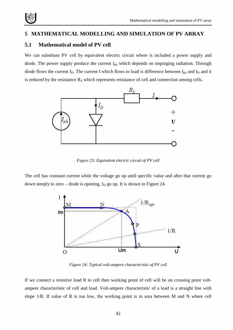


![Orientalism [režim kompatibility]home.zcu.cz/~dkrizek/1EMEA/Orientalism.pdfFour perspectives of Orientalism ’s critique • Orientalism as hegemonic system used to maintain the](https://static.documents.pub/doc/80x56/5b0d0c347f8b9a2f788d2352/orientalism-rezim-kompatibilityhomezcuczdkrizek1emea-perspectives-of-orientalism.jpg)