2009:013 CIV MASTER'S THESIS Modeling of the Interfacial Heat Flow in a Single-belt Casting Simulator Fredrik Nääs Luleå University of Technology MSc Programmes in Engineering Engineering Physics Department of Applied Physics and Mechanical Engineering Division of Physics 2009:013 CIV - ISSN: 1402-1617 - ISRN: LTU-EX--09/013--SE
Transcript
2009:013 CIV
M A S T E R ' S T H E S I S
Modeling of the Interfacial Heat Flowin a Single-belt Casting Simulator
Fredrik Nääs
Luleå University of Technology
MSc Programmes in Engineering Engineering Physics
Department of Applied Physics and Mechanical EngineeringDivision of Physics
Preface This thesis is the final project for the Master of Science in Engineering Physics at Luleå University of Technology. A substantial part of the work has been performed at Novelis Global Technology Centre, NGTC, in Ontario, Canada. I would like to thank my supervisors Dr. Peyman Ashtari and Dr. Kevin Gatenby for their interest in my work to develop the heat-flow model. I would also like to thank Mr. Peter Wales and Mr. Rick Lees for their support in my work to improve the temperature measurements and producing the nose pieces used in the experiments. Finally, I appreciate the time spent and interest shown by my examiner at the university, Prof. Sverker Fredriksson. Luleå, February 2009 Fredrik Nääs
ii
iii
Abstract
Strip casting is a common, low-cost method to cast thin aluminum sheets at gauges close to the final product gauge. Since this process involves fewer steps than traditionally casting methods, the manufacturing time for aluminum products is reduced considerably. Usually, when surface defects occur during the casting process, the slab is scalped. Since it is impractical to scalp a sheet, the slab should contain a minimal amount of surface defects. To achieve this, it is important to understand the effect of different processing variables that occur in the casting procedure. The use of a pilot-scale belt-caster for research is expensive, and therefore, a single-belt casting simulator has been constructed. The aim is to study a broad range of casting conditions and the parameters that affect the surface quality and the underlying microstructure in the twin-belt casting process. Running experiments on the simulator also reduces the costs considerably compared to full scale twin-belt casting experiments. To achieve a sensible simulation, the conditions should be as identical as possible to a twin-belt caster. One of the most crucial factors is the heat-flow occurring in the interface between the solidifying metal and its surroundings. This flow is hard to measure. Therefore, a model for interfacial flow calculations was created. The model was developed in Matlab and Abaqus/CAE. Abaqus/CAE could not compute the desired heat-flow automatically, but was used as a control device for the created algorithm. It was showed that the accuracy of the heat-flow computed with the Matlab algorithm was good. However, many of the cast experiments suffered of measurement errors and unacceptable surface quality. In order to use the belt casting simulator for more advanced experiments, these issues must first be solved.
1.3 Aim of the thesis ....................................................................................................... 5 2 Experimental procedure and equipment ...................................................................... 7
2.1 The casting experiments............................................................................................ 7 2.2 The nosepiece ............................................................................................................ 8 2.3 The substrate ............................................................................................................. 9 2.4 Parting agent............................................................................................................ 10 2.5 Temperature measurements..................................................................................... 11 2.5 Measurement errors................................................................................................. 12
3 Theory ............................................................................................................................ 15 3.1 History of partial differential equations .................................................................. 15 3.2 Properties of partial differential equations .............................................................. 15 3.3 The continuity equation........................................................................................... 17 3.4 The heat equation .................................................................................................... 19 3.5 Numerical solutions of the heat equation ................................................................ 20
3.5.1 Finite differences.............................................................................................. 20 3.5.2 Stability ............................................................................................................ 23 3.5.3 Boundary-value problems for explicit methods ............................................... 24 3.5.4 The Crank-Nicholson implicit method............................................................. 25 3.5.6 Boundary value problems for the Crank-Nicholson implicit method .............. 27
4 The model....................................................................................................................... 29 4.1 Defining the equation .............................................................................................. 29 4.2 The forward difference method............................................................................... 31 4.3 The Crank-Nicholson method ................................................................................. 33 4.4 Investigations of algorithm parameters ................................................................... 36
4.4.1 Time interval, ∆t............................................................................................... 36 4.4.2 Mesh size, h...................................................................................................... 38 4.4.3 Initial guess and matching condition................................................................ 39
Novelis is the world’s largest aluminum rolled products company. It started operations on January 6, 2005 as the spin-off of Alcan Inc.’s (Aluminum company of Canada Limited) aluminum rolled products business. With 38 operating facilities in twelve countries and more than 13,000 employees, Novelis Inc. provides flat rolled aluminum products throughout Asia, Europe, North America and South America. The company supplies aluminum sheet products to beverage and food cans, construction and industrial products and to the automotive and transportation industry. Novelis is also the world’s largest recycler of aluminum beverage cans and recycles annually more than 36 billion used cans. The main purpose of the spin-off from Alcan was to carry on most of the aluminum rolled products business operated by Alcan with the approach to transform new ideas to practical product solutions. The main part of the research takes place at the Novelis Global Technology Center in Kingston (Ontario, Canada) where the work is focused on aluminum-fabricated products, simulations, material performance, and surface treatment.
1.2 Aluminum
Aluminum is the most abundant metal in the earth’s crust and the third most plentiful element after oxygen and silicon. It was first discovered in the 18th century, but it was not until the end of the 19th century aluminum became a commercial product. When the metal was shown on the world fair in Paris 1855, it was considered more expensive than gold [1]. The first commercial applications of aluminum were products like mirror frames and serving trays. Today, the areas of use have grown remarkably and almost every aspect of the modern life is directly or indirectly affected by its use. The metal is used in a broad range of applications, such as beverage containers and cooking utilities, cars and aircraft, and building and construction products. The world production of aluminum has been constantly growing since the metal was discovered. In the early 20th century the world production was approximately 7000 tons annually and in 1970 the yearly production was 9,600,000 tons. Today, the world production is over 25,000,000 tons annually with a constant increasing demand world-wide.
Aluminum is a very versatile metal. It can be developed to fit a broad range of demands and a wide number of alloy compositions are commonly recognized. Some of the most important properties of aluminum are low weight versus strength, fabricability, and corrosion resistance. Packaging
Aluminum is an ideal material for packaging. The metal has light weight and is recyclable, and together with its formability it has superior barrier qualities. Its optical properties help to catch the eye of the consumer, which help manufacturers of packaging to add value to their products. Building and construction
Architects have been enjoying the versatility of aluminum for over 60 years. It has been used to create smooth lines, precise edges and undulating surfaces on every type of construction, from company headquarters to public buildings, from residential buildings to works of art. Closures
Aluminum closures, for example automotive-closures, are one of the most cost effective means of mass reduction available today, and the automotive market is the aluminum industry’s fastest growing market. People want more fuel-efficient cars that are easier on the environment, but without sacrificing safety, comfort and performance. Today’s hood applications, for example, save up to 50% mass over their steel counterparts. Furthermore,
aluminum hoods can be produced at the same rate as their steel counterparts and provide equal or superior denting performance. Aluminum alloys also offer high strength, along with corrosion resistance and good formability. Several auto manufacturers (for example BMW and Cadillac) already use aluminum hoods in some of their models.
1.2.2 Aluminum production
Aluminum is mainly refined from bauxite. The bauxite is washed and dissolved in caustic soda (sodium hydroxide) at high pressure and temperature. The resulting liquid contains a solution of sodium aluminate and undissolved bauxite. After washing, the undissolved bauxite sinks to the bottom of the tank and is removed from the process. The sodium aluminate solution is pumped into another container and pure aluminum oxide (alumina) is added to seed the precipitation of aluminum oxide particles as the fluid cools. These particles sink and are collected at the bottom of the container resulting in a white powder with pure alumina. The production of aluminum from aluminum oxide is based on the Hall-Hérolut process and has not been changed much since aluminum became a commercial product in the early 20th century. The method is very energy consuming, but alternative methods have been found less viable and from both economical and ecological perspectives. In the Hall-Hérolut process, the alumina is dissolved in a cryolite bath and electrolyzed. The separated metal is then periodically removed and transferred to casting facilities, where ingots are produced [2].
1.2.3 Continuous casting
Casting of the ingots can be a time consuming and rather expensive process. Large mechanical equipment with high construction and operational costs are necessary to brake down the ingots closer to the desired product gauge. To reduce these costs, continuous casting procedures have been developed. This is a common, low-cost method to cast thin aluminum sheets at gauges closer to the final product gauge. Since this process involves fewer steps, the manufacturing time for aluminum products is reduced considerably. One common technique for continuous casting of aluminum is the Hazelett caster. In this process, molten metal is introduced between two metal belts. These belts can be seen as conveyer belts onto which the metal is solidifying. The belt material usually consists of copper or steel with a carefully predetermined surface roughness. The metal is solidified by water, which is circulated at high velocity on the opposite side of the conveyer belt. The produced strip has a thickness of about 18-50 mm and is often delivered directly to a nearby rolling mill for further refinement.
4
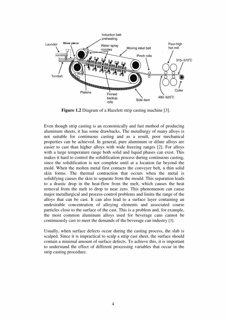
Figure 1.2 Diagram of a Hazelett strip casting machine [3].
Even though strip casting is an economically and fast method of producing aluminum sheets, it has some drawbacks. The metallurgy of many alloys is not suitable for continuous casting and as a result, poor mechanical properties can be achieved. In general, pure aluminum or dilute alloys are easier to cast than higher alloys with wide freezing ranges [2]. For alloys with a large temperature range both solid and liquid phases can exist. This makes it hard to control the solidification process during continuous casting, since the solidification is not complete until at a location far beyond the mold. When the molten metal first contacts the conveyer belt, a thin solid skin forms. The thermal contraction that occurs when the metal is solidifying causes the skin to separate from the mould. This separation leads to a drastic drop in the heat-flow from the melt, which causes the heat removal from the melt to drop to near zero. This phenomenon can cause major metallurgical and process-control problems and limits the range of the alloys that can be cast. It can also lead to a surface layer containing an undesirable concentration of alloying elements and associated coarse particles close to the surface of the cast. This is a problem and, for example, the most common aluminum alloys used for beverage cans cannot be continuously cast to meet the demands of the beverage can industry [3].
Usually, when surface defects occur during the casting process, the slab is scalped. Since it is impractical to scalp a strip cast sheet, the surface should contain a minimal amount of surface defects. To achieve this, it is important to understand the effect of different processing variables that occur in the strip casting procedure.
5
1.3 Aim of the thesis
Continuous strip-casting is a process driven by economics. In order to produce strip cast products, the production must be cheaper than the current method. Traditionally, strip casting has been used in simple alloy systems where there are modest requirements for the final products. Ongoing research of the continuous strip casting technique leads to consequential improvements of the technique and allows wider ranges of alloys to be cast. Since strip casting is a fast and relatively cost-efficient method and there is a high interest in the possibility to use the technique to produce higher value products, such as automotive sheets and beverage container stocks. The use of a pilot scale belt-caster for research is expensive. Relatively big volumes of aluminum must be cast at every experiment and the apparatus takes a lot of manpower to operate. Therefore, a single-belt casting simulator has been constructed. The simulator makes it possible to study a broad range of casting conditions, and most of the parameters affecting the surface quality and the underlying microstructure in the twin belt casting process can be studied. Some of the parameters that can be investigated are parting agents, alloying elements, grain refiners, substrate roughness and material, casting speed, and nose piece design. To achieve a sensible simulation, the casting conditions should be as identical as possible to a twin-belt caster. One of the most crucial factors is the heat-flow occurring in the interface between the solidifying metal and its surroundings. The aim of this thesis is to create a model for interfacial heat-flow calculations and to investigate if the single-belt casting simulator can be used for simple experiments instead of a pilot scale belt caster.
6
7
2 Experimental procedure and equipment
The constructed simulator consisted of a horizontally moving plate called substrate, an electric stepper motor to move the substrate, and a static fixed nosepiece. The construction of the casting simulator was intentionally made simple with few moving parts and simple geometrics to avoid failure during the experiments. All parts of the device were made to imitate the parts in a full-scale belt caster. During the experiments, the stepper motor had its acceleration and speed controlled by a computer, and the substrate was held at a constant velocity of 0.1 m/s. An induction furnace was used to melt the aluminum alloys. The different alloys used in the experiment are from the 1XXX- and 5XXX-series. The content of the alloys is given in Table 2.1
Cast number Alloy type Mg Fe Si
47 5050 1.47 0.30 0.10
48-1 5754 3.33 0.30 0.16
49-1 5182 4.50 0.28 0.09
Cu-1 1XXX - 0.65 0.75
Cu-2 1XXX - 0.65 1.25
Cu-3 1XXX - 0.65 1.50
Fe-1 1XXX - 0.65 0.75
Fe-2 1XXX - 0.65 0.75
Fe-3 1XXX - 0.65 0.75
Table 2.1 Chemical composition of the alloys used (wt %).
2.1 The casting experiments
Two types of casting experiments (static and dynamic tests) were performed to get temperature data for the heat-flow model. Close before the cast, liquid aluminum was poured into the nosepiece. Initially, its exit was blocked by an end block. When the motor started moving the substrate, the liquid metal fed from a 5 mm high gap in the nosepiece onto the substrate as shown in Figure 2.1. Then, the molten metal solidified on the substrate. The second type of casting experiments included static casting tests with a fixed substrate. In these static tests, no nosepiece was used and the liquid aluminum was poured directly onto the substrate where it solidified. During all experiments, temperature data were obtained from a thermocouple mounted in the substrate.
8
Figure 2.1. A single-belt strip-casting simulator, showing (a) the beginning of the casting, and (b) the end of the casting.
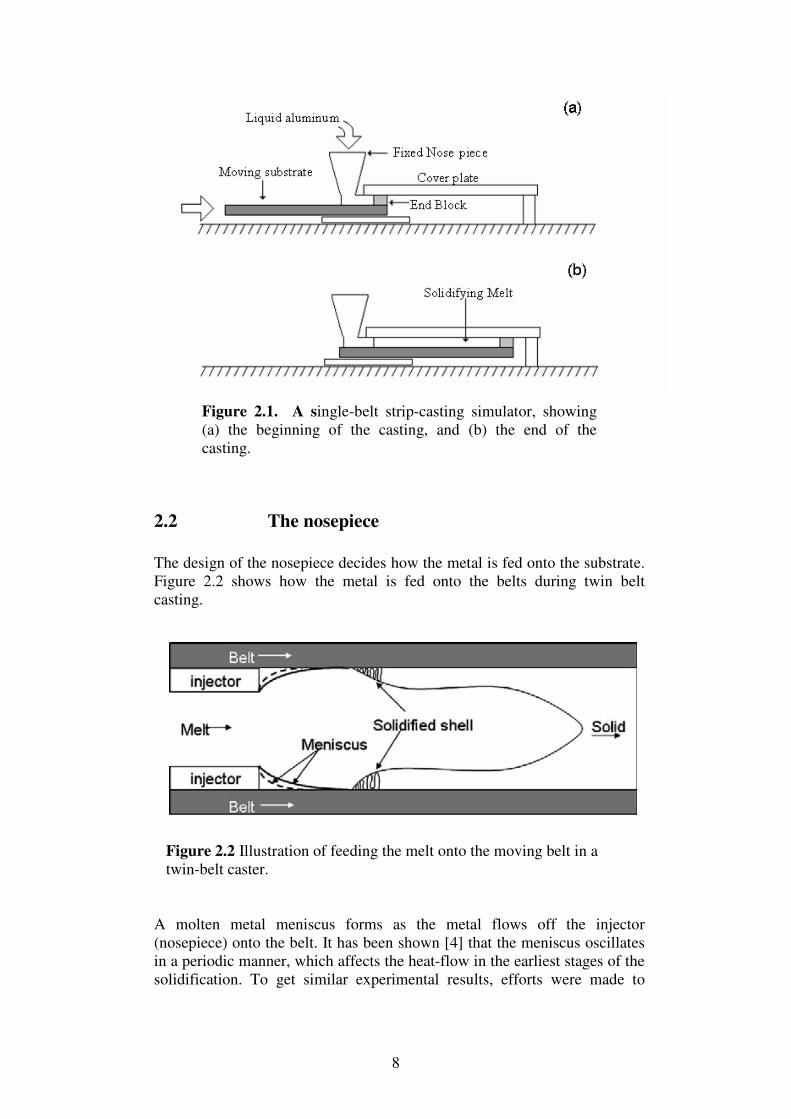
2.2 The nosepiece
The design of the nosepiece decides how the metal is fed onto the substrate. Figure 2.2 shows how the metal is fed onto the belts during twin belt casting.
Figure 2.2 Illustration of feeding the melt onto the moving belt in a twin-belt caster.
A molten metal meniscus forms as the metal flows off the injector (nosepiece) onto the belt. It has been shown [4] that the meniscus oscillates in a periodic manner, which affects the heat-flow in the earliest stages of the solidification. To get similar experimental results, efforts were made to
9
make the nosepiece of the simulator as similar as possible to the nosepiece in a twin-belt caster as possible.
The material for the nosepiece was made of fibrefax paper sheets, coated with silica solution and baked twice in a furnace. The first baking was made with an applied mould in 250 ºC for one hour. To remove all moisture from the sheets, these were baked one more time for one hour at 600 ºC. The top, bottom and side walls of the nosepiece were made from the produced sheets. The tiles where then coated with boron nitride and glued together. After drying, the sides of the nosepiece had to be sanded to fit easily into the belt casting simulator. A cone was then glued on the top of the nosepiece. In the experiments, this cone will contain the liquid metal the seconds before the experiment starts. To remove any moisture, the nosepiece was baked in 150 ºC for at least one hour before it was used.
Figure 2.3 The nosepiece used in the casting experiments.
2.3 The substrate
Two different substrates of low carbon steel and copper were used. In a full scale belt caster, both copper and steel belts are used depending on the alloy to be cast. The substrate in the casting simulator is meant to imitate this belt. Since copper and steel have quite different thermal properties, the heat transfer is expected to show significantly different values depending on the substrate material used for the experiment. It is also known that the substrate roughness plays an important role for the rate of heat-flow and the cast results. Therefore, the roughness on the substrate used in the experiments was chosen to match commonly used belts in a regular strip caster.
10
The copper substrate was mill-finished with an average roughness of 0.80 µm and the steel substrate was shot blasted with an average roughness of 5.64 µm. Table 2.2 shows the thermal properties of the two substrates.
Substrate material C (J/kg·K) k (W/m·K) ρ (kg/m3) Ra (µm)
Steel 486 51.9 7870 5.6
Copper 385 385 8960 0.8
Table 2.2 Thermal and physical properties of the substrates. C is the specific heat, k is the thermal conductivity, ρ is the density, and Ra is the roughness of the substrate surface.
2.4 Parting agent
Different cooling regimens were applied with different substrate preheating temperatures and by applying a parting agent consisting of an oil-mixture. The agent was sprayed on the substrate while it was moving with a constant speed of 0.1 m/s, and the quantity of the applied parting agent was controlled by a screw on the back of the spray gun (see Figure 2.4).
Figure 2.4 The spray gun.
Too much or too little applied parting-agent can lead to bad results of the casting experiments. Therefore, efforts were made to apply an even layer of paring agent on the substrate surface. The applied amount of agent was determined by putting thin aluminum sheets on the substrate and then measuring their weight before and after spraying. The best result with an even applied layer over the entire surface was achieved when the screw of the spray gun was turned 2.5 rounds from its end position. The results from these experiments are shown in table 2.3. In order to make sure that no parting agent was left after the cast, the remaining oil was removed from the substrate with a blow torch and the substrate surface was cleaned with acetone.
11
Weight before spraying (g)
Weight after spraying (g)
Number of turns of the screw
Applied amount (g/m
2)
4.7725 4.7738 2.5 0.20
4.7385 4.7398 2.5 0.20
4.7724 4.7753 3 0.45
4.7679 4.7708 3 0.45
4.7352 4.7379 3 0.42
Table 2.3 Applied amount of parting agent.
2.5 Temperature measurements
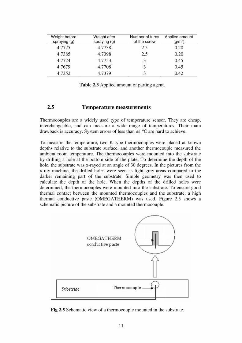
Thermocouples are a widely used type of temperature sensor. They are cheap, interchangeable, and can measure a wide range of temperatures. Their main drawback is accuracy. System errors of less than ±1 ºC are hard to achieve. To measure the temperature, two K-type thermocouples were placed at known depths relative to the substrate surface, and another thermocouple measured the ambient room temperature. The thermocouples were mounted into the substrate by drilling a hole at the bottom side of the plate. To determine the depth of the hole, the substrate was x-rayed at an angle of 30 degrees. In the pictures from the x-ray machine, the drilled holes were seen as light grey areas compared to the darker remaining part of the substrate. Simple geometry was then used to calculate the depth of the hole. When the depths of the drilled holes were determined, the thermocouples were mounted into the substrate. To ensure good thermal contact between the mounted thermocouples and the substrate, a high thermal conductive paste (OMEGATHERM) was used. Figure 2.5 shows a schematic picture of the substrate and a mounted thermocouple.
Fig 2.5 Schematic view of a thermocouple mounted in the substrate.
12
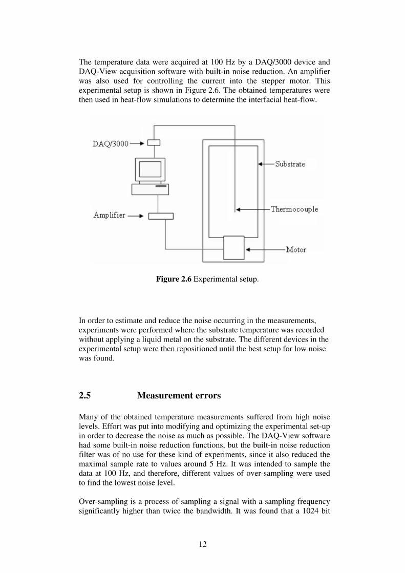
The temperature data were acquired at 100 Hz by a DAQ/3000 device and DAQ-View acquisition software with built-in noise reduction. An amplifier was also used for controlling the current into the stepper motor. This experimental setup is shown in Figure 2.6. The obtained temperatures were then used in heat-flow simulations to determine the interfacial heat-flow.
Figure 2.6 Experimental setup.
In order to estimate and reduce the noise occurring in the measurements, experiments were performed where the substrate temperature was recorded without applying a liquid metal on the substrate. The different devices in the experimental setup were then repositioned until the best setup for low noise was found.
2.5 Measurement errors
Many of the obtained temperature measurements suffered from high noise levels. Effort was put into modifying and optimizing the experimental set-up in order to decrease the noise as much as possible. The DAQ-View software had some built-in noise reduction functions, but the built-in noise reduction filter was of no use for these kind of experiments, since it also reduced the maximal sample rate to values around 5 Hz. It was intended to sample the data at 100 Hz, and therefore, different values of over-sampling were used to find the lowest noise level. Over-sampling is a process of sampling a signal with a sampling frequency significantly higher than twice the bandwidth. It was found that a 1024 bit
13
over-sampled temperature measurement gave the lowest noise at a sample rate of 100 Hz. High bit-rates gave less noise but also decreased the allowed maximal sample frequency. The effect on the noise level caused by the induction furnace and stepper motor was also investigated. It was found that the induction furnace had negligible effect on the measured noise levels. However, with the stepper motor running, the noise increased considerably. Figure 2.7 shows a typical noise-plot from these experiments.
Figure 2.7 Lowest measured noise. The temperature data is sampled at 100 Hz with 1024 bit over-sampling.
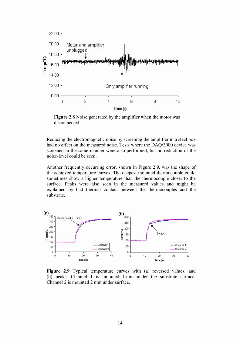
In order to tell if the occurred noise was generated by the amplifier or directly from the stepper motor, experiments with the amplifier connected, but the stepper motor disconnected were performed. As seen in Figure 2.8, the measured noise increased when the amplifier was turned on, but it automatically stopped generating current when it detected that the motor was disconnected. Therefore, it was hard to tell which one of the two devices that caused the high noise seen in the measurements.
14
Figure 2.8 Noise generated by the amplifier when the motor was disconnected.
Reducing the electromagnetic noise by screening the amplifier in a steel box had no effect on the measured noise. Tests where the DAQ/3000 device was screened in the same manner were also performed, but no reduction of the noise-level could be seen. Another frequently occurring error, shown in Figure 2.9, was the shape of the achieved temperature curves. The deepest mounted thermocouple could sometimes show a higher temperature than the thermocouple closer to the surface. Peaks were also seen in the measured values and might be explained by bad thermal contact between the thermocouples and the substrate.
Figure 2.9 Typical temperature curves with (a) reversed values, and (b) peaks. Channel 1 is mounted 1 mm under the substrate surface. Channel 2 is mounted 2 mm under surface.
15
3 Theory
3.1 History of partial differential equations
Partial differential equations were not consciously created as a subject in mathematics until the 18th century when ordinary differential equations failed to describe the physical principles being studied. Some of the major names of mathematics have contributed greatly to the subject. Leonard Euler and Joseph-Louis Lagrange studied waves on strings, and Joseph Fourier made his famous work on series expansions for the heat equation, which is studied in this thesis. Many of the greatest advances in modern science have been based on the discoveries of the underlying mathematical theories of partial differential equations. James Clerk Maxwell created Maxwell’s equations for electromagnetic theory. His work gave solutions for problems in radio-wave propagation, the diffraction of light and the development of X-rays. In fluid dynamics, the Navier-Stokes equations are the basics of numerical calculations used in widely spread areas such as weather-forecasting and aircraft design. The Schrödinger equation for quantum mechanical processes is yet another example based on the underlying theory of partial differential equations. The development of numerical solutions of partial differential equations has been heavily influenced by the development of high-speed computing machines. In the mid 20th century, the cold war was instrumental in forcing hand-worked numerical solutions to problems like blast waves from atomic bombs. A large number of electro-mechanical machines were used. They were controlled by a programmer, and much effort was required to check for human errors in the process. When more reliable and faster computers were developed, more complex partial differential equations could be solved numerically [5].
3.2 Properties of partial differential equations
A partial differential equation (PDE) can be described as a differential equation with more than one differentiable variable. One example is
xue
dy
du
dx
du
x
u=
−
∂
∂sin
2
2
. (3.1)
The highest derivative in the equation defines its order. For example, Equation 3.1 is of order two. One useful classification of partial differential equations is linearity. If two different solutions, u1 and u2, have been found to a partial differential equation, it is said to be linear if the sum of u1 and u2 also is a solution to the equation. This implies that if a function u and all
16
partial derivatives occur as linear expressions, the equation is linear. Equation (3.2) below is linear, whereas the previous equation (3.1) is not:
xyyx
ue
x
uxy
yx cos2
2
2
=∂∂
∂−
∂
∂ − . (3.2)
The coefficients of a linear partial differential equation can be functions of x and y, but not functions of u. There are three kinds of partial differential equations, hyperbolic, parabolic, and elliptic equations. Consider the second order PDE:
gyx
uC
y
uB
x
uA =
∂∂
∂+
∂
∂+
∂
∂ 2
2
2
2
2
. (3.3)
The equation is said to be hyperbolic if C2
- 4AB > 0. A hyperbolic equation will behave like enduring disturbances that expands. One common hyperbolic PDE is the wave-equation. If C2
- 4AB < 0, the equation is said to be elliptic. An example of an elliptic PDE is Poisson’s equation. If C
2 - 4AB = 0, the equation is parabolic and has the property to level out
fluctuations. If the coefficients A, B, and C are non constant, the equation can be of one type in a specified interval and of another type in another interval (e.g. elliptic in 0 < x < 1 and hyperbolic for all other values of x) [6]. The equation considered in this thesis is the linear, one dimensional, parabolic heat equation:
fx
ua
t
u=
∂
∂−
∂
∂2
2
, (3.4)
which can be derived from the continuity equation.
17
3.3 The continuity equation
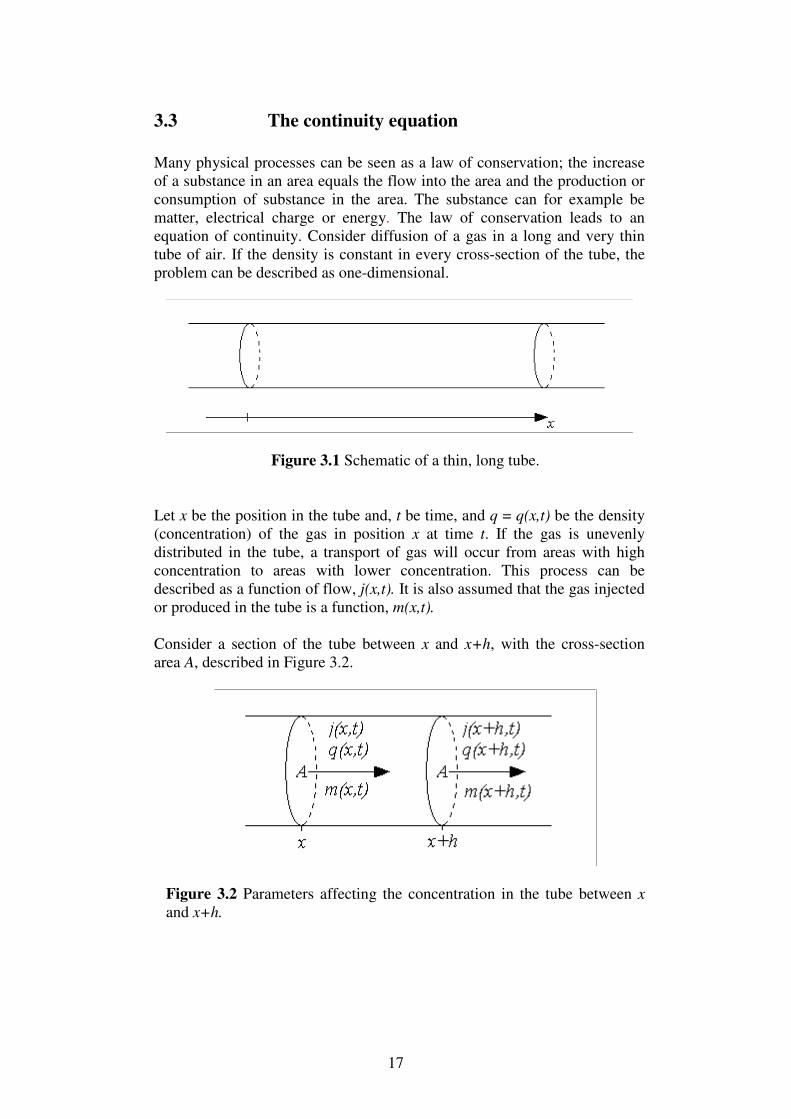
Many physical processes can be seen as a law of conservation; the increase of a substance in an area equals the flow into the area and the production or consumption of substance in the area. The substance can for example be matter, electrical charge or energy. The law of conservation leads to an equation of continuity. Consider diffusion of a gas in a long and very thin tube of air. If the density is constant in every cross-section of the tube, the problem can be described as one-dimensional.
Figure 3.1 Schematic of a thin, long tube.
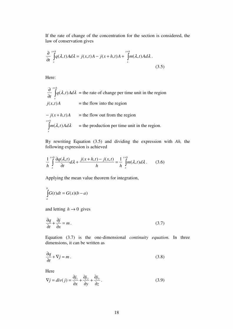
Let x be the position in the tube and, t be time, and q = q(x,t) be the density (concentration) of the gas in position x at time t. If the gas is unevenly distributed in the tube, a transport of gas will occur from areas with high concentration to areas with lower concentration. This process can be described as a function of flow, j(x,t). It is also assumed that the gas injected or produced in the tube is a function, m(x,t). Consider a section of the tube between x and x+h, with the cross-section area A, described in Figure 3.2.
Figure 3.2 Parameters affecting the concentration in the tube between x
and x+h.
18
If the rate of change of the concentration for the section is considered, the law of conservation gives
∫∫++
++−=∂
∂hx
x
hx
x
AdtmAthxjAtxjdAtqt
λλλλ ),(),(),(),( .
(3.5) Here:
λλ dAtqt
hx
x
∫+
∂
∂),( = the rate of change per time unit in the region
Atxj ),( = the flow into the region
Athxj ),( +− = the flow out from the region
∫+hx
x
Adtm λλ ),( = the production per time unit in the region.
By rewriting Equation (3.5) and dividing the expression with Ah, the following expression is achieved
∫∫++
=−+
+∂
∂hx
x
hx
x
dtmhh
txjthxjd
t
tq
hλλλ
λ),(
1),(),(),(1. (3.6)
Applying the mean value theorem for integration,
∫ −=b
a
abxGdttG ))(()(
and letting 0→h gives
mx
j
t
q=
∂
∂+
∂
∂. (3.7)
Equation (3.7) is the one-dimensional continuity equation. In three dimensions, it can be written as
mjt
q=∇+
∂
∂. (3.8)
Here
z
j
y
j
x
jjdivj
∂
∂+
∂
∂+
∂
∂==∇ 321)( . (3.9)
19
A continuity equation is a general equation that describes the conservative transport of some kind of quantity. Since mass, energy, momentum, and other natural quantities are conserved, a vast variety of physical processes may be described by continuity equations. In the following section, the heat equation will be derived from the tree-dimensional continuity equation (3.8).
3.4 The heat equation
Heat can be defined as the form of energy that is transferred across the boundary of a system with a given temperature to its surroundings with a lower or higher temperature. This transfer takes place solely because of the temperature difference between the two systems. If an arbitrary, three-dimensional isotropic body with a given temperature is affected by its warmer surroundings, energy transfer will take place between the two systems. In this case, the continuity equation (3.8) governs since energy will be conserved in the body. Let q, j and m be functions of the body, where
q(x,y,z,t) = heat or energy density (J/m3) j(x,y,z,t ) = heat-flow density (J/m2s) m(x,y,z,t) = added heat per volume and time unit (J/m3s). Let us consider the properties of the participating parameters q, j, and m in a heat conductive body. When the warm surrounding affects the cool body, a heat-flow will occur in the interface between the two systems. In isotropic materials, this heat-flow can be described by Fourier’s law j = - k grad(T), (3.10)
where k is the thermal conductivity (W/m·K) of the body. The minus sign in the equation gives a direction of the heat transfer from a higher temperature to a lower temperature region. Furthermore, the size of the heat-flow is proportional to the temperature change per length unit in this direction. At small changes of the temperature, the change of energy density dq, can be assumed to be proportional to the temperature change dT according to Newton’s law of cooling,
dTcdq ρ= , (3.11)
where ρ is density (kg/m3) and c is the specific heat capacity (J/kg·K). When we combine Newton’s law of cooling (3.11) and Fourier’s law (3.10) with the continuity equation (3.8), we achieve the three-dimensional heat equation below (3.12):
20
mgradTkdivt
TC =⋅−
∂
∂)(ρ , (3.12)
which also can be written as
mTkt
TC =∇⋅⋅∇−
∂
∂)(ρ . (3.13)
For a unique solution, one must also specify the initial values u(x,y,z,0), and the boundary conditions to the equation. There are two general types of boundary conditions for the heat equation, Dirichlet and Neumann conditions. A Dirichlet condition corresponds to boundaries held at given temperatures, while Neumann conditions correspond to given heat-flow rates on the boundary (e.g., insulation). A third condition, the Robin condition, corresponds to imperfect insulation and can be said to be a combination of Dirichlet and Neumann conditions. The heat equation describes the temperature for a function u, at a given location (x, y, z) in a specified region. The equation is used to determine the temperature change of a function u over time. One interesting property of the heat equation is that the maximal temperature always comes earlier in time than the region studied, or that the maximal temperature is at the edge of the region. This might seem obvious since heat can be transported into a region but not be created from nothing. However, this is a general property of a parabolic, partial differential equation and is a basis for the maximal principle for the heat equation [7].
3.5 Numerical solutions of the heat equation
3.5.1 Finite differences
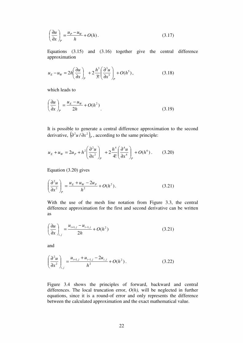
The finite differences method is a numerical method of solving partial differential equations. By approximating the full partial differential equation with sets of algebraic equations, a numerical approach for solving the problem is achieved. The result is that partial derivatives are replaced by relationships between the function values at nodal points of a grid system.
21
Figure 3.3. A typical grid system.
Consider a typical grid system shown in Figure 3.3. A mesh with a constant increment h in the horizontal direction and a constant increment k in the vertical direction is chosen. Using Taylor series in one variable, keeping the other variable fixed gives
⋅⋅⋅+
∂
∂+
∂
∂+
∂
∂+
∂
∂+=
PPPP
pEx
uh
x
uh
x
uh
x
uhuu
4
44
3
33
2
22
!4!3!2
(3.14)
and
⋅⋅⋅+
∂
∂+
∂
∂−
∂
∂+
∂
∂−=
PPPP
pWx
uh
x
uh
x
uh
x
uhuu
4
44
3
33
2
22
!4!3!2.
(3.15)
Equation (3.14) gives the forward difference approximation
)(hOh
uu
x
u PE
P
+−
=
∂
∂. (3.16)
The reminder term of O(h) is called the local truncation error. It is a round-off error and represents the difference between the calculated approximation and the exact mathematical value. Here, it is determined by the remaining terms in the Taylor series expansion.
Similarly, Equation (3.15) gives the backward difference approximation
22
)(hOh
uu
x
u WP
P
+−
=
∂
∂. (3.17)
Equations (3.15) and (3.16) together give the central difference approximation
)(!3
22 5
3
33
hOx
uh
x
uhuu
PP
WE +
∂
∂+
∂
∂=− , (3.18)
which leads to
)(2
2hO
h
uu
x
u WE
P
+−
=
∂
∂
. (3.19)
It is possible to generate a central difference approximation to the second
derivative, ( )P
xu22 / ∂∂ , according to the same principle:
)(!4
22 6
4
44
2
22
hOx
uh
x
uhuuu
PP
PWE +
∂
∂+
∂
∂+=+ . (3.20)
Equation (3.20) gives
)(2 2
22
2
hOh
uuu
x
u PWE
P
+−+
=
∂
∂. (3.21)
With the use of the mesh line notation from Figure 3.3, the central difference approximation for the first and second derivative can be written as
)(2
2,1,1
,
hOh
uu
x
u jiji
ji
+−
=
∂
∂ −+ (3.21)
and
)(2
2
2
,,1,1
,
2
2
hOh
uuu
x
u jijiji
ji
+−+
=
∂
∂ −+. (3.22)
Figure 3.4 shows the principles of forward, backward and central differences. The local truncation error, O(h), will be neglected in further equations, since it is a round-of error and only represents the difference between the calculated approximation and the exact mathematical value.
23
Figure 3.4 The (a) backward, (b) forward, and (c) central difference approximations of the function f(x) at point i.
3.5.2 Stability
Consider the one-dimensional parabolic equation
2
2
dx
u
t
u ∂=
∂
∂. (3.23)
A grid increment k and space increment h are used. A forward difference
approximation is used for tu ∂∂ / and a central difference approximation is
used for 22 / xu ∂∂ :
2
,,1,1,1, 2
h
uuu
k
uu jijijijiji −+=
− −++. (3.24)
If r = k/h
2 the equation becomes
jijijiji uruuru ,1,1,1, )21()( −++= +−+ . (3.25)
The left side of the equation contains the unknown value of the next time-step and the right side describes the known values of the previous time-step. In this method, no systems of equations have to be solved. This is called an explicit method. The right side of Equation (3.25) expresses a weighted arithmetic mean value of ui,j+1, ui,j, and ui,j-1. If the method is stable, the calculated value of ui+1,j lies somewhere in the interval between the three values of the previous time step. In Equation (3.25) this is true if all coefficients are positive, which corresponds to
2
10 ≤< r . (3.26)
Since r = k/h
2 Equation (3.26) implies that the step size k must be
24
2
2h
k ≤ , (3.27)
if stability is to be maintained [6]. According to Lax equivalence theorem, a stable solution is also convergent [8].
3.5.3 Boundary-value problems for explicit methods
At interior points, there is no problem to approximate derivatives, but problems can occur at the boundaries. For Dirichlet conditions, u is directly specified at the boundaries and therefore, Dirichlet boundary conditions rarely cause problems. For Neumann conditions however, derivatives of u are given, and the representation of the partial differential equation is required at the boundary. Consider the boundary condition (∂u/∂x) = g, which corresponds to a constant heat-flow on the boundary. A problem occurs, since there are no further points to use to describe the derivative. One way to deal with this is to invent a fictitious point E’. With this point introduced, the derivative (∂u/∂x) at the boundary becomes
gh
uu WE =−
2
' . (3.28)
This is schematically shown in Figure 3.5.
Figure 3.5 A fictitious point E’ is used to describe the derivative at the boundary point P.
25
The central difference approximation of 22 / xu ∂∂ at the boundary is
2
'
2
2 2
h
uuu
x
u PWE
P
−+=
∂
∂. (3.29)
From Equation (3.28) we see that uE’ can be written as
WE uhgu += 2' . (3.30)
Equation (3.29) then becomes
22
2 22
h
uuuhg
x
u PWW
P
−++=
∂
∂, (3.31)
which can be rewritten as
22
2 )(2
h
uuhg
x
u PW
P
−+=
∂
∂. (3.32)
With the use of Equation (3.32) for the first and last node in the system, it is possible to create a finite difference approximation to second-order partial differential equations with boundary conditions of Neumann type.
3.5.4 The Crank-Nicholson implicit method
The explicit method has the drawback that the step size k must be small if
stability is to be maintained. In the Crank-Nicholson method, 22 / xu ∂∂ is replaced by the mean of its finite difference representations at the j:th and (j+1):th time levels. This method is stable for all finite values of r [5]. For
2
2
dx
u
t
u ∂=
∂
∂ (3.33)
the Crank-Nicholson scheme is
−++
−+=
− ++−++−++
2
1,1,11,1
2
,,1,1,1, 22
2
1
h
uuu
h
uuu
k
uu jijijijijijijiji,
(3.34) where an average is taken to represent the second-order derivative. This equation can be rewritten as
The right-hand side of the equation is known, but the left-hand side involves three successive unknown values. Equation (3.35) leads to a tridiagonal set of linear equations, which have to be solved at each time level. A method where the calculation of unknown nodal values requires the solution of a set of simultaneous equations is called an implicit method. In matrix-form, Equation (3.35) is written as
•
−
−
−
−
=
•
+−
−+−
−+−
−+
−
−
+−
+−
+
+
jn
jn
j
j
jn
jn
j
j
u
u
u
u
rr
rrr
rrr
rr
u
u
u
u
rr
rrr
rrr
rr
,1
,2
,2
,1
1,1
1,2
1,2
1,1
22
22
22
22
22
22
22
22
MOOOMOOO ,
(3.36)
or in compact form
[ ] [ ] jnjn urTIurTI ⋅+=⋅− −+− 111 22 . (3.37)
Here
−
−
−
−
=−
21
121
121
12
1 OOOnT .
To solve the unknown value at the next time level, Equation (3.37) is written as
[ ] [ ] jnnj urTIrTIu ⋅+⋅−= −
−
−+ 1
1
11 22 . (3.38)
This is the Crank-Nicholson implicit scheme.
27
3.5.6 Boundary value problems for the Crank-Nicholson
implicit method
As for the explicit method, boundary conditions have to be defined for the end-points in the system. For Neumann conditions the method is quite similar to the explicit problem. A fictitious point E’ is created to describe
the boundary condition ( ) gxu =∂∂ / . The Crank-Nicholson method is an
implicit method, and therefore, both point E’j and point E’j+1 for the upcoming time step must be defined to describe the boundary conditions. These become
(3.42) In matrix form, the Crank-Nicholson scheme with applied Neumann boundary conditions becomes
⋅−
⋅−
+
•
−
−
−
−
=
•
+−
−+−
−+−
−+
−
−
+−
+−
+
+
rgh
rgh
u
u
u
u
rr
rrr
rrr
rr
u
u
u
u
rr
rrr
rrr
rr
jn
jn
j
j
jn
jn
j
j
4
0
0
4
222
2222
2222
222
222
2222
2222
222
,1
,2
,2
,1
1,1
1,2
1,2
1,1
MMOOOMOOO.
(3.43)
28
29
4 The model
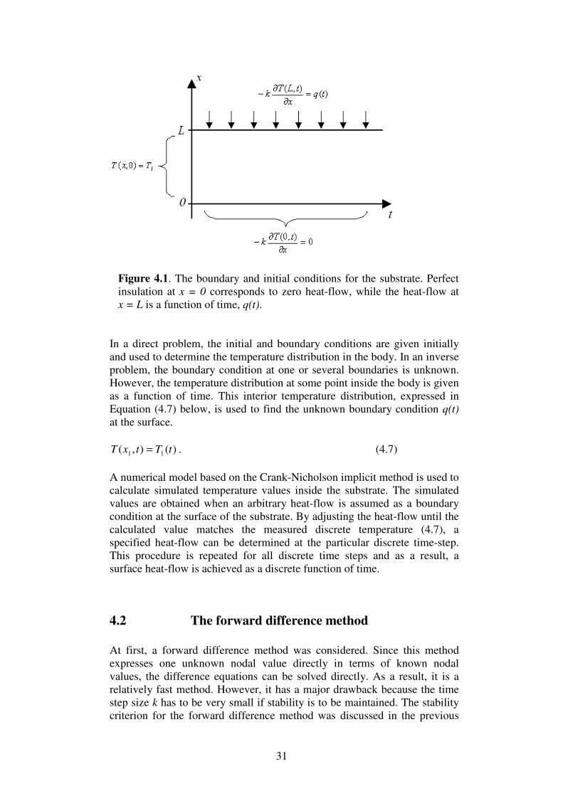
If the heat-flow or the temperature history at the surface of a solid is known as a function of time, the temperature distribution in the body can be found. This is called a direct heat-conduction problem. In many situations it can be difficult to measure the surface temperature or the surface heat-flow of a body. In this thesis, melted aluminum is solidifying on a substrate, and it is desired to find the heat-flow at the interface between the metal and the substrate. This interfacial heat-flow, and the corresponding interfacial temperature, is hard to measure since it is unsuitable to attach a temperature sensor at the surface of the substrate. It is also difficult to know whether the measured temperature of such a sensor registers the temperature of the melt, the temperature of the substrate, or the desired temperature at the thin interface between the substrate and the melt. Therefore, the temperature is measured at an interior location of the substrate, and the surface temperature and heat-flow is calculated from these measurements. This is an inverse heat conduction problem.
4.1 Defining the equation
The starting point for evaluation of the interfacial heat-flow is the heat equation derived in Section 3.4:
mTat
TC =∇⋅⋅∇−
∂
∂)(ρ , (4.1)
where ρ = density (kg/m3), C = specific heat (J/kg·K), a = thermal conductivity (W/m·K), T = temperature (°C), t = time (s), x = vertical position (m). The thermal conductivity is normally called k, but is here named a in order to avoid confusion with the time step size k of the finite difference scheme explained in the previous section. When the melted aluminum hits the substrate, heat will be transferred from the warm liquid metal to the colder substrate as the metal solidifies. This process can be seen as an energy transfer to the substrate due to a heat-flow on the substrate boundary. Since no heat is created in the substrate, the right side of Equation (4.1) is zero. Furthermore, the substrate can be seen as a thin plate, so the longitudinal and latitudinal heat conduction is assumed to be negligible in comparison with the vertical conduction. Equation (4.1) can now be rewritten as
30
02
2
=∂
∂−
∂
∂
x
Ta
t
TCρ . (4.2)
With αρ
=C
a Equation (4.2) becomes
2
2
x
T
t
T
∂
∂=
∂
∂α . (4.3)
In order to make a more simplified model, the density, thermal conductivity, and specific heat are assumed to be temperature independent. It is also assumed that the substrate bottom surface is perfectly insulated. The initial and boundary conditions for Equation (4.3) are expressed by
iTxT =)0,( (4.4)
)(),(
tqqx
tLTa Lx ==
∂
∂− = (4.5)
0),0(
0 ==∂
∂− =xq
x
tTa . (4.6)
The minus sign in boundary condition (4.5) gives a direction of the heat-flow from a higher to a lower temperature region. This heat transfer arises when the temperature difference between the warm, solidifying aluminum cast and the colder substrate is leveled out. It is a transient (time-dependent) process where the cast cools off as a function of time, and as a result, the heat-flow at the substrate surface is also time dependent.
31
Figure 4.1. The boundary and initial conditions for the substrate. Perfect insulation at x = 0 corresponds to zero heat-flow, while the heat-flow at x = L is a function of time, q(t).
In a direct problem, the initial and boundary conditions are given initially and used to determine the temperature distribution in the body. In an inverse problem, the boundary condition at one or several boundaries is unknown. However, the temperature distribution at some point inside the body is given as a function of time. This interior temperature distribution, expressed in Equation (4.7) below, is used to find the unknown boundary condition q(t) at the surface.
)(),( 11 tTtxT = . (4.7)
A numerical model based on the Crank-Nicholson implicit method is used to calculate simulated temperature values inside the substrate. The simulated values are obtained when an arbitrary heat-flow is assumed as a boundary condition at the surface of the substrate. By adjusting the heat-flow until the calculated value matches the measured discrete temperature (4.7), a specified heat-flow can be determined at the particular discrete time-step. This procedure is repeated for all discrete time steps and as a result, a surface heat-flow is achieved as a discrete function of time.
4.2 The forward difference method
At first, a forward difference method was considered. Since this method expresses one unknown nodal value directly in terms of known nodal values, the difference equations can be solved directly. As a result, it is a relatively fast method. However, it has a major drawback because the time step size k has to be very small if stability is to be maintained. The stability criterion for the forward difference method was discussed in the previous
32
section. It states that the time-step size has to be less than half the square of the space step size for a stable solution. The explicit scheme is
)2( ,,1,1,1, jijijijiji uuuruu −++= −++ , (4.8)
where 2
12
≤=h
kr α for a stable solution. This implies that
α2
2h
k ≤ (4.9)
for a stable solution of the equation.
For example, with some typical thermal properties for a steel substrate,α becomes 1.36·10-5 m2/s. If the mesh size is 0.5 mm, the time step must be smaller than 0.0092 seconds for a stable solution. In Figure 4.2 below, two heat simulations are performed with identical input parameters. The left mesh is obtained from a simulation performed with a 0.009 second time-step while the right mesh is from a simulation with a time-step of 0.0095 seconds. It is obvious that the right mesh shows an unstable solution of the solved equation.
Figure 4.2. Two simulations of the heat equation for a thin plate. The plate is insulated at x = 0 and is affected by a constant 1 MW/m2 heat-flow at x = 10 mm. Its initial temperature is 0 ºC.
Since the explicit method is unstable in many situations and the aim is to create a numerical model that does not require too much knowledge about the numerical process, a Crank-Nicholson implicit scheme is used instead of the forward Euler method presented above. The Crank-Nicholson method is stable for all real values of r [5].
33
4.3 The Crank-Nicholson method
Because of the unstable behavior of the explicit finite difference scheme, it was decided to create a model based on the implicit Crank-Nicholson method. This scheme can be written as
(4.10) The right-hand side of the equation is known, but the left-hand side involves three successive unknown values. Equation (4.10) leads to a tridiagonal set of linear equations, which have to be solved at each time level. A method where several unknown future time steps are involved requires to be solved by a system of equations. It is often characterized as an implicit method. In compact form, the Crank-Nicholson implicit scheme (4.10) can be written as
[ ] [ ] jnjn urTIurTI ⋅+=⋅− −+− 111 22 , (4.11)
where
−
−
−
−
=−
21
121
121
12
1 OOOnT .
When the boundary conditions (4.5) and (4.6) are applied, the scheme can be rewritten as
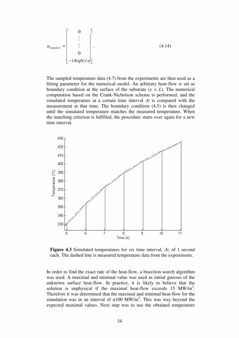
The sampled temperature data (4.7) from the experiments are then used as a fitting parameter for the numerical model. An arbitrary heat-flow is set as boundary condition at the surface of the substrate (x = L). The numerical computation based on the Crank-Nicholson scheme is performed, and the simulated temperature at a certain time interval ∆t is compared with the measurement at that time. The boundary condition (4.5) is then changed until the simulated temperature matches the measured temperature. When the matching criterion is fulfilled, the procedure starts over again for a new time interval.
Figure 4.3 Simulated temperatures for six time interval, ∆t, of 1 second each. The dashed line is measured temperature data from the experiments.
In order to find the exact rate of the heat-flow, a bisection search algorithm was used. A maximal and minimal value was used as initial guesses of the unknown surface heat-flow. In practice, it is likely to believe that the solution is unphysical if the maximal heat-flow exceeds 15 MW/m2. Therefore it was determined that the maximal and minimal heat-flow for the simulation was in an interval of ±100 MW/m2. This was way beyond the expected maximal values. Next step was to use the obtained temperature
35
from the simulation and compare it with the measured temperature from the casting experiments. The heat-flow interval was then repeatedly cut in half until the simulated result matched the experimental measurements within an error range, ε of 0.001 ºC. The obtained heat-flow was then plotted versus time to achieve a heat-flow history, as shown in Figure 4.4.
Figure 4.4 A typical history of the calculated heat-flow from a simulation
It is important to remind that the investigated time interval ∆t is not the same as the time step k used in the basic Crank-Nicholson calculations. The calculated heat-flow is discretely changed for every new time interval, but constant during one specific interval. These time interval can in turn consist of an arbitrary, but constant number of time steps k defined by the finite difference approximation. This is schematically explained in Figure 4.5 below.
Figure 4.5. Schematic of ∆t and k
To avoid misunderstanding, the time step parameter k in the basic Crank-Nicholson method will not be further investigated. This is also due to the fact that it is convenient to keep the time step k equal to the sample rate of the measured values from the experiments. Therefore, k will be constant in all further investigations. The investigated parameters will be the size of the space step h from the finite difference approximation, the time interval ∆t of the heat-flow calculations, and the error range ε, which is used as a fitting parameter between the measured and simulated values.
36
4.4 Investigations of algorithm parameters
4.4.1 Time interval, ∆t
An advantage of this inverse method is its simplicity, which permits easy understanding of the method and the development of the algorithm. A time interval of 0.1 second was usually used in the simulations. This leads to a resolution of 10 Hz for the calculated heat-flow. However, an interesting unstable behavior was detected as ∆t for the heat-flow calculations was made small. A finite difference method is normally more precise and stable as the time step k is made small. This seems to be the opposite case when the heat-flow algorithm is added to the basic finite difference method. As ∆t becomes small in the heat-flow calculations, instability seems to increase. Numerical experiments were performed where the temperature curve from a simulation with a constant heat-flow of 1 MW/m2 was used as a matching variable. The inverse algorithm was then used to calculate this known heat-flow independently. The time interval for the algorithm was changed from 0.5 seconds to 0.01 second and the minimal time interval for stability was investigated. Unstable solutions were achieved for time intervals smaller than 0.02 seconds. It was also detected that when the time interval was big, the error of the heat-flow calculations got smaller. In Figure 4.6, it is clearly shown that, for all stable solutions, the error was most significant in the beginning of the simulations and almost completely damped after approximately 0.5 seconds. The instability phenomenon for small ∆t, seen in Figure 4.6 d, could not be explained. However, since the matching curve was perfectly smooth, there was no influence of noise in the investigations. This could imply that the unstable behavior is related from the heat-flow algorithm and is not significantly affected by surrounding error sources such as noise and measurement errors.
37
Figure 4.6 The result from the inverse algorithm is shown for a time interval of (a) 0.1 second, (b) 0.05 seconds, (c) 0.03 seconds, and (d) 0.01 seconds. The mesh size is set to 0.5 mm in all calculations.
A small ∆t resulted in high noise levels for the calculated surface heat-flow. This phenomenon was easily avoided by increasing the length of the time interval. If a large time interval was used, the final heat-flow curve got smooth but resulted at the same time in too low resolution. This was not wanted. Figure 4.7 below, shows how the heat-flow curve was affected by noise depending on the time interval used.
Figure 4.7 Two heat-flow vs. time curves. The left flow curve is achieved with a 0.25 second time interval, while the right uses an interval of 0.5 seconds.
38
It was concluded that it was impractical to use a time interval smaller than 0.1 second due to the risk of instability in the heat-flow algorithm and high noise levels for the calculated heat-flow curves. The noise levels in the calculated heat-flow could be reduced by filtering the measured temperature curve before using it in the simulations.
4.4.2 Mesh size, h
It was also investigated how the mesh size of the basic Crank-Nicholson algorithm affected the stability and error range in the algorithm. In most finite difference approximations, a smaller mesh size leads to a more precise simulation, but is also more costly in terms of computer capacity. The results from the investigations, presented in Table 4.1, were achieved with a constant surface heat-flow of 1 MW/m2. They show that no clear trend of unstability was detected when the mesh size was changed.
Time interval ∆t (s)
Mesh size h = 0.5 mm
Mesh size h = 0.25 mm
Mesh size h = 0.1 mm
0.50 0.013 0.016 0.016
0.10 0.089 0.102 0.106
0.05 0.126 0.105 0.123
0.03 0.352 0.323 0.307
0.01 Unstable Unstable Unstable
Table 4.1 Maximal error (MW/m2) of the heat-flow calculations with respect to the time interval, ∆t, and mesh size, h.
Figure 4.7 below, shows the calculated heat-flow over a time period of 30 seconds for a transient heat-flow simulation. A time interval of 0.1 second was used in both Figures but the mesh size is changed from 0.5 mm in the right Figure to 0.1 mm in the left. No significant difference can be seen between the two calculations. Considering that the efficiency and speed of the algorithm was greatly decreased with a small mesh, a relatively coarse space step of 0.5 mm was used for all inverse heat-flow calculations.
39
Figure 4.7 Two heat-flow calculations with a time step of 0.5 seconds and a varying mesh size of (a) 0.5 mm and (b) 0.1 mm. The results are almost identical.
4.4.3 Initial guess and matching condition
The bisection algorithm, used to find the appropriate heat-flow for every time interval, is a simple search method. Initial maximal and minimal heat-flows are set as starting points. The interval that forms between these heat-flows is then repeatedly cut in half until the simulated temperature matches a measured temperature within a certain error range, ε. In order to increase the computing speed of the heat-flow algorithm without compromising with accuracy, it was of interest to investigate how different values of ε and the initial heat-flow interval affected the algorithm. It was found that by decreasing or increasing the initial heat-flow interval with a factor 10, the maximal iterations needed to meet the matching condition were changed with approximately 15%. About the same relation was found for the number of iterations when ε was changed with a factor 10. However, a fine matching condition contributed greatly to an increased accuracy of the simulation. The conclusion from these tests was that both the initial maximal and minimal heat-flow and the matching condition affect the number of iterations in the search method. Thereby they affect the speed of the entire algorithm. Since high precision simulations are more important than a fast algorithm, no modifications were made to the initial guess of the heat-flow and the matching condition, ε.
40
Figure 4.8 The number of iterations required to achieve the matching condition for every time interval. In this Figure, the matching condition (ε) is 10-4 and the time interval (∆t) 0.1 second.
4.5 Abaqus/CAE simulations
In order to check if the calculated heat-flow was correct, a commercial software, Abaqus/CAE, was used. The advantage of Abaqus/CAE is the ease with which a diverse range of physical problems can be solved. From the same model, same element library, same material data, and same load history, an Abaqus model can easily be extended to include additional physics interactions. No additional tools, interfaces, or simulation methodology are needed. However, some problems occur when an inverse problem is to be solved. Most commercial softwares, including Abaqus/CAE, require some kind of boundary conditions to solve physical problems. For the inverse problem, one or more of these conditions are unknown. This leads to a situation where the inverse problem cannot be calculated directly. Instead, the achieved heat-flow curve from the inverse Matlab algorithm was applied as a boundary condition for an Abaqus/CAE simulation. Since the substrate surface heat-flow history is calculated with an inverse heat conduction algorithm, it is likely to believe that, if the surface boundary condition is correct, the temperature history achieved with Abaqus/CAE should agree with the measured experimental temperature. This procedure can verify whether the heat-flow result from the inverse algorithm is sensible or not. It is shown schematically in Figure 4.9.
41
Figure 4.9 Schematic of the procedure described above. Temperature data is used for the heat-flow calculations. The heat-flow is used in Abaqus/CAE simulations, and the achieved Abaqus temperature is compared with experimental data.
Figure 4.10 below, shows the Abaqus/CAE simulated temperature history achieved with boundary conditions from the developed inverse algorithm. The grey line shows the experimental data. It is clear that the curve from the measurements was influenced by noise, while the simulated curve is very smooth. This is because the curve was not directly influenced by the noise affecting the thermocouple measurements. This error source contributes to the oscillations in the calculated heat-flow, but when the result is used as a boundary condition in the Abaqus/CAE simulations, the simulated temperature curve gets smooth. It is believed that this phenomenon partly can be explained from the property of a parabolic equation to level out fluctuations. The simulated curve is also indirectly made smooth in several steps. First, the measured temperature curve is smoothened by averaging. Second, every heat-flow value is calculated in a time-interval between two discrete times. Therefore, noise and fluctuations between these time values does not affect the calculation.
42
Figure 4.10 A section of a temperature curve simulated in Abaqus/CAE (dark grey) is compared with experimental temperature values (light grey).
Figure 4.11 shows the heat-flow curve used as a boundary condition for the Abaqus simulation. The temperature achieved from this boundary function is plotted in Figure 4.10 above.
Figure 4.11 The boundary function used in the Abaqus/CAE simulation shown in Figure 4.10.
43
5 Results
Comparing the calculated heat-flow for the two substrates shows some general differences. The initial heat-flow is significantly lower in the steel substrate and due to its lower thermal conductivity, the cooling rate becomes slow. Since copper has a higher thermal conductivity, the initial heat-flow was high. It then dropped rapidly and caused the aluminum to solidify faster. The heat calculations from cast 47 and cast cu3 shows an unexpectedly low heat-flow (see Figures 5.4 and 5.8). This is probably an effect caused by a gap formed in the interface between the metal slab and the substrate. When this occurs in the same area as the mounted thermocouples it leads to poor thermal contact between the solidifying aluminum and substrate surface. This causes distorted temperature measurements and inaccurate heat-flow simulations. Since the temperature data is collected in a small area of the interface, accurate heat-flow calculations require a homogeneous surface. An example of a formed gap in the slab is shown in Figure 5.1.
Figure 5.1 A photograph of the slab from cast 47. An interfacial gap is formed during the solidification process on the left-hand side of the slab. Thermocouples are positioned in the circular shaded area.
Table 5.1 shows the maximal heat-flow calculated from the static experiments. Three tests with different preheating temperatures and oil conditions were made on the steel substrate. It was found that a higher preheating temperature resulted in a decreased value of the maximal heat- flow. It could not be concluded if the added parting agent had some effect on the heat-flow.
Static casts on the copper substrate showed a significantly higher maximal heat-flow compared to the casts on the steel substrate. The effects on the heat-flow with different preheating temperatures did not show the same sequence of change as the results from the casts on the steel substrate. This was unexpected, and might be explained by measurement errors.
44
Much effort was made to achieve an acceptable surface of the cast. Investigations of different cast parameters, such as casting speed, substrate preheat temperature, parting agent content, and alloy types to cast were made. Despite all attempts, it was hard to predict if a satisfying cast was to be achieved. As a result, too few casts and heat-flow charts were attained to find further relations between the heat-flow and different experimental parameters. The results are shown in Tables 5.1 - 5.2 and Figures 5.2 – 5.10.
Cast number
Substrate material
Preheat temperature (Cº)
Maximal heat-flow (MW/m
2)
cu1 Copper 20 5.53
cu2 Copper 81 6.45
cu3 Copper 81 4.32
fe1 Steel 78 1.82
fe2 Steel 78 1.84
fe3 Steel 14 2.48
Table 5.1 Maximal heat-flow for the static casting experiments
Figure 5.2 The heat-flow (a) and the corresponding measured temperature (b) from the static casting experiment cu1.
Figure 5.3 The heat-flow (a) and the corresponding measured temperature (b) from the static casting experiment cu2.
45
Figure 5.4 The heat-flow (a) and the corresponding measured temperature (b) from the static casting experiment cu3.
Figure 5.5 The heat-flow (a) and the corresponding measured temperature (b) from the static casting experiment fe1.
Figure 5.6 The heat-flow (a) and the corresponding measured temperature (b) from the static casting experiment fe2.
46
Figure 5.7 The heat-flow (a) and the corresponding measured temperature (b) from the static casting experiment fe3.
The Figure below shows the calculated heat-flow for the dynamic tests. All experiments were performed with applied parting agent. The maximal heat-flow and preheating temperature are shown in Table 5.2 and Figures 5.8 – 5.10 below.
Cast number
Substrate material
Preheat temperature
(Cº) Maximal heat-flow
(MW/m2)
47 Copper 79 1.6
48-1 Copper 83 2.7
49 Copper 81 2.8
Table 5.2 Maximal heat-flow for the dynamic casting experiments.
Figure 5.8 The heat-flow (a) and the corresponding measured temperature (b) from the dynamic casting experiment 47.
47
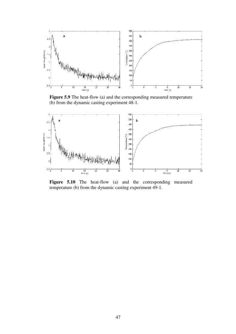
Figure 5.9 The heat-flow (a) and the corresponding measured temperature (b) from the dynamic casting experiment 48-1.
Figure 5.10 The heat-flow (a) and the corresponding measured temperature (b) from the dynamic casting experiment 49-1.
48
49
6 Conclusions
The presented method for calculating the heat-flow uses a finite difference algorithm for simulations of heat-flow, and is written in Matlab. It can be summarized as an automatic IHCP (inverse heat conduction problem) method. The IHCP algorithm is based on the principle to assume a heat-flow as a boundary condition for the heat conduction equation and compare the achieved numerical solution with results from the casting experiments. The created model is relatively simple and easy to understand. A commercial software, Abaqus/CAE, was used as reference. Abaqus/CAE could not achieve the desired heat-flow curves automatically, but was used as a control device for the created algorithm. Supposing that the experimental results were good, it was showed that the accuracy of the calculated heat-flow curves attained with the created algorithm were of good accuracy. The calculated maximal heat-flow into the steel substrate was 1.8 - 2.5 MW/m2 for the static casting experiments. For the copper substrate, the calculated maximal heat-flow was 2.8 MW/m2 for the dynamic tests and 4.32 - 6.45 MW/m2 for the static tests. A common problem for the casting experiments was the formation of a gap in the interface between the solidifying metal and the substrate. The cause of the gap could not be concluded from the experiments, but it is suspected that a high preheating temperature decreases the risk of gap formations. If this surface defect occurred in the region where the thermocouples were mounted, it led to distorted temperature measurements and thereby inaccurate heat-flow simulations. The casting simulator is helpful only in more advanced casting investigations if a smooth cast surface free from surface defects can be achieved. Another frequently occurring error, shown in Figure 2.9, was the shape of the achieved temperature curves. The deepest mounted thermocouple could sometimes show a higher temperature than the thermocouple closer to the surface. Peaks were also seen in the measured values and might be explained by bad thermal contact between the thermocouples and the substrate. These two effects might also be an effect of an uneven cast surface. When a gap occurs in the region of the mounted thermocouples or close to this region, the temperature gradient can no longer be assumed to exist in only one dimension. This is one of the fundamental assumptions made when creating the heat-flow model. If this condition fails, the corresponding calculated heat-flow curve also becomes incorrect. This can be an explanation to the unexpected low heat-flow in the dynamic cast experiment 47 and cu3 seen in Figures 5.4 and 5.8.
50
The noise levels in the temperature measurements were reduced by collecting data at a high sampling frequency and using as much over-sampling as possible. Increasing the distance between the noise generating sources (amplifier and stepper motor) and the DAQ/3000 device also decreased the noise. The noise could not be concluded to occur from some specified frequency.
51
7 Future work
The achieved heat-flow curve is calculated from one local temperature location in the substrate. By mounting a number of thermocouples in a grid pattern into the substrate, a more advanced heat-flow model could be obtained. Accurate and precise temperature measurements are of great importance for estimation and calculation of the interfacial heat-flow. Small errors in the temperature measurements can be amplified and cause large errors in the calculated heat-flow. Many casts had high error levels in the temperature data, caused by bad thermal contact, noise, and uneven cast surfaces among others. Therefore, more work has to be done to find efficient ways of granting good thermal contact and to reduce these error sources.
52
53
References
[1] A. Laveskog, (1976). Om metaller, Liber förlag, Stockholm. [2] J.R. Davis, (1994). ASM Speciality Handbook, Aluminum and Aluminum Alloys, ASM International, Cleveland. [3] J. Beddoes, M.J. Bibby, (1999). Principles of Metal Manufacturing Processes, John Wiley & Sons Inc., London [4] S.W. Barker, M. Gallerneault, B. Sutter, (2001). In: M. Sahoo, T.J. Lews (Eds.), Light Metals 2001, Toronto, Canada, pp. 133–144. [5] G. Evans, J. Blackledge, P. Yardley, (2000). Numerical methods for partial differential equations, Springer-Verlag London Limited. [6] G. Sparr, A. Sparr, (2000). Kontinuerliga system, Studentlitteratur, Lund. [7] A.D. Snider, (1999). Partial differential equations: Sources and solutions, Prentice Hall, Upper Saddle River, New Jersey. [8] R.D. Richtmyer, K.W. Morton, (1994). Difference methods for initial-value problems, Robert E. Krieger Publishing Co, New York.
54
55
Appendix A – Abaqus/CAE
Manual for Simulating Heat-flows in ABAQUS/CAE. ABAQUS/CAE is a complete environment that provides a simple, consistent interface for creating, submitting, monitoring, and evaluating results from the ABAQUS simulations. ABAQUS/CAE is divided into modules, where each module defines a logical aspect of the modeling process, for example, defining the geometry, defining material properties, and generating a mesh. As you move from module to module, you build the model from which ABAQUS/CAE generates an input file that you submit to the ABAQUS/Standard or ABAQUS/Explicit solver. The solver performs the analysis, sends information to ABAQUS/CAE to allow you to monitor the progress of the job, and generates an output database. Finally, you use the Visualization module of ABAQUS/CAE to read the output database and view the results of your analysis. ABAQUS/CAE has no built-in system for units. All input data must therefore be specified in consistent units. This instruction will use the SI (metric) unit system.
56
The module-list under the toolbar lists the modules in a logical sequence and you can move back and forth between modules at will. The following modules will be used in this heat-flow simulation: 1. Part Sketches a profile and creates a part representing the
substrate. 2. Property Defines the material properties of the substrate. 3. Assembly Assembles the model. 4. Step ConFigures the analysis procedure and output requests. 5. Load Applies a load (heat-flow) to the substrate. 6. Mesh Meshes the substrate. 7. Job Creates a job and submits it for analysis. 8. Visualization Views the results of the analysis.
Figure A1 The ABAQUS/CAE modules.
57
1. Part
How to create the substrate
• In the Module list located under the toolbar, click Part to enter the Part module. From the main menu bar, select Part Create to create a new part.
• The Create Part dialog box appears. ABAQUS/CAE also displays text in the prompt area near the bottom of the window to guide you through the procedure.
Name the part Substrate. Set the modeling space to 2D planar, the type to deformable body and a base feature to shell. In the Approximate size text field, type 0.02. Click Continue to exit the Create Part dialog box. ABAQUS/CAE automatically enters the Sketcher. The Sketcher toolbox appears in the left side of the main window, and the Sketcher grid appears in the view port.
entities and undo ) are available in the toolbar to help you examine your model. Experiment with each of these tools until you are comfortable with them.
Click the icon and zoom out until you see the edges of the blue grid To sketch the profile of the cantilever beam, you need to select the rectangle
drawing tool. ABAQUS/CAE often displays a short message in the prompt area to guide you through the procedure. This can be very helpful. In the view port, sketch the rectangle using the following steps: Click one corner of the rectangle at coordinates (0, 0). Move the cursor to the opposite corner (0.005, –0.01) so that the rectangle is five grid-squares long and ten grid-squares high, as shown in fig A2.
Click the icon in the prompt area and then click Done.
58
Figure A2 Sketch of the rectangle.
2. Property
Creating a material
• In the Module list located under the toolbar, select Property to enter the Property module.
• From the main menu bar, select Material Create to create a new material. The Edit Material dialog box appears. Name the material AISI-1015-Steel.
Figure A3 The Edit material dialog box.
59
• From the material editor's menu bar, select General Density. ABAQUS/CAE displays the Mass density data form. Type a value of 7870 for the mass density in the field, as shown in Figure A3
• Select Thermal Conductivity and type 51.9 in the Conductivity data form.
• Select Thermal Specific heat and type 486 in the Specific heat data form.
Click OK to exit the material editor. Defining a section
• From the main menu bar, select Section Create.
• The Create Section dialog box appears. Name the section and accept default settings. Click Continue.
The Edit Section dialog box appears. Make sure that the material selection is AISI-1015-Steel. Accept the default selections and click OK. Assigning the section to the substrate
• From the main menu bar, select Assign Section. ABAQUS/CAE displays prompts in the prompt area to guide you through the procedure. Click anywhere on the substrate to select the region to which the section will be applied. ABAQUS/CAE highlights the entire substrate.
• Click Done in the prompt area to accept the selected geometry. The Assign Section dialog box appears containing your created section. Click OK to assign the homogeneous, solid section to the substrate. The Assign Section dialog box closes.
3. Assemble
Assembling the model
• In the Module list located under the toolbar, click Assembly to enter the Assembly module
• From the main menu bar, select Instance Create.
60
The Create Instance dialog box appears. In the dialog box, select your part and click OK.
4. Step
Creating an analysis step
• In the Module list located under the toolbar, click Step to enter the Step module
• From the main menu bar, select Step Create to create a step. The Create Step dialog box appears with a list of all the general procedures and a default step name of Step-1.
• From the list of available general procedures in the Create Step dialog box, select Heat transfer and click Continue.
The Edit Step dialog box appears.
• Make sure it is a transient response and change time period to 30 in the Basic tab.
• In the Incrementation tab, set type to fixed, maximal number of increments to 301 and increment size to 0.1.
• Click OK.
Figure A4 The Edit Step dialog box.
61
Doing this will create a 30 second simulation with 300 time-steps, where the time-interval between every step is 0.1 second.
5. Load
Applying the heat-flow as a function of time
In the Module list located under the toolbar, click Load to enter the Load module.
• From the main menu bar, select Tools Amplitude Create. The Create Amplitude dialog box appears.
• Select Tabular in the Create Amplitude dialog box and click Continue. The Edit Amplitude dialog box appears.
There are a number of possibilities how to enter the varying amplitude of the heat-flow into the Edit amplitude dialog box. You can create a separate file in Microsoft Excel or notepad with a time vs. amplitude matrix and import that file to ABAQUS, or you can type in your preferred values directly in the Edit Amplitude dialog box. If you do not have a separate amplitude file, or if this is the first time you create an ABAQUS model, follow the instructions below and skip the part Import a data file. Add data directly into the Edit Amplitude dialog box
Add the following numbers in the Amplitude Data tab:
• Insert each number and press [Enter] to add a new row.
• Click OK in the Edit Amplitude dialog box.
62
Import a data file
• Right-click in the time/amplitude column and choose Read from
File.
• The Read Data from ASCII file dialog box appears. Click select and browse for the file. An ASCII file selection dialog box appears.
• Choose the file you want and click OK.
• Click OK in the Read Data from ASCII file. The time/frequency and amplitude data appear in the edit amplitude dialog box shown in Figure A5.
Figure A5 Edit Amplitude dialog box.
• Click OK in the Edit Amplitude dialog box.
63
Create the load
• From the main menu bar, select Load Create. The Create Load dialog box appears.
• Make sure the Category is Thermal, select Surface heat flux and click continue.
• Select the top side of the substrate and click the done button in the status bar. A red line indicates the surface you have chosen.
The Edit Load dialog box appears.
• Type 1e6 in the magnitude field and change the amplitude to Amp-1 in the Amplitude field.
Figure A6 The Edit Load dialog box.
• Click OK.
64
6. Mesh
Creating the mesh
• In the Module list located under the toolbar, click Mesh to enter the Mesh module.
• From the main menu bar, select Mesh Controls. The Mesh Controls dialog box appears. ABAQUS/CAE colors the regions of your model to indicate which technique it will use to mesh that region.
• Accept the default settings and click OK to assign the mesh controls.
• From the main menu bar, select Mesh Element Type. The Element Type dialog box appears.
• In the dialog box, set family to heat transfer and set element controls to convection/diffusion in the Quad tab.
Figure A7 The element type dialog box.
• Click OK.
• From the main menu bar, select Seed Instance to seed the part instance.
65
The prompt area displays the default element size that ABAQUS/CAE will use to seed the part instance. This default element size is based on the size of the part instance. In the prompt area, erase the default element size of 0.001, type a value of 0.00025 and press [Enter].
• From the main menu bar, select Mesh Instance to mesh the part instance.
• From the buttons in the prompt area, click Yes to confirm that you want to mesh the part instance.
ABAQUS/CAE meshes the part instance and displays the resulting mesh, as shown in Figure A8.
Figure A8 The meshed substrate.
66
7. Job
Creating a Job file
• In the Module list located under the toolbar, click Job to enter the Job module.
• From the main menu bar, select Job Create. The Create Job dialog box appears.
• Name the job and click Continue. The Edit Job dialog box appears.
• Click the General tab and select the four checkboxes in the Preprocessor printout box shown in Figure A9.
Figure A9 The Edit Job dialog box.
• Click OK.
• From the main menu bar, select Job Manager to start the Job Manager.
67
The Job Manager appears and displays a list of your jobs, the model associated with each job, the type of analysis, and the status of the job.
• From the buttons on the right edge of the Job Manager, click Submit to submit your job for analysis.
Wait until the status of the job changes to Completed. You are now ready to view the results of the analysis with the Visualization module.
• From the buttons on the right edge of the Job Manager, click Results.
ABAQUS/CAE loads the Visualization module, opens the output database created by the job, and displays a representation of the model.
8. Visualization
Visualize the result
• From the main menu bar, select Plot Undeformed Shape. The visualized substrate changes from a blue rectangle to a green grid as shown in Fig A10
Figure A10 Visualization of the substrate.
68
• From the main menu bar, select Tools XY Data Create.
• Select ODB Field output in the dialog box that appears and click Continue.
The Report Field Output dialog box appears.
• In the Variables tab, Change the position to Unique Nodal and select the checkbox NT11: nodal temperature.
• Click the Elements/Nodes tab.
• Select Nodes in the item field and use Pick from view port as the Selection Method.
• Click a node at 1 mm depth under the substrate surface. This depth is equivalent to any node at the fourth row of nodes under the surface. A small red circle will appear at the node you choose.
• Click Done in the prompt area.
• To save the temporary data click Save in the dialog box. To show a time vs. temperature plot click Plot.
If the heat-flows in the Load module are the same as in this instruction, the plot should look as in Figure A11.
69
Figure A11 Temp (ºC) vs. Time (s) plot for node 703.
• To enter the saved data, select Tools XY Data Manager from the main menu bar.
The XY Data Manager dialog box appears. Select your saved data from the list and click Edit. You can now copy this table into Microsoft Excel and compare it to your measured temperatures.
70
71
Appendix B – Matlab code % simulering under 30s med tidssteget 0.001s och % "mesh-size" 0.25 mm, filtrerad signal close all; clear all; %%%%%%%%%%%%%%%%%%%%%%%%%%%%%%%%%%%%%%%%%%%%%%%%% %%%%%%%% mesh-size(h), timestep for HFL(deltatimeq) & loaded file %%%%%%%%%%%% h=0.5; k=0.01; r=k/h^2; x=(0:h:10); deltatimeq=10; thermo=1/h; %för temp 1 mm under ytan eps=0.0001; %Temp-difference (test-simulated) load statfe1.txt temp(:,:)=statfe1(:,:); for i=6:1:length(temp)-4 tal=0; for j=-5:1:4 temporary=temp(i+j,2); tal=temporary+tal; end; temp(i,2)=tal/10; end; %%%%%%%%%%%%%%%%%%%%%%%%%%%%%%%%%%%%%%%%%%% %%%%%%%% thermal properties %%%%%%%%%%%%%%%%%%%%%%%%% %steel C=486; ka=51.9e-3; rho=7870e-9; alpha=ka/(C*rho); %copper % C=385; % ka=385e-3; % rho=8960e-9; % alpha=ka/(C*rho); %%%%%%%%%%%%%%%%%%%%%%%%%%%%%%%%%%%%%%%%%%% %%%%%%%%%%%%%%%%%%%%%%%%%%%%%%%%%%%%%%%%%%% r=alpha*k/h^2; u(1000,length(temp))=zeros; u1(length(x),length(temp))=zeros; u2(length(x),length(temp))=zeros;
one=one+1; end; one for pl=1:1:one Figure(1) hold on plot(u(pl,:)); end; plot(temp(:,2),'--r'); hold off; xlabel('time (s)') ylabel(''Temperature(C)') u(size(u1))=zeros; u=((u2(:,:)+u1(:,:))/2); Figure(2) %plots simulated temp at x=0, x=1mm and experimental temp hold on plot(temp(:,2),'--k'); plot(u(length(x),:),'--g') plot(u(length(x)-thermo,:),'--r') xlabel('time (s)') ylabel('Temperature(C)') hold off; Figure(3) %plots the heat-flow curve qL(length(qL1))=zeros; qL(:)=(qL1(:)+qL2(:))/2; Figure(3) plot(-qL) xlabel('time (s)') ylabel('Heat-flow (MW/m2)') Figure(4) %plots the number of iteration used for every time interval plot(poop) axis([0 300 0 30]); xlabel('Step number') ylabel('Nuber of iterations')