Massively Parallel Solution of the BiGlobal EigenvalueProblem Using Dense Linear Algebra
Daniel Rodríguez! and Vassilis Theo!lis†
Universidad Politécnica de Madrid, E-28040 Madrid, Spain
DOI: 10.2514/1.42714
Linear instability of complex !owsmay be analyzed by numerical solutions of partial-derivative-based eigenvalueproblems; the concepts are, respectively, referred to as BiGlobal or TriGlobal instability, depending on whether twoor three spatial directions are resolved simultaneously. Numerical solutions of the BiGlobal eigenvalue problems in!ows of engineering signi"cance, such as the laminar separation bubble in which global eigenmodes have beenidenti"ed, reveal that recovery of (two-dimensional) amplitude functions of globally stable but convectively unstable!ows (i.e., !ows which sustain spatially amplifying disturbances in a local instability analysis context) requiresresolutions well beyond the capabilities of serial, in-core solutions of the BiGlobal eigenvalue problems. The presentcontribution presents a methodology capable of overcoming this bottleneck via massive parallel solution of theproblem at hand; the approach discussed is especially useful when a large window of the eigenspectrum is sought.Two separated !ow applications, one in the boundary-layer on a !at plate and one in the wake of a stalled airfoil, arebrie!y discussed as demonstrators of the class of problems in which the present enabling technology permits thestudy of global instability in an accurate manner.
NomenclatureDx, Dy = @=@x, @=@ymemd = memory required for one "oating-point complex
numbermemproc = memory available for computations on each
processorNarrays = number of arrays to be storedNvar = number of variables and equationsNx, Ny = Chebyshev–Gauss–Lobatto collocation points in the
x and y directionsp = number of processorsRe = Reynolds numbert = timetAR;it = time required for one Arnoldi iterationtEIG = time required for the eigenvalues and eigenvectors
calculationtEVP = time required for the eigenvalue problems creationtLU = time required for the matrix shifting and
velocity componentsx, y, z = streamwise, wall-normal, and spanwise spatial
coordinates
I. Introduction
L INEAR instability analysis of "ows has been a growing dis-cipline during the last century [1,2]. This theory permits deter-
mination of the conditions under which a given "ow ampli!es smallperturbations, thus evolving into a different (nonlinear) state; one ofthe key aims of linear theory is the prediction of laminar-turbulencetransition via solution of conceptually simple eigenvalue problems
(EVPs). In practice, the solution of the linear EVP resulting fromsuperposing three-dimensional small-amplitude perturbations upona three-dimensional basic "ow (i.e., "ow which is inhomogeneousin all three spatial dimensions) presents a numerically dauntingtask. Simpli!cations on the form of the basic "ow, the stability ofwhich is analyzed, are called for, the strongest of which is that of a“parallel” basic "ow, i.e., a steady one- or two-component, one-dimensional velocity pro!le. The numerical solution of thecorresponding EVP, of the Orr–Sommerfeld class, is currentlystraightforward and may be obtained with almost no restrictions.However, considering inhomogeneous basic "ows in two or threespatial directions results in partial-derivative EVPs, on occasionrequiring state-of-the-art algorithms and hardware for their solution.The present contribution discusses one such methodology for thesolution of the linear BiGlobal EVP.
Concretely, in incompressible "ow, the problem to be solved isobtained by assuming modal perturbations and homogeneity in onespatial direction, say the spanwise direction z. Eigenmodes areintroduced into the linearized Navier–Stokes and continuity equa-tions according to
!q"; p"# $ !q!x; y#; p!x; y##e%i!!z&!t# (1)
where q" $ !u"; v"; w"#T and p" are, respectively, the vector ofamplitude functions of linear velocity and pressure perturbations,superimposed upon steady two-dimensional, two- ( !w ' 0) or three-component, !q$ ! !u; !v; !w#T , steady basic states. The spanwise wavenumber ! is associated with the spanwise periodicity length Lz
through Lz $ 2"=!. Substitution of Eq. (1) into the linearizedequations of motion results in the complex BiGlobal eigenvalueproblem [3]
In the compressible case, an Ansatz analogous to Eq. (1) may besubstituted into the compressible linearized equations of motion.Although the form of the BiGlobal EVP is more involved [4,5], inthis case too, a system of (!ve) coupled equations for the disturbanceamplitude functions is obtained.
The spatial discretization of either compressible or incompressibleBiGlobal EVPs results in large matrices which, when stored in core,con!ne the resolution employed to low Reynolds numbers. On theother hand, "ows of industrial interest usually involve complexgeometries at high Reynolds numbers, requiring resolutions whichcannot be handled by the currently available top-end serial machines.
In this paper, two problems representative of the computationaldif!culties associated with the BiGlobal approach in open systemsare considered. The !rst problem is the instability of a laminarboundary layer on a "at plate with an embedded separation bubble.Unlike earlier works [6], where homogeneous Dirichlet boundaryconditions have been used to close the system and to permit theentrance of wavelike disturbances of the Tollmien–Schlichting classinto the integration domain, a Robin boundary condition is used atthe in"ow boundary. This boundary condition imposes a relationbetween thewave number and the frequency using information fromlocal analysis. Numerically, this boundary condition prohibitsreducing the EVP to one with real coef!cients. In addition, the com-putational domain must include several periods of the most unstable/least stable wavelike eigenmodes in the streamwise direction toadequately recover the physics. Furthermore, the spatial resolutionmust be adequate to recover the !ne structure of the instability wave,especially in the surroundings of the separation bubble. Finally, here,three-dimensional disturbances are recovered by solution of a systemof four coupled partial differential equations; this is in contrast toanalogous earlier studies [7,8] which solved a system of threecoupled partial differential equations (PDEs), thereby focusing ontwo-dimensional Tollmien–Schlichting waves alone. The secondproblem considered is the instability of the "ow around a stalledNACA0015 airfoil. This problem is physically related to the previousone, but is more interesting from an industrial point of view. Acoordinate transformation implemented for its solution [9] torepresent this relatively complex geometry introduces new nonzeroterms in the matrix discretizing the EVP, as will be discussed later. Inthis application too, a large domain is necessary to reduce the in"u-ence of the nonphysical boundary conditions imposed at the far-!eldboundary and, together with the nonlocalized structures appearing inthe eigenmodes, extremely large resolutions are required.
Typically, these problems are addressed by using a time-steppingmethod for the numerical solution of the BiGlobal EVP [10–12].Time-stepping approaches were devised at a time when storage oflargematriceswas impractical andwork optimally for the recovery ofa small number of leading eigenmodes. If additional modes arenecessary (as, for example, in the case of transient growth analysis), anew time-stepping iteration, which excludes the modes alreadyidenti!ed, is necessary.
Here, an alternative methodology is presented, which forms thediscretized matrix and stores it over several processors of a com-puting cluster; using distributed-memory parallel computers, themaximum dimension of the problem which may be solved is thusdetermined by the number of processors available. The combinationof distributedmatrix formation and storage in conjunctionwith denselinear-algebra software is employed to the problem at hand for the!rst time.
The proposed solution relaxes both the memory restrictionsassociated with the matrix formation and the CPU time limitationsimposed by a serial solution of the EVP. Linear-algebra operationsare performed by the ScaLAPACK, BLACS, and PBLAS parallel,dense linear-algebra libraries [13]. These libraries are outgrowths ofthe well-known, well-tested LAPACK project and have beendocumented to work in a satisfactory manner with dense matrices ofleading dimension O!106# achieving (100 tera"ops on (20; 000
processors [14]. Supercomputers with several thousand processorsfeaturing the proposed linear-algebra libraries, such as Magerit‡ orMare Nostrum,§ are becoming widely available and are increasinglydeployed for the solution of large-scale scienti!c problems [15].
The paper is organized as follows: in Sec. II, the proposedmethodology is presented, including information on the spatialdiscretization and the matrix distribution. Section III presents resultsobtained, both from a numerical and a physical point of view.Validation and veri!cation work is presented in Sec. III.A, where thecapabilities of parallelization are demonstrated. Themain body of thescalability studies is presented in Sec. III.B, exclusively devoted tomassive parallelization of the eigenvalue problem. The two physicalinstability problems which gave rise to devising of the presentsolution methodology are presented in Sec. III.C; in both problemsmonitored, the large resolutions employed have been instrumentalfor the success of the analysis. Conclusions and some discussion ofalternatives to the methodology presented are discussed in Sec. IV.
II. Massively Parallel Eigenvalue ProblemSolution Methodology
BiGlobal EVPs involve square matrices of large leading dimen-sion resulting from the spatial discretization of four (!ve for thecompressible case) coupled partial differential equations. Numericalsolution of such problems is facilitated by numerical methods of aformal accuracy as high as possible, capable of minimizing thenumber of discretization nodes and thus keeping the memory re-quirements as low as possible. Spectral methods have such charac-teristics, although they come at the price of dense matrices, whichmake implementation of sparse solution techniques not straightfor-ward. On the other hand, the coupled discretization of two spatialdimensions results in matrices with a certain degree of sparsity, evenwhen using spectral methods. Here, only the treatment of theBiGlobal EVP problem using dense linear-algebra operations isconsidered. Experience with spectral methods for the solution of theBiGlobal EVP suggests that this numerical discretization method-ology requires matrices of leading dimension O!104 ( 105# for thecoupled discretization of the two spatial directions. On the otherhand, experiencewith both spectral and !nite difference methods forone-dimensional (ordinary-differential-equation-based) stabilityproblems [16,17] has delivered a rule of thumb for the number ofnodes required by a spectral and a !nite difference numerical methodto obtain results of the same accuracy. This rule of thumb depends onthe order of the !nite difference discretization; use of a sixth-ordercompact !nite difference scheme requires a factor four highernumber of nodes compared with a spectral method of equivalentaccuracy [18]. Extrapolation of such results to the (two-dimensional,partial-differential-equation-based) BiGlobal EVP suggests that ahigh-order !nite difference approach would require discretizedarrays the leading dimension of which would be at least 1 order ofmagnitude higher than that quoted previously; such arrays wouldonly be able to be treated by sparse-matrix techniques. By contrast,spectral methods and dense-matrix algebra has been used presently,as follows.
A. Spatial Discretization
Spatial discretization is accomplished by Chebyshev–Gauss–Lobatto (CGL) points
#$ cosi"
N; i$ 0; . . . ; N (7)
and the correspondent derivative matrices D$ @=@#, D!2# $D )D; . . . ;D!n# [19]. The CGL points are mapped onto the domain ofinterest by coordinate transformations, which permit clustering ofnodes in speci!c regions of the domain, like in boundary layers.Tensor products are used to form the derivative matrices for thepresent PDE-based problem. If Nx % 1 and Ny % 1 collocation
‡Data available at www.cesvima.upm.es.§Data available at www.bsc.es.
2450 RODRÍGUEZ AND THEOFILIS
points are used for the discretization of the x- and y-spatial directions,respectively, the discrete resulting differentiation matrices have aleading dimension of !Nx % 1# * !Ny % 1# and are obtained byapplying the Kronecker product
D x $D+ I; Dy $ I +D (8)
where I is the identity matrix. Applying this spectral discretization tothe linear problem in Eqs. (2–5) results in a nearly block-diagonaldiscretizedmatrix problem, shown in Fig. 1,withmatrices of (global)leading dimension GLD$ Nvar * !Nx % 1# * !Ny % 1#, the factorNvar being equal to four in the incompressible case, arising from thefour coupled equations, and !ve in the compressible case. The
structure of the matrices, in which many elements are equal to zero,makes it possible to implement sparse techniques to drasticallyreduce the memory requirements. This possibility was tested in aprevious research [20] using the parallel version of the librarySuperLU, but the scalability was shown to be unsatisfactory. Suchsparse techniques are not used here; instead, the problem is treated asone of dense matrices, which permits greater "exibility in intro-ducing variations to the linear operators (i.e., different types ofboundary conditions) without altering the data storing and solutionalgorithms. The linear operators describing the physics and thenumerics and parallelization used to solve the problem are indepen-dent. In this manner, it is possible to solve both compressible andincompressible problems with an arbitrary combination of boundaryconditions by making only minor changes in the core solutionalgorithm. The structure of the left-hand-side (LHS) matrices corres-ponding to both incompressible and compressible problems areshown in Fig. 1.
B. Arnoldi Algorithm
The large leading dimension of the complex matrices resultingfrom the discretization of the problem Eqs. (2–5) makes the appli-cation of the QZ algorithm (generalized Schur decomposition) [21]impossible. In contrast, Krylov subspace-based algorithms are usedto recover ef!ciently the most interesting part of the eigenspectrum.A shift-and-invert variation of the Arnoldi algorithm [22] is em-ployed here to transform the large EVP into a several orders-of-magnitude smaller problem (having a leading dimension equal to theKrylov subspace dimension, m( 200–2000). The QZ algorithm isused then to obtain the solution of the latter problem.
AnArnoldi algorithm is used; its twomain tasks are a lower–upper(LU) decomposition of the large left-hand-side matrix in Eqs. (2–5)and a certain number of back substitutions equal to the dimension oftheKrylov subspace generated. The!rst task accounts formost of theCPU time required in the serial solution, the latter methodologyhaving been employed in the past in a satisfactory manner. However,resolution of physical phenomena involving steep gradients and/orseveral structures (e.g., Tollmien–Schlichting waves as amplitudefunctions of a BiGlobal eigenvector) give rise to the need for a step-change improvement. Such a borderline case has been encounteredin the problem of instability of the laminar separation bubble atmoderate Reynolds number [23]; using a number of discretizingpoints ofNx $ Ny $ 60 translates into a LHS matrix leading dimen-sion O!15; 000#, requiring O!3:5# GB of in-core memory, andtaking nearly 2 h of CPU time in a fast, shared-memory computer.
C. Data DistributionUsing ScaLAPACK, the parallelization is understood as a two-
step approach. First, a virtual, rectangular processor grid is formedusing all the processors available. Second, the arrays that store bothmatrices and vectors are distributed amongst the processor’s gridfollowing the block-cyclic algorithm [13]. In this second step, eacharray is divided into blocks, that is, small pieces of the arrays with anumber of rows and columns given by an user-de!ned parametercalled blocking factor (BF). ScaLAPACK permits using a differentblocking factor for rows and columns, but according to the squarematrices to be operated on, an unique value of BF was used for both.The distribution algorithm works independently on rows andcolumns. To illustrate the distribution, suppose an array of lengthGLD (with entries numbered from 1 to GLD) to be stored on pprocessors (numbered 0 through p & 1). The array is divided intoblocks of size BF, except the last block which will contain GLDmodBF elements in the most general case. These blocks are numberedstarting from zero and are distributed amongst the processors, so thatthe kth block is assigned to the processor of coordinate kmod p. Thealgorithm results in that the element IG (which is the index of theelement on the global matrix) from the original global array maps tothe element IL (which is the index of the element on the local matrix)of the local matrix assigned to the processor IP (which is the index ofthe processor on the processor’s grid), where IL and IP are de!ned by
Fig. 1 Block-diagonal structure of the incompressible BiGlobal EVPleft-hand side matrix in Eqs. (2–5) (top) and the equivalent compressibleproblem (bottom), when discretized using spectral collocation methods.For these matrices, Nx ! Ny ! 10 Chebyshev–Gauss–Lobatto pointswere used.
RODRÍGUEZ AND THEOFILIS 2451
IL $ BF *!IG & 1
BF * p
"% !IG & 1modBF# % 1 (9)
and
IP $!IG & 1
BF
"modp (10)
More details on the distribution algorithm can be found inScaLAPACK’s documentation [13]. The arrays are stored in abalanced manner using the memory of all the processors available.The difference in the number of elements contained in the local arraysis, at most, equal to the blocking factor, which should be chosen to beorders-of-magnitude smaller than the global leading dimensions, aswill be shown later. The main memory constraint in the solution ofthe BiGlobal EVP is the storage of one large matrix for the incom-pressible case (two for the compressible case), of leading dimensionGLD. Other arrays also need to be stored, both in distributed ornondistributed manners, but its size is negligible compared to thelarge matrices. The minimum number of processors required for thesolution of the problem is then estimated as
p, Narrays * GLD2 * memd
memproc
(11)
where Narrays is the number matrices to store, memd is the memoryrequired for the storage in "oating-point format of one complexmatrix element (i.e., 16 B using double precision), andmemproc is thememory available for the computations per processor. Because of thealmost diagonal structure of the right-hand-side matrix in the incom-pressible problem, only the storage of the left-hand-side matrix isrequired and Narrays $ 1. Conversely, in the compressible case, theright-hand-sidematrix ismore involved, and the twomatrices need tobe stored (Narrays $ 2). A small amount of memory is required forthe other variables, the relative amount becoming smaller withincreasing GLD. In any case, as will be discussed later, betterperformances are attained when a higher number of processors thanthe minimum is used.
III. ResultsA. Veri"cation and Validation
The problem of stability in a constant pressure-gradient drivenrectangular duct [24,25] has been solved as a validation test. Thisproblem has been chosen on the basis of two characteristics:
1) The required basic "ow is recovered as the solution of therelated Poisson problem
r22D !w$&2 (12)
subject to homogeneous Dirichlet boundary conditions. The ana-lytical solution of the problem is known and can be used both tocheck the convergence of the discretization and the performance ofthe parallel LU decomposition.
2) There is no transformation which permits converting thecomplex BiGlobal EVP into an equivalent EVP with realcoef!cients.
The physical instability in the rectangular duct "ow is encounteredas a consequence of increasing the aspect ratio ! or increasing theReynolds number at low !nite values of! " 1¶; in either case, theresolution requirements increase beyond the maximum memoryavailable on a typical serial machine. A case in which high resolutionis required, and as such could be used to implement the distributed-memory techniques discussed herein, is the critical point of an aspectratio !$ 5 duct, Re$ 10; 400, !$ 0:91 [25]. The convergencehistory is shown in Table 1.
In terms of the theme of the present paper, when the number ofcollocation points is less than 40 * 40, it is impossible to determinethe value of the critical eigenvalue, due to the proximity of manyunresolved eigenvalues. The convergence of the third decimal place
in!r is attained for a resolution of 70 * 70; this translates in 6 GB ofin-core memory, more than that available on most serial computers.The convergence of the sixth decimal place is attained at a resolutionof 110 * 110 nodes per amplitude function. This requires in excess of36 GB and is clearly impossible to be handled by a typical serialmachine.
B. Scalability and Massive Parallelization
Themain objective of this work is to break the barrier in resolutionimposed by the limited memory available on even the most power-ful shared-memory machines. Distributed-memory parallelizationmakes it possible to store and compute with matrices whose size isonly a function of the number of processors available, whiledrastically reducing the CPU time required for calculations. Threecomputing clusters have been used for the present work; theircharacteristics are summarized in Table 2. Aeolos is an own-localdistributed-memory machine formed by 128Myrinet interconnectedxeon microprocessors, with own-compiled versions of BLACS andScaLAPACK. At the other end, Mare Nostrum has been used; thismachine is currently the number 13, top 500 supercomputer (at thetime testing commenced, was at number 5), and is situated at theBarcelona Supercomputing Center and comprises 10240 IBM970MP processors, interconnected by Myrinet and Gigabit Ethernetnetworks. Mare Nostrun features the IBM optimized version ofScaLAPACK, PESSL. Between the two cluster extremes, anotherlocal facility, Magerit, has been used. Magerit comprises 1200eServer BladeJS20, each one with two power-PC microprocessors,interconnected by the Myrinet network, and also features PESSL, amachine-optimized version of ScaLAPACK.
A!rst scalability test was performed using the solution of Eq. (12),as it involves only the construction of a distributed matrix and theparallel LU decomposition. The local cluster Aeolos was used forthese computations comprising different values of the blockingfactor and matrix leading dimension. Two results are of signi!cancehere, one that the suggested [13] value of the blocking factor BF$64 for both directions corresponds to the lowest wall time at allprocessor-grid con!gurations examined; as such, in subsequentcomputations, this parameter has been kept at its !xed optimal value.Secondly, and probablymost signi!cant, a near-perfect linear scalingis observed when the number of processors is increased, at allblocking-factor values. The latter result has been con!rmed withsolutions of both smaller and larger leading dimension matrices. Theresults of this !rst test are summarized in Fig. 2. The parallel solutionusing 16 processors reduces the computing time to less than an hourand the use of 64 processors reduces the time required for the serialsolution by a factor of 36.
A second scalability test used Aeolos and Mare Nostrum, bysolving the BiGlobal EVP of the instability of rectangular duct "owat Re$ 100 and !$ 1. The results obtained using different resolu-tions and number of processors are shown in the left part of Fig. 3.When the low (though perfectly adequate for convergence of theeigenmode) resolution 40 * 40 is used, the wall-time reduction withthe number of processors is not signi!cant, staying in the same orderof magnitude of the serial solution. As resolution is increased, thetheoretically constant CPU-time/number of processors ratio
Table 1 Convergence history for the critical eigenvalue correspondingto the rectangular duct with!! 5 at Re! 10; 400 and !! 0:91;
reference frequency result!r ! 0:21167 [24,25] (leading dimension andrequired memory corresponding to the stored matrix are also shown)
¶Flow is linearly stable in a square-duct con!guration [24].
2452 RODRÍGUEZ AND THEOFILIS
Tp $tCPUp
(13)
is visible in the results: the time required to solve a 60 * 60 domainon four processors is almost 25 min; it is reduced to 12 min for eightprocessors and to 7 min on 16 processors. As mentioned earlier,solution of this problemwas found to require almost 2 hCPU time ona serial machine. The same validation test was also solved on MareNostrum, using a number of processors from 64 to 1024. The resultsare shown in the right part of Fig. 3. The large, maximum number ofprocessors used, 1024, makes it possible to increase resolution up to256 * 256. The CPU time required when the 80 * 80 domain issolved always stays under 10 min, but scales poorly with the numberof processors; wall-clock time is even found to increase when morethan 512 processors are employed.When the resolution is increased,in this case to 128 * 128, the constant Tp scaling is recovered.
Conclusions drawn from this part of the work are as follows. Asmentioned in the ScaLAPACKdocumentation, aworkload balance isrequired for the code to scale satisfactorily, that is, so that thetheoretically constant Tp is attained. If the local matrix, that is, thesubmatrix stored in each processor is too small, most of thewall timeis spent on communication between processors; in that situation, thematrix is said to be overdistributed. On the other hand, if the localmatrix is too large, most of the calculations take place inside eachcomputer and better performance can be achieved by using a largernumber of processors. A rule of thumb states that the dimension ofthe local matrices should be of size(1000 * 1000. The existence ofan optimal number of processors to solve a given problem is evident,and this optimal value should be studied for each resolution. Typicalacademic BiGlobal EVPs require resolutions corresponding to anumber of processors below 512; however, as this theory enters therealm of industrial applications, for which the Reynolds numbersinvolved are orders-of-magnitude higher than those of academicproblems, resolutions comprising hundreds of points for eachdirection are required. A last conclusion concerns thewall-clock timeversus number of processors, assuming a correct workload balance.The ideal constant value for the Tp is nearly accomplished when the
LU factorization occupies around half of total wall-clock time, thematrix generation costs about 20% of the total time, and all othertasks together account for the last 30%. However, when the numberof processors is increased, effects other than the main parallel task,the LU decomposition, become increasingly more relevant.
It is therefore appropriate to turnattention toquantifying scalabilityunder these conditions next, focusing on problems for which thedimensions are more representative of the current requirements ofBiGlobal EVPs. Inwhat follows, four aspects are studied: Sec. III.B.1monitors the time required for the (manual) creation of the left-hand-side matrix in a distributed manner; Sec. III.B.2 deals with the LUdecomposition of the EVP matrix, using ScaLAPACK; Sec. III.B.3studies (in an average manner) the time devoted to the Arnoldiiteration, and Sec. III.B.4 is dedicated to the QZ subroutine of theHessenberg matrix and the calculation of the eigenvectors.
1. Eigenvalue Problem Generation
In the previous section, the creation, in a distributedmanner, of thelarge leading-dimension matrices describing the eigenvalue pro-blem (2–5) was found to consume a considerable amount of time((20% of the total). This is in contrast to the serial solution of thesameproblem,where this fraction of time is negligible. The origins ofthis result are to be found in the fact that the dimension of thematricesgrows with the square of the resolution used. Concretely, the fol-lowing operations are needed to generate thematrices: 1) double loopover the global matrix dimension: t( !GLD#2; 2) value assign-ment to the correspondent element and processor: t( !GLD#2=p;3) certain number of loops over the matrix dimension: t( GLD.
When the leading dimension of the globalmatrix GLD is large, thetime required for the EVP generation scales as
tEVP (!1% K
p
") !GLD#2 (14)
K being a constant that depends on the processor and communi-cations speeds. Studies were conducted to evaluate how well thistheoretical scaling is attained. The test problem was solved using aconstant number of collocation points in the y direction (Ny $ 40), avariable number of points in the x direction, and a different number ofprocessors. The CPU time required for the creation of the globalmatrix was computed and the results are shown in the left part ofFig. 4. Thicker, dashed lines belong to Aeolos, whereas solid linesbelong to Magerit. With minor deviations, the behavior of the CPUtime is that described by Eq. (14). To isolate the !rst-order behavior,the same time is scaled with GLD and p,
tEVP ) pGLD2
( !p% K# % K2 ) pGLD
(15)
taking into account second-order effects, whose relative contributionis unknown a priori. This new variable is plotted againstNx and p inthe right part of Fig. 4. The coincidence of the scaled data in the lower!gure indicates that the constant K2 is small enough to neglect itseffect. This constant is related to the third operation stated before.The time consumed for a given resolution and number of processorsis higher in Magerit that in Aeolos. As no library subroutine is usedand there is no communication between processors in this task, thisdifference is attributed to a higher speed of the processors of Aeolos.
2. Lower–Upper Decomposition of the Global Matrix
The LU decomposition is the most time-consuming task in boththe serial and parallel versions of the code; serially, it accounts forover (90% of the total CPU time, whereas this percentage drops to
Fig. 2 Wall time for the parallel solution of the Poisson model problemas a function of the number of processors and the blocking factors used.
Table 2 Characteristics of the distributed-memory machines used
Cluster No. processors Processors Network Library
Aeolos 128 Intel Xeon Myrinet Own-compiled ScaLAPACKMagerit 2400 IBM PPC Myrinet and Gigabit PESSLMare Nostrum 10,240 IBM 970 MP Myrinet and Gigabit PESSL
RODRÍGUEZ AND THEOFILIS 2453
(50% in a typical parallel solution. Although ef!ciency of the codein this task depends entirely on the library software, !ne tuning thediscretization parameters in the parallel version of the code isessential to obtain optimal performances. The time required forshifting the matrix is also computed in this section but, as will beshown, this time is negligible compared to the time devoted to the LUdecomposition. The operations required in this context are 1) loopover the matrix dimension: t( GLD; 2) value assignment to thecorrespondent element and processor: t( GLD=p; 3) LU decom-position, by call to the subroutine: t( !GLD#3=p.
When the leading dimension of the matrix is large, the theoreticalprediction for the scaling is
tLU ( !GLD#3p
(16)
The same scalability tests as in the previous section wereconducted, and results are shown in the left part of Fig. 5. The trendspredicted from the !rst-order scaling Eq. (16) are reproduced in all
cases. To recover second-order effects, the CPU time is scaled withGLD and p:
tLU ) pGLD3
( K % K2 ) p% K3
GLD2(17)
where K, K2, and K3 are constants different to the ones de!nedearlier, but related to the same issues. The scaled times are plottedagainst GLDandp on the right side of Fig. 5. The relative importanceof the LU decomposition is even increased over the shifting timewhen the dimension of thematrix grows, as the scaled time is reducedwith increasing resolutions. The bene!ts of using the optimizedlibrary and massive parallelization are evident from the !gures,because the scaled time decreases substantially from Aeolos data toMagerit, the latter platform affording substantially higher resolu-tions due to the larger number of processors available. Theimportance of the correct data parallelization may be observed onthe lower-right plot. The documentation of ScaLAPACK suggeststhat the processor grid be as square as possible for performance to
Fig. 4 CPU time scaling for EVPgeneration. The time (left) and time scaledwith the number of processors andLHSmatrix size (right) is plotted againstthe resolution (top) and number of processors (bottom). Thicker, dashed lines belong to Aeolos; solid lines belong to Magerit.
Fig. 3 Scalability tests performed on Aeolos (left) and Mare Nostrum (right). The CPU time required for the solution of the eigenvalue problem (LUfactorization and Arnoldi algorithm) is plotted against the number of processors (procs) for various resolutions (in parenthesis). In brackets, the leadingdimension of the LHS matrix is shown.
2454 RODRÍGUEZ AND THEOFILIS
be optimized. The processors’ grids de!ned in this !gure are asfollows: 4 * 4 !p$ 16#, 5 * 5 !p$ 25#, 4 * 8 !p$ 32#, 6 * 8!p$ 48#, 8 * 8 !p$ 64#, and 8 * 16 !p$ 128#. In the resultsshown in the lower-right part of Fig. 5, it can be seen thatperformance at the square processor grid 8 * 8 is much better thanthat on any other processor distribution.
3. Arnoldi Iteration
TheArnoldi algorithm generates aKrylov subspacewhose dimen-sion m is orders-of-magnitude smaller than GLD. Nevertheless, mmust increase as the resolution increases, in line with the increase ofthe number of processors used. The time required for each Kryloviteration is generally small but, if the Krylov subspace dimension ishigh, the cumulative time cannot be neglected. Here, the timerequired for each iteration is averaged over m$ 200 iterations. The
different calculations performed within each Krylov iteration requiretime consumption in several places, of which only the more relevantare taken into account next: 1) loop over the globalmatrix dimension:t( GLD; 2) value assignment to the correspondent element andprocessor: t( GLD=p; 3) backsubstitution on the LU decomposedmatrix: t( !GLD#2=p.
When the leading dimension of the matrices is large, the leading-order effect on time is
tAr;it (GLD2
p(18)
The results of the scalability tests are shown in the left part ofFig. 6. The time consumed increases with increasing resolution,but almost linearly rather than the expected quadratic trend. The
Fig. 5 CPU time scaling for shift and invert and LU decomposition. The time (left) and time scaled with the number of processors and LHSmatrix size(right) is plotted against the resolution (top) and number of processors (bottom). Thicker, dashed lines belong to Aeolos; solid lines belong to Magerit.
Fig. 6 CPU time scaling for one Arnoldi iteration. The time (left) and time scaled with the LHSmatrix size (right) is plotted against the resolution (top)and number of processors (bottom). Thicker, dashed lines belong to Aeolos; solid lines belong to Magerit.
RODRÍGUEZ AND THEOFILIS 2455
variation with the number of processors also shows the predictedtrend, but has an important deviation for a given (i.e., p$ 48)processor grid. The conclusion drawn is that what was assumed to besecond-order effects are more signi!cant than implied by the scalingEq. (18). The alternative time scaling is then constructed:
tAr;itGLD2
( K
p%!K2 %
K3
p
") 1
GLD(19)
Here, the time required for tasks 1 and 2, supposed negligible inEq. (18), has amore pronounced effect and increases the ef!ciency asthe resolution becomes higher, as can be seen in upper-right part ofFig. 6. The lower-right part of the same !gure shows that, althoughthe scaled time versus number of processors is correctly described byEq. (18), the relation to the shape of the processor’s grid is not fullyunderstood. The most plausible explanation relates the increase intime to one ormore tasks, severely affectedwhen the processor’s gridis not square. The ScaLAPACK suggestion about the shape of theprocessor’s grid has been taken into account here, but the exactcause in the performance degradation in the backsubstitution task isunclear. The fact that better performance is obtained in Mageritsuggests use of the optimized library version as a possibleexplanation.
4. Eigenvalues and Eigenvectors Calculation
Once the Krylov subspace and Hessenberg matrix have beengenerated, most of the tasks are performed in each processor in aserial manner, with no communication between processors. Eachprocessor stores a copy of the Hessenberg matrix and calls the QZsubroutine independently; although this approach generates largeredundancy, it is faster than computing the eigenvalues in oneprocessor only and communicating the data between a large numberof processors. On the other hand, once the eigenvectors from theHessenberg are computed, they must be distributed to compute theRitz vectors by forming their product with the Krylov subspace base.This combination of serial (Hessenberg matrix eigensystem com-putation) and parallel (matrix–matrix product) tasksmakes it dif!cultto estimate scalings, but much of the workload is distributing dataover the processors, and so it is expected that increasing the numberof processors will increase the CPU time. Themajor time-consumingtasks are as follows: 1) double loop over the Hessenberg matrixdimension in each processor: t( !m#2 ) p; 2) product of distributedmatrices: t( !m#2 ) GLD=p; 3) loop over the global matrixdimension in each processor: t( GLD ) p.
Little can be said about the relative importance of each contri-bution at this point. As the resolution and Krylov subspace dimen-sion should grow together for approximately the same fraction of theeigenspectrum to be computed, an increment in resolution will resultin an increment of CPU time. On the other hand, and contrary towhathappens in other tasks, the required time grows linearly with thenumber of processors if p is high enough. This theoretical behaviorhas been recovered in the numerical experimentation performed, as isshown in the left part of Fig. 7. Time was scaled with the globalmatrix leading dimension, as the dimension of theHessenbergmatrixwas kept constant in all tests:
tEIGGLD
( K % p )!K2 %
K3
GLD
"(20)
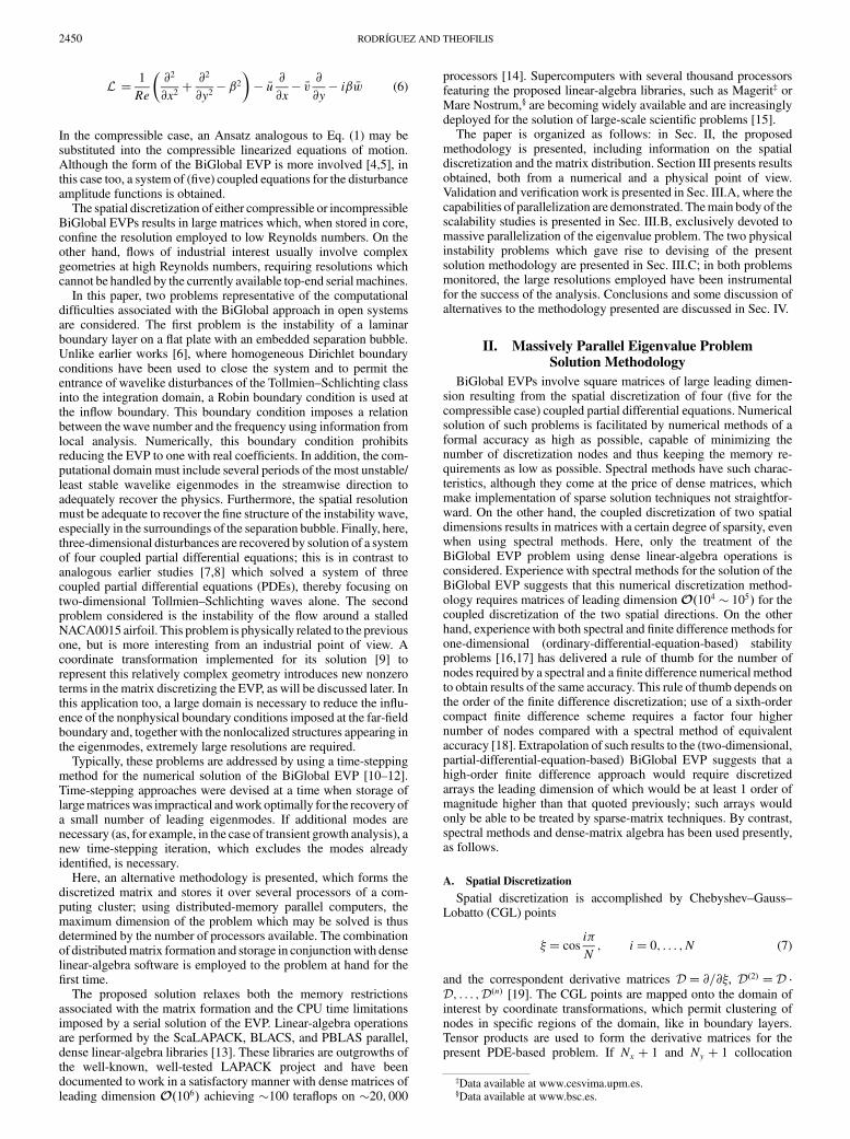
The dependence of this scaled timewith the resolution and numberof processors is plotted in the right part of Fig. 7. There is no variationof the scaled time with the resolution, and so the term multiplied byK3 is neglected. The number of processors has an important effect onthe ef!ciency of the code, as an increase inp drastically increases thetime tEIG. In this respect Aeolos was found to be much more ef!cientthan Magerit in performing this task, the time being almost inde-pendent of the number of processors, probably due to better internalcommunications between the processors in the former, as opposed tothe latter platform. A summary of our !ndings on the relative timerequired for each one of the main parallelization tasks is shown inFig. 8. When the number of processors is !xed, the relative impor-tance of the LU-decomposition time increases with the resolution,reducing the corresponding contribution ofArnoldi iterations and theeigenvalues and eigenvectors computation. When the resolution is!xed, the time required for the computation of eigenvalues andeigenvectors grows notably, being the factor which imposes anoptimal number of processors. The time required for the EVPgeneration is around one-!fth of the total CPU time.
C. Applications to Separated Flow Instability
The present methodology enables use of high resolutions aspermitted by the number of processors available; the nearly linearscaling demonstrated implies that the CPU time necessary for therecovery of a given window of eigenvalues is an inverse linearfunction of the number of processors used. This approach haspermitted the study of problems out of reach of previously availablemethodologies of the same class. Two examples are shortly exposed,one representative of open problems in which the convective nature
Fig. 7 CPU time scaling for eigenvalues computation. The time (left) and time scaled with the LHS matrix size (right) is plotted against the resolution(top) and number of processors (bottom). Thicker, dashed lines belong to Aeolos; solid lines belong to Magerit.
2456 RODRÍGUEZ AND THEOFILIS
of the dominant instability dictates use of large resolutions, and asecond application, closer to industrial interests, inwhich, in additionto the previous considerations, a relatively complex geometry has tobe dealt with.
1. Instability of Laminar Separation Bubble in a Flat-PlateBoundary Layer
This application has been discussed in detail elsewhere [26]. Thebasic "ow corresponds to a "at-plate boundary layer with Reynoldsnumber based on the displacement thickness at the in"ow equal to450 at in"ow and 700 at out"ow, and a separation bubble with peakreversed "ow (1% of the far-!eld velocity. This two-dimensional"ow is analyzed with respect to its three-dimensional global insta-bility within the entire range of spanwise wave numbers ! 2 -0;1#;in practice, a large number of eigenvalue problems, each corres-ponding to a given discrete value of !, are analyzed. The entrance ofTollmien–Schlichting waves through the in"ow is permitted byimposing the Robin boundary condition
@q@x
$.i$q; where $, $0 % c0!! & !0# (21)
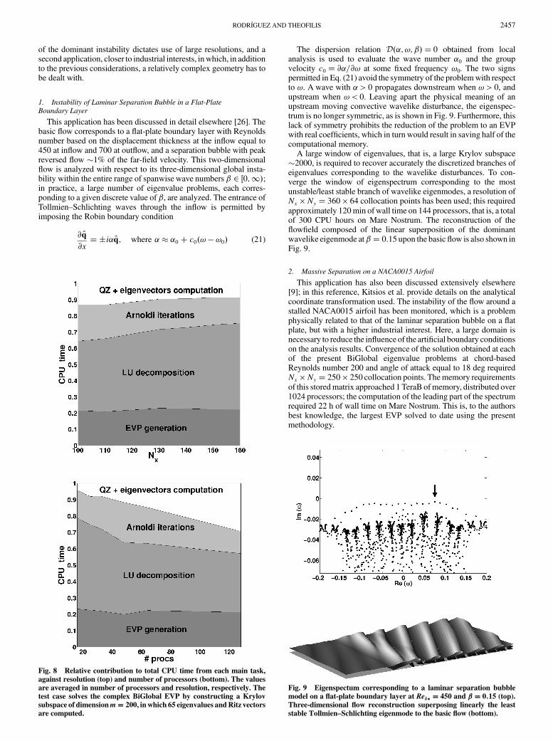
The dispersion relation D!$; !;!# $ 0 obtained from localanalysis is used to evaluate the wave number $0 and the groupvelocity c0 $ @$=@! at some !xed frequency !0. The two signspermitted in Eq. (21) avoid the symmetry of the problemwith respectto !. A wave with $> 0 propagates downstream when ! > 0, andupstream when ! < 0. Leaving apart the physical meaning of anupstream moving convective wavelike disturbance, the eigenspec-trum is no longer symmetric, as is shown in Fig. 9. Furthermore, thislack of symmetry prohibits the reduction of the problem to an EVPwith real coef!cients, which in turn would result in saving half of thecomputational memory.
A large window of eigenvalues, that is, a large Krylov subspace(2000, is required to recover accurately the discretized branches ofeigenvalues corresponding to the wavelike disturbances. To con-verge the window of eigenspectrum corresponding to the mostunstable/least stable branch of wavelike eigenmodes, a resolution ofNx * Ny $ 360 * 64 collocation points has been used; this requiredapproximately 120min of wall time on 144 processors, that is, a totalof 300 CPU hours on Mare Nostrum. The reconstruction of the"ow!eld composed of the linear superposition of the dominantwavelike eigenmode at!$ 0:15 upon the basic "ow is also shown inFig. 9.
2. Massive Separation on a NACA0015 Airfoil
This application has also been discussed extensively elsewhere[9]; in this reference, Kitsios et al. provide details on the analyticalcoordinate transformation used. The instability of the "ow around astalled NACA0015 airfoil has been monitored, which is a problemphysically related to that of the laminar separation bubble on a "atplate, but with a higher industrial interest. Here, a large domain isnecessary to reduce the in"uence of the arti!cial boundary conditionson the analysis results. Convergence of the solution obtained at eachof the present BiGlobal eigenvalue problems at chord-basedReynolds number 200 and angle of attack equal to 18 deg requiredNx * Ny $ 250 * 250 collocation points. Thememory requirementsof this storedmatrix approached 1 TeraB ofmemory, distributed over1024 processors; the computation of the leading part of the spectrumrequired 22 h of wall time on Mare Nostrum. This is, to the authorsbest knowledge, the largest EVP solved to date using the presentmethodology.
Fig. 8 Relative contribution to total CPU time from each main task,against resolution (top) and number of processors (bottom). The valuesare averaged in number of processors and resolution, respectively. Thetest case solves the complex BiGlobal EVP by constructing a Krylovsubspace of dimensionm! 200, inwhich 65 eigenvalues andRitz vectorsare computed.
Fig. 9 Eigenspectum corresponding to a laminar separation bubblemodel on a !at-plate boundary layer at Re"" ! 450 and !! 0:15 (top).Three-dimensional !ow reconstruction superposing linearly the leaststable Tollmien–Schlichting eigenmode to the basic !ow (bottom).
RODRÍGUEZ AND THEOFILIS 2457
A representative eigenspectrum and a "ow reconstruction usingthe dominant wavelike eigenmode at!$ 1 is shown in Fig. 10. Notethat, in contrast with the previous problem, the eigenspectrum is nowsymmetric, in accordance with the fact that the boundary conditionsimposed do not alter the symmetry with respect to !. The instabilityproperties of the two-dimensional basic "ow were shown to beresponsible for the three-dimensionalization of the "ow!eld. In thesnapshot on the !gure, the resultant three-dimensional reversed-"owregion is apparent.
IV. ConclusionsAparallel code has been developed for the solution of large partial-
differential-equation eigenvalue problems resulting from theBiGlobal instability theory. This code employs the dense, parallellinear-algebra library ScaLAPACK, and distributed-memorymachines to circumvent the restrictions in memory and CPU timeimposed by solution of this problem on serial shared-memoryplatforms. A hand-coded parallel version of the Arnoldi algorithmhas been developed, allowing for "exibility, and a detailed study ofthe different parallelization aspects has been performed. Althoughparallelization of the matrix creation and its LU decomposition hasbeen straightforward, the parallel implementation of the Arnoldialgorithm has been rather challenging, especially in terms ofscalability. A solution based on a combination of distributed globaland nondistributed (and then repeated on each processor) arrays hasbeen proposed. Veri!cation and validation of the algorithm wasprovided at low resolutions, by reference to well-studied modelproblems. Convergence of results was obtained at high resolutions,unattainable on serial machines.
Massive parallelization studies have been carried out, using up to1024 processors, on three different platforms. The comparisonbetween thewall-clock times indicates that the performance obtainedby the optimized versions of ScaLAPACK is an order of magnitudebetter than that offered by the free versions of this library. Theexistence of an optimal number of processors at each resolution hasbeen documented and the effect of using an appropriately con-structed processor grid has been demonstrated. At the high end of thenumber of processors used, the detrimental effect of increasing thenumber of processors beyond this optimal has been shown, with an
increase of wall-clock time resulting from overdistribution ofmatrices. At the other extreme of the number of processors, if theminimum number of processors is used to store the global matrix, theresulting wall time is prohibitive for practical applications. A sys-tematic study of the scaling of time with resolution and number ofprocessors has been completed, providing qualitative and quantita-tive predictions for the wall time required; this is expected to beuseful in future studies devoted to physical aspects of BiGlobal"ow instability.
The present methodology has been employed to analyze physicalproblems in which large resolutions are instrumental for the successof the analysis. Concretely, instability results of three-dimensionalwavelike disturbances of reversed-"ow con!gurations, namely alaminar separation bubble on a "at plate and massive separation on aNACA0015 airfoil, were presented as examples of the applications,the global instability of which may be addressed successfully by theproposed enabling technology. Nevertheless, the rather large com-puting resources required for the analysis of "ow instability inrealistic geometries (especially when a large part of the eigenspec-trum must be recovered) points at the need for investigation intoalternative approaches for the eigenspectrum computation; theresults of such efforts will be presented elsewhere.
AcknowledgmentsThe material is based on research sponsored by the U.S. Air Force
Of!ce of Scienti!c Research, Air Force Material Command, underagreement number FA8655-06-1-3066 to Nu modelling s.l., entitledGlobal Instabilities in Laminar Separation Bubbles. The grant ismonitored by Douglas Smith (originally by Rhett Jefferies) of theU.S. Air Force Of!ce of Scienti!c Research and S. Surampudi of theEuropean Of!ce of Aerospace Research and Development. Theviews and conclusions contained herein are those of the author andshould not be interpreted as necessarily representing the of!cialpolicies or endorsements, either expressed or implied, of the U.S. AirForce Of!ce of Scienti!c Research or the U.S. Government. TheU.S. Government is authorized to reproduce and distribute reprintsfor Governmental purposes notwithstanding any copyright notationthereon. Computations have been performed on the CeSViMa andMareNostrum facilities.
References[1] Drazin, P. G., and Reid, W. H., Hydrodynamic Stability, Cambridge
Univ. Press, Cambridge, England, U.K., 1981.[2] Schmid, P., and Henningson, D. S., Stability and Transition in Shear
Flows, Springer, New York, 2001.[3] Theo!lis, V., “Advances in Global Linear Instability Analysis of
Nonparallel and Three-Dimensional Flows,” Progress in AerospaceSciences, Vol. 39, No. 4, 2003, pp. 249–315.doi:10.1016/S0376-0421(02)00030-1
[4] Theo!lis, V., and Colonius, T., “Three-Dimensional Instabilities ofCompressible FlowoverOpenCavities: Direct Solution of theBiGlobalEigenvalue Problem,” AIAA Paper 2004-2544, 2004.
[5] Robinet, J.-C., “Bifurcations in Shock-Wave/Laminar-Boundary-LayerInteraction: Global Instability Approach,” Journal of Fluid Mechanics,Vol. 579, May 2007, pp. 85–112.doi:10.1017/S0022112007005095
[6] Theo!lis, V., Hein, S., and Dallmann, U., “On the Origins of Unsteadi-ness and Three-Dimensionality in a Laminar Separation Bubble,”Philosophical Transactions of the Royal Society of London, Series A:Mathematical and Physical Sciences, Vol. 358, No. 1777, 2000,pp. 3229–3324.doi:10.1098/rsta.2000.0706
[7] Ehrenstein, U., and Gallaire, F., “On Two-Dimensional TemporalModes in Spatially Evolving Open Flows: The Flat-Plate BoundaryLayer,” Journal of FluidMechanics, Vol. 536, Aug. 2005, pp. 209–218.doi:10.1017/S0022112005005112
[8] Åkervik, E., Ehrenstein, U., Gallaire, F., and Henningson, D., “GlobalTwo-Dimensional StabilityMeasures of the Flat-Plate Boundary-LayerFlow,”European Journal ofMechanics, B: Fluids, Vol. 27, No. 5, 2008,pp. 501–513.doi:10.1016/j.euromech"u.2007.09.004
[9] Kitsios, V., Rodríguez, D., Theo!lis, V., Ooi, A., and Soria, J.,
Fig. 10 Eigenspectum corresponding toNACA0015 airfoil atRe! 200and !! 1 (top). Three-dimensional !ow reconstruction superposinglinearly the least stable eigenmode to the basic !ow (bottom).
“BiGlobal Instability Analysis of Turbulent Flow over an Airfoil at anAngle of Attack,” AIAA Paper 2008–4384, 2008.
[10] Edwards,W. S., Tuckerman, L. S., Friesner, R. A., and Sorensen, D. C.,“Krylov Methods for the Incompressible Navier–Stokes Equations,”Journal of Computational Physics, Vol. 110, No. 1, 1994, pp. 82–102.doi:10.1006/jcph.1994.1007
[11] Barkley, D., Gomes, M. G. M., and Henderson, R. D., “Three-Dimensional Instability in a Flow over a Backward-Facing Step,”Journal of Fluid Mechanics, Vol. 473, Dec. 2002, pp. 167–190.
[12] Bagheri, S., Åkervik, E., Brandt, L., and Henningson, D. S., “Matrix-Free Methods for the Stability and Control of Boundary Layers,” AIAAJournal, Vol. 47, No. 5, 2009, pp. 1057–1068.doi:10.2514/1.41365
[13] Blackford, L. S., Choi, J., Cleary, A., E. D’Azeuedo, J. Demmel, and I.Dhillon et al., ScaLAPACK User’s Guide, Society for Industrial andApplied Mathematics, Philadelphia, PA, 1997, ISBN 0-89871-397-8.Petitet, A., Whaley, R. C., Demmel, J., Dhillon, I., Stanley, K.,Dongarra, J., Hammarling, S., Henry, G., and Walker, D.,“ScaLAPACK: A Portable Linear Algebra Library for DistributedMemory Computers: Design Issues and Performance,” 1996.
[14] Borrill, J., “MADCAP: The Microwave Anositropy Dataset Computa-tional Analysis Package,” Proceedings of the 5th European SGI/CrayMPP Workshop, 1999, http://arxiv.org/abs/astro-ph/9911389v1.
[15] Bonoli, P., Batchelor, D., Berry, L., Choi,M., D’Ippolito, D.A., Harvey,R.W., Jaeger, E. F., Myra, J. R., Phillips, C. K., Smithe, D. N., Tang, V.,Valeo, E., Wright, J. C., Brambilla, M., Bilato, R., Lancellotti, V., andMaggiora, R., “Evolution ofNonthermal ParticleDistributions in RadioFrequencyHeating of Fusion Plasmas,” Journal of Physics: ConferenceSeries, Vol. 78, 2007, p. 012006.doi:10.1088/1742-6596/78/1/012006
[16] Macaraeg, M., Streett, C., and Hussaini, M., A Spectral CollocationSolution to the Compressible Stability Eigenvalue Problem, NASA,TR TP-2858, 1988.
[17] Malik, M. R., “Numerical Methods for Hypersonic Boundary LayerStability,” Journal of Computational Physics, Vol. 86, No. 2, 1990,
pp. 376–413.doi:10.1016/0021-9991(90)90106-B
[18] Theo!lis, V., Journal of Engineering Mathematics, Vol. 34,Nos. 1–21998, pp. 111–129.doi:10.1023/A:1004366529352
[19] Canuto, C., Hussaini, M. Y., Quarteroni, A., and Zang, T. A., SpectralMethods: Fundamentals in SingleDomains, Springer, NewYork, 2006.
[20] de Vicente, J., Valero, E., and Theo!lis, V., “Numerical Considerationsin Spectral Multidomain Methods for BiGlobal Instability Analysis ofOpen Cavity Con!gurations,” Progress in Industrial Mathematics atECMI 2006, Springer, New York, 2006, ISBN 9783540719922.
[21] Golub, G. H., and Van Loan, C. F.,Matrix Computations, 2nd ed., JohnHopkins Univ. Press, Baltimore, MD, 1989, ISBN 0-8018-3739-1.
[22] Saad, Y., “Variations of Arnoldi’s Method for Computing Eigenele-ments of Large Unsymmetric Matrices,” Linear Algebra and ItsApplications, Vol. 34, No. 1, 1980, pp. 269–295.doi:10.1016/0024-3795(80)90169-X
[23] Theo!lis, V., “On Instability Properties of Incompressible LaminarSeparation Bubbles on a Flat Plate Prior to Shedding,” AIAAPaper 2007-0540, 2007.
[24] Tatsumi, T., and Yoshimura, T., “Stability of the Laminar Flow in aRectangular Duct,” Journal of Fluid Mechanics, Vol. 212, No. 1, 1990,pp. 437–449.doi:10.1017/S002211209000204X
[25] Theo!lis, V., Duck, P. W., and Owen, J., “Viscous Linear StabilityAnalysis of Rectangular Duct and Cavity Flows,” Journal of FluidMechanics, Vol. 505, April 2004, pp. 249–286.doi:10.1017/S002211200400850X
[26] Rodríguez, D., and Theo!lis, V., “On Instability and StructuralSensitivity of Incompressible Laminar Separation Bubbles in a Flat-Plate Boundary Layer,” AIAA Paper 2008–4148, 2008.


![MINISTRY OF LABOUR AND EMPLOYMENT NOTIFICATION of Wages 24000.pdfEXTRAORDINARY II— — (ii) PART II—Section 3—Sub-section (ii) PUBLISHED BY AUTHORITY 2459] No. 2459] NEW DELHI,](https://static.documents.pub/doc/80x56/5e7bdb89f65cd9392d795a64/ministry-of-labour-and-employment-notification-of-wages-24000pdf-extraordinary.jpg)


