From continuous to discrete and finite Gabor frames Mads Sielemann Jakobsen Academic advisors: Ole Christensen Jakob Lemvig August 31, 2013 A dissertation submitted to the department of Applied Mathematics and Computer Science at the Technical University of Denmark in partial fulfilment of the M.Sc. degree
Transcript
From continuous to discrete and finite Gabor frames
Mads Sielemann Jakobsen
Academic advisors:
Ole ChristensenJakob Lemvig
August 31, 2013
A dissertation submitted to the department ofApplied Mathematics and Computer Science
at the Technical University of Denmarkin partial fulfilment of the M.Sc. degree
Abstract
This master thesis is concerned with the transition of Gaborframes and their duals from L2(R) to the discrete and finite set-ting in `2(Z) and Cd. The existing literature by Janssen andSøndergaard on this topic is examined in detail. Their resultsconcerning dual systems are based on the structure of the cano-nical dual and the Wexler-Raz relations. We present a new ap-proach to the topic by considering the characterizing equationsfor dual Gabor generators, which exist for both L2(R) and Cd.Based on the similarity of these equations, we formulate newresults on the sampling of dual pairs of Gabor generators fromL2(R) to Cd.The new approach naturally extends to types of frames whichalso feature characterizing equations of a similar form as dualGabor generators. Such frame types include shift-invariant andwavelet systems, for which we show preliminary results.New constructions of explicit dual Gabor generators in L2(R)are also presented in the thesis. Specifically, we modify proofsof results due to Christensen and Kim. These modifications yieldnew constructions of explicit dual pairs under the partition ofunity condition. We also present a result assuming the new“alternating” partition of unity condition.Furthermore, the thesis includes introductory sections concern-ing abstract harmonic analysis on locally compact and Abeliangroups, frame theory in Hilbert spaces and Gabor analysis.
i
Resume
Dette speciale omhandler overføringen af Gabor systemer ogderes duale fra L2(R) til det diskrete og finite tilfælde i `2(Z)og Cd. Den eksisterende litteratur af Janssen og Søndergaardomkring dette emne bliver indgaende undersøgt. Deres resul-tater angaende duale systemer baserer sig pa strukturen af denkanoniske dual og Wexler-Raz relationerne. I dette specialevælges der en anden angrebsvinkel, nemlig karakteriserings lig-ningerne for duale par af Gabor generatorer som eksisterer badefor L2(R) og Cd. Vi udnytter ligningernes ensartethed til atformulere nye resultater omkring overføringen af duale par afGabor generatorer fra L2(R) til Cd.Den nye tilgang kan naturligt overføres til andre typer af frames,som ogsa har karakteriserende ligninger i stil med duale Gaborgeneratorer. Sadanne frames indebærer bl.a. shift-invariante ogwavelet systemer, for hvilke der ogsa præsenteres resultater.Nye konstruktioner af eksplicite duale par af Gabor generatorerbliver ogsa fremført i specialet. Der modificeres beviser af resul-tater af Christensen og Kim, som giver nye konstruktioner un-der den velkendte “partition og unity”-betingelse. Der præsen-teres ligeledes et resultat under den nye “alternating partitionof unity”-betingelse.Derudover indeholder afhandlingen introducerende afsnit omkringabstrakt harmonisk analyse pa lokalt kompakte Abelske grup-per, frame teori i Hilbert rum og Gabor analyse.
ii
Notation
• N = {1, 2, 3, . . . } – the set of natural numbers
• N0 = {0, 1, 2, 3, . . . } – the set of natural numbers including zero.
• Z = {0,±1,±2, . . . } – the set of integers.
• R – the set of real numbers.
• R+ – the set of positive real numbers, {x ∈ R : x > 0}.
• R+0 – the set of non-negative real numbers, {x ∈ R : x ≥ 0}.
• C – the set of complex numbers.
• i – the imaginary unit, i2 = −1.
• z = a− ib – the complex conjugate of z = a+ ib ∈ C, a, b ∈ R.
• T – the torus, {z ∈ C : |z| = 1}. We identify T with the interval [0, L[ by associatingthe number x ∈ [0, L[ with the complex number e2πix/L.
• Zd = Z/dZ for d ∈ N – the set of integers modulo d.
• δk – the Kronecker delta, δk = 1 if k = 0. If k 6= 0 then δk = 0.
• dxe – the smallest integer k ∈ Z for which x ≤ k.
• bxc – the largest integer k ∈ Z for which x ≥ k.
• G – a locally compact and Abelian group.
• G – the dual group of G.
• ω, χ – elements of a dual group G.
•∫X f(x) dµG(x) – the Haar integral of an integrable function f over the set X ⊆ G.
• H – a separable Hilbert space.
• Cc(R) – the set of functions {f : R→ C : f is continuous and has compact support}.
• 〈·, ·〉H – the inner product w.r.t. the Hilbert space H. The subscript is left out if it isclear which inner product is used.
• U∗ – the adjoint operator of a linear and bounded operator U : H1 → H2.
• F – the Fourier transform operator.
iii
• f – the Fourier transform of a function f .
• Ta – the translation operator, see Definition 2.1.
• Eb – the modulation operator, see Definition 2.1.
• Dc – the dilation operator, see Definition 2.5.
• s.t. – acronym for such that.
• ONB – acronym for orthonormal basis.
• w.l.o.g. – acronym for without loss of generality.
•(nk
)– binomial coefficient, n over k, defined as
(nk
):= n!
k!(n−k)! .
• lcm(a, b) – the least common multiple of a and b.
1 IntroductionThis master thesis was written over five months, from the beginning of April to the end ofAugust in 2013. It resembles the workload of 30 ECTS points and is a partial fulfilmentof the Master of Science degree at the department of Applied Mathematics and ComputerScience at the Technical University of Denmark.
The reader is expected to have knowledge of Normed Vector spaces, Hilbert spaces andfunctional analysis. The knowledge of Fourier analysis on locally compact Abelian (LCA)groups is not necessary, yet it gives fundamental insight into the overall picture of Fourierand Gabor theory on, e.g., the classical LCA groups L2(R), L2([0, L]), `2(Z) and Cd. Simi-larly, knowledge on measure theory is not needed for the majority of the thesis, however, itis necessary to the understanding of all details in Section 4.1. Some results in this thesis areconcerned with functions of the Feichtinger algebra S0(R). We give the definition and statekey properties in Section 4.2. For a detailed introduction and more properties of S0(R) werefer to [13], [15] and [22].
In Section 2 a brief introduction to harmonic analysis on locally compact Abelian groupsis given, furthermore we present results with proofs concerning the translation and modula-tion operators. With these operators in hand we define Gabor systems on the classical LCAgroups L2(R), L2([0, L]), `2(Z) and Cd. In Section 3 we introduce frame theory on Hilbertspaces, in particular results concerning dual frames and Gabor frames are presented. If thereader is well aware of frame and Gabor theory on the classical LCA groups, then Section2 and 3 can be skipped and used as reference for specific results in the later sections.
Section 4 and 5 represent the main body of work in the thesis. In these sections we gothrough literature and new results concerning sampling and periodization of Gabor frames.We begin Section 4 by presenting the content of [20] and [34]. An overview over the results isgiven in the beginning of Section 4. The results in the first mentioned article are especiallylengthy, as the theory requires details and technicalities. In Section 5 we present a newapproach to the topics addressed in [20] and [34] and in fact improve some of the knownresults. Both sections include examples in which the results are applied to explicit dualpairs.
In Section 6 we show how the new approach from Section 5 can be applied to shift-invariantand wavelet systems. In fact, we show a preliminary result on sampling dual shift-invariantframes in L2(R) to obtain dual shift-invariant frames in Cd. For wavelet systems the issueis more complicated, since there does not exist a dilation operator on Cd in the literature.Yet, we present a definition of certain dilation-like operators and wavelet-like systems in Cd,for which we indeed find characterization equations of dual frames matching known resultsin L2(R)!
Finally, in Section 7 new explicit constructions of dual Gabor frame generators for L2(R)are presented. Specifically, we work on the well known partition of unity condition and alsointroduce the new so-called “alternating” partition of unity condition.
1
Appendix A is concerned with the proofs of the duality conditions in Cd for Gabor, shift-invariant and wavelet-like systems. These conditions are presented in Theorem 3.20, 6.3and 6.12, respectively. Appendix B contains a lemma concerning Lebesgue points, whichis needed in the proof of Proposition 4.6. Appendix C is concerned with the multinomialtheorem and notation which is used in Section 7.
I would like to thank my supervisors Ole Christensen & Jakob Lemvig and also my fellowstudent Lasse Hjuler Christiansen for many interesting discussions of various topics relatedto the contents of this thesis.
Mads S. JakobsenLyngby, August 2013.
2
2 Theory on locally compact Abelian groupsIn this section we present the theory of Fourier analysis on locally compact Abelian (LCA)groups. The following is a short review only, and it is not intended as a complete explanationof the subject. We refer to the books [14] and [17] for far more complete descriptions of thetheory of Harmonic analysis on LCA groups. We also present results with proofs concerningthe translation and modulation operator and their commutator relations with the Fouriertransform. With these operators in hand, we define Gabor systems on some LCA groups inSection 2.1.
In the following G will always denote a locally compact Abelian group. As prime examplesof such groups we mention R,T,Z and Zd. To each locally compact group we associate itsdual group G – the set of all continuous group homomorphisms mapping from G into thetorus T. The dual group G is again locally compact and Abelian, furthermore, the dual ofG has the property that G ∼= G, that is, there exists a homeomorphic group isomorphismfrom G onto G.
Recall that on locally compact groups we can define the so-called Haar measure µ. Usingthis measure, we define the Lp-spaces in the usual way: for p ≥ 1 define
Lp(G) := {f : G→ C |∫G|f(x)|p dµ(x) <∞}.
For two functions f, g ∈ L2(G) we define the inner product
〈f, g〉 :=∫Gf(x)g(x) dµ(x). (2.1)
The space L2(G) together with the inner product defined in (2.1) is a Hilbert space.To each function f in L1(G) we can define its Fourier transform, which is a new function
f : G→ C given by
(Ff)(ω) = f(ω) :=∫Gf(x)ω(x) dµ(x), ω ∈ G. (2.2)
If f ∈ L1(G), then f can be reconstructed from f by the inverse Fourier transform
f(x) = (F−1f)(x) :=∫Gf(ω)ω(x) dµ(ω), x ∈ G.
The Fourier transform can be extended to a unitary mapping from L2(G) onto L2(G),which we also denote by F . From the above abstract definition of the Fourier transform onecan deduce the classical continuous Fourier transform (G = R), the Fourier series (G = T)and the discrete Fourier transform (G = Zd).
Concerning the classical LCA groups R,T,Z and Zd we mention the following result abouttheir respective dual group:
• R ∼= R, R = {χ : R→ T |χ(x) = e2πixγ, γ ∈ R};
3
• T ∼= Z, T = {χ : T→ T |χ(z) = zn, n ∈ Z};
• Z ∼= T, Z = {χ : Z→ T |χ(n) = zn, z ∈ T};
• Zd ∼= Zd, Zd = {χ : Zd → T |χ(k) = e2πink/d, n ∈ Zd}.
We refer to [14] and [17] for more on this subject. Recently the LCA group of the p-adicnumbers Qp has also found interest in engineering, quantum mechanics, and also the con-struction of wavelets systems and multiresolution analysis on L2(Qp). We refer to [14], [23],[24] and [25].
On an LCA group we can define the translation and modulation operators. They are es-sential for the definition of Gabor (Weyl-Heisenberg) systems. To emphasize the distinctionbetween this theory compared to, e.g., L2(R), we use multiplication as group operation anddenote the inverse of x ∈ G by x−1.
Definition 2.1 Let G be an LCA group and define the following operators on L2(G).
• For a ∈ G, the operator Ta, called translation by a, is defined by
Ta : L2(G)→ L2(G), (Taf)(x) := f(xa−1), x ∈ G.
• For χ ∈ G, the operator Eχ, called modulation by χ, is defined by
Eχ : L2(G)→ L2(G), (Eχf)(x) := χ(x)f(x), x ∈ G.
By translation invariance of the Haar measure and a change of variables y = xa−1, we havethat ∫
G|Taf(x)|2 dµ(x) =
∫G|f(xa−1)|2 dµ(x) =
∫G|f(y)|2 dµ(y) <∞. (2.3)
Thus Ta indeed maps from L2(G) into L2(G).A similar calculation for Eb shows that∫
G|Eχf(x)|2 dµ(x) =
∫G|χ(x)f(x)|2 dµ(x) =
∫G|f(x)|2 dµ(x) <∞. (2.4)
Here we have used that for all χ ∈ G is by definition |χ(x)| = 1. Equation (2.4) shows thatEχ maps from L2(G) into L2(G).
Remark 2.2 From Definition 2.1 together with Pontryagin Theorem (see [14] or [17]) fol-lows that modulation of a function in L2(G) is given as follows:
• For b ∈ G, the operator Eb, called modulation by b, is given by
Eb : L2(G)→ L2(G), (Ebφ)(ω) := ω(b)φ(ω), ω ∈ G.
4
We now turn to some of the properties of the translation and modulation operator. Theauthor has not seen the results in Proposition 2.3 and 2.4 in the literature, yet they are wellknown on L2(R) and the following results are therefore natural to formulate in the settingof LCA groups. For the corresponding results on L2(R), see for example [5, Section 6.2].
Proposition 2.3 The operators Ta and Eχ are linear, unitary operators of L2(G) ontoL2(G). Moreover,
(i) T−1a = Ta−1 = (Ta)∗ ;
(ii) E−1χ = Eχ−1 = (Eχ)∗.
Proof. Let us first prove the statements for Ta. Let f ∈ L2(G).For α, β ∈ C and f, g ∈ L2(G), we have
Eχ−1Eχf(x) = χ−1(x)χ(x)f(x) = χ(x)χ(x)f(x) = f(x) .We have now shown E−1
χ = Eχ−1 = E∗χ, that the operator Eχ is unitary and indeed mapsonto L2(G). �
Similar to the classical theory of Fourier analysis on L2(R), the operators F , Eχ and Taenjoy a set of commutator relations. These play an essential role in time-frequency (Gabor)analysis.
Proposition 2.4 The translation and modulation operator together with the Fourier trans-form satisfy the following relationships. Let a ∈ G and χ ∈ G, then for all f ∈ L2(G)
(i) (TaEχf)(x) = χ(a−1)(EχTaf)(x) ;
(ii) (FTaf)(ω) = (Ea−1Ff)(ω), that is FTa = Ea−1F ;
(iii) (FEχf)(ω) = (TχFf)(ω), that is FEχ = TχF .
Proof. (i). Using that χ ∈ G is a group homomorphism, then by the definition of theoperators we have that
(ii). Using a change of variables, the fact that elements in G are group homomorphismsand the fact that ω = ω−1, ω−1(a) = ω(a−1) for ω ∈ G, we have that for all f ∈ L1(G)
(FTaf)(ω) =∫G
(Taf)(x)ω(x) dµ(x) =∫Gf(xa−1)ω(x) dµ(x)
=∫Gf(y)ω(y)ω(a) dµ(y) = ω(a)
∫Gf(y)ω(y) dµ(y)
= ω−1(a)(Ff)(ω) = ω(a−1)(Ff)(ω) = (Ea−1Ff)(ω).
Since L1(G) ∩ L2(G) is dense in L2(G) (see [17]), the result extends to all functions inL2(G).
6
(iii). Using the definition of the group operation and inversion in G together with thedefinition of the Fourier transform, yields that for all f ∈ L1(G)
As in (ii) the result extends to all functions in L2(R). �
Before we turn to the definition of Gabor systems, we define another important operatoron L2(R).
Definition 2.5 For c > 0, the operator Dc, called dilation by c, is defined by
Dc : L2(R)→ L2(R), (Dcf)(x) := c−1/2f(x/c), x ∈ R. (2.7)
The dilation operator has the following properties:
Proposition 2.6 The operator Dc is a linear, bounded and unitary operator from L2(R)onto L2(R). Moreover, together with the translation, modulation and Fourier transform onL2(R) the dilation operator satisfies
(i) D−1c = D1/c = (Dc)∗ ;
(ii) TaDc = DcTa/c ;
(iii) DcEb = Eb/cDc ;
(iv) FDc = D1/cF .
Proof. The results can be shown by similar calculations as in the proofs of Proposition2.3 and 2.4. The results are also stated in, e.g., [3, Section 2.9]. �
7
2.1 Gabor systemsWith the translation and modulation operators in hand we will now define Gabor systems.A Gabor system is a family of functions in L2(G), which is generated from one functiong ∈ L2(G) in a special way: the Gabor system is constructed by translating the generatorg in the time-frequency domain on a lattice Λ ⊆ G × G. The function g is also called thewindow function. Formally, the Gabor system generated by g is defined as the set
{EχTag}(a,χ)∈Λ.
In the literature Gabor systems are also called Weyl-Heisenberg systems. By Proposition2.4(iii) we find that
FEχTag = TχFTag, ∀g ∈ L2(G),
so indeed, a Gabor system consists of translates in time and frequency of the function g. Inthis text we shall only consider so-called regular Gabor systems in the LCA groups R,Z, [0, L]and Zd, which are described below. These are systems, for which the lattice Λ is of the formΛ = (an, χm) for fixed (a, χ) ∈ G × G and n,m are from “some” subset of Z. This subsetdepends on the properties of the group at hand. For more on Gabor analysis on LCA groups,see Chapter 6 and 7 in [13] by Grochenig, Feichtinger and Kozek.
2.1.1 Gabor systems in L2(R)
On the space L2(R) the translation and modulation operators take the following form:
• For a ∈ R, the operator Ta, called translation by a, is defined by
Ta : L2(R)→ L2(R), (Taf)(x) := f(x− a), x ∈ R.
• For b ∈ R, the operator Eb, called modulation by b, is defined by
Eb : L2(R)→ L2(R), (Ebf)(x) := e2πibxf(x), x ∈ R.
With these operators at hand, let g ∈ L2(R) and a, b > 0, then the Gabor system generatedby g with translation parameter a and modulation parameter b is the family of functions ofthe form
{EmbTnag}m,n∈Z.
Specifically, we have that
(EmbTnag)(x) = e2πimbxg(x− na), x ∈ R.
8
2.1.2 Gabor systems in L2([0, L])
On the space of L-periodic functions L2([0, L]), the translation and modulation operatorstake the following form:
• For a ∈ [0, L], the operator Ta, called translation by a, is defined by
Ta : L2([0, L])→ L2([0, L]), (Taf)(x) := f(x− a), x ∈ [0, L].
• For b ∈ Z, the operator Eb, called modulation by b, is defined by
Let now g ∈ L2([0, L]), choose a ∈ [0, L] such that there exists an N ∈ N with aN = L andlet b ∈ Z. The Gabor system generated by g with translation parameter a and modulationparameter b is the family of functions of the form
{EmbTnag}N−1n=0,m∈Z.
Specifically, we have that
(EmbTnag)(x) = e2πimb/Lg(x− na), x ∈ [0, L[.
2.1.3 Gabor systems in `2(Z)
On the sequence space `2(Z), the translation and modulation operators take the followingform:
• For a ∈ Z, the operator Ta, called translation by a, is defined by
Ta : `2(Z)→ `2(Z), (Taf)(x) := f(x− a), x ∈ Z.
• For b ∈ [0, 1[, the operator Eb, called modulation by b, is defined by
Eb : `2(Z)→ `2(Z), (Ebf)(x) := e2πibxf(x), x ∈ Z.
Let now g ∈ `2(Z), a ∈ Z and choose b ∈ [0, 1[ such that there exists an M ∈ N withbM = 1. The Gabor system generated by g with translation parameter a and modulationparameter b is the family of functions of the form
{EmbTnag}M−1m=0,n∈Z.
Specifically, we have that
(EmbTnag)(x) = e2πimbxg(x− na).
9
2.1.4 Gabor systems in Cd
On the finite discrete space Cd, d ∈ N, the translation and modulation operators take thefollowing form:
• For a ∈ Zd, the operator Ta, called translation by a, is defined by
Ta : Cd → Cd, (Taf)(x) := f(x− a), x ∈ Zd.
• For b ∈ Zd, the operator Eb, called modulation by b, is defined by
Eb : Cd → Cd, (Ebf)(x) := e2πibx/df(x), x ∈ Zd.
Let g ∈ Cd and choose a, b ∈ Zd such that there exists M,N ∈ N with aN = bM = d.The Gabor system generated by g with translation parameter a and modulation parameterb is the family of functions of the form
{EmbTnag}M−1,N−1m=0,n=0 .
Specifically, we have that
(EmbTnag)(x) = e2πimbx/dg(x− na).
10
3 Frames in Hilbert spacesIn this section we introduce frames in Hilbert spaces. Frames are sequences that havesimilar properties as orthonormal bases for Hilbert spaces. The aim is to present the basicproperties and results concerning frames and their duals. We give proofs for most of theresults, however in a few cases more technicalities are needed, the details of which can befound in [3].
We begin with the definition of a frame.
Definition 3.1 (Frame) Let {fk}∞k=1 be a sequence of elements in H. The sequence {fk}∞k=1is a frame for H if there exist constants 0 < A ≤ B <∞ such that
A‖f‖2 ≤∞∑k=1|〈f, fk〉|2 ≤ B‖f‖2, ∀f ∈ H. (3.1)
We call
A‖f‖2 ≤∞∑k=1|〈f, fk〉|2, ∀f ∈ H and
∞∑k=1|〈f, fk〉|2 ≤ B‖f‖2, ∀f ∈ H
the lower and the upper frame condition, respectively. If a sequence satisfies the upper framecondition, it is called a Bessel sequence. The constants A and B are called frame bounds.The upper frame bound B is also called the Bessel bound of the sequence {fk}∞k=1.
Remark 3.2 If one can verify the existence of frame bounds for all functions in a densesubset of H, then the sequence {fk}∞k=1 is a frame. This follows from [3, Lemma 5.1.2]
A special frame, a so-called tight frame, is achieved if the frame bounds coincide, i.e., ifA = B.
Definition 3.3 (Tight frame) A sequence {fk}∞k=1 in H is a tight frame if there exists aconstant A > 0 such that
∞∑k=1|〈f, fk〉|2 = A‖f‖2, ∀f ∈ H. (3.2)
Remark 3.4 The frame inequality in (3.1) and tight frame equality (3.2) can be viewedas a generalization of the Parseval equality for orthonormal bases, which states that if asequence {ek}∞k=1 is an orthonormal basis for a Hilbert space H, then
∞∑k=1|〈f, ek〉|2 = ‖f‖2.
Hence, an orthonormal basis is a tight frame with frame bound A = 1.
11
We will now show that frames share the most important property of an orthonormalbasis, namely that every element in the Hilbert space can be written as an infinite linearcombination of the frame elements. To show this, we associate two operators to each frame.These will play an important role in the formulation of the main result concerning framesin Theorem 3.8.
Proposition 3.5 Let {fk}∞k=1 be a frame in a Hilbert space H. Then
T : `2(N)→ H, T{ck}∞k=1 :=∞∑k=1
ckfk (3.3)
defines a linear and bounded operator on H with ‖T‖ ≤√B. Moreover, the adjoint operator
T ∗ : H → `2(N) is given by
T ∗f ={〈f, fk〉
}∞k=1
, ∀f ∈ H.
Remark 3.6 We call T the synthesis and T ∗ the analysis operator of the frame {fk}∞k=1.
Proof. We first show that T is well defined, i.e., for any {ck}∞k=1 ∈ `2(N) the infinite sum
T{ck}∞k=1 =∞∑k=1
ckfk
actually converges. Take therefore m,n ∈ N with m > n. Then
‖m∑k=1
ckfk −n∑k=1
ckfk‖ = ‖m∑
k=n+1ckfk‖. (3.4)
Recall that in a Hilbert space the norm can be recovered from inner-products by the formula
‖f‖ = sup‖g‖=1
|〈f, g〉|.
Using this on the right hand side in (3.4) followed by an application of the triangle inequality,we have that
‖m∑k=1
ckfk −n∑k=1
ckfk‖ = sup‖g‖=1
|〈m∑
k=n+1ckfk, g〉| = sup
‖g‖=1|
m∑k=n+1
ck〈fk, g〉|
≤ sup‖g‖=1
m∑k=n+1
|ck| |〈fk, g〉|.
Then, by Cauchy-Schwarz’ inequality, we get that
‖m∑k=1
ckfk −n∑k=1
ckfk‖ ≤ sup‖g‖=1
( m∑k=n+1
|ck|2)1/2( m∑
k=n+1|〈fk, g〉|2
)1/2
≤( m∑k=n+1
|ck|2)1/2
sup‖g‖=1
‖g‖√B =
( m∑k=n+1
|ck|2)1/2√
B.
(3.5)
12
In the last step we used that {fk}∞k=1 satisfies the upper frame inequality, where the upperframe bound is denoted by B. In the far right hand side of (3.5) the sum (∑m
k=n+1 |ck|2)1/2
converges to zero as n → ∞, since {ck}∞k=1 ∈ `2(N). We conclude that {∑nk=1 ckfk}∞n=1 is a
Cauchy sequence in the Hilbert space H and thus converges. This shows that the operatorT in (3.3) is well defined.
We now turn to linearity and let α, β ∈ C and {ck}∞k=1, {dk}∞k=1 ∈ `2(N). Then
T{αck + βdk}∞k=1 =∞∑k=1
(αck + βdk)fk = α∞∑k=1
ckfk + β∞∑k=1
dkfk
= αT{ck}∞k=1 + βT{dk}∞k=1.
We conclude that T is a linear operator. To show that T is bounded we use the sameapproach as in (3.5).
‖Tf‖ = ‖∞∑k=1
ckfk‖ ≤ sup‖g‖=1
( ∞∑k=1|ck|2
)1/2( ∞∑k=1|〈fk, g〉|2
)1/2≤√B ‖{ck}∞k=1‖.
In the last step we used the fact that {fk}∞k=1 is a frame in H with upper frame bound B.This shows that T is a linear and bounded operator with ‖T‖ ≤
√B. Since T is linear and
bounded, the adjoint operator T ∗ : H → `2(N) exists, which is linear and bounded as well.Moreover, by definition T ∗ satisfies
Since T ∗ maps into `2(N), every coordinate function is bounded from H to C. It followsfrom Riesz’ representation theorem that
T ∗f = {〈f, gk〉}∞k=1 for some {gk}∞k=1 in H.
By properties of the inner product and (3.6), we conclude that
T ∗f = {〈f, fk〉}∞k=1.
�
The composition of T with T ∗ yields the so-called frame operator
S : H → H, Sf = TT ∗f =∞∑k=1〈f, fk〉fk.
Some of the well-known properties of S are listed in the lemma below. We refer to [3] forthe proof.
Lemma 3.7 (Lemma 5.1.6 in [3]) Let {fk}∞k=1 be a frame with frame operator S andframe bound 0 < A ≤ B. Then the following holds:
13
(i) S is linear, bounded, invertible and self-adjoint.
(ii) {S−1fk}∞k=1 is a frame with frame operator S−1 and frame bounds 0 < B−1 ≤ A−1.
In Theorem 3.8 we present one of the most important results in frame theory. It showsthat every element in the Hilbert space can be written as an infinite linear combination ofthe frame elements. This is a key feature that frames share with bases, which, together withother properties, makes them interesting in, e.g., engineering.
Theorem 3.8 (Theorem 5.1.7 in [3]) Let {fk}∞k=1 be a frame with frame operator S, then
f =∞∑k=1〈f, S−1fk〉fk, ∀f ∈ H
andf =
∞∑k=1〈f, fk〉S−1fk, ∀f ∈ H.
Both series converge unconditionally for all f ∈ H.
Remark 3.9 The sequence {S−1fk}∞k=1 is called the canonical dual frame of {fk}∞k=1.
Proof. In the following we use the properties of S from Lemma 3.7. For f ∈ H we havethat
f = SS−1f =∞∑k=1〈S−1f, fk〉fk =
∞∑k=1〈f, S−1fk〉fk.
And similarlyf = S−1Sf = S−1
∞∑k=1〈Sf, fk〉fk =
∞∑k=1〈f, Sfk〉S−1fk.
Note that the property of being a Bessel sequence is invariant under any rearrangement of theelements in the sequence. The convergence in the above equations is therefore unconditional.�
In order to apply Theorem 3.8 one needs to find S−1 or, at least, {S−1fk}∞k=1. In general,calculating the inverse S−1 is a non-trivial task. As the following result shows, this issue isnon-existent for tight frames.
Corollary 3.10 If {fk}∞k=1 is a tight frame with frame bound A, then the canonical dualframe is {A−1fk}∞k=1 and
f = 1A
∞∑k=1〈f, fk〉fk, ∀f ∈ H.
14
Proof. Using the definition of S, we have for all f ∈ H
〈Sf, f〉 =⟨ ∞∑k=1〈f, fk〉, f
⟩=∞∑k=1〈f, fk〉〈fk, f〉 =
∞∑k=1|〈f, fk〉|2 = A‖f‖2 = A〈f, f〉 = 〈Af, f〉.
Reading from left to right, we find that 〈Sf, f〉 = 〈Af, f〉. If H is a complex Hilbert space,then this implies that S = AI. If H is a real vector space, then since S is self-adjoint,we again conclude that S = AI. Thus, in any case, the frame operator S is the identityoperator on H multiplied with the frame constant A. We conclude that S−1 = A−1I and
f = S−1Sf = 1A
∞∑k=1〈f, fk〉fk.
�
Theorem 3.8 and Corollary 3.10 may give the impression that the canonical dual frame{S−1fk}∞k=1 is the only frame {gk}∞k=1 such that
f =∞∑k=1〈f, gk〉fk, ∀f ∈ H. (3.7)
However, this is not true. To show this we need a definition.
Definition 3.11 We say that a frame is overcomplete, if there exists a non-trivial, possiblyinfinite, linear combination of frame elements that equals zero. That is, a frame {fk}∞k=1 isovercomplete if
∃ {ck}∞k=1 ∈ `2(N)\{0} s.t.∞∑k=1
ckfk = 0.
Theorem 3.12 (Theorem 5.2.3 in [3]) Let {fk}∞k=1 be an overcomplete frame. Thenthere exist frames {gk}∞k=1 6= {S−1fk}∞k=1 for which
f =∞∑k=1〈f, gk〉fk, ∀f ∈ H. (3.8)
Remark 3.13 All frames {gk}∞k=1 for which (3.8) holds are called dual frames of {fk}∞k=1.
Proof. The proof is divided into two cases. (i) Assume fl = 0 for some l ∈ N. By Lemma3.7 the operator S−1 is linear, thus S−1fl = 0. Define now gk = S−1fk for k 6= l and let glbe an arbitrary non-zero vector in H, then for all f ∈ H
∞∑k=1〈f, gk〉fk =
∞∑k=1k 6=l
〈f, S−1fk〉fk + 〈f, gl〉fl︸ ︷︷ ︸=0 since fl=0
=∞∑k=1k 6=l
〈f, S−1fk〉fk =∞∑k=1〈f, S−1fk〉fk = f.
Hence (3.8) holds for {gk}∞k=1 6= {S−1fk}∞k=1.
15
(ii) Assume now fk 6= 0 for all k ∈ N. By assumption
∃{ck}∞k=1 ∈ `2(N) \ {0} s.t.∞∑k=1
ckfk = 0. (3.9)
We conclude that for some ` ∈ N will cl 6= 0 and by rearranging (3.9) we have
fl = −1cl
∞∑k=1k 6=l
ckfk. (3.10)
We now show that {fk}k∈N\{l} is a frame for H. Let B denote the upper frame bound forthe frame {fk}∞k=1, then the upper frame condition for {fk}k∈N\{l} is easily shown to hold:
∞∑k=1k 6=l
|〈f, fl〉|2 ≤∞∑k=1|〈f, fk〉|2 ≤ B‖f‖2.
The lower frame condition needs more work, to this end we observe by (3.10) and Cauchy-Schwarz inequality that
|〈f, fl〉|2 =∣∣∣ 1cl
∞∑k=1k 6=l
ck〈f, fk〉∣∣∣2 ≤ 1
|cl|2( ∞∑k=1k 6=l
|ck|2)( ∞∑
k=1k 6=l
|〈f, fk〉|2)
= C∞∑k=1k 6=l
|〈f, fk〉|2, (3.11)
where C := 1|cl|2
∑k∈N\{l} |ck|2. Let A denote the lower frame bound of the frame {fk}∞k=1,
then (3.10) implies
A‖f‖2 ≤∞∑k=1|〈f, fk〉|2 =
∞∑k=1k 6=l
|〈f, fk〉|2 + |〈f, fk〉|2 ≤ (1 + C)∞∑k=1k 6=l
|〈f, fk〉|2.
Hence A/(1 + C)‖f‖2 ≤ ∑k∈N\{l} |〈f, fk〉|2 and {fk}k∈N\{l} does satisfy the lower frame
condition. We have now shown that {fk}k∈N\{l} is a frame and therefore has a dual framegk = S−1fk with k ∈ N \ {l}. Note here that gk is given by the inverse frame operator ofthe frame {fk}k∈N\{l}, and not of the frame {fk}k∈N! Set now gl = 0, then
∞∑k=1〈f, gk〉fk =
∞∑k=1k 6=l
〈f, S−1fk〉fk + 〈f, 0〉fk = f.
Hence (3.8) holds for {gk}∞k=1 different than the canonical dual of {fk}∞k=1. �
There is a characterization of all dual frames due to Li, however this includes S−1 which,as mentioned above, is a major problem in applications. For the details of this result see [3,Section 5.7].
We now state equivalent conditions for Bessel sequences to be dual frames. Lemma 3.14with proof is taken from [3], Lemma 5.7.1.
16
Lemma 3.14 Let {fk}∞k=1 and {gk}∞k=1 be Bessel sequences in H. Then the following state-ments are equivalent.
(i) {fk}∞k=1 and {gk}∞k=1 are dual frames for H;
(ii) f = ∑∞k=1〈f, gk〉fk, ∀f ∈ H;
(iii) f = ∑∞k=1〈f, fk〉gk, ∀f ∈ H;
(iv) 〈f, g〉 = ∑∞k=1〈f, fk〉〈gk, g〉 ∀f, g ∈ H.
Proof. (i) ⇒ (ii). That (i) implies (ii) follows from the definition of dual frames, seeRemark 3.13.
(ii) ⇔ (iii). Let T denote the synthesis operator for {fk}∞k=1 and U be the synthesisoperator for {gk}∞k=1. With this notation statement (ii) means that TU∗ = I. This isequivalent to UT ∗ = I, which is the same as (iii).
(iii)⇒ (iv). Let g ∈ H, then if f = ∑∞k=1〈f, fk〉gk, ∀f ∈ H taking the inner product with
g on both sides yields (iv).(iv) ⇒ (iii). First we have to show that the infinite series in (iii) actually converges.
Let T and U denote the synthesis operator for the Bessel sequences {gk}∞k=1 and {fk}∞k=1respectively. Then ∑∞
k=1〈f, fk〉gk = TU∗f , which is well defined. Now, by assumption wehave that
0 = 〈f, g〉 −∞∑k=1〈f, fk〉〈gk, g〉 =
⟨f −
∞∑k=1〈f, fk〉gk, g
⟩∀g ∈ H.
From this we conclude that f −∑∞k=1〈f, fk〉gk = 0 and (iii) follows.(iv) ⇒ (i). We need to show that both Bessel sequences {gk}∞k=1 and {fk}∞k=1 satisfy the
lower frame condition. By (iv) and Cauchy-Schwarz’ inequality we have that
‖f‖2 = 〈f, f〉 =∞∑k=1〈f, fk〉〈gk, f〉 ≤
( ∞∑k=1|〈f, fk〉|2
)1/2( ∞∑k=1|〈f, gk〉|2
)1/2
≤( ∞∑k=1|〈f, fk〉|2
)1/2√Bg ‖f‖.
(3.12)
In the last step we used that {gk}∞k=1 has an upper frame bound Bg. From (3.12) now followsthat
1Bg
‖f‖2 ≤∞∑k=1|〈f, fk〉|2.
Hence the Bessel sequence {fk}∞k=1 satisfies the lower frame condition and is a frame. LetBf denote the upper frame bound of the frame {fk}∞k=1. A similar calculation as in (3.12)shows that {gk}∞k=1 satisfies the lower frame condition with lower frame bound 1/Bf . Thiscompletes the proof. �
Finally, we state two results which show that frames and dual frames are preserved underapplication of unitary operators.
17
The following is Lemma 5.3.3 from [3]. A more general and similar result can be shownfor linear and bounded operators that have closed range.
Lemma 3.15 Let U : H → H be a unitary operator on a Hilbert space H. Then thefollowing statements are equivalent:
(i) {fk}∞k=1 is a frame for H;
(ii) {Ufk}∞k=1 is a frame for H.
Moreover, {fk}∞k=1 and {Ufk}∞k=1 have the same frame bounds.
Proof. (i) ⇒ (ii). Assume {fk}∞k=1 is a frame for H. That is, there exist constants0 < A ≤ B <∞, such that
A‖f‖2 ≤∞∑k=1|〈f, fk〉|2 ≤ B‖f‖2, ∀f ∈ H.
We will show that then there exist constants 0 < A ≤ B <∞ such that
A‖f‖2 ≤∞∑k=1|〈f, Ufk〉|2 ≤ B‖f‖2, ∀f ∈ H. (3.13)
Since U is unitary, it is also bounded with ‖U‖ = 1 and in particular U∗ is bounded with‖U∗‖ = 1, as well. We therefore have that
Choose B = B and the upper inequality of (3.13) is shown. By assumption UU∗ = I, thusfor f ∈ H is f = UU∗f . Using this and the boundedness of U we have that
‖f‖2 = ‖UU∗f‖2 ≤ ‖U‖2‖U∗f‖2 ≤ 1A
∞∑k=1|〈U∗f, fk〉|2 = 1
A
∞∑k=1|〈f, Ufk〉|2
and therefore is A‖f‖2 ≤∞∑k=1|〈f, Ufk〉|2.
(3.14)
Take A = A and (3.14) implies the lower inequality in (3.13).(ii)⇒ (i). We use the fact that (i) implies (ii). Note that if U is unitary, so is U∗. With thisin mind, let {Ufk}∞k=1 be a frame, then {U∗Ufk}∞k=1 = {fk}∞k=1 is a frame. This completesthe proof. �
Lemma 3.16 Let U : H → H be a unitary operator on a Hilbert spaceH and {fk}∞k=1, {gk}∞k=1be frames for H. Then the following statements are equivalent:
18
(i) {fk}∞k=1 and {gk}∞k=1 are dual frames for H;
(ii) {Ufk}∞k=1 and {Ugk}∞k=1 are dual frames for H.
Proof. Lemma 3.15 ensures that {Ufk}∞k=1 and {Ugk}∞k=1 indeed are frames. Let usnow show that (i) implies (ii). By assumption {fk}∞k=1 and {gk}∞k=1 are dual frames for H.Therefore
f =∞∑k=1〈f, gk〉fk, ∀f ∈ H.
Using that UU∗ = I we have that
f = UU∗f = U∞∑k=1〈U∗f, gk〉fk =
∞∑k=1〈f, Ugk〉Ufk, ∀f ∈ H.
We conclude that {Ufk}∞k=1 and {Ugk}∞k=1 are dual frames for H. To show that (ii) implies(i), we use that (i) implies (ii). Applying the unitary operator U∗ to the dual frames{Ufk}∞k=1 and {Ugk}∞k=1 by (i) therefore implies that {fk}∞k=1 and {gk}∞k=1 are dual framesfor H. �
3.1 Gabor framesWith the definition of Gabor systems in Section 2.1 and the above definition of frames, wecan now easily define Gabor frames in L2(R), L2([0, L]), `2(Z) and Cd.
For example a Gabor system {EmbTnag}m,n∈Z, with a, b > 0 and generator g ∈ L2(R) is aframe if there exists constants 0 < A ≤ B <∞ such that
A‖f‖2 ≤∑
m,n∈Z|〈f, EmbTnag〉|2 ≤ B‖f‖2, ∀f ∈ L2(R). (3.15)
A Gabor system in Cd {EmbTnag}M−1,N−1m=0,n=0 with d = aN = bM , a, b, d,N,M ∈ N and
generator g ∈ Cd is a Gabor frame if there exists constants 0 < A ≤ B <∞ such that
A‖f‖2 ≤N−1∑n=0
M−1∑m=0|〈f, EmbTnag〉|2 ≤ B‖f‖2, ∀f ∈ Cd. (3.16)
In general, if two functions g, h ∈ L2(G) generate dual Gabor frames, then g and h arecalled a dual pair of Gabor frame generators, or simply a dual pair.
For Gabor frames it can be shown that the inverse frame operator commutes with time-frequency shifts:
S−1EmbTnag = EmbTnaS−1g. (3.17)
This simplifies the calculation of the canonical dual frame significantly. Equation (3.17)implies that it is enough to calculate S−1g instead of S−1EmbTnag for all m,n. The functionγ := S−1g is called the canonical dual of g.
19
There are many more results on Gabor frames and Gabor systems. We refer to, e.g., thebooks [3], [13] and [15] for more on the subject.
Below we shall formulate a few results concerning the frame operator of a Gabor systemin L2(R), the canonical dual and dual pairs. These results will be needed later.
We begin with a result concerning the frame operator associated with a Gabor frame.Proposition 3.17 follows from a result by Daubechies, Landau and Landau [12].
Proposition 3.17 Let g ∈ L2(R) and a, b > 0 be given, and assume that {EmbTnag}m,n∈Zis a frame with frame operator S. Consider any h ∈ L2(R) for which {EmbTnah}m,n∈Z is aBessel sequence. Then
Sh = 1ab
∑m,n∈Z
〈g, Em/aTn/bg〉Em/aTn/bh.
Proposition 3.17 has an important consequence concerning the canonical dual windowγ = S−1g:
Lemma 3.18 Consider the canonical dual pair of Gabor frame generators g ∈ L2(R) andγ = S−1g, where S is the frame operator associated to g. Then
γ = 1ab
∑m,n∈Z
〈γ,Em/aTn/bγ〉Em/aTn/bg.
Proof. Let Sγ be the frame operator associated with the Gabor system generated by γ.By Lemma 3.7(ii) we have that γ = S−1g = Sγg. By Proposition 3.17 we then have that
γ = Sγg = 1ab
∑m,n∈Z
〈γ,Em/aTn/bγ〉Em/aTn/bg,
as desired. �
All dual pairs of Gabor frame generators are characterized by the Wexler-Raz equations.Below, they are stated for the three spaces L2(R), `2(Z) and Cd.
Theorem 3.19 (Wexler-Raz Biorthogonality Relations) Concerning dual pairs ofGabor frame generators the following holds:
(i) Let g, h ∈ L2(R) and a, b > 0 be given. Two Bessel sequences {EmbTnag}m,n∈Z and{EmbTnah}m,n∈Z are dual if and only if
1ab〈g, Em/aTn/bh〉L2(R) = δmδn, m, n ∈ Z ;
(ii) Let g, h ∈ `2(Z), a ∈ Z and b be given, where b = 1/M, M ∈ N. Two Bessel sequences{EmbTnag}M−1
m=0,n∈Z and {EmbTnah}M−1m=0,n∈Z are dual if and only if
Ma〈g, Em/aTnMh〉`2(Z) = δmδn, m = 0, 1, . . . , a− 1, n ∈ Z ;
20
(iii) Let g, h ∈ Cd and a, b ∈ N be given, where aN = bM = d, M,N ∈ N. Two systems{EmbTnag}M−1,N−1
m=0,n=0 and {EmbTnag}M−1,N−1m=0,n=0 are dual if and only if
We shall use these relations in Section 4.2, where we go through some of the results statedin [34]. For proof of the Wexler-Raz relations, see e.g. [37] and subsections 1.4.2 and 1.6.4in [13]. In [34] the Wexler-Raz equations for Gabor systems in L2([0, L]) are also stated,however no reference to a proof is provided.
Concerning duality conditions for dual Gabor generators, we also have the following result.
Theorem 3.20 Concerning dual pairs of Gabor frame generators the following holds:
(i) Let g, h ∈ L2(R) and a, b > 0 be given. Two Bessel sequences {EmbTnag}m,n∈Z and{EmbTnah}m,n∈Z form dual frames if and only if∑
k∈Zg(x− n/b− ka)h(x− ka) = b δn, a.e. x ∈ [0, a], ∀n ∈ Z ;
(ii) Let g, h ∈ Cd and a, b, d,N,M ∈ N be such that aN = bM = d. Then {EmbTnag}M−1,N−1m=0,n=0
and {EmbTnah}M−1,N−1m=0,n=0 form dual frames if and only if
For L2(R) the statement is due to Ron & Shen, [33] and Janssen, [21]. The proof of thecase for Cd can be found in [38], [28] and is also shown in Appendix A.
21
4 From continuous to discrete and finite Gabor framesIn Section 2.1 we defined Gabor systems in, among others, the space L2(R), `2(Z) and Cd.We also introduced the notion of frames in Section 3, in particular we considered frames ofGabor systems. We now ask the following questions:
(a) Assume that g ∈ L2(R) generates a Gabor frame. Is it then possible from g to constructa function in `2(Z) and Cd which also generates a Gabor frame in that space? If so, willthe frame bounds be preserved? Do the modulation and translation parameters playany role in this transition?
(b) Let g, γ ∈ L2(R) be a canonical dual pair of Gabor frame generators. Is it possible fromthis pair to construct a canonical dual pair of Gabor frame generators in `2(Z) and Cd?
(c) Let g, h ∈ L2(R) be a (non-canonical) dual pair of Gabor frame generators. Is it possiblefrom this pair to construct a dual pair of Gabor frame generators in `2(Z) and Cd?
In the transition from L2(R) to `2(Z) we speak of sampling, whereas from `2(Z) to Cd wespeak of periodization.
Questions (a)-(c) have, most notably, been considered by Orr [29], Janssen [20], Kaiblinger[22] and Søndergaard [34]. In the following we shall show, that the answers to the abovequestions indeed are positive.
This section is divided into three parts.(i) In Section 4.1 we go through the results and proofs in [20]. The main results are
Proposition 4.4 and 4.6. They state that if g ∈ L2(R) generates a Gabor frame and satisfiesthe so-called condition R, then one can indeed sample g at the integers and achieve a Gaborframe generator for `2(Z). Moreover, the resulting frame will have the same frame bounds.If g additionally satisfies the so-called condition A, then the canonical dual pair g and γ canalso be sampled at the integers. This indeed constructs a canonical dual pair in `2(Z). Inthe article it is also stated that from a generator and canonical dual pair in `2(Z) one can,by means of periodization, construct a generator and canonical dual pair in Cd. However,no proof of this result is given.
(ii) In Section 4.2 we present some of the results from Søndergaard [34]. They generalizethe results in [20] in several: it is shown that one can sample any dual pair in L2(R) and bythat achieve a dual pair in `2(Z). Furthermore, the sampling points need not be restrictedto the integers, but can in fact lie on lattices of the form αZ, where α depends on thetranslation parameter. In fact, the periodization of any dual pair in `2(Z) will result in adual pair for Cd. [34] also includes results from L2(R) to L2([0, L]) and from L2([0, L]) toCd, which we do not present here.
(iii) We conclude this section by applying the results from (i) and (ii) to concrete examplesof dual pairs for L2(R) .
22
4.1 [20] – From continuous to discrete Weyl-Heisenberg framesthrough sampling
In this article Janssen has two main results. He shows that, if g ∈ L2(R) generates a Gaborframe for a = N and b = 1/M with M,N ∈ N and g satisfies condition R (described below),then the function
gD : Z→ C, gD(r) := g(r), r ∈ Z, (4.1)
is a Gabor frame generator for `2(Z). The resulting frame will in fact have the same framebounds as the given frame in L2(R).
The second result is that under the additional requirement that g satisfies the so-calledcondition A, then the canonical dual window, γ := S−1g, can be sampled in the same fashionto construct γD. The generator γD will indeed be the canonical dual to the gD. Here Sdenotes the frame operator associated to the generator g.
The paper concludes with an outline of a proof how to go from the canonical dual pairgD and γD in `2(Z) to a canonical dual pair gP and γP in Cd.
Condition A is a requirement of a certain series of inner-products to belong to `1(Z2), see[35, eq. 36]: Consider the Gabor system {EmbTnag}m,n∈Z ⊂ L2(R), then g satisfies conditionA if
∞∑k,l=−∞
|〈g, Ek/aTl/bg〉| <∞. (4.2)
Condition R is a regularity condition on the generator g. Specifically, it states that
limε→0
∞∑j=−∞
1ε
∫ ε/2
−ε/2|g(j + x)− g(j)|2 dx = 0. (4.3)
Remark 4.1 Condition R is related to the notion of Lebesgue points. By definition aLebesgue point of a locally integrable function is a point j ∈ R such that
limε→0
1ε
∫ ε/2
−ε/2|g(j + x)− g(j)| dx = 0.
In fact, condition R implies that every integer is a Lebesgue point. This can be shown inthe following way: If (4.3) holds, then in particular for every j ∈ Z
limε→0
1ε
∫ ε/2
ε/2|g(j + x)− g(j)|2 dx = 0. (4.4)
By Holder’s inequality, we have that(1ε
∫ ε/2
−ε/2|g(j + x)− g(j)| dx
)2
≤ 1ε2
∫ ε/2
−ε/2|g(j + x)− g(j)|2 dx
∫ ε/2
−ε/21 dx
≤ 1ε
∫ ε/2
−ε/2|g(j + x)− g(j)|2 dx→ 0 as ε→ 0.
(4.5)
23
Equation (4.5) shows that
limε→0
1ε
∫ ε/2
−ε/2|g(j + x)− g(j)| dx = 0.
We conclude that under condition R, every integer j ∈ Z is a Lebesgue point.
Remark 4.2 A Lebesgue point x0 of a locally integrable function g is a special point inthe domain of g, as it determines the function value at x0. Recall, that when we talk abouta function in, e.g., Lp(R), we actually talk about the equivalence class of that particularfunction. Each representative of this class may differ on a set with measure zero from anotherrepresentative, in particular in distinct points. This is a problem when we want to samplea function g ∈ L2(R). However, if we assume that all the integers are Lebesgue points, thenthe definition of gD in (4.1) becomes well defined, as we have chosen certain representativesof the function g, which have the same unique function values at the sample points.
There is a way around this issue by considering continuous functions instead, becausethen all points are Lebesgue points. This follows easily from the definition of continuity andLebesgue points. In fact, to avoid the technicalities condition R and Lebesgue points imply,the treatment of the results from [20] in [3] and further developments concerning samplingof Gabor frames by Søndergaard [34] and Kaiblinger [22] consider continuous functions to bethe correct setting for this theory, in particular, functions of the Feichtinger algebra S0(R).As it turns out, S0(R) is a space with many properties that makes it a very well, if notideally, suited for time-frequency analysis, see Remark 4.9, [13] and [15].
Below we go through the results and proofs shown in [20]. Note that in order to capture theinvolved technicalities all the proofs are in great detail and significantly lengthier comparedto the original proofs in [20]. As a reminder for the reader: the main results are Proposition4.4 on page 26 and Proposition 4.6 on page 36.
We begin with a lemma.
Lemma 4.3 (Lemma 1 in [20]) Let a, b > 0, g ∈ L2(R) be given, such that the Gaborsystem {EmbTnag}m,n∈Z has Bessel bound B. Then∑
n∈Z|g(x− na)|2 ≤ bB, a.e. x ∈ R. (4.6)
Proof. Let f be a continuous function with supp f ⊆ I, where I ⊂ R is an interval oflength 1/b. Due to the small compact support and continuity of f , we have that f ∈ L2(R).For n ∈ Z define the 1/b-periodic function
ψn(x) :=∑k∈Z
f(x− k/b)g(x− na− k/b), x ∈ R. (4.7)
We will now show that ψn ∈ L2(I). By use of the definition of ψn, we have that∫I|ψn(x)|2 dx =
∫I
∣∣∣∣∑k∈Z
f(x− k/b)g(x− na− k/b)∣∣∣∣2 dx.
24
Since f has small compact support, only k = 0 contributes to the sum, thus∫I|ψn(x)|2 dx =
∫I|f(x)|2|g(x− na)|2 dx.
Since f is continuous, |f |2 attains its maximum value on the interval I. We can thereforedefine the constant C := maxx∈I |f(x)|2 ≤ ∞. Using the fact that |f(x)|2 ≤ C for all x ∈ I,we have that∫
I|ψn(x)|2 dx ≤ C
∫I|g(x− na)|2 dx ≤ C
∫R|g(x− na)|2 dx = C
∫R|g(x)|2 dx <∞.
In the two last steps we have used that by assumption g ∈ L2(R) and that the Lebesguemeasure is translation invariant. We conclude that ψn ∈ L2(I) and therefore the functionψn has a Fourier series representation
ψn(x) ∼∑m∈Z
cnme2πimbx.
The coefficients cnm are given by
cnm := b∫Iψn(x)e−2πimbx dx = b
∫I
∑k∈Z
f(x− k/b)g(x− na− k/b)e−2πimbx dx. (4.8)
Note that by Holder’s inequality, the fact that f, g ∈ L2(R), the property of the Lebesguemeasure to be translation invariant and the fact that |e−2πimbx| = 1, we have that
∫R|f(x)g(x− na)e−2πimbx| dx ≤
(∫R|f(x)|2 dx
)1/2(∫R|g(x)|2 dx
)1/2
<∞.
Thus x 7→ f(x)g(x− na)e−2πimbx is a function in L1(R) and we are allowed to use thestandard periodization trick, see [15, Lemma 1.4.1]:
For h ∈ L1(R) and α > 0 is∫R h(x) dx =
∫ α0∑k∈Z h(x+ αk) dx.
This allows us to change an integration over the real line by a sum of integrals over finiteintervals and vice versa. With this trick in hand, we can rewrite the Fourier coefficients cnmin (4.8) as an inner product on the real line:
cnm = b∫Rf(x)g(x− na)e2πimbx dx = b 〈f, EmbTnag〉L2(R) .
Using Plancherel’s Theorem for Fourier series, we find that∑n∈Z
∫I|ψn(x)|2 dx =
∑m,n∈Z
b |〈f, EmbTnag〉|2.
By virtue of the upper frame inequality for {EmbTnag}m,n∈Z, we then have that∑n∈Z
∫I|ψn(x)|2 dx ≤ bB
∫R|f(x)|2 dx = bB
∫I|f(x)|2 dx. (4.9)
25
This shows that ∑n∈Z∫I |ψn(x)|2 dx is finite, and we are therefore allowed to interchange the
order of summation and integration. By the definition of ψn, we therefore have that∑n∈Z
∫I|ψn(x)|2 dx =
∫I|f(x)|2
∑n∈Z|g(x− na)|2 dx.
Combining this with (4.9) yields the inequality∫I|f(x)|2
∑n∈Z|g(x− na)|2 dx ≤ bB
∫I|f(x)|2 dx.
From this we conclude that ∑n∈Z|g(x− na)|2 ≤ bB, a.e. x ∈ I.
Since I ⊂ R was arbitrary, we can extend this inequality to the entire real line,∑n∈Z|g(x− na)|2 ≤ bB, a.e. x ∈ R.
This completes the proof. �
Another proof of this fact can be found in [3], Proposition 9.1.2 and may also be deducedfrom the proof of Theorem 2.5 in [10]. Note that Lemma 4.3 implies that every generator gof a Gabor system, that satisfies the upper frame condition, must be essentially bounded.
We now state the first main result concerning sampling of a Gabor frame generator g ∈L2(R) to achieve a Gabor frame generator in `2(Z).
Proposition 4.4 (Proposition 1 and 2 in [20]) Let N,M ∈ N, g ∈ L2(R), and assumethat {Em/MTnNg}m,n∈Z is a Gabor frame with frame bounds 0 < A ≤ B < ∞ for L2(R).Assume furthermore that g satisfies condition R, see (4.3) and define the function
gD : Z→ C, gD(r) := g(r), r ∈ Z. (4.10)
Then the following holds:
(i) gD ∈ `2(Z) ;
(ii) {Em/MTnNgD}n∈Z,m=0,1,...,M−1 is a Gabor frame for `2(Z) with frame bounds A and B.
Proof. Proof of (i). We first want to establish the equality in (4.12). By Lemma 4.3 thefunction g is essentially bounded. That is, there exists a constant 0 ≤ D <∞ such that
D := ess supy∈R|g(y)| ≥ |g(x)|, a.e. x ∈ R.
In particular, for ε > 0 and any r ∈ R, there exists a constant 0 ≤ Dε <∞, where
Recall that condition R implies that all integers are Lebesgue points, see Remark 4.2. Thefunction value g(r) for r ∈ Z is therefore well defined. By the definition of Cε and Dε wehave that
limε→0
Cε = limε→0
Dε = |g(r)|, ∀ r ∈ Z.
From (4.11) it then follows that
limε→0
1ε
∫ ε/2
−ε/2|g(x+ r)|2 dx = |g(r)|2, ∀ r ∈ Z. (4.12)
We now want to show that gD ∈ `2(Z), that is, we need to show that ∑r∈Z |g(r)|2 < ∞.Using (4.12) we have
∑r∈Z|g(r)|2 =
∑r∈Z
limε→0
1ε
∫ ε/2
−ε/2|g(x+ r)|2 dx . (4.13)
We now aim to apply Fatou’s lemma to interchange the limit and summation. To this end,define
gε(r) := 1ε
∫ ε/2
−ε/2|g(x+ r)|2 dx, r ∈ Z.
By (4.11) we know that |gε(r)| <∞ as a function of r ∈ Z. Furthermore, recall that if thelimit of a sequence exists, then it coincides with the limit inferior of the same sequence. Wetherefore have that
∑r∈Z|g(r)|2 (4.13)=
∑r∈Z
limε→0
gε(r) lim=lim inf=∑r∈Z
lim infε→0
gε(r)Fatou≤ lim inf
ε→0
∑r∈Z
gε(r).
Rearranging the summation over r, we have the inequality
∑r∈Z|g(r)|2 ≤ lim inf
ε→0
N−1∑r=0
∑n∈Z
gε(r + nN) = lim infε→0
N−1∑r=0
∑n∈Z
1ε
∫ ε/2
−ε/2|g(x+ r + nN)|2 dx.
27
By Lemma 4.3 we know that ∑n∈Z |g(x+ r+nN)|2 is finite, and by dominated convergencewe are allowed to switch the order of the integral and the summation over n. By Lemma4.3 we have the estimate
∑r∈Z|g(r)|2 ≤ lim inf
ε→0
N−1∑r=0
1ε
∫ ε/2
−ε/2
∑n∈Z|g(x+ r + nN)|2 dx
≤ lim infε→0
N−1∑r=0
1ε
∫ ε/2
−ε/2
B
Mdx = NB
M.
We conclude that gD ∈ `2(Z).Proof of (ii). By Remark 3.2 we need to show that the inequality
A‖c‖`2(Z) ≤∑n∈Z
M−1∑m=0|〈c, Em/MTnNgD〉`2(Z)|2 ≤ B‖c‖`2(Z) (4.14)
holds on a dense subset V ⊆ `2(Z). We set V to be the vector space of all sequences witha finite amount of non-zero elements. It is well known, that this space is a dense subspaceof `2(Z). The idea to show (4.14) is for ε > 0 to construct a suitable function f ε ∈ L2(R)which allows us to relate the frame inequality
A‖f ε‖L2(R) ≤∑
m,n∈Z|〈f ε, Em/MTnNg〉L2(R)|2 ≤ B‖f ε‖L2(R) (4.15)
to (4.14). Recall that by assumption the frame inequalities in (4.15) hold for all f ∈ L2(R),therefore in particular for f ε.
For r ∈ Z, 0 < ε < 1 define the function
δεr : R→ C, δεr(x) := 1εχ[r−ε/2,r+ε/2](x).
Note that 〈δεr, δεs〉L2(R) = 0 if r 6= s and that ‖δεr‖2L2(R) = 1/ε. Let c = {ck}k=Z be a sequence
in V ⊆ `2(Z) with finitely many non-zero elements and define now f ε := ∑k∈Z ckδ
εk. Then
‖f ε‖2L2(R) = 1
ε‖c‖2
`2(Z).
Using this f ε in (4.15) results in the inequality
A‖c‖2`2(Z) ≤ ε
∑m,n∈Z
|〈f ε, Em/MTnNg〉L2(R)|2 ≤ B‖c‖2`2(Z). (4.16)
If we compare (4.16) with (4.14), we realise that we are done if we can show that
limε→0
ε∑
m,n∈Z|〈f ε, Em/MTnNg〉L2(R)|2 =
∑n∈Z
M−1∑m=0|〈c, Em/MTnNgD〉`2(Z)|2. (4.17)
28
Consider for a moment the left hand side of (4.17). Changing summation over m andusing the definition of δεr we find∑
m,n∈Z|〈f ε, Em/MTnNg〉L2(R)|2
=∑n∈Z
M−1∑m=0
∑l∈Z|〈f ε, Em/M+lTnNg〉L2(R)|2
=∑n∈Z
M−1∑m=0
∑l∈Z
⟨∑k∈Z
ckδεk, Em/M+lTnNg
⟩L2(R)
⟨Em/M+lTnNg,
∑j∈Z
cjδεj
⟩L2(R)
=∑n∈Z
M−1∑m=0
∑l∈Z
∑k∈Z
∑j∈Z
ckcj〈δεk, Em/M+lTnNg〉L2(R)〈Em/M+lTnNg, δεj〉L2(R).
(4.18)
We now aim to rewrite the inner-products 〈δεk, Em/M+lTnNg〉L2(R) and 〈Em/M+lTnNg, δεj〉L2(R)
in the above equation as the Fourier coefficients of the 1-periodic function
αt(x) :=∑k∈Z
δεt(x− k)Em/MTnNg(x− k), t ∈ Z.
Indeed, αt ∈ L2([−12 ,
12 ]), as the following computations show:
∫ 1/2
−1/2|αt(x)|2 dx =
∫ 1/2
−1/2|∑k∈Z
δεt(x− k)Em/MTnNg(x− k)|2 dx. (4.19)
Note that supp δεt ⊆ [t− ε2 , t+ ε
2 ], thus in the right hand side of (4.19) will only for k = −tδεt 6= 0 for x ∈ [−1
2 ,12 ]. Hence,
∫ 1/2
−1/2|αt(x)|2 dx =
∫ 1/2
−1/2|δεt(x+ t)|2|Em/MTnNg(x+ t)|2 dx
= 1ε2
∫ ε/2
−ε/2|TnNg(x+ t)|2 dx.
(4.20)
Recall that by Lemma 4.3 the function g is essentially bounded, which shows that (4.20) isindeed finite. With that is αt ∈ L2([−1
2 ,12 ]) and αt has a Fourier series expansion
αt ∼∑l∈Z
dl e2πilx.
The dl are the usual Fourier series coefficients,
dl =∫ 1/2
−1/2αte−2πilx dx =
∫ 1/2
−1/2
∑k∈Z
δεt(x− k)Em/MTnNg(x− k)e−2πilx dx. (4.21)
29
Again, as in (4.19), we observe that supp δεt ⊆ [t− ε2 , t + ε
2 ], so only k = −t has a non-zerocontribution to the infinite sum, thus
dl =∫ 1/2
−1/2δεt(x+ t)Em/MTnNg(x+ t)e−2πilx dx =
∫Rδεt(x+ t)Em/MTnNg(x+ t)e−2πilx dx
=∫Rδεt(x)Em/MTnNg(x)e−2πil(x−t) dx =
∫Rδεt(x)Em/MTnNg(x)e−2πilx dx
=∫Rδεt(x)Em/M+lTnNg(x) dx = 〈δεt , Em/M+lTnNg〉.
(4.22)
Let now dl(αt) denote the l-th Fourier coefficient of the function αt. Using (4.22) in (4.18)we have that∑
m,n∈Z|〈f ε, Em/MTnNg〉L2(R)|2
=∑n∈Z
M−1∑m=0
∑l∈Z
∑k∈Z
∑j∈Z
ckcj〈δεk, Em/M+lTnNg〉L2(R)〈Em/M+lTnNg, δεj〉L2(R)
=∑n∈Z
M−1∑m=0
∑k∈Z
∑j∈Z
ckcj∑l∈Z
dl(αk)dl(αj)
=∑n∈Z
M−1∑m=0
∑k∈Z
∑j∈Z
ckcj⟨{dl(αk)}l∈Z, {dl(αj)}l∈Z
⟩`2(Z)
=∑n∈Z
M−1∑m=0
∑k∈Z
∑j∈Z
ckcj 〈αk, αj〉L2([− 12 ,
12 ]) .
(4.23)
In the last step we have used Parseval’s equality on Fourier series. Using the definition ofthe inner-product on L2([−1
2 ,12 ]), the definition of αt and the modulation operator, we find
〈αk, αj〉L2([− 12 ,
12 ]) =
∫ ε/2
−ε/2
1ε2Em/MTnNg(x+ k)Em/MTnNg(x+ j) dx
= 1ε2
∫ ε/2
−ε/2g(x+ k − nN)g(x+ j − nN) dx.
(4.24)
This concludes the analysis of the left hand side of (4.17). Concerning the right hand sideof (4.17) we have the simple calculation
|〈c, Em/MTnNgD〉`2(Z)|2 =∑j,k∈Z
ckcj Em/MTnNg(k)Em/MTnNg(j)
=∑j,k∈Z
ckcj g(k − nN) g(j − nN).(4.25)
Combining (4.23),(4.24) and (4.25) with (4.17), we find that we are done if we can show
30
that
limε→0
1ε
∑n∈Z
M−1∑m=0
∑j,k∈Z
ckcj
∫ ε/2
−ε/2g(x+ k − nN)g(x+ j − nN) dx
=∑n∈Z
M−1∑m=0
∑j,k∈Z
ckcj g(k − nN) g(j − nN).(4.26)
Fix now m, j and k in (4.26), then we complete the proof if we can show that
limε→0
1ε
∑n∈Z
∫ ε/2
−ε/2g(x+ k − nN)g(x+ j − nN) dx =
∑n∈Z
g(k − nN) g(j − nN). (4.27)
From (4.27) is clear that we have to show that
ϕ(ε) :=∣∣∣∣∣1ε ∑n∈Z
∫ ε/2
−ε/2g(x+ k − nN)g(x+ j − nN) dx−
∑n∈Z
g(k − nN) g(j − nN)∣∣∣∣∣
goes to zero as ε → 0. Taking the far right hand term into the integral and using the factthat for any measurable function f the inequality |
Then by use of Cauchy-Schwarz’ inequality on the first term on the right hand side in (4.29)
31
first with respect to the integral and then the sum yields the following:1ε
∑n∈Z
∫ ε/2
−ε/2
∣∣∣g(x+ k − nN)− g(k − nN)∣∣∣ ∣∣∣g(x+ j − nN)
∣∣∣ dx≤ 1ε
∑n∈Z
(∫ ε/2
−ε/2
∣∣∣g(x+ k − nN)− g(k − nN)∣∣∣2 dx)1/2(∫ ε/2
−ε/2
∣∣∣g(x+ j − nN)∣∣∣2 dx)1/2
≤ 1ε
(∑n∈Z
∫ ε/2
−ε/2
∣∣∣g(x+ k − nN)− g(k − nN)∣∣∣2 dx)1/2(∑
n∈Z
∫ ε/2
−ε/2
∣∣∣g(x+ j − nN)∣∣∣2 dx)1/2
.
(4.30)
By Lemma 4.3 we have that∫ ε/2
−ε/2
∑n∈Z
∣∣∣g(x+ j − nN)∣∣∣2 dx ≤ εB
M.
Using this in (4.30), we have1ε
∑n∈Z
∫ ε/2
−ε/2
∣∣∣g(x+ k − nN)− g(k − nN)∣∣∣ ∣∣∣g(x+ j − nN)
∣∣∣ dx≤√B
M
(1ε
∑n∈Z
∫ ε/2
−ε/2
∣∣∣g(x+ k − nN)− g(k − nN)∣∣∣2 dx)1/2
.
(4.31)
Note that due to condition R the right hand side goes to zero as ε→ 0, see (4.3). The sameargumentation holds for the second term on the right hand side on (4.29). We conclude thatby dominated convergence of the right hand side in (4.29) that ϕ(ε) → 0 as ε → 0. Thiscompletes the proof. �
We now turn to the main result on sampling of the canonical dual pair g ∈ L2(R) andγ := S−1g. We show that it is indeed possible to sample g and γ at the integers and by thatconstruct a canonical dual pair in `2(Z).
Again, we need a lemma.
Lemma 4.5 (Lemma 2 in [20]) Let h ∈ L2(R) be a function that satisfies condition Rand such that the Gabor system {Em/MTnNh}m,n∈Z has Bessel bound B. Let furthermorec ∈ `1(Z2). Then
ϕ :=∑k,l∈Z
cklEl/NTkMh
satisfies condition R and the Gabor system {Em/MTnNϕ}m,n∈Z has Bessel bound B‖c‖2`1(Z2).
Proof. Let us first show that ϕ ∈ L2(R). By use of the triangle inequality for L2(R), thefact that the modulation and translation operators are isometries (Proposition 2.3) and thefact that c ∈ `1(Z2) and h ∈ L2(R), we can easily show that∫
R|ϕ(x)|2 dx =
∫R
∣∣∣ ∑k,l∈Z
ckl(El/NTkMh)(x)∣∣∣2 dx ≤ ( ∑
k,l∈Z|ckl| ‖El/NTkMh‖L2(R)
)2
≤ ‖h‖L2(R)‖c‖2`1(Z2) <∞.
32
Hence ϕ ∈ L2(R).Observe now, that by use of the commutator relation between the translation and modu-
lation operator in Proposition 2.4(i), we have that
Em/MTnNEl/NTkM = e−2πilnEm/MEl/NTnNTkM
= e−2πilnEl/NEm/MTkMTnN
= e−2πi(ln−km)El/NTkMEm/MTnN
= e2πi(km−ln+lkM/N)TkMEl/NEm/MTnN .
(4.32)
We want to show that the system {Em/MTnNϕ}m,n∈Z has a finite upper frame bound. Tothis end, for any f ∈ L2(R) we consider
∑m,n∈Z
|〈f, Em/MTnNϕ〉|2 =∑
m,n∈Z
∣∣∣⟨f, Em/MTnN ∑k,l∈Z
cklEl/NTkMh⟩∣∣∣2.
By use of (4.32) and the adjoint of the modulation and translation operator in Proposition2.3, we have that
∑m,n∈Z
|〈f, Em/MTnNϕ〉|2 =∑
m,n∈Z
∣∣∣ ∑k,l∈Z
ckl e2πi(ln−km−lkM/N)〈E−l/NT−kMf, Em/MTnNh〉
∣∣∣2.We now apply the triangle inequality for `2(Z2) and find that∑
m,n∈Z|〈f, Em/MTnNϕ〉|2
≤( ∑k,l∈Z|ckl e2πi(ln−km−lkM/N)|
[ ∑m,n∈Z
|〈E−l/NT−kMf, Em/MTnNh〉|2]1/2
)2
≤( ∑k,l∈Z|ckl|√B ‖f‖L2(R)
)2
= B ‖f‖2L2(R)‖c‖2
`1(Z2) <∞.
(4.33)
In the last step we have used that {Em/MTnNh}m,n∈Z has Bessel bound B and therefore withg = E−l/NT−kMf ∑
m,n∈Z|〈g, Em/MTnNh〉|2 ≤ B ‖g‖2
L2(R) = B ‖f‖2L2(R).
Equation 4.33 shows that {Em/MTnNϕ}m,n∈Z has Bessel bound B‖c‖2`2(Z2). It remains to
show that ϕ satisfies condition R. By definition of ϕ we have that
∑j∈Z
1ε
∫ ε/2
−ε/2|ϕ(j+u)−ϕ(j)|2 du =
∑j∈Z
1ε
∫ ε/2
−ε/2
∣∣∣∣ ∑k,l∈Z
ckl[(El/NTkMh)(j+u)− (El/NTkMh)(j)
]∣∣∣∣2.
33
Using the triangle inequality for L2(Z× [− ε2 ,
ε2 ]) we have
∑j∈Z
1ε
∫ ε/2
−ε/2|ϕ(j + u)− ϕ(j)|2 du
≤( ∑k,l∈Z|ckl|
[∑j∈Z
1ε
∫ ε/2
−ε/2
∣∣∣(El/NTkMh)(j + u)− (El/NTkMh)(j)∣∣∣2 du]1/2
)2
.
(4.34)
For k, l ∈ Z then define
δkl(ε) :=∑j∈Z
1ε
∫ ε/2
−ε/2
∣∣∣(El/NTkMh)(j + u)− (El/NTkMh)(j)∣∣∣2 du.
Our aim is to show that δkl(ε)→ 0 for all k, l ∈ Z as ε→ 0.Note that∣∣∣(El/NTkMh)(j + u)− (El/NTkMh)(j)
∣∣∣=∣∣∣e2πil(j+u)/Nh(j + u− kM)− e2πilj/Nh(j − kM)
∣∣∣=∣∣∣e2πilu/Nh(j + u− kM)− h(j − kM)
∣∣∣=∣∣∣e2πilu/Nh(j + u− kM)− h(j + u− kM) + h(j + u− kM)− h(j − kM)
Note also that for a, b ∈ R is 0 ≤ (a − b)2 = a2 + b2 − 2ab. For a, b ∈ R it therefore holdsthat 2ab ≤ a2 + b2.
Using this, we find
(a+ b)2 = a2 + b2 + 2ab ≤ 2a2 + 2b2. (4.36)
We now combine the result in (4.35) and (4.36) with a = |(e2πilu/N − 1)h(j + u− kM)| andb = |h(j + u− kM)− h(j − kM)|, so that in view of (4.34), we achieve the estimate
δkl(ε) ≤ 2∑j∈Z
1ε
∫ ε/2
−ε/2|(e2πilu/N − 1)|2 |h(j + u− kM)|2 du
+ 2∑j∈Z
1ε
∫ ε/2
−ε/2|h(j + u− kM)− h(j − kM)|2 du.
(4.37)
Let us consider the far right hand term in (4.37). By assumption h satisfies condition R, sothat we for all l, k ∈ Z have that
∑j∈Z
1ε
∫ ε/2
−ε/2|h(j + u− kM)− h(j − kM)|2 du
=∑j∈Z
1ε
∫ ε/2
−ε/2|h(j + u)− h(j)|2 du→ 0 as ε→ 0.
(4.38)
34
Concerning the first term on the right hand side in (4.37), we observe the following. For allk, l ∈ Z we have that
∑j∈Z
1ε
∫ ε/2
−ε/2|e−2πilu/N − 1|2 |h(j − kM + u)|2 du
= 1ε
∫ ε/2
−ε/2|2 sin(πlu/N)|2
∑j∈Z
N−1∑n=0|h(j + nN − kM + u)|2 du.
(4.39)
By use of Lemma 4.3 we have for all k, l ∈ Z that
∑j∈Z
1ε
∫ ε/2
−ε/2|e−2πilu/N − 1|2 |h(j − kM − u)|2 du
≤ 4NBεM
∫ ε/2
−ε/2sin2(πlu/N) du.
(4.40)
Calculation shows that∫ ε/2
−ε/2sin2(πlu/N) du = 1
2ε−12N
πlsin(πlε/N).
With this calculation the inequality in equation (4.40) becomes
∑j∈Z
1ε
∫ ε/2
−ε/2|e−2πilu/N − 1|2 |h(j − kM − u)|2 du ≤ 2NM
M
(1− N
πlεsin(πlε/N)
).
Clearly for each fixed l ∈ Z will(1− N
πlεsin(πlε/N)
)→ 0 as ε→ 0.
By (4.37) we conclude that for each k, l ∈ Z will δkl(ε) → 0 as ε → 0. Moreover, the δklare bounded.
By (4.34) we then have that indeed
∑j∈Z
1ε
∫ ε/2
−ε/2|ϕ(j + u)− ϕ(j)|2 du ≤
( ∑k,l∈Z|ckl|
√δkl(ε)
)2
→ 0 as ε→ 0.
This shows that ϕ satisfies condition R and the proof is complete.�
We now state the second main result of [20]. It is a result which shows that sampling thecanonical dual pair g ∈ L2(R) and γ := S−1g ∈ L2(R) will result in the canonical dual pairgD and γD for `2(Z), where indeed γD = (S−1g)D. Here S is the frame operator associatedwith g ∈ L2(R). Note that in the next section we will go through results from [34], whichstate that it is possible to sample any dual pair.
35
In fact, the result shown in [20] is not just concerned with the sampling of the canonicaldual, but shows that if g, h ∈ L2(R) satisfy condition R and g furthermore satisfies conditionA, then
(Sh)D = SDhD,
where SD is the frame operator associated with gD ∈ `2(Z). Proposition 4.6 is an importantconsequence of this result.
Proposition 4.6 (Proposition 3 and 4 in [20]) Let N,M ∈ N, g ∈ L2(R), and assumethat {Em/MTnNg}m,n∈Z is a Gabor frame for L2(R). Assume furthermore, that g satisfiescondition R and A, let γ denote the canonical dual generator of g and define the function
γD : Z→ C, γD(r) := γ(r), r ∈ Z. (4.41)
Then, the following holds:
(i) γ satisfies condition R and A ;
(ii) γD ∈ `2(Z) ;
(iii) γD is the canonical dual of gD.
Proof. By Lemma 3.18 we have that
γ = M
N
∑k,l∈Z〈γ,El/NTkMγ〉El/NTkMg. (4.42)
In [19, Theorem 1.4] it is shown that if g satisfies condition A, then∑k,l∈Z|〈γ,El/NTkMγ〉| <∞.
That is, γ satisfies condition A. By Lemma 4.5 with h = g and ckl = 〈γ,El/NTkMγ〉 itfollows from (4.42) that γ satisfies condition R. This implies that γ has all integers amongits Lebesgue points. In turn, this makes γD well defined. By Proposition 4.4 we have thatγD ∈ `2(Z). We have now shown (i) and (ii) and it only remains to show (iii).
Let S denote the frame operator associated with g ∈ L2(R) and let SD be the frameoperator associated with gD ∈ `2(Z). For r ∈ Z we then have that
(gD)(r) def.= g(r) def.= (Sγ)(r). (4.43)
We are done if we can show that for all r ∈ Z
(Sγ)(r) = (SDγD)(r), (4.44)
because then, together with (4.43), it follows that
γD = (SD)−1gD,
36
as desired.Let us first show that Sγ can be evaluated at the integers as (4.44) requires. By Lemma
3.18 we have thatSγ = M
N
∑k,l∈Z〈g, El/NTkMg〉El/NTkMγ.
By assumption g satisfies condition A, therefore∑k,l∈Z|〈g, El/NTkMg〉| <∞,
i.e., {〈g, El/NTkMg〉}k,l∈Z ∈ `1(Z2). Also γ satisfies condition R and {Em/MTnNγ}m,n∈Z is aframe. We can therefore apply Lemma 4.5 with ϕ = Sγ and we conclude that Sγ satisfiescondition R. As a consequence all integers of Sγ are Lebesgue points and Sγ can be sampledat the integers.
Before we continue to evaluate Sγ, observe that for r, j ∈ Z
e2πi(l/N+j)r = e2πijre2πilr/N = e2πilr/N . (4.45)
Using (4.45) we then have that for r ∈ Z
(Sγ)(r) = M
N
∑k,l∈Z〈g, El/NTkMg〉L2(R)El/NTkMγ(r)
= M
N
∑k∈Z
N−1∑l=0
∑j∈Z〈g, E(l+jN)/NTkMg〉L2(R)E(l+jN)/NTkMγ(r)
= M
N
∑k∈Z
N−1∑l=0
[∑j∈Z〈g, El/N+jTkMg〉L2(R)
](El/NTkMγ)(r).
(4.46)
Concerning the right hand side of (4.44), we have that for r ∈ Z
(SDγD)(r) = M
N
∑k∈Z
N−1∑l=0〈gD, El/NTkMgD〉`2(Z)(El/NTkMγ)(r). (4.47)
Comparing the far right hand side of (4.46) with the right hand side of (4.47), we concludethat we are done if we can show that∑
j∈Z〈g, El/N+jTkMg〉L2(R) = 〈gD, El/NTkMgD〉`2(Z), ∀ k ∈ Z, l = 0, 1, . . . , N − 1. (4.48)
To this end we consider the 1-periodic function
ψ : R→ C, ψ(u) :=∑r∈Z
g(r + u)g(r + u− kM)e−2πil(r+u)/N .
37
By use of the triangle inequality, Holder’s inequality and Lemma 4.3, we have that
|ψ(u)| ≤N−1∑n=0
∑r∈Z|g(n+ rN + u)| |g(n+ rN + u− kM)|
≤N−1∑n=0
(∑r∈Z|g(n+ rN + u)|2
)1/2(∑r∈Z|g(n+ rN + u− kM)|2
)1/2
≤N−1∑n=0
B
M= NB
M, a.e. u ∈ R.
Hence∫ 1/2−1/2 |ψ(u)|2 du ≤
(NBM
)2, i.e. ψ ∈ L2(−1
2 ,12) and ψ has a Fourier series expansion
ψ(u) ∼∑j∈Z
dje2πiju,
where
dj =∫ 1/2
−1/2ψ(u)e−2πiju du =
∫ 1/2
−1/2
∑r∈Z
g(r + u)g(r + u− kM)e−2πil(r+u)/Ne−2πiju du
=∫ 1/2
−1/2
∑r∈Z
g(r + u)g(r + u− kM)e−2πil(r+u)/Ne−2πij(u+r) du
=∫Rg(u)e2πi(j+l/N)ug(u− kM) du = 〈g, Ej+l/NTkMg〉L2(R).
(4.49)
We furthermore show that 0 is a Lebesgue point of ψ:
1ε
∫ ε/2
−ε/2|ψ(u)− ψ(0)| du
≤ 1ε
∫ ε/2
−ε/2
∑r∈Z|g(r + u)g(r − kM + u)e−2πilu/N − g(r)g(r − kM)| du
≤ 1ε
∫ ε/2
−ε/2
∑r∈Z|g(r + u)g(r − kM + u)| |e−2πilu/N − 1| du
+ 1ε
∫ ε/2
−ε/2
∑r∈Z|g(r + u)g(r − kM + u)− g(r)g(r − kM)| du.
Both terms on the far right hand side can be shown to converge to zero, similar as in (4.29).We thus have that
ψ(u) ∼∑j∈Z〈g, Ej+l/NTkMg〉L2(R)e
2πiju.
The fact that g satisfied condition A implies that ∑j∈Z |〈g, Ej+l/NTkMg〉L2(R)| < ∞, thatis, the Fourier series has a convergent majorant series. The Fourier series of ψ thereforeconverges to a continuous function in u.
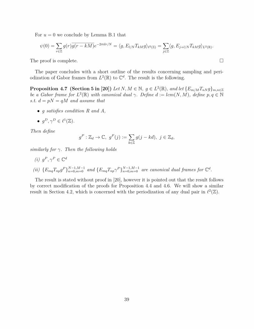
The paper concludes with a short outline of the results concerning sampling and peri-odization of Gabor frames from L2(R) to Cd. The result is the following.
Proposition 4.7 (Section 5 in [20]) Let N,M ∈ N, g ∈ L2(R), and let {Em/MTnNg}m,n∈Zbe a Gabor frame for L2(R) with canonical dual γ. Define d := lcm(N,M), define p, q ∈ Ns.t. d = pN = qM and assume that
• g satisfies condition R and A,
• gD, γD ∈ `1(Z).
Then definegP : Zd → C, gP (j) :=
∑k∈Z
g(j − kd), j ∈ Zd,
similarly for γ. Then the following holds
(i) gP , γP ∈ Cd
(ii) {EmqTnpgP}N−1,M−1n=0,m=0 and {EmqTnpγP}N−1,M−1
n=0,m=0 are canonical dual frames for Cd.
The result is stated without proof in [20], however it is pointed out that the result followsby correct modification of the proofs for Proposition 4.4 and 4.6. We will show a similarresult in Section 4.2, which is concerned with the periodization of any dual pair in `2(Z).
39
4.2 [34] – Gabor frames by sampling and periodizationWe now turn to the results due to Søndergaard. The results proven in [34] are very muchin the spirit of [20]. By use of sampling and so-called periodization operators it is shownhow one can go from a Gabor frame in one space to a Gabor frame in another space. Theresults include the transition of Gabor frames from
(i) L2(R) to L2([0, L]) by periodization,
(ii) L2(R) to `2(Z) by sampling,
(iii) L2([0, L]) to Cd by sampling,
(iv) `2(Z) to Cd by periodization,
(v) L2(R) to Cd by sampling and periodization.
Recall that the results in [20] state that sampling a canonical dual pair from L2(R) to `2(Z)preserves the canonical duality. This result is improved in [34] to hold for any dual pairin any of the transitions in (i)-(v) as described above. Furthermore, the results concerning(i),(ii),(iii) and (v) allow for sampling on lattices of the form αZ for specific α > 0, whichdepend on the translation parameter of the Gabor system in L2(R) or L2[0, L].
In Section 4.2.1, 4.2.2 and 4.2.3 we will go through the details of the transitions (ii),(iv)and (v) respectively. The main results are Theorem 4.16, 4.19 and 4.20. Especially Theorem4.20 is of importance, as we generalize this result in the new result shown in Section 5. InSection 4.3 Theorem 4.16 and 4.20 are applied to concrete examples.
The proofs in this section are of far less complexity compared to the proofs in Section 4.1.Before we turn to the details, we will introduce a new function space and two operators:In (ii) and (v) we again sample a function in L2(R) and therefore need to consider Lebesguepoints in order to make the sampling well defined, see Remark 4.2. A way around this issueis to consider window functions which lie in Feichtinger’s algebra S0(R).
Definition 4.8 (Feichtinger’s Algebra) A function g ∈ L2(R) belongs to Feichtinger’salgebra S0(R) if
‖g‖S0 =∫R×R|〈g, EωTxϕ〉| dxdω <∞,
where ϕ(t) = e−πt2 is the Gaussian function.
Remark 4.9 The space S0(R) is invariant under translation, modulation, dilation and theFourier transform. Furthermore S0(R) ⊆ Lp(R) for 1 ≤ p ≤ ∞ and all functions whichbelong to Feichtinger’s algebra are continuous and satisfy condition R and A for any trans-lation and modulation parameters. If g ∈ S0(R) generates a Gabor frame, then the canonicaldual also lies in S0(R). Consequently, to consider functions in S0(R) has many advantagesfor time-frequency analysis. Especially since g is continuous, the question concerning the
40
sampling of a function g ∈ S0(R) becomes obsolete. For more on S0(R) see [13, Chapter 3],[15, Chapter 12] and [22].
We will use the same notation as in [34] and therefore introduce the following two opera-tors.
Definition 4.10 Let α > 0. The sampling operator Sα is defined as
Definition 4.11 Let d ∈ N. The periodization operator Pd is defined as
Pd : `1(Z)→ Cd, (Pdf)(j) =∑k∈Z
f(j + kd), j ∈ Zd.
Remark 4.12 The fact that the sampling operator Sα is well defined from S0(R) into `1(Z)is a property of Feichtinger’s algebra, see [13, Lemma 3.2.11]. For Pd to be well defined, weneed to show that for all f ∈ `1(Z) and for all j = 0, 1, . . . , d− 1
In this section we generalize the results in [20] to hold for any dual pair. Also improvementsconcerning the sampling points are presented. There are two main results in this part:Theorem 4.14, concerning canonical dual pairs and Theorem 4.16, which is about samplingof any dual pair of Gabor frame generators.
By use of the sampling operator Sα defined above, we can summarize an implication ofJanssen’s results from Proposition 4.4 and 4.6 as follows:
Proposition 4.13 Let g ∈ S0(R), a,M ∈ N and {Em/MTnag}m,n∈Z be a Gabor frame forL2(R) with canonical dual γ. Then the following holds:
(i) {Em/MTnaS1g}M−1m=0,n∈Z is a Gabor frame for `2(Z) with the same frame bounds as
{Em/MTnag}m,n∈Z,
(ii) S1g and S1γ are a canonical dual pair.
41
Note that S1 indeed evaluates a function at the integers.The properties of the dilation operator (Proposition 2.6), allows for an easy generalization
of Proposition 4.13:
Theorem 4.14 (Theorem 2.4.1 in [34]) Let g ∈ S0(R), α, β > 0 and choose a,M ∈ Nsuch that αβ = a/M . If {EmβTnαg}m,n∈Z is a Gabor frame for L2(R) with canonical dualγ ∈ L2(R). Then the following holds:
(i) {Em/MTnaSα/ag}M−1m=0,n∈Z is a Gabor frame for `2(Z) with the same frame bounds as
{EmβTnαg}m,n∈Z,
(ii) Sα/ag and Sα/aγ are a canonical dual pair.
Proof. (i). By Proposition 2.6 is Da/α a unitary operator, hence Lemma 3.15 states that{EmβTnαg}m,n∈Z is a frame if and only if {Da/αEmβTnαg}m,n∈Z is a frame. The relationsbetween Dc, Eb and Ta from Proposition 2.6 imply that
Da/αEmβTnαg = Emβα/aTnαa/αDa/αg = Em/MTnaDa/αg.
This calculation shows that {Em/MTnaDa/αg}m,n∈Z is a frame with the same frame boundsas {EmβTnαg}m,n∈Z. By use of Proposition 4.13(i) we conclude that
(S1Da/αg)(j) =√α
ag(α
aj) = (Sα/ag)(j) (4.51)
is a Gabor frame generator for `2(Z) with a and 1/M as translation and modulation para-meters respectively.(ii). Let now γ denote the canonical dual generator of the Gabor frame {EmβTnαg}m,n∈Zand Sγ be the associated frame operator. We then have that
γ = Sγg =∑
m,n∈Z〈g, EmβTnαγ〉EmβTnαγ.
Applying Da/α to both sides and using the fact that Da/α is unitary, we find
Da/αγ =∑
m,n∈Z〈Da/αg,Da/αEmβTnαγ〉Da/αEmβTnαγ
=∑
m,n∈Z〈Da/αg, Em/MTnaDa/αγ〉Em/MTnaDa/αγ.
The right hand side is exactly SDa/αγDa/αg, where SDaαγ is the frame operator associatedwith Da/αγ and a and 1/M as translation and modulation parameter respectively. Weconclude that Da/αγ and Da/αg are a canonical dual pair with a and 1/M as translation andmodulation parameter. Proposition 4.13(ii) together with (4.51) then implies that Sα/aγ isthe canonical dual of Sα/ag. �
42
In Theorem 4.14 the generators are sampled at a lattice of the form αaZ. That is, the
generator is sampled equidistantly on intervals of the form [0, α[ over the real line. Thisis in contrast to the previous result by Janssen, where only the integers were allowed assampling-points.
We now turn to the results concerning sampling of any dual pair. We first need a lemma,which relates the Wexler-Raz relations for L2(R) and `2(Z).
Lemma 4.15 (Proposition 2.4.2 in [34]) Let α, β > 0 and a,M ∈ N be such thatαβ = a/M . With g, h ∈ S0(R) define
c(m,n) := 〈g, Em/αTn/βh〉L2(R) =∫Rg(x)h(x− n/β)e−2πimx/α dx, m, n ∈ Z.
For m = 0, 1, . . . , a− 1, n ∈ Z define
d(m,n) := 〈Sα/ag, Em/aTnMSα/ah〉`2(Z) = α
a
∑j∈Z
g(αaj)h(α
aj − nM α
a)e−2πimk/α.
Then d(m,n) =∑j∈Z
c(m− ja, n).
Proof. Define F (x) := g(x)h(x− n/β)e−2πimx/α. The Poisson summation formula (PSF)holds pointwise for g, h ∈ S0(R), see [15, eq. (1.37), Section 1.4] and [13, Corollary 3.2.9].We therefore have that∑
j∈Zc(m− ja, n) =
∑j∈Z
∫Rg(x)h(x− n/β)e−2πi(m−ja)x/α dx
=∑j∈Z
∫RF (x)e−2πixj(−a/α) dx
(PSF )= αa
∑j∈Z
F (αaj)
= αa
∑j∈Z
g(αaj)h(α
aj − nM α
a)e−2πimk/α = d(m,n).
In the last step we used that 1/β = Mα/a. �
We are now ready to show that we can sample any dual pair:
Theorem 4.16 (Proposition 2.4.3 in [34])Let g, h ∈ S0(R), α, β > 0 and a,M ∈ N besuch that αβ = a/M . If {EmβTnαg}m,n∈Z and {EmβTnαh}m,n∈Z form dual frames for L2(R),then {Em/MTnaSα/ag}M−1
m=0,n∈Z and {Em/MTnaSα/ah}M−1m=0,n∈Z form dual frames for `2(Z).
Proof. By use of the definitions in Lemma 4.15 and the Wexler-Raz relations in Theorem3.19, we know that
1αβc(m,n) = δmδn, m, n ∈ Z
43
and we need to show that
Mad(m,n) = δmδn, m = 0, 1, . . . , a− 1, n ∈ Z.
By the result stated in Lemma 4.15 we have the equality
Mad(m,n) =
∑j∈Z
1αβc(m− ja, n) =
∑j∈Z
δm−jaδn.
Since m = 0, 1, . . . , a− 1 is ∑j∈Z δm−ja = δm and we conclude that
Mad(m,n) = δmδn
as desired and the result follows. �
4.2.2 The transition from `2(Z) to Cd
In this section we will by means of periodization go from dual pairs in `2(Z) to dual pairs inCd. The proof if very similar to the previous case in Section 4.2.1 and we begin again witha lemma.
Lemma 4.17 (Proposition 2.4.11 in [34]) Let a, b, d,M,N ∈ N be such that Mb =Na = d. For g, h ∈ `1(Z) and m = 0, 1, . . . , a− 1, n ∈ Z define
c(m,n) := 〈g, Em/aTnMh〉`2(Z) =∑k∈Z
g(k)h(k − nM)e−2πimk/a.
For m = 0, 1, . . . ,M − 1, n = 0, 1, . . . , N − 1 define
By use of the relation between c(m,n) and d(m,n) in Lemma 4.17 we have that
MNdd(m,n) = M
a
∑j∈Z
c(m,n− jb) =∑j∈Z
δmδn−jb = δmδn.
In the last step we have used that n = 0, 1, . . . , b− 1. This completes the proof. �
4.2.3 The transition from L2(R) to Cd
Theorem 4.16 and 4.19 can easily be combined to the following result concerning the tran-sition from dual pairs in L2(R) to Cd.
45
Theorem 4.20 (Proposition 2.4.13 in [34]) Let g, h ∈ S0(R), α, β > 0 and a, b, d,M,N ∈N be chosen such that αβ = a/M = b/N and d = aN = bM . Then if {EmβTnαg}m,n∈Z and{EmβTnαh}m,n∈Z are dual frames for L2(R), then PdSα/ag and PdSα/ag form a dual pair forCd with translation and modulation parameter a and b respectively.
Without operator notation, the function PdSα/ag is given by
PdSα/ag(j) =√α
a
∑k∈Z
g(αaj − kNα), j ∈ Zd.
This concludes the discussion of the results from [34]. The proofs of transition (i) and(iii) (as described in the beginning of Section 4.2) can be shown by very similar ideas.
46
4.3 ExamplesIn the following we present a few concrete examples where we apply Proposition 4.4, 4.6and Theorem 4.20. The explicit dual pairs are taken from [2] and [4].
Figure 1: (Applying Proposition 4.4 and 4.6) On the left: the tight Gabor framegenerator g(x) = sin(2πx/3)χ[0,3] in blue; With α = 1 and β = 1/3 as translation andmodulation parameter respectively, the canonical dual is given by γ = 2
9g. γ is shown inred. On the right: g and γ are sampled at the integers and form a dual pair for `2(Z) witha = 1 and b = 1/3.
47
Figure 2: (Applying Theorem 4.20) On the left the tight Gabor frame generator g(x) =sin(2πx/3)χ[0,3] is shown in blue. For α = 1 and β = 1/3 as translation and modulationparameter respectively, it has the canonical dual γ = 2
9g. γ is shown in red. On the rightP60S1/10g and P60S1/10γ are shown. They form a dual pair for C60.
48
Figure 3: (Applying Theorem 4.20) The function g(x) = {x, if 0 ≤ x < 1; 2− x if 1 ≤x < 2; 0 otherwise} and h(x) = 1
5 [g(x) + 2g(x + 1)] are shown on the left in blue and redrespectively. g and h form a dual pair for α = 1 and β = 1/5 as translation and modulationparameter, see [2]. On the right P120S1/20g and P120S1/20h form dual a dual pair for C120
with a = 20 and b = 2 as translation and modulation parameter respectively.
49
5 New results on the sampling of Gabor framesWe now present new results on the sampling of dual Gabor pairs from L2(R) to Cd. In [20]the results concerning sampling of dual pairs are based on Lemma 3.18, whereas the centralresults needed in [34] are the Wexler-Raz relations from Theorem 3.19. In the following weshall use a third approach, namely the characterization equations for dual Gabor framespresented in Theorem 3.20. We show that this approach allows us to generalize the previousresult concerning sampling from L2(R) to Cd in Theorem 4.20. Specifically, we will showthat equidistant sampling points are not needed.
The section has the following structure: we begin by proving a lemma concerning sumswhich appear in the characterizing equations in Theorem 3.20. This is followed by themain result Theorem 5.2, which relies on certain technical conditions. As it turns out, thetechnical conditions are automatically satisfied if we restrict ourselves to sample functionsin Cc(R) or Feichtinger’s algebra S0(R). In Definition 5.4 we define a new (non-equidistant)sampling operator. This operator is well defined on Cc(R) and S0(R). Finally, the simpler,yet more elegant results compared to Theorem 3.20 are presented in Corollary 5.6 and 5.7.
In the following we shall need the periodization operator Pd for d ∈ N, defined as
Pd : `1(Z)→ Cd, (Pdf)(j) :=∑k∈Z
f(j + kd), j ∈ Zd.
That this operator is well defined is shown in Remark 4.12.We begin with a lemma concerning sums similar to those in the characterizing equations
of Theorem 3.20.
Lemma 5.1 Let g, h ∈ `1(Z) and choose the constants a, b, d,M,N ∈ N such that aN =bM = d. Assume that ∑
Proof. Straight forward calculations show that for all j ∈ ZdN−1∑k=0Pdg(j + nM + ak)Pdh(j + ak)
=N−1∑k=0
∑m∈Z
∑l∈Z
g(j + nM + ak + ld)h(j + ak +md)
(i)=N−1∑k=0
∑m∈Z
∑l∈Z
g(j + nM + ak + [l +m]d)h(j + ak +md)
=N−1∑k=0
∑m∈Z
∑l∈Z
g(j + nM + a[k +mN ] + lbM)h(j + a[k +mN ])
(ii)=∑k∈Z
∑l∈Z
g(j + nM + ak + lbM)h(j + ak)
=∑k∈Z
∑l∈Z
g(j + (n+ lb)M + ak)h(j + ak) (iii)=∑l∈Z
δn+lb.
(i). This equality holds since m+ l runs through all the integers.(ii). Since k = 0, 1, . . . , N − 1 and m ∈ Z will k +mN run through all integers.(iii). This equality holds is by assumption.Since l ∈ Z, b ∈ N and n = 0, 1, . . . , b − 1 is δn+lb = 0 if and only if l = b = 0. Therefore is∑l∈Z δn+lb = δn. This completes the proof. �
We are now ready for the main result.
Theorem 5.2 Let g, h ∈ L2(R) be dual Gabor generators for L2(R) with translation para-meter α > 0 and modulation parameter β > 0. Choose a, b, d, s,M,N ∈ N such that
αβ
s= a
M= b
Nand d = Na = Mb.
Let {xj}a−1j=0 ⊂ [0, α[ be a finite sequence in the interval [0, α[ such that the characterizing
equations for dual Gabor frames in L2(R)∑k∈Z
g(x− n/β − kα)h(x− kα) = β δn, ∀n ∈ Z (5.2)
are satisfied pointwise for all {xj}a−1j=0 . Then define
Multiplying on both sides by 1/M results in the characterizing equations for
{EmbTna(Mβ)−1/2Pdg}M−1,N−1m=0,n=0 and {EmbTna(Mβ)−1/2Pdh}M−1,N−1
m=0,n=0
to form dual Gabor frames for Cd, see Theorem 3.20(ii). The proof is complete. �
Remark 5.3 (i) The essential part in the proof is the requirement that the characterizingequations for dual Gabor generators are satisfied pointwise for the chosen {xj}a−1
j=0 . Comparethis with Theorem 3.20(i), where the characterizing equations only need to be satisfieda.e. x ∈ [0, α].(ii). In practice, explicit dual pairs will usually be defined as piecewise continuous functions,
52
e.g., piecewise polynomials. Hence, the task to find {xj}a−1j=0 ⊂ [0, α[ where the characterizing
equations are satisfied pointwise is trivial. Especially if g and h are continuous functions,then 3.20(i) is satisfied for all x ∈ [0, α[.(iii) Remarkably, the order of the {xj}a−1
j=0 is irrelevant. This fact allows for the constructionof dual pairs of generators in Cd which can not be covered by Theorem 4.20.(iv) The requirement that g, h ∈ `1(Z) is necessary for Pdg and Pdh to be well defined.Note that if the generators g and h have compact support, then trivially g, h ∈ `1(Z).
From Remark 5.3(ii) and (iv) we can immediately formulate a simplified version of The-orem 5.2. Before we state the result, we ease notation by introducing a new samplingoperator.
Definition 5.4 Let α > 0, a ∈ N. Take {xj}a−1j=0 ⊂ [0, α[ to be a finite sequence in the
Let x := {xj}j∈Z. Then for a function f : R→ C we define the sequence Sxa,αf as
Sxa,αf(j) := f(xj), j ∈ Z.
Proposition 5.5 The sampling operator Sxa,α is well defined
(i) as a mapping from Cc(R) to `1(Z) ;
(ii) as a mapping from S0(R) to `1(Z) .
Proof. (i). If f ∈ Cc(R) then xj ∈ supp f only for a finite number of j ∈ Z. Hence, thereexists an N ∈ N such that∑
j∈Z|Sxa,αf(j)| =
∑|j|≤N
|Sxa,αf(j)| ≤ (2N + 1) max
x∈R|f(x)| <∞.
(ii). To show that Sxa,α is well defined on S0(R), observe that due to [13, Lemma 3.2.11] the
operator
Sα : S0(R)→ `1(Z), Sαf(j) := f(αj), j ∈ Z, (5.3)
is well defined (compare this with Definition 4.10 and Remark 4.12). Using the operator Sα,we have that for any f ∈ S0(R)
∑j∈Z|Sxa,αf(j)| =
a−1∑k=0
∑j∈Z|SαT−xkf(j)|. (5.4)
53
Define fk := T−xkf for k = 0, 1, . . . , a− 1. Since S0(R) is invariant under translation, all fkbelong to S0(R). We therefore have that {Sαfk(j)}j∈Z ∈ `1(Z). Continuing the calculationin (5.4), we conclude that
∑j∈Z|Sxa,αf(j)| =
a−1∑k=0
∑j∈Z|Sαfk(j)|︸ ︷︷ ︸<∞
<∞.
�
Note that applying the operator Sxa,α to a function g : R→ C exactly yields the sequence
g as in Theorem 5.2. The following two corollaries now follow from Remark 5.3.
Corollary 5.6 Let g, h ∈ Cc(R) be dual Gabor generators for L2(R) with translation pa-rameter α > 0 and modulation parameter β > 0. Choose a, b, d, s,M,N ∈ N such that
αβ
s= a
M= b
Nand d = Na = Mb.
Take Sxa,α as in Definition 5.4. Then
{EmbTna(Mβ)−1/2PdSxa,αg}
M−1,N−1m=0,n=0 and {EmbTna(Mβ)−1/2PdSx
a,αh}M−1,N−1m=0,n=0
form dual Gabor frames for Cd.
Corollary 5.7 Let g, h ∈ S0(R) be dual Gabor generators for L2(R) with translation pa-rameter α > 0 and modulation parameter β > 0. Choose a, b, d, s,M,N ∈ N such that
αβ
s= a
M= b
Nand d = Na = Mb.
Take Sxa,α as in Definition 5.4. Then
{EmbTna(Mβ)−1/2PdSxa,αg}
M−1,N−1m=0,n=0 and {EmbTna(Mβ)−1/2PdSx
a,αh}M−1,N−1m=0,n=0
form dual Gabor frames for Cd.
Remark 5.8 If s = 1 and we take x = {0, α/a, 2α/a, . . . , (a− 1)α/a} then is
(Mβ)−1/2PdSxa,αg(j) =
√α
a
∑k∈Z
g(αaj − kNα) = PdSα/ag(j). (5.5)
Here Sα/a is the sampling operator from Definition 4.10 used in [34]. The right hand side of(5.5) is exactly what we find in Theorem 4.20.
54
5.1 ExamplesIn the following Theorem 5.2 is applied to a few concrete examples of dual pairs of Gaborframe generators. Note the freedom in choosing the sampling sequence x as noted in Remark5.3(iii). The dual pairs are taken from [4].
Figure 4: On the left is the tight Gabor frame generator g(x) = sin(2πx/3)χ[0,3] (blue). Forα = 1 and β = 1/3 the canonical dual is given by γ = 2
9g, which is shown in red. On theright g and γ are sampled with x = {0, 0.1, 0.1, 0.1, 0.3, 0.3, 0.3, 0.3, 0.3, 0.3} and form a dualpair for Cd with d = 60, a = 10, b = 2,M = 30 and N = 6.
55
Figure 5: On the left the tight Gabor frame generator g(x) = sin(2πx/3)χ[0,3] is shown inblue. For α = 1 and β = 1/3 the canonical dual is given by γ = 2
9g, which is shown in red.On the right g and γ are sampled with x = {0.9, 0.1, 0.8, 0.2, 0.7, 0.3, 0.6, 0.4, 0.5, 0.5} andform a dual pair for Cd with d = 60, a = 10, b = 2,M = 30 and N = 6.
56
Figure 6: On the left the tight Gabor frame generator g(x) = sin(2πx/3)χ[0,3] is shown inblue. For α = 1 and β = 1/3 the canonical dual is given by γ = 2
9g, which is shown in red.On the right g and γ are sampled with x = {0.1, 0.1, 0.1, 0.1, 0.1, 0.1, 0.1, 0.1, 0.1, 0.1} andform a dual pair for Cd with d = 60, a = 10, b = 2,M = 30 and N = 6.
57
Figure 7: On the left is the Gabor frame generator g(x) = sin3(πx/3)χ[0,3] is shown in blue.For α = 1 and β = 1/5 a dual is given by h(x) = 64
405 [g(x) + g(x + 1) − g(x + 2)], which isshown in red. On the right g and h are sampled with x = {0, 0.05, 0.1, 0.15, . . . , 0.55} andform a dual pair for Cd with d = 120, a = 12, b = 2,M = 60 and N = 10.
58
6 Sampling of other systemsIn the following we talk about sampling and periodization of shift-invariant and waveletframes. Both systems exist in L2(R) and are defined by use of the translation operator Taand dilation operator Dc, see Definitions 2.1 and 2.5 respectively.
The literature on wavelets is very extensive, see for example [11], [16] and [36]. Forinformation on shift-invariant systems we refer to [3] and [32]. In the following we will byno means introduce the theory of these systems in detail and only state results which areneeded.
In the case of shift-invariant systems we formulate a preliminary result on sampling dualshift-invariant frames from L2(R) to Cd. The theory of wavelet systems is more challengingdue to the lack of a dilation operator on Cd. However, we define both dilation and waveletsystems for Cd such that the resulting characterizing equations for dual wavelet frames ofL2(R) and Cd have striking similarities!
6.1 Sampling of shift-invariant framesIn this section we introduce shift-invariant systems in L2(R) and Cd. The main result willbe a sampling-theorem for shift-invariant systems from L2(R) to Cd, which is very similarto Theorem 5.2.
We define shift-invariant systems as follows:
Definition 6.1 (Shift-invariant system)
(i) Let A be a countable set and {gm}m∈A be a collection of functions in L2(R). Theshift-invariant system generated by {gm}m∈A and shift parameter a > 0 is the familyof functions given by
{Tnagm}n∈Z,m∈A = {gm( · − na)}n∈Z,m∈A.
(ii) Let A be a finite set and {gm}m∈A be a collection of functions in Cd. Choose theconstants a, d,N ∈ N such that aN = d. The shift-invariant system generated by{gm}m∈A and shift parameter a is the family of functions given by
{Tnagm}N−1n=0,m∈A = {gm(· − na)}N−1
n=0,m∈A.
Remark 6.2 A shift-invariant system in Cd could in principal be generated by an infinitecountable family {gm}. However, since Cd is finite dimensional, the requirement for A to befinite seems adequate.
For our purposes we only need the following result:
Theorem 6.3 Concerning dual shift-invariant system the following holds:
59
(i) Let {gm}m∈A, {hm}m∈A ∈ L2(R) and a > 0 be given. Two Bessel sequences {Tnagm}n∈Z,m∈Aand {Tnahm}n∈Z,m∈A form dual frames for L2(R) if and only if∑
m∈Agm(x+ k/a) hm(x) = aδk, a.e. x ∈ R, ∀k ∈ Z.
(ii) Let {gm}m∈A, {hm}m∈A ∈ Cd be given and choose a, d,N ∈ N such that d = aN . TwoBessel sequences {Tnagm}N−1
n=0,m∈A and {Tnahm}N−1n=0,m∈A form dual frames for Cd if and
The result in (i) is due to Ron and Shen, [32]. The proof of (ii) is given in Appendix A. Wecan now formulate the following sampling theorem:
Theorem 6.4 Let A be a finite set, {gm}A and {hm}m∈A be dual shift invariant systemsfor L2(R) with shift parameter α > 0 and choose a, d,N ∈ N such that aN = d. Let {xj}d−1
j=0be a sequence in R, for which the following holds:
(i) the characterizing equations in Theorem 6.3(i) are satisfied pointwise for all xj.
(ii) for k = 1, 2, . . . , a− 1 and j ∈ Zd will xj+kN − xj ∈ kαZ\{0}.
Then for j ∈ Zd define the finite sequences
gm(j) := (αN)−1/2gm(xj), hm(j) := (αN)−1/2hm(xj).
If gm, hm ∈ Cd, then {Tnag,}N−1n=0,m∈A and {Tnah,}N−1
n=0,m∈A are dual shift invariant systems forCd.
Proof. By definition of gm and hm, we have that for any j ∈ Zd and k = 0, 1, . . . , a− 1
∑m∈A
gm(j + kN) hm(j) = 1αN
∑m∈A
gm(xj+kN) hm(xj). (6.1)
Requirement (ii) in the definition of the sequence {xj}d−1j=0 implies that there exists a non-
zero integer s ∈ Z \ {0} such that xj+kN = xj + ks/α. Using this on the right hand side in(6.1), we find that
∑m∈A
gm(j + kN) hm(j) = 1αN
∑m∈A
gm(xj + ks/α) hm(xj). (6.2)
By requirement (i) we know that∑m∈A
gm(xj + ks/α) hm(xj) = α δks = α δk.
60
The last equality is due to the fact that s is non-zero. From (6.2) then follows that
∑m∈A
gm(j + kN) hm(j) = 1Nδk.
�
Remark 6.5 For the Theorem to hold, we need the set A to be finite. Currently there isno result on how to generate a pair of dual shift-invariant systems {gm}m∈A and {hm}m∈Afor Cd from a dual shift-invariant system {gm}m∈A and {hm}m∈A in L2(R), where A is finiteand A is an infinite countable set.
6.2 Sampling of wavelet framesWavelet systems in L2(R) are defined by using the translation and dilation operator.
Recall from Definition 2.5 and Proposition 2.6 that the dilation operator Dc for c > 0 isdefined as
Dc : L2(R)→ L2(R), (Dcf)(x) := c−1/2f(x/c), x ∈ R. (6.3)
Moreover, it has the following properties:
DcTa = TacDc, (6.4)
Dc = F−1D1/cF . (6.5)
Wavelet systems in L2(R) are defined as follows:
Definition 6.6 (Wavelet system) Let ψ ∈ L2(R) and a > 1, b > 0. The wavelet systemgenerated by ψ with scaling paramater a and translation parameter b is the system
{DajTnbψ}j,n∈Z = {a−j/2ψ( · /aj − nb)}j,n∈Z .
Naturally, if a wavelet system is a frame, then we call it a wavelet frame.To give an analog definition in Cd is a major challenge, because no dilation operator on
Cd exists.
Remark 6.7 This does not mean that no wavelet theory in Cd exists. In fact, there isthe so-called discrete wavelet transform and wavelets are heavily used in, e.g., image andsignal processing. However, this theory does not rely on the definition of an explicit dilationoperator nor does it provide a direct analog to wavelet systems as in Definition 6.6.
61
In order to apply the previous approach shown in the Gabor and shift-invariant case,we need similar characterizing equations for dual wavelet systems in L2(R) and Cd. In thefollowing we define certain operators and wavelet-like systems in Cd for which we indeedshow characterizing equations similar to the characterizing equations for dual wavelet framesin L2(R).
We begin with a definition of pairs of dilation-like operators on Cd.
Definition 6.8 (Pairs of dilation-like operators) For c ∈ N, let Dc and D1/c be linearmappings from Cd to Cd. We say that Dc and D1/c are a pair of dilation-like operators, iffor all f ∈ Cd they satisfy
(i) D1f = D1/1f = f ;
(ii) Dcf = F−1D1/cF f ;
(iii) DcTaf = TacDcf .
The properties of dilation-like operators and the dilation operator on L2(R) are verysimilar, see (6.4) and (6.5).
The existence of such a pair is established by the following Proposition.
Proposition 6.9 Let c, d ∈ N and c be a divisor of d. Define the operator
D1/c : Cd → Cd, (D1/cf)(x) :=
f(cx) c|x| ≤ d/20 otherwise
, for x ∈ {d−d2e, . . . , b−
d2c+ d}.
Furthermore, define Dc := F−1D1/cF . Then Dc and D1/c are a pair of wavelet-like operatorson Cd.
Proof. We need to verify (i)-(iii) in Definition 6.8.(i) If c = 1, then is (D1/1f)(x) = f(x) and for D1 we thus have D1 = F−1IF = I.(ii) This holds by definition of Dc.(iii) Note that
(D1/cEbf)(x) =
(Ebf)(cx) c|x| ≤ d/20 otherwise
=
e2πibcx/df(cx) c|x| ≤ d/20 otherwise
= EbcD1/cf(x).
By use of this relation and Proposition 2.4, we find that
With a pair of dilation-like operators in hand we define a wavelet-like system in Cd.
62
Definition 6.10 (Wavelet-like systems) Let ψ ∈ Cd, a, b ∈ N, a > 1 and J ⊂ N befinite. For each j ∈ J take Nj ∈ d
ajbN. The wavelet-like system generated by ψ under
the pair of dilation-like operators Dc and D1/c with scaling parameter a and translationparameter b is the family of functions in Cd of the form
{DajTnbψ}Nj−1n=0, j∈J .
Remark 6.11 (i) If Nj /∈ dajb
N then the characterization result in Theorem 6.12(ii) for dualwavelet-like systems does not hold.(ii) Note that depending on the definition of the pair of dilation-like operators Dc and D1/c,only certain values of a, j ∈ N may be allowed.
If a wavelet-like system is a frame we call it a wavelet-like frame. For dual wavelet andwavelet-like frames we have the following characterization.
Theorem 6.12 Concerning dual wavelet(-like) systems the following holds.
(i) Let ψ, φ ∈ L2(R) and a > 1, b > 0. Two Bessel sequences {DajTnbψ}j,n∈Z and{DajTnbφ}j,n∈Z are dual wavelet frames for L2(R) if and only if for all α ∈ 1
bZ
∑j∈Z:α∈ajZ
aj
bD1/aj ψ(x+ α)D1/aj φ(x) = δα a.e. x ∈ R.
(ii) Let ψ, φ ∈ Cd, a, b ∈ N, a > 1 and Dc, D1/c be a pair of dilation-like operators. Twowavelet-like systems {DajTnbψ}
Nj−1n=0, j∈J and {DajTnbφ}
Nj−1n=0, j∈J are dual frames for Cd
if and only if for all α ∈ Zd∑j∈J :α∈ d
ajbZ
Nj D1/aj ψ(x+ α)D1/aj φ(x) = δα ∀x ∈ Zd.
For the proof of (i) see [1] or [9]. The proof of (ii) is given in Appendix A.The similarity between the two characterizations indicates that a sampling result similar
to Theorem 5.2 for Gabor systems and Theorem 6.4 for shift-invariant systems may indeedbe possible for wavelet and wavelet-like systems.
63
7 Explicit constructions of dual Gabor generators inL2(R)
In this section we show new results on the explicit construction of dual Gabor generatorsin L2(R). The results are based on [2] and [7], which utilises the characterizing equationsfor dual Gabor generators, see Theorem 3.20. The standard assumption is the so-calledpartition of unity condition. We show more results under this assumption and introduce anew and similar notion of the “alternating” partition of unity condition.
In Section 7.1 we go through the known results of [2] and [7], which we generalize inSection 7.2. In Section 7.3 we show the result concerning the new “alternating” partition ofunity condition.
Remark 7.1 In the literature many explicit constructions of dual Gabor generators havefocused on the characterizing equations for dual Gabor generators in L2(R). Since thecharacterizing equations are similar for L2(R) and Cd, it is almost certain that the ideas ofthe explicit constructions in a much similar form must apply to explicit constructions in Cd.
7.1 Results from [2] and [7]In the construction of explicit dual frames {EmbTnag}m,n∈Z and {EmbTnah}m,n∈Z for L2(R)Theorem 3.20(i) is the central result. It states that two Bessel sequences {EmbTnag}m,n∈Zand {EmbTnah}m,n∈Z form dual frames if and only if∑
k∈Zg(x− n/b− ka)h(x− ka) = b δn, a.e. x ∈ [0, a], ∀n ∈ Z. (7.1)
Remark 7.2 (i) It can be shown that if f ∈ L2(R) is bounded and has compact support,then the Gabor system {EmbTnag}m,n∈Z is a Bessel sequence for any translation and modu-lation parameters a, b > 0. In the following we always consider such functions and we aretherefore only concerned in solving equation (7.1).(ii) For n = 0 equation (7.1) becomes (up to scaling) a partition of unity condition on thetranslates of the function gh:∑
k∈Zg(x− ka)h(x− ka) = b a.e. x ∈ [0, a]. (7.2)
A result due to Christensen in [2] shows that if g has compact support and satisfies thepartition of unity condition for its integer translates (eq. (7.3)), then there is an easy wayto construct an explicit dual h such that the characterization of dual Gabor generators issatisfied. The result is formulated in Theorem 7.3.
64
Theorem 7.3 Let N ∈ N. Let g ∈ L2(R) be a real valued bounded function with supp g ⊆[0, N ], for which ∑
n∈Zg(x− n) = 1. (7.3)
Let b ∈]0, 1/(2N − 1)]. Then the function g and the function h defined by
h(x) = b(g(x) + 2
N−1∑n=1
g(x+ n))
(7.4)
generate dual frames {EmbTng}m,n∈Z and {EmbTnh}m,n∈Z for L2(R).
Proof. The property that both {EmbTng}m,n∈Z and {EmbTnh}m,n∈Z are Bessel sequencesfollows from the fact that both functions have compact support and are bounded, see Remark7.2(i). By equation (7.1) we therefore only need to show that∑
Remark 7.4 Note that the idea of the proof is the assumption 1 = ∑N−1k=0 g(x + k), and
hence 1 = [∑N−1k=0 g(x + k)]2. In Theorem 7.7 we show new results with the starting point
being 1 = [∑N−1k=0 g(x+ k)]p for any p ∈ N, p > 1.
The result in Theorem 7.3 constructs a dual h as a one-sided sum of translations of g. In[7] the result of Theorem 7.3 has successfully been extended to also cover duals h which aregiven by a two-sided sum of translates of g. The result is as follows:
Theorem 7.5 Let N ∈ N. Let g ∈ L2(R) be a real-valued bounded function with supp ⊂[0, N ], for which ∑
n∈Zg(x− n) = 1.
Let b ∈]0, 1/(2N − 1)]. Consider any scalar sequence {an}N−1n=−N+1 for which
a0 = b and an + a−n = 2b, n = 1, 2, 3 . . . , N − 1,
and define h ∈ L2(R) by
h(x) =N−1∑
n=−N+1ang(x+ n).
Then g and h generate dual frames {EmnTng}m,n∈Z and {EmbTnh}m,n∈Z for L2(R).
The special choice an = b for all n = −N + 1, . . . , N − 1 yields the following corollary.
Corollary 7.6 Under the assumptions in the previous theorem, the function
h(x) = bN−1∑
n=−N+1g(x+ n)
generates a dual of {EmbTng}m,n∈Z. The function h satisfies that h = b on the support of g.Furthermore, if g is symmetric, then h is symmetric.
In Proposition 7.12 we generalize Corollary 7.6 by a similar idea as the one expressed inRemark 7.4.
66
7.2 New explicit constructions of dual Gabor generators for L2(R)We shall now generalize the result from Theorem 7.3 in the sense that under the sameconditions we will construct a family of duals hp which includes the result from Theorem7.3.
Theorem 7.7 Let N ∈ N. Let g ∈ L2(R) be a real-valued bounded function with supp g ⊆[0, N ], for which ∑
k∈Zg(x+ k) = 1. (7.7)
Let b ∈]0, 1/(2N − 1)] and fix p ∈ N, p ≥ 2. Then the function g and the function hp definedby
hp(x) = b∑
k0+k1+···+kN−1=pki∈N0,k0>0
(p
k
)g(x)k0−1
N−1∏j=1
g(x+ j)kj (7.8)
generate dual frames {EmbTng}m,n∈Z and {EmbTnhp}m,n∈Z for L2(R).
Proof. Note that the support of hp is the same as for h in Theorem 7.3. We can thereforefollow the same steps as in the proof of Theorem 7.3 and the only thing we need to show isthat
b =∑k∈Z
g(x− k)h(x− k) =N−1∑k=0
g(x+ k)h(x+ k) a.e. x ∈ [0, 1]. (7.9)
Due to the compact support of g and (7.15), we have that for x ∈ [0, 1]
1 =∑k∈Z
g(x+ k) =N−1∑k=0
g(x+ k) =(N−1∑k=0
g(x+ k))p.
By use of Theorem C.2 this becomes
1 =∑
k0+k1+···+kN−1=pki∈N0
(p
k
)N−1∏j=0
g(x+ j)kj . (7.10)
The set over which the summation is taken can be identified as Γp(I), where I = {0, 1, . . . , N−1}. By Lemma C.3 the set Γp(I) can be partitioned into N disjoint sets Γp,i(I), i ∈ I definedby
Γn,i(I) := { (kα)α∈I ∈ Γn(I) | ki > 0 and kl = 0 for l < i}.
That isΓp(I) =
N−1⋃i=0
Γp,i(I).
67
Using this partition on the right hand side in (7.10) yields
1 =N−1∑i=0
∑(k0,k1,...,kN−1)∈Γp,i(I)
(p
k
)N−1∏j=0
g(x+ j)kj .
Recall that by the definition of Γp,i(I) is kj = 0 for j < i, so we may in fact change thelimits in the product, so that
1 =N−1∑i=0
∑(k0,k1,...,kN−1)∈Γp,i(I)
(p
k
)N−1∏j=i
g(x+ j)kj
=N−1∑i=0
∑(k0,k1,...,kN−1)∈Γp,i(I)
(p
k
)g(x+ i)ki
N−1∏j=i+1
g(x+ j)kj .
Note that ki > 0 for (k0, k1, . . . , kN−1) ∈ Γp,i(I), thus we have
1 =N−1∑i=0
g(x+ i) ∑
(k0,k1,...,kN−1)∈Γp,i
(p
k
)g(x+ i)ki−1
N−1∏j=i+1
g(x+ j)kj. (7.11)
The term in the square brackets depends on the index i. Let us therefore denote the termin the square brackets by a function ϕi evaluated at x. That is,
ϕi(x) :=∑
(k0,k1,...,kN−1)∈Γp,i(I)
(p
k
)g(x+ i)ki−1
N−1∏j=i+1
g(x+ j)kj
The goal is now to identify ϕi(x) as hp(x+ i)/b. By changing the limits in the product andwriting out the definition of Γp,i(I), we get
ϕi(x) =∑
k0+k1+···+kN−1=pkn∈N0,ki>0,kl=0 for l<i
(p
k
)g(x+ i)ki−1
N−1−i∏j=1
g(x+ j + i)kj+i .
Due to the compact support of g and the fact that x ∈ [0, 1] we can change the set overwhich the sum is taken into the following.
ϕi(x) =∑
k0+k1+···+kN−1=pkn∈N0,k0>0
(p
k
)g(x+ i)k0−1
N−1−i∏j=1
g(x+ j + i)kj .
And again due to the compact support of g we can change the limits in the product to theones we see in the definition of h in (7.8).
ϕi(x) =∑
k0+k1+···+kN−1=pkn∈N0,k0>0
(p
k
)g(x+ i)k0−1
N−1∏j=1
g(x+ j + i)kj = hp(x+ i)/b.
68
Combining this with (7.11) yields b =N−1∑i=0
g(x+ i)hp(x+ i), as desired. �
Remark 7.8 (i) Theorem 7.7 with the choice p = 2 yields the results in Theorem 7.3.(ii) The set over which the summation in (7.8) is taken is rather complicated. This makes theactual computation of the dual generator hp difficult. This issue is resolved in Proposition7.11, where a much simpler expression for hp is presented.(iii) Note that the complexity of the expression for hp grows as p and the support of gincrease.
The following is an example of a pair of dual generators g and h4 given by Theorem 7.7,where we verify that (7.9) is satisfied.
Example 7.9 Consider the B-spline N4 given by
N4(x) =
16x
3 x ∈ [0, 1[,16 + 1
2x+ 12x
2 − 12x
3 x ∈ [1, 2[,23 − x
2 + 12x
3 x ∈ [2, 3[,16 − 12x+ 1
2x2 − 1
6x3 x ∈ [3, 4[,
0 x /∈ [0, 4[.
(7.12)
It is well known that the B-splines, and in particular N4 satisfy the partition of unitycondition (7.15). Moreover, N4 is real-valued, bounded and suppN4 = [0, 4]. That is, N4satisfies all conditions needed to apply Theorem 7.7. We will consider the dual h4, whichsatisfies
As mentioned before, the calculation of the dual generator h in Theorem 7.7 is cumber-some. The following result resolves this problem.
71
Proposition 7.11 Consider g and hp as in Theorem 7.7. Then
hp(x) =
b
g(x)
[(N−1∑j=0
g(x+ j))p−(N−1∑
j=1g(x+ j)
)p]a.e. x ∈ supp g,
b p(N−1∑
j=1g(x+ j)
)p−1a.e. x /∈ supp g.
(7.13)
Proof. Consider first the situation where x ∈ supp g. In that case g(x) 6= 0 almosteverywhere. Multiplying (7.8) with g(x) yields
g(x)hp(x)
= b∑
k0+k1+···+kN−1=pki∈N0,k0>0
(p
k
)N−1∏j=0
g(x+ j)kj
= b
∑k0+k1+···+kN−1=p
ki∈N0
(p
k
)N−1∏j=0
g(x+ j)kj −∑
k0+k1+···+kN−1=pki∈N0,k0=0
(p
k
)N−1∏j=0
g(x+ j)kj
= b
∑k0+k1+···+kN−1=p
ki∈N0
(p
k
)N−1∏j=0
g(x+ j)kj −∑
k1+k2+···+kN−1=pki∈N0
(p
k
)N−1∏j=1
g(x+ j)kj
Using the Multinomial formula on the two expressions on the right hand side we have that
g(x)hp(x) = b[(N−1∑
j=0g(x+ j)
)p−(N−1∑
j=1g(x+ j)
)p](7.14)
Since g(x) 6= 0 almost everywhere, (7.14) yields
hp(x) = b
g(x)
[(N−1∑j=0
g(x+ j))p−(N−1∑
j=1g(x+ j)
)p].
Assume now that x /∈ supp g. Then g(x) = 0 a.e. and by (7.8)
hp(x) = b∑
k0+k1+···+kN−1=pki∈N0,k0>0
p!k0!k1! · · · kN−1! g(x)︸ ︷︷ ︸
=0 a.e.
k0−1N−1∏j=1
g(x+ j)kj .
Only for k0 = 1 will the summands be non-zero, since then 00 = 1. Thus
hp(x) = b∑
k1+···+kN−1=p−1ki∈N0,k0=1
p(p− 1)!k1! · · · kN−1!
N−1∏j=1
g(x+ j)kj
72
By the Multinomial formula we then have that
hp(x) = b p(N−1∑
j=1g(x+ j)
)p−1a.e. x /∈ supp g.
�
This result allows us to compute the duals proposed in Theorem 7.7 in an easy way.It is well known that the B-splines Nm,m ∈ N satisfy the partition of unity condition.
Constructions of the dual generator h for generators g = N2 and g = N4 can be seen inFigure 9 and 10 respectively. In each figure we let p ∈ {2, 3, 4, 8}.
Figure 9: Dual generators hp for g = N2 with p = 2, 3, 4, 8.
73
Figure 10: Dual generators hp for g = N4 with p = 2, 3, 4, 8.
As it turns out, the result in Theorem 7.7 can not easily be extended to include duals ofthe form similar to those in Theorem 7.5. However, for the new constructions in Theorem7.7 we can easily show a result similar to that of Corollary 7.6.
Proposition 7.12 Let N ∈ N. Let g ∈ L2(R) be a real-valued bounded function withsupp g ⊆ [0, N ], for which ∑
k∈Zg(x+ k) = 1. (7.15)
Let b ∈]0, 1/(2N − 1)] and fix p ∈ N. Then the function
hp(x) = b( N−1∑n=−N+1
g(x+ n))p
generates a dual Gabor frame for {EmbTng}m,n∈Z. The function hp satisfies that hp = b onthe support of g. Furthermore, if g is symmetric, then hp is symmetric.
Proof. The property that both {EmbTng}m,n∈Z and {EmbTnhp}m,n∈Z are Bessel sequencesfollows from the fact that both functions have compact support and are bounded, see Remark7.2(i). By equation (7.1) we therefore only need to show that∑
Remark 7.14 Preliminary observations indicate that functions satisfying the “alternating”partition of unity condition (7.19) can not be continuous. This is certainly not the case forfunctions satisfying the usual partition of unity condition.
76
A Duality conditions for frames in Cd
In the following we present the proofs of the characterizing equations for dual Gabor, shift-invariant and wavelet-like frames in Cd. The results respectively appear in Theorem 3.20,6.3 and 6.12.
We begin by stating an essential lemma.
Lemma A.1 Let N ∈ N, then
N−1∑n=0
e2πinx/N =
N if x ∈ NZ,0 if x ∈ Z\NZ.
Proof. If x ∈ NZ, then an element k ∈ Z exists such that x = kN . We therefore havethat
For N = 1 is Z \ NZ = ∅ and there is nothing to prove. Let therefore N > 1 andx ∈ Z \NZ. Then the elements k ∈ Z and j ∈ {1, 2, . . . , N − 1} exist such that x = kN + j.With that is
Since j ∈ {1, 2, . . . , N − 1} is z := e2πij/N 6= 1 and we therefore have that
N−1∑n=0
e2πinx/N =N−1∑n=0
(e2πij/N)n =N−1∑n=0
zn = zN − 1z − 1 = (e2πij/N)N − 1
e2πij/N − 1 = e2πij − 1e2πij/N − 1 = 0.
�
The lemma in fact follows from a more general result, see [17, 23.19] and [1, Lemma 3.6],which may be used to state Theorems 3.20, 6.3 and 6.12 in higher dimensions.
77
A.1 Gabor framesTheorem A.2 Let g, h ∈ Cd and a, b, d,M,N ∈ N be chosen such that aN = bM = d.Then {EmbTnag}N−1,M−1
n=0,m=0 and {EmbTnah}N−1,M−1n=0,m=0 are dual Gabor frames for Cd if and only
ifN−1∑k=0
g(x− nM − ak)h(x− ak) = 1Mδn,0
holds for all x ∈ {0, 1, . . . , a− 1} and n ∈ {0, 1, . . . , b− 1}.
Proof. If {EmbTnag}N−1,M−1n=0,m=0 and {EmbTnah}N−1,M−1
n=0,m=0 are dual Gabor frames for Cd, then
f =N−1∑n=0
M−1∑m=0〈f, EmbTnag〉EmbTnah, ∀f ∈ Cd.
This equation is satisfied pointwise for each x ∈ Zd, hence for all f ∈ Cd
Note here, that above equality has to hold pointwise and for all f ∈ Cd. For (A.1) to hold,it is therefore necessary and sufficient that the expression in the square bracket is equal toone exactly when ξ = x and zero otherwise. We thus have that
f =N−1∑n=0
M−1∑m=0〈fEmbTnag〉EmbTnah, ∀f ∈ Cd
⇔N−1∑n=0
g(ξ − na)h(x− na)M−1∑m=0
e2πi(x−ξ)mb/d =
1 x = ξ,
0 x 6= ξ,∀x, ξ ∈ Zd. (A.2)
By use of Lemma A.1 we find that
N−1∑m=0
e2πim(x−ξ)mb/d =N−1∑m=0
e2πim(x−ξ)m/M =
M x− ξ ∈MZ,0 x− ξ ∈ Z \MZ.
We now have three different cases:
78
(i) If x = ξ, then (x− ξ) ∈MZ and (A.2) equals
N−1∑n=0
g(x− na)h(x− na) = 1M, ∀x ∈ {0, 1, . . . , a− 1}
Here we have also used the fact that the term on the left hand side of (A.2) is a-periodic.
(ii) If x 6= ξ and (x − ξ) ∈ MZ, then there exists k ∈ Z s.t. ξ = x − kM . Specifically,since bM = d and ξ ∈ Zd will k = 1, 2, . . . , b− 1. Thus, eq. (A.2) is equivalent to
(iii) If x 6= ξ and (x− ξ) ∈ Z \MZ, then equation (A.2) becomes
0 = 0,
which is trivially satisfied.
Combining (i) and (ii) results in the statement given in the Theorem.�
79
A.2 Shift-invariant framesTheorem A.3 Let A be a countable set and gm, hm ∈ Cd, m ∈ A. Furthermore, choosea,N ∈ N such that d = aN . The shift invariant systems {Tnagm}N−1
Proof. The Fourier transform is a unitary operator, then by Lemma 3.16 the shift in-variant systems {Tnagm}N−1
n=0,m∈A and {Tnahm}N−1n=0,m∈A form dual frames for Cd if and only if
{FTnagm}N−1n=0,m∈A and {FTnahm}N−1
n=0,m∈A form dual frames. We now follow the same stepsas in the proof for Theorem A.2:{FTnagm}N−1
n=0,m∈A and {FTnahm}N−1n=0,m∈A form dual frames if and only if for all f ∈ Cd
and x ∈ Zd:
f(x) =d−1∑ξ=0
f(ξ)∑m∈A
N−1∑n=0
(FTnagm)(ξ) (FTnahm)(x).
This holds true, if and only if
∑m∈A
N−1∑n=0
(FTnagm)(ξ) (FTnahm)(x) =
1 x = ξ
0 x 6= ξ∀x, ξ ∈ Zd.
By use of the commutator relationship between F and Tna, we find that the above equationis equivalent to
∑m∈A
gm(ξ) hm(x)N−1∑n=0
e2πin(ξ−x)a/d =
1 x = ξ
0 x 6= ξ∀x, ξ ∈ Zd. (A.4)
Lemma A.1 states that
N−1∑n=0
e2πin(ξ−x)a/d =
N ξ − x ∈ NZ,0 ξ − x ∈ Z \NZ.
Equation (A.4) thus becomes
∑m∈A
gm(ξ) hm(x) ·
N ξ − x ∈ NZ,0 ξ − x ∈ Z \NZ.
=
1 x = ξ
0 x 6= ξ∀x, ξ ∈ Zd.
As in the proof of Theorem A.2 we consider the three cases (i) ξ = x, (ii) ξ 6= x, (ξ−x) ∈ NZand (iii) ξ 6= x, (ξ − x) ∈ Z \NZ and the result follows. �
80
A.3 Wavelet-like framesTheorem A.4 Let ψ, φ ∈ Cd, a, b ∈ N, a > 1. Moreover, assume that Dc and D1/c is a pairof dilation-like operators. Two wavelet-like systems {DajTnbψ}
Nj−1n=0, j∈J and {DajTnbφ}
Nj−1n=0, j∈J
are dual frames for Cd if and only if for all α ∈ Zd∑j∈J :α∈ d
ajbZ
Nj D1/aj ψ(x+ α)D1/aj φ(x) = δα, ∀x ∈ Zd.
Proof. Let Dc and D1/c be a pair of dilation-like operators on Cd as in Definition 6.8.That is, together with the translation operator Ta, a ∈ N and F on Cd the operators Dc andD1/c satisfy
Dc = F−1D1/cF and DcTb = TbcDc. (A.5)
Since F is a unitary operator on Cd, we know that by Lemma 3.16 {DajTnbψ}Nj−1n=0, j∈J and
{DajTnbφ}Nj−1n=0, j∈J are dual frames for Cd if and only if {FDajTnbψ}
Nj−1n=0, j∈J and {FDajTnbφ}
Nj−1n=0, j∈J
are dual frames for Cd. Note that
FDajTnb = FTajnbDaj = E−ajnbD1/ajF .
By these relations, we have that {DajTnbψ}Nj−1n=0, j∈J and {DajTnbφ}
From the definition of the inner product and the modulation operator, follows from (A.6)that we for all f ∈ Cd and all x, ξ ∈ Zd need
f(x) =d−1∑ξ=0
f(ξ)∑j∈J
D1/ajFψ(ξ)D1/ajFφ(x)Nj−1∑n=0
e2πiajnb(ξ−x)/d. (A.7)
Equation (A.7) holds if and only if for all x, ξ ∈ Zd
∑j∈J
D1/ajFψ(ξ)D1/ajFφ(x)Nj−1∑n=0
e2πiajnb(ξ−x)/d =
1 x = ξ,
0 x 6= ξ.(A.8)
By Lemma A.1, we find that
Nj−1∑n=0
e2πiajnb(ξ−x)/d =Nj−1∑n=0
e2πinajbNjd
(ξ−x)/Nj =
Nj ajbNj(ξ − x)/d ∈ NjZ,0 ajbNj(ξ − x)/d ∈ Z\NjZ.
(A.9)
81
Note that the different cases on the right hand side of (A.9) cover ajbNj(ξ − x)/d ∈ Z.That is, if ξ − x ∈ d
ajbNjZ, then the summation of the exponential functions in (A.8) are
well behaved terms, i.e., Nj or 0. By definition of the wavelet-like systems, we have thatNj ∈ d
ajbN. Hence, the summation of the exponential functions in (A.8) is well behaved for
ξ − x ∈ 1sZ for some s ∈ N. Since x, ξ ∈ Zd is ξ − x ∈ Zd and we conclude that for all
choices of x and ξ the exponential sums are well behaved. Using (A.9) we find that (A.8) isequivalent to
∑j∈J
D1/aj ψ(ξ)D1/aj φ(x)
Nj ajb(ξ − x)/d ∈ Z0 ajbNj(ξ − x)/d ∈ Z\NjZ
=
1 x = ξ
0 x 6= ξ∀x, ξ ∈ Zd. (A.10)
We now have two scenarios. If ajb(ξ − x)/d ∈ Z, then ξ − x ∈ dajb
Z. Since x, ξ ∈ Zd, thisis equivalent to
ξ ∈ x+{
dajb
Z ∩ {0, 1, . . . , d− 1}}
That is, for α ∈ Zd we need∑j∈J :α∈ d
ajbZ
Nj D1/aj ψ(x+ α)D1/aj φ(x) = δα, ∀x ∈ Zd.
If ajbNj(ξ − x)/d ∈ Z\NjZ, then ξ 6= x and (A.10) turns into the trivial equation
0 = 0.
�
82
B A lemma on Lebesgue pointsThe following lemma is used in the proof of Proposition 4.6.
Lemma B.1 Let f, g ∈ L2(R) be two functions of the same equivalence class, i.e,
‖f − g‖2L2(R) =
∫R|f(x)− g(x)|2 dx = 0.
Assume that f is a continuous function and that g has a Lebesgue point at x0. Then f(x0) =g(x0).
Proof. Using the triangle inequality, we have that|f(x0)− g(x0)| ≤ |f(x0)− f(x)|+ |f(x)− g(x)|+ |g(x)− g(x0)|.
For ε > 0 is then
|f(x0)− g(x0)| = 1ε
∫ x0+ε/2
x0−ε/2|f(x0)− g(x0)| dx
≤ 1ε
∫ x0+ε/2
x0−ε/2|f(x0)− f(x)| dx
+ 1ε
∫ x0+ε/2
x0−ε/2|f(x)− g(x)| dx
+ 1ε
∫ x0+ε/2
x0−ε/2|g(x)− g(x0)| dx.
We now show that each of the three terms on the right hand side go to zero as ε→ 0.(i). Concerning the first term we note that f is continuous and therefore every point is aLebesgue point, see Remark 4.1. In particular for x0 is
limε→0
1ε
∫ x0+ε/2
x0−ε/2|f(x0)− f(x)| dx = lim
ε→0
1ε
∫ ε/2
ε/2|f(x0)− f(x0 + x)| dx = 0.
(ii). Applying Holder’s inequality on the second term we find that∫ x0+ε/2
x0−ε/2|f(x)− g(x)| dx ≤
( ∫ x0+ε/2
x0−ε/2|f(x)− g(x)|2 dx
)2√ε.
By assumption is ∫R|f(x)− g(x)|2 dx = 0,
hence the integral of |f − g|2 over any subset of R also equals zero.(iii). The third term also goes to zero, since x0 is a Lebesgue point of g. The calculation isthe same as in (i).
We conclude that
|f(x0)− g(x0)| = limε→0
1ε
∫ x0+ε/2
x0−ε/2|f(x0)− g(x0)| dx = 0.
And with that the result follows. �
83
C The multinomial theoremIn elementary algebra, the binomial formula gives a way to expand powers of the form(a + b)n, n ∈ N into a sum of powers of a and b. The result is formulated in the followingway.
Theorem C.1 (Binomial Formula) Let a, b ∈ R and n ∈ N. Then
(a+ b)n =n∑k=0
(n
k
)ak bn−k, where
(n
k
):= n!
k!(n− k)! . (C.1)
Although this result is well known we state the proof for completeness.Proof. The proof will be by induction. For n = 1 equation (C.1) is satisfied, since
1∑k=0
(1k
)akb1−k =
(10
)a0b1 +
(11
)a1b0 = a+ b.
Assume now that (C.1) holds for n ∈ N. Then
(a+ b)n+1 = (a+ b)(a+ b)n = (a+ b)n∑k=0
(n
k
)akbn−k
=n∑k=0
(n
k
)ak+1bn−k +
n∑k=0
(n
k
)akbn+1−k
=n+1∑k=1
(n
k − 1
)akbn+1−k +
n∑k=0
(n
k
)akbn+1−k
=(n
0
)bn+1 +
n∑k=1
[(n
k
)+(
n
k − 1
)]akbn+1−k +
(n
n
)an+1.
Observe that(nk
)+(
nk−1
)= n!
k!(n−k)! + n!(k−1)!(n+1−k)! = n!(n+1−k)
k!(n+1−k)! + n!kk!(n+1−k)! = (n+1)!
k!(n+1−k)! =(n+1k
).
Using this we continue the previous calculation:
(a+ b)n+1 = bn+1 +n∑k=1
(n+ 1k
)akbn+1−k + an+1
=(n+ 1
0
)bn+1 +
n∑k=1
(n+ 1k
)akbn+1−k +
(n+ 1n+ 1
)an+1
=n+1∑k=0
(n+ 1k
)akbn+1−k.
This completes the induction step and the proof. �
A less known fact is that a similar result can be formulated for expressions of the form(a1 + a2 + · · ·+ am)n.
84
Theorem C.2 (Multinomial Formula) Let a1, a2, . . . , am be real numbers and n ∈ N.Then
(a1 + a2 + · · ·+ am)n =∑
k1+k2+···+km=nki∈N0
n!k1!k2! · · · km!
m∏j=1
akjj . (C.2)
Proof. The proof is by induction on m. Using the Binomial formula we have
(a1 + a2)n =n∑k=0
n!k!(n− k)!a
k1a
n−k2 =
∑k1+k2=nki∈N0
n!k1!k2!a
k11 a
k22 .
This proves equation (C.2) to be correct for m = 2. Assume now that (C.2) holds for m ∈ N.Then
(a1 + a2 + · · ·+ [am + am+1])n
=∑
k1+k2+···+km−1+K=nki,K∈N0
n!k1!k2! · · · km−1!K!
m−1∏j=1
akjj
(am + am+1)K
=∑
k1+k2+···+km−1+K=nki,K∈N0
n!k1!k2! · · · km−1!K!
m−1∏j=1
akjj
∑km+km+1=Kkm,km+1∈N0
K!km!km+1!a
kmm a
km+1m+1
=∑
k1+k2+···+km−1+K=nki,K∈N0
∑km+km+1=Kkm,km+1∈N0
n!k1!k2! · · · km−1!K!
K!km!km+1!
m−1∏j=1
akjj
akmm akm+1m+1
=∑
k1+k2+···+km+1=nki∈N0
n!k1!k2! · · · km−1!km!km+1!
m+1∏j=1
akjj
This concludes the induction and the proof. �
As in the Binomial formula we define(nk
):= n!
k1!k2!···km! , so that the Multinomial formulamay be written as
(a1 + a2 + · · ·+ am)n =∑
k1+k2+···+km=nki∈N0
(n
k
)m∏j=1
akjj . (C.3)
Note that in equation (C.3) the values over which the summation is taken are rathercomplicated. This makes the formula difficult to implement. For simplicity of notation weshall define Γn({1, 2, . . . ,m}) to be the set over which the sum in (C.3) is taken. Moregeneral, let I be a subset of Z, fix n ∈ N and define
Γn(I) := { (kα)α∈I |∑α∈I
kα = n, kα ∈ N0}. (C.4)
The following lemma shows a way to partition Γn(I) into disjoint sets.
85
Lemma C.3 Let I be a subset of Z and Γn(I) be given as in (C.4). For i ∈ I define
Γn,i(I) := { (kα)α∈I ∈ Γn(I) | ki > 0 and kl = 0 for l < i}.
Then the following holds.
(i) If i 6= j then Γn,i(I) ∩ Γn,j(I) = ∅,
(ii) Γn(I) = ⋃i∈I Γn,i(I).
Proof. (i). Fix n ∈ N and i, j ∈ I where i 6= j. Let (kα)α∈I ∈ Γn,i(I), then ki > 0 andkl = 0 for l < i. Assume now that (kα)α∈I also lies in the set Γn,j(I). Then also kj > 0and kl = 0 for l < j. Note that since i 6= j either (a) i < j or (b) j < i. Take scenario (a)where i < j; then kl = 0 for l < j, this contradicts the fact that ki > 0. In scenario (b) isj < i and kl = 0 for l < i. This is a contradiction to kj > 0. Thus the assumption that(kα)α∈I ∈ Γn,j(I) must be false and indeed i 6= j implies Γn,i(I) ∩ Γn,j(I) = ∅.(ii). The inclusion Γn(I) ⊇ ⋃i∈I Γn,i(I) follows from the definition of Γn,i(I) as a subset ofΓn(I). To show that Γn(I) ⊆ ⋃
i∈I Γn,i(I), take any (kα)α∈I ∈ Γn(I). Then ∑α∈I kα = n.
Thus there is a finite, non-zero number of index j ∈ I for which kj > 0. For i = min{j ∈I | kj > 0} will l < i imply that kl = 0. Hence (kα)α∈I ∈ Γn,i(I). This completes the proof.�
Example C.4 To exemplify the statement of this lemma, let us apply it to Γ2({0, 1, 2, 3}).Thus we consider 4-tuple of the form (k0, k1, k2, k3) where k0 + k1 + k2 + k3 = 2. We have
The usefulness of Lemma C.3 will become clear in the proof of Theorem 7.7.
86
References[1] M. Bownik and J. Lemvig: Affine and quasi-affine frames for rational dilations. Trans.
of the American Math. Soc., Volume 363, No. 4, p.1887-1924, 2011.
[2] O. Christensen: Pairs of dual Gabor frames with compact support and desired frequencylocalization. Appl. Comput. Harmon. Anal. 20, p.403-410, 2006.
[3] O. Christensen: Frames and Bases – An Introductory Course. Birkhauser, 2008.
[4] O. Christensen and M.S. Jakobsen: Dual pairs of Gabor frame generators without thepartition of unity condition. Asian-European Journal of Mathematics, Vol. 4, No. 4,2011.
[5] O. Christensen: Functions, spaces, and expansions. Birkhauser 2010.
[6] O. Christensen, H.O. Kim, R.Y. Kim : Gabor windows supported on [−1, 1] and com-pactly supported dual windows. Appl. Comp. Harm. Anal. 28, p.89-103, 2010.
[7] O. Christensen, R.Y. Kim: On dual Gabor frame pairs generated by polynomials. J.Fourier Anal. Appl. 16, 1–16 (2010).
[8] L.H. Christiansen and O. Christensen: Construction of smooth compactly supported win-dows generating dual pairs of Gabor frames. Asian-European Journal of Mathematics,Volume 6, No 1, 2013.
[9] C.K. Chui, W. Czaja, M. Maggioni and G. Weiss: Characterization of general tightwavelet frames with matrix dilations and tightness preserving oversampling. Journal ofFourier Analysis and Applications, Volume 8, Issue 2, p.173-200, 2002.
[10] I. Daubechies: The wavelet transformation, time-frequency localization and signal ana-lysis. IEEE Trans. Inform. Theory, 36, p.961-1005, 1990.
[11] I. Daubechies: Ten lectures on wavelets. SIAM, Philadelphia, 1992.
[12] I. Daubechies, H.J. Landau and Z. Landau: Gabor time-frequency lattices and theWexler-Raz identity. J. Fourier Analysis Appl. 1, p.437-478, 1995.
[13] H.G. Feichtinger and T. Strohmer (eds.): Gabor Analysis and Algorithms: Theory andApplications. Birkhauser, Boston, 1998.
[14] G.B. Folland: A Course In Abstract Harmonic Analysis. CRC Press LLC, 1995.
[15] K. Grochenig: Foundations of time-frequency analysis. Birkhauser, Boston, 2000.
[16] E. Hernandez and G. Weiss: A first course on wavelets. CRC Press, Boca Raton, 1996.
[17] E. Hewitt and K.A. Ross: Abstract Harmonic Analysis vol I and II. Springer, 1963.
87
[18] A.J.E.M. Janssen: Duality and biorthogonality for Weyl-Heisenberg frames. J. FourierAnalysis Appl. 1, p.403-436, 1995.
[19] A.J.E.M. Janssen: On Rationally Oversampled Weyl-Heisenberg Frames. Signal Pro-cessing, 47, p.239-245, 1995.
[20] A.J.E.M. Janssen: From Continuous to Discrete Weyl-Heisenberg Frames Through Sam-pling. The Journal of Fourier Analysis and Applications, Vol. 3, Number 5, 1997.
[21] A.J.E.M. Janssen: The duality condition for Weyl-Heisenberg frames. In: Feichtinger,H.G., Strohmer, T. (eds.) Gabor analysis: Theory and Applications, Birkhauser, Boston,1998.
[22] N. Kaiblinger: Approximation of the Fourier transform and the dual Gabor window.Journal of Fourier Analysis and Application, Volume 11, Issue 1, p.25-42, 2005.
[23] A. Khrennikov: p-Adic valued distributions in mathematical physics. Mathematics andits Applications, vol. 309, Kluwer Academic Publishers Group, Dordrecht, 1994.
[24] E.J. King and M.A. Skopina: Quincunx MRA for L2(Q22). P-Adic Numbers, Ultrametric
Analysis, and Applications 2.3, p.222 - 231, 2010.
[25] S.V. Kozyrev : Wavelet theory as p-adic spectral analysis. Izv. Ross. Akad. Nauk Ser.Mat. 66, no. 2, p.149-158, 2002
[27] L. Nachbin: The Haar Integral. D. Van Nostrand Company, Inc., Princeton, New Jersey,1965.
[28] S. Li, Y. Liu and T. Mi.: Sparse Dual Frames and Dual Gabor Functions of MinimalTime and Frequency Supports. Journal of Fourier Analysis and Applications, p.48-76,2013.
[29] R.S. Orr: Derivation of the finite discrete Gabor transform by periodization and samplingSignal Processing 34, p.85-97, 1993.
[30] W. Rudin: Fourier Analysis on Groups. Wiley-Interscience, 1962.
[31] W. Rudin: Real and Complex Analysis. Mcgraw-Hill, 1987.
[32] A. Ron and Z. Shen: Frames and stable bases for shift-invariant subspaces of L2(Rd).Canad. J. Math. 47 no. 5, p.1051-1094, 1995.
[33] A. Ron and Z. Shen: Weyl-Heisenberg frames and Riesz bases in L2(Rd). Duke Math.J. 89, p.237-282, 1997.
88
[34] P.L. Søndergaard: Gabor frames by sampling and periodization. Advances in Computa-tional Mathematics, Volume 27, Issue 4, p.355-373, 2007.
[35] R. Tolimieri and R.S. Orr: Poisson summation, the ambiguity function, and the theoryof Weyl-Heisenberg frames. Journal of Fourier Analysis and Applications, Volume 1,Issue 3, p.233-247, 1995.
[36] D.F. Walnut: An introduction to wavelet analysis. Birkha user, Boston, 2nd Edition,2004.
[37] J. Wexler and S. Raz: Discrete Gabor expansions. Signal processing, 21(3), pp.207-221,1990.
[38] J. Yao, P. Krolak and C. Steele: The Generalized Gabor Transform IEEE Trans. ImageProcessing 4, p.978-988, 1995.
Mads Sielemann JakobsenTechnical University of Denmark2800 LyngbyDenmarkEmail: [email protected]