Superconducting Cables for Aerospace Electrical Systems
A thesis submitted to The University of Manchester for the degree of MPhil in the Faculty of
Engineering and Physical Sciences
2014
Daniel Patrick Malkin
School of Electrical and Electronic Engineering
Power Conversion Group
Chapter 1- List of Contents
2
1. List of Contents
1. LIST OF CONTENTS ..................................................................................................................... 2
1.1. LIST OF TABLES .................................................................................................................................................. 4
1.2. LIST OF FIGURES ................................................................................................................................................ 5
1.3. LIST OF ABBREVIATIONS ................................................................................................................................... 7
1.4. LIST OF SYMBOLS ........................................................................................................................... 8
1.5. EXECUTIVE SUMMARY ............................................................................................................. 11
1.6. DECLARATION ................................................................................................................................................... 12
1.7. COPYRIGHT STATEMENT ................................................................................................................................. 13
2. INTRODUCTION ....................................................................................................................... 14
3. LITERATURE REVIEW ............................................................................................................ 15
3.1. INTRODUCTION .................................................................................................................................... 15
3.2. HISTORY AND THEORY OF SUPERCONDUCTIVITY .............................................................................. 15
3.2.1. Critical Temperature ............................................................................................................. 17
3.2.2. Critical Magnetic Field .......................................................................................................... 18
3.2.3. Critical Current Density ....................................................................................................... 18
3.2.4. Type II superconductors ...................................................................................................... 18
3.3. SUPERCONDUCTING MATERIALS ....................................................................................................... 20
3.3.1. BSCCO ..................................................................................................................................... 20
3.3.2. YBCO ........................................................................................................................................ 21
3.3.3. Magnesium Diboride ............................................................................................................. 21
3.4. SUPERCONDUCTING CABLES ............................................................................................................. 27
3.5. AC LOSSES IN SUPERCONDUCTORS ................................................................................................. 37
3.6. LITERATURE SUMMARY ...................................................................................................................... 47
4. MODELLING AND SIMULATION ............................................................................................ 48
4.1. INTRODUCTION .................................................................................................................................... 48
4.2. MODEL ASSUMPTIONS ........................................................................................................................ 48
4.3. FEMM SIMULATION RESULTS ............................................................................................................ 55
4.4. TOTAL WIRE LOSSES FOR MULTI-STRAND WIRES ........................................................................... 67
4.5. SUMMARY OF FEMM PROXIMITY EFFECT MODELLING AND SIMULATION........................................ 69
4.6. FREQUENCY LOSSES IN THE SHEATH AND BARRIER ........................................................................ 70
4.7. FLUX2D AC LOSS MODELS ............................................................................................................... 76
4.8. FLUX2D SUPERCONDUCTING MODELS .............................................................................................. 78
4.9. AC LOSSES USING FLUX2D ............................................................................................................... 79
4.10. FLUX2D FREQUENCY MODEL ........................................................................................................ 81
4.1.1 SUMMARY OF FREQUENCY LOSSES .............................................................................................. 85
5. CONCLUSIONS AND FUTURE WORK ................................................................................... 87
5.1. REVIEW OF PRESENTED WORK .......................................................................................................... 87
Chapter 1- List of Contents
3
5.2. CONCLUSIONS .................................................................................................................................... 89
5.3. FUTURE WORK ................................................................................................................................... 89
6. REFERENCES .......................................................................................................................... 91
7. APPENDIX ................................................................................................................................ 95
7.1. SUPERCONDUCTING CABLE MODEL .................................................................................................. 95
7.2 SUMMARY OF SUPERCONDUCTING CABLE MODEL ........................................................................... 97
7.3 NORRIS MODEL CALCULATIONS ........................................................................................................ 97
FINAL WORD COUNT : 24,557
Chapter 1.1- List of Tables
4
1.1. LIST OF TABLES
TABLE 1: ADVANTAGES AND DISADVANTAGES OF THE DIFFERENT SUPERCONDUCTORS ON THE MARKET ............................ 20
TABLE 2: CRITICAL VALUES OF THE 3 MOST WIDELY AVAILABLE SUPERCONDUCTORS ([4], [5], [6], [7], [8]) ......................... 20
TABLE 3: COMPARISON OF COSTS FOR SUPERCONDUCTING MATERIALS AS OF 2008 [4] ................................................... 22
TABLE 4: OVERVIEW OF HTS CABLE PROJECTS IN THE UNITED STATES [21] .................................................................. 33
TABLE 5: OVERVIEW OF HTS CABLE PROJECTS IN EUROPE, CHINA AND RUSSIA [21] ...................................................... 34
TABLE 6: OVERVIEW OF HTS CABLE PROJECTS IN SOUTH KOREA (SK) AND JAPAN [21] ................................................. 35
TABLE 7: THE LN VALUE FOR DIFFERENT PEAK CURRENT VALUES WITH RESPECT TO THE CRITICAL CURRENT ...................... 38
TABLE 8: AREA AND PERCENTAGE OF MATERIAL IN THE 1.28MM MONEL MGB2 WIRE ....................................................... 49
TABLE 9: AREA AND PERCENTAGE OF MATERIAL IN THE 0.3MM STAINLESS STEEL MGB2 WIRE ........................................... 49
TABLE 10: LOSSES PER STRAND FOR THE 0.3MM WIRES ............................................................................................... 59
TABLE 11: LOSSES PER STRAND FOR THE 1.28MM WIRES ............................................................................................. 59
TABLE 12: LOSS FACTORS FOR 1.28MM MONEL AND 0.3MM STAINLESS STEEL MULTI-STRAND WIRES COMPARED TO A SINGLE
STRAND WIRE WITH THE SAME AREA ................................................................................................................... 60
TABLE 13: MULTIPLE STRAND WIRE WITH THE SAME TOTAL AREA AS LARGER SINGLE STRAND WIRE. .................................. 67
TABLE 14: LOSSES FOR A 3 STRAND WIRE COMPARED TO A SINGLE WIRE MULTIPLIED BY 3 ............................................... 73
TABLE 15: LOSSES FOR A 9 STRAND WIRE COMPARED TO A SINGLE WIRE MULTIPLIED BY 9 ............................................... 73
TABLE 16: BREAKDOWN OF THE AC LOSSES IN THE WIRE CLOSE TO CRITICAL CURRENT .................................................. 81
TABLE 17: COMPARES THE BREAKDOWN OF LOSSES AT DIFFERENT FREQUENCIES FOR THE 1.28MM WIRE AT 200A ............ 83
TABLE 18: COMPARES THE BREAKDOWN OF LOSSES AT DIFFERENT FREQUENCIES FOR THE 0.3MM WIRE AT 30A................ 84
TABLE 19: OUTPUTS FOR THE MGB2 MODEL COMPARED WITH EQUIVALENT RESULTS FROM COPPER ................................. 97
TABLE 20: SHOWS LN AT DIFFERENT VALUES OF F FOR AN ELLIPTICAL WIRE ................................................................. 100
TABLE 21: SHOWS LN1 AT DIFFERENT VALUES OF F FOR A THIN STRIP OF FINITE WIDTH .................................................. 101
Chapter 1.2 – List of Figures
5
1.2. List of Figures
FIGURE 1: IMPEDANCE OF A SUPERCONDUCTOR (NIOBIUM) AGAINST A NORMAL CONDUCTOR (MONEL) (COLUMBUS
SUPERCONDUCTORS) ...................................................................................................................................... 16
FIGURE 2 : A FIGURATIVE REPRESENTATION OF THE CRITICAL POINTS FOR A SUPERCONDUCTOR [2] .................................. 17
FIGURE 3: COSTS OF COOLING AGAINST TEMPERATURE (COURTESY OF AMERICAN SUPERCONDUCTOR INC.) .................... 23
FIGURE 4: IMPROVED CHARACTERISTICS OF THE 2ND
GENERATION MGB2 WIRE (COURTESY OF HYPER TECH RESEARCH INC.
[13]) .............................................................................................................................................................. 24
FIGURE 5: A MONO-CORE MGB2 WIRE WITH A STAINLESS STEEL SHEATH (COURTESY OF HYPERTECH INC.) ...................... 25
FIGURE 6: A MULTIFILAMENT TAPE WITH MGB2 FILAMENTS SURROUNDED BY A NIOBIUM BARRIER, IN A MONEL SHEATH
(COURTESY OF COLUMBUS) ............................................................................................................................. 25
FIGURE 7: 0.8MM MULTIFILAMENT WIRE FROM HYPER TECH. RESEARCH INC. ................................................................. 26
FIGURE 8: WARM DIELECTRIC CABLE DESIGN [15] ........................................................................................................ 28
FIGURE 9: COLD DIELECTRIC CABLE DESIGN [15] ......................................................................................................... 28
FIGURE 10: SHOWING THE TRIAXIAL DESIGN WITH “NITROGEN IMPREGNATED, COLD INSULATION BETWEEN LAYERS” [16] .... 30
FIGURE 11: TRIAXIAL CABLE DESIGN [15] .................................................................................................................... 30
FIGURE 12: CABLE MODEL ........................................................................................................................................ 50
FIGURE 13: FEMM MODEL OF THE 1.28MM CABLE ...................................................................................................... 55
FIGURE 14: SHEATH AND BARRIER AC LOSSES OF THE 0.3MM WIRE (SCALED) COMPARED TO THE 1.28MM WIRE ............... 56
FIGURE 15: AC LOSSES FOR THE 0.3MM, 3 STRAND WIRE COMPARED TO A SINGLE STRAND MULTIPLIED BY 3 ..................... 57
FIGURE 16: AC LOSSES FOR THE 1.28MM, 3 STRAND WIRE COMPARED TO A SINGLE STRAND MULTIPLIED BY 3 ................... 57
FIGURE 17: AC LOSSES OF THE 0.3MM, 9 STRAND WIRE COMPARED TO A SINGLE AND A 3 STRAND ................................... 58
FIGURE 18: AC LOSSES OF THE 1.28MM, 9 STRAND WIRE COMPARED TO A SINGLE AND 3 STRAND WIRE ............................ 58
FIGURE 19: PLOT OF TABLE 13 ................................................................................................................................. 60
FIGURE 20: PREDICTING THE LOSS FACTOR FOR A MONEL 1.28MM WIRE AND A 0.3MM STAINLESS STEEL WIRE WITH UP TO 30
STRANDS ........................................................................................................................................................ 61
FIGURE 21: MAGNETIC FLUX DENSITY OF A SINGLE STRAND WIRE AT 50A ....................................................................... 62
FIGURE 22: MAGNETIC FLUX DENSITY OF A 2 STRAND WIRE AT 50A ............................................................................... 62
FIGURE 23: MAGNETIC FLUX DENSITY IN A 4 STRAND WIRE AT 50A ................................................................................ 63
FIGURE 24: MAGNETIC FLUX DENSITY OF A 9 STRAND CONFIGURATION AT 50A ............................................................... 63
FIGURE 25: MAGNETIC FLUX DENSITY IN 9-STRAND 0.3MM WIRE IN A ‘FLAT CONFIGURATION’ ........................................... 64
Chapter 1.2 – List of Figures
6
FIGURE 26: MAGNETIC FLUX DENSITY IN 9-STRAND 0.3MM WIRE IN A ‘SQUARE CONFIGURATION’ ...................................... 65
FIGURE 27: COMPARISON OF THE LOSSES BETWEEN THE DIFFERENT CONFIGURATIONS OF THE 9 STRAND WIRE ................. 65
FIGURE 28: SHEATH AND BARRIER LOSSES FOR A 9-STRAND 1.28MM WIRE COMPARED TO A SINGLE 3.84MM WIRE ............. 68
FIGURE 29: SHEATH AND BARRIER LOSSES FOR A 9-STRAND 0.3MM WIRE COMPARED TO A SINGLE 0.9MM WIRE ................. 68
FIGURE 30: LOSSES OF 1.28 AND 0.3MM SINGLE WIRE LOSSES ..................................................................................... 70
FIGURE 31: SHEATH AND BARRIER LOSSES OF THE 0.3MM WIRE (SCALED) COMPARED TO THE 1.28MM WIRE. .................... 71
FIGURE 32: LOSSES IN THE 1, 3 AND 9 STRAND 1.28MM MONEL WIRES ......................................................................... 71
FIGURE 33: LOSSES IN THE 1, 3 AND 9 STRAND 0.3MM MONEL WIRES ........................................................................... 72
FIGURE 34: LOSSES IN THE 1, 3 AND 9 STRAND 0.3MM STAINLESS STEEL WIRES. ............................................................ 73
FIGURE 35: MAGNETIC FLUX DENSITY DISTRIBUTION AROUND THE 3-STRAND 0.3MM STAINLESS STEEL WIRE...................... 74
FIGURE 36: MAGNETIC FLUX DENSITY OF 0.3MM MONEL WIRE ...................................................................................... 75
FIGURE 37: CIRCUIT DIAGRAM FOR THE FLUX 2D MODEL .............................................................................................. 76
FIGURE 38: SHEATH/BARRIER LOSSES FROM FEMM AND FLUX2D ................................................................................ 77
FIGURE 39: PROXIMITY EFFECT IN THE DIFFERENT STRANDS SCALED TO THE SAME AREA. ................................................ 78
FIGURE 40: PHASE TRANSITION OF A 0.36MM MGB2 WIRE ............................................................................................ 80
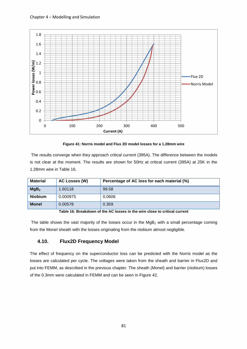
FIGURE 41: NORRIS MODEL AND FLUX 2D MODEL LOSSES FOR A 1.28MM WIRE .............................................................. 81
FIGURE 42: AC LOSSES OF THE BARRIER (NIOBIUM) AND SHEATH (MONEL) OF THE 1.28MM WIRE AT DIFFERENT FREQUENCIES
USING THE FEMM MODEL ................................................................................................................................ 82
FIGURE 43: AC LOSSES OF THE MGB2 1.28MM MONEL AND NIOBIUM WIRE AT DIFFERENT FREQUENCIES USING THE NORRIS
MODEL ........................................................................................................................................................... 82
FIGURE 44: AC LOSSES OF THE MONEL AND NIOBIUM IN THE 0.3MM WIRE AT DIFFERENT FREQUENCIES TAKEN FROM THE
FLUX2D MODEL .............................................................................................................................................. 83
FIGURE 45: AC LOSSES OF THE SUPERCONDUCTOR IN THE 0.3MM WIRE AT DIFFERENT FREQUENCIES USING THE NORRIS
MODEL ........................................................................................................................................................... 84
FIGURE 46: SUPERCONDUCTING CABLE MODEL ........................................................................................................... 95
FIGURE 47: INPUTS AND OUTPUTS OF THE SUPERCONDUCTING CABLE MODEL ................................................................. 96
FIGURE 48: SHOWS THE CONTOURS OF AN ELLIPTICAL WIRE ......................................................................................... 99
Chapter 1.3 – List of Abbreviations
7
1.3. List of Abbreviations
1-G First Generation Superconductor
2-G Second Generation Superconductor
AC losses Alternating Current losses
BCS Bardeen, Cooper and Schrieffer theory, explaining the process of a material
becoming a superconductor
BSCCO Bismuth Strontium Calcium Copper Oxide
EPRI Electric Power Research Institute
FEA Finite Element Analysis
FEM Finite Element Modelling
FEMM Finite Element Modelling Magnetics
HALE High Altitude Long Endurance
HTS High Temperature Superconductor
LIPA Long Island Power Authority
LTS Low Temperature Superconductor
MgB2 Magnesium Diboride
UAV Unmanned Aerial Vehicle
YBCO Yttrium Barium Copper Oxide
Chapter 1.4 – List of Symbols
8
1.4. List of Symbols
a Radius of core of model
A Vector potential
B Magnetic Flux Density
b Radius from centre of core to outer sheath in model
C Contour, concentric area of wire which is free of current
dr Infinitesimally small annular ring
E Electric field
Ec Electric field at critical current density
F Ratio of I/Ic
f Frequency
G Proximity effect loss factor
H Magnetic field strength
Hc Critical Magnetic field strength
I Current
I1 Current in core
I2 Current in sheath
Ic Critical current
J Current density
Jc Critical current density
k Boltzmann constant
L Inductance
L1 Total inductance in core
L12 Total mutual inductance between core and sheath
L2 Total inductance in sheath
Chapter 1.4 – List of Symbols
9
L0 External inductance to infinity
L∞ Inductance from sheath to infinity
Lc Energy lost per unit length
Lint Internal inductance of core
Lint2 Internal inductance of sheath
Lm Self-inductance of sheath
m The mth layer
M12 Mutual inductance between core and sheath
n The rate of transition for a current-voltage graph from zero to Jc
Qe AC loss caused by eddy currents
QH AC loss caused by hysteresis losses
Qmeas Total loss measured
QR AC loss caused by resistive losses
R Resistance
Rac,m AC resistance in the mth layer
Rdc,m DC resistance in the mth layer
R1 Resistance in core
R2 Resistance in sheath
T Temperature
Tc Critical temperature
V Voltage
Wm Magnetic field energy
ϕ Magnetic flux
μ0 Relative permeability
ρ Resistivity
σ Current density in Norris model, which is taken as a constant
Chapter 1.5 – Executive Summary
11
1.5. Executive Summary
This thesis represents the work undertaken by the author for an MPhil. The thesis is based on
investigating the feasibility of a superconducting cable in an aerospace electrical system. A
superconducting cable as well as a superconducting motor would increase efficiency and decrease
the weight of the electrical system.
The thesis begins with background information on superconductivity and then goes on to review
current literature. The literature review investigates current superconducting materials,
superconducting cables and superconducting AC losses. The review identifies MgB2 as a suitable
material for the application and goes on to identify AC losses as a major potential problem in making
superconducting cables in aerospace a viable option.
The main body of the report details the work undertaken on modelling and simulating the losses of
the sheath and barrier of a superconducting cable under different operating conditions. The model
was simulated at different currents and frequencies, as well as using different sheath and barrier
materials and configurations. The majority of the work was completed with the 2D finite-element
software, FEMM, but later modelling work was accomplished using Flux2D which includes a specific
superconducting module, allowing the superconducting material to be modelled more accurately.
By simulating the model in FEMM the influence of the proximity effect in the sheath/barrier of multi-
strand cables was investigated. It was found that although the proximity effect increased the losses; it
was negligible compared to the decrease in losses gained from using a multi-strand wire.
Using Flux2D enabled models of the superconducting core of the wire to be investigated as well as
the sheath/barrier. From the simulation it was found that at critical current and 50Hz the
superconductor was responsible for 99% of the AC losses. When the frequency was increased up to
800Hz for a 1.28mm Monel sheathed wire, however, the sheath/barrier losses were responsible for up
to 20% of the losses.
Chapter 1.6 – Declaration
12
1.6. Declaration
No portion of the work referred to in the thesis has been submitted in support of an application for
another degree or qualification of this or any other university or other institute of learning.
Chapter 1.7 – Copyright Statement
13
1.7. Copyright Statement
i. The author of this thesis (including any appendices and/or schedules to this thesis) owns certain
copyright or related rights in it (the “Copyright”) and s/he has given The University of Manchester
certain rights to use such Copyright, including for administrative purposes.
ii. Copies of this thesis, either in full or in extracts and whether in hard or electronic copy, may be
made only in accordance with the Copyright, Designs and Patents Act 1988 (as amended) and
regulations issued under it or, where appropriate, in accordance with licensing agreements which the
University has from time to time. This page must form part of any such copies made.
iii. The ownership of certain Copyright, patents, designs, trade marks and other intellectual property
(the “Intellectual Property”) and any reproductions of copyright works in the thesis, for example graphs
and tables (“Reproductions”), which may be described in this thesis, may not be owned by the author
and may be owned by third parties. Such Intellectual Property and Reproductions cannot and must
not be made available for use without the prior written permission of the owner(s) of the relevant
Intellectual Property and/or Reproductions.
iv. Further information on the conditions under which disclosure, publication and commercialisation of
this thesis, the Copyright and any Intellectual Property and/or Reproductions described in it may take
place is available in the University IP Policy (see
http://documents.manchester.ac.uk/DocuInfo.aspx?DocID=487), in any relevant Thesis restriction
declarations deposited in the University Library, The University Library’s regulations (see
http://www.manchester.ac.uk/library/aboutus/regulations) and in The University’s policy on
Presentation of Theses
Chapter 2 – Introduction
14
2. Introduction
The work is based around a High Altitude Long Endurance (HALE) aerospace vehicle. The HALE
Unmanned Aerial Vehicle (UAV) incorporated electrical propulsion using four 15kW wing mounted
electrical motors and a hydrogen fuel-cell as the electrical energy source. Hydrogen is more energy
dense than aviation fuel for the same weight, making it a good candidate for long endurance flights.
Hydrogen needs to be in gaseous form to act as a fuel and would, therefore, require a high volume.
This creates a problem for the UAV because it would need a large storage vessel to contain the
hydrogen. This storage vessel adds weight and volume, which impacts on the performance of the
UAV. If hydrogen is stored in liquid form, however, the volume can be significantly decreased and
hence the storage vessel can be significantly smaller and lighter.
Liquid hydrogen fuel would need to be converted back into gaseous form for the fuel cell, the liquid,
therefore, needs to be heated. The simplest method would be to use a heater to boil the liquid into
gas form. An alternative concept is to use the liquid hydrogen as a coolant for the propulsion motors.
This would perform the dual purpose of heating the hydrogen and allow the motors to be operated at
lower temperatures, increasing their efficiency. In this concept, the liquid hydrogen would need to be
distributed to the wing-mounted propulsion motors and it was proposed that the electrical cable could
be located inside the fuel pipe to reduce the losses in the cable. The need also for low cable losses
and the availability of liquid hydrogen on the UAV meant superconducting cables could be used,
cooled down using the liquid hydrogen.
In an ideal DC system there would be no losses in the superconductor. For AC electrical systems on
the other hand, superconductors exhibit small hysteresis losses in the superconducting materials and
eddy current losses appear in the surrounding materials if they possess any electrical conductivity.
This thesis examines AC electrical architectures and assesses the impact of AC losses on the
system.
Superconducting cables themselves could become an important part of aerospace electrical
systems, as the industry moves towards ‘more-electric’ aircraft .This work focusses on how the
superconductor and its sheath and barrier are affected by different currents and frequencies.
Chapter 3 –Literature Review
15
3. Literature Review
3.1. Introduction
The literature review is split into 4 parts: the history and theory of superconductivity; superconducting
materials; superconducting cables; and a review of AC losses in superconducting wires. It is useful to
understand the principles behind superconductivity and the history of superconductivity leading into
the theory of superconductivity, including the BCS theory and the debate surrounding the theory for
Type II superconductors. This thesis will concentrate on the superconducting materials which are
commercially available. The advantages of superconducting cables over conventional cables will be
examined. This chapter will also look at AC losses in superconductors and how these affect the
design of superconducting cables.
3.2. History and Theory of Superconductivity
A superconductor is a material that, when certain criteria are met, exhibits zero DC resistance and a
very small AC resistance. The state of superconductivity was discovered by Kamerleigh Onnes in
1911, when Onnes first liquefied helium down to temperatures of 1K and began to test the resistance
of different materials at that temperature [1]. At the time it was postulated that as the temperature
would drop, the resistance would also drop at the same rate. However, while testing the resistivity of
mercury at around 4K, Onnes found that the resistance suddenly dropped until it exhibited no
measurable resistance. It was quickly discovered that several other metals and alloys also displayed
this property.
When a material, which is superconducting, is cooled down to its Critical Temperature, Tc, the
resistance rapidly drops to zero, as seen in Figure 1.
Chapter 3 –Literature Review
16
Figure 1: Impedance of a superconductor (niobium) against a normal conductor (Monel) (Columbus
Superconductors)
Figure 1 shows that when niobium reaches about 9K, the resistance suddenly drops to zero, as
opposed to the Monel (which is composed of up to 67% nickel, the rest being copper and small traces
of other materials such as iron) where its resistance slowly decreases in a relatively linear fashion.
When a current flows through a conventional conductor such as Monel, the electrons collide with both
the lattice and each other and pass on energy in the form of heat; we term this the resistance of the
conductor. When the temperature of a conventional conductor is lowered, the energy of each electron
decreases meaning less is transferred in terms of heat and the resistance also decreases. When the
temperature is dropped down to around absolute zero the resistance reduces linearly as the
vibrations of the ions in the lattice decrease until the impurities and grain boundaries in the material
limit how low the resistance goes. A superconducting material on the other hand will suddenly reduce
its resistance to zero at its critical temperature.
When the niobium displays zero resistance it is in a superconducting state while at any temperature
above 9K it shows resistive qualities, which is known as its “normal” state. It was found that there are
three ways to “quench” a superconductor and return it to a normal state, from a superconducting
state. This occurs if any of the following parameters are exceeded:
Critical temperature, Tc
Critical magnetic field strength, Hc
Critical current density, Jc
If all three values are lower than the critical values the material will become superconducting as
illustrated in Figure 2.
0.00E+00
1.00E-07
2.00E-07
3.00E-07
4.00E-07
5.00E-07
6.00E-07
0 50 100 150 200 250 300 350
Imp
ed
ance
(o
hm
/m)
Temperature (K)
Monel
Niobium
Chapter 3 –Literature Review
17
Figure 2 : A figurative representation of the critical points for a superconductor [2]
3.2.1. Critical Temperature
There was no widely accepted theory to explain superconductivity up until 1957, when a group of
American scientists brought together their ideas and formed the BCS theory, so named after the
scientists, John Bardeen, Leon Neil Cooper and John Robert Schrieffer. The BCS theory explained
how a material was able to become a superconductor.
When an electron in a superconductor travels through the lattice of the material it attracts positively
charged ions in the lattice (phonons), which distort the lattice towards the electron. This distortion
attracts another electron of opposite spin. This attraction can overcome the Coulomb repulsion
between each electron. The two electrons become correlated and are known as cooper pairs. The
cooper pair electrons are the charge carriers and their charge q, is equal to twice that of a single
electron. The many cooper pairs tend to coalesce into a condensate where there are many pairs
together. This is known as a Bose-Einstein condensate. As the electrons travel around the lattice in
this condensate, the energy needed to break up these cooper pairs is greater than the individual
energy needed to break up the pairs if they were not in the condensate, this is known as the energy
gap. As the cooper pairs do not interact which the lattice they do not dissipate any energy as they
travel through the lattice. The electron condensate is classed as a “superfluid”. The cooper pairs are
only broken up when there is enough energy (whether thermal, magnetic or electrical) in the lattice to
break up all the pairs in the condensate (in the case of thermal energy this point being the critical
temperature). The energy gap needed to break up a pair is:
3.2 1
where k represents the Boltzmann constant and Tc is the critical temperature of the superconducting
material. The critical temperature is a key value for all superconductors, as one of the biggest
difficulties and costs comes from cooling the superconductor to below its critical temperature.
Chapter 3 –Literature Review
18
3.2.2. Critical Magnetic Field
A material in the superconducting state will return to a “normal” state when a “sufficiently strong
magnetic field is applied” [1]. This value is known as its Hc, as mentioned earlier. In 1933, Walther
Meissner and Robert Ochsenfeld discovered that a superconductor will repel all magnetic fields. This
effect is now known as the Meissner effect. When a material is superconducting it expels all magnetic
fields from its interior, displaying perfect diamagnetism. This effect is caused by circulating surface
currents which cancel all the flux density inside the superconductor by being the exact equal and
opposite flux density to the applied magnetic field [1]. For aerospace cables, large external fields are
not expected, so this critical value should only be influenced by the self-field of the cable current.
3.2.3. Critical Current Density
The critical current density is not an intrinsic property of a superconductor and is dependent on a
number of factors, which include the temperature of the superconductor and the size of the conductor.
The critical current density increases as the temperature reduces below the critical temperature. The
critical current density also reduces as the superconductor area increases. There would have to be a
compromise with regards to how far below the critical temperature the superconductor should
operate, as the temperature reduces the critical current density increases but the cooling costs also
increase. A quench due to excessive current occurs when the kinetic energy of the cooper pairs is
greater than the binding energy of the pairs. This is known as the de-pairing current density [1]. The
critical current is the current at which a certain superconducting wire will quench. This is
approximately the critical current density multiplied by the cross sectional area in which the current
flows through the wire. The critical current density is crucial for the development of superconducting
cables and as the critical current density increases the area of the superconducting wire needed
reduces which would save on costs.
For a superconductor to stay in the superconducting state, from the discussion on critical values
above, it is clear that the values are interdependent and each critical parameter has to be taken into
account.
3.2.4. Type II superconductors
Superconductors themselves can be broken up into two groups; Type I superconductors and Type II
superconductors. The superconductors that obey the BCS theory described earlier are called either
Low Temperature Superconductors (LTS) or Type I superconductors. Type I superconductors tend to
be pure elements or alloys and have low critical values.
Before 1986, 30K was theoretically believed to be the highest critical temperature a superconducting
material could achieve, until IBM researchers Karl Müller and Johannes Bednorz discovered the first
copper based High Temperature Superconductor (HTS) (also known as Type II superconductors)
earning them a Nobel Prize in 1987. This new group of superconductors could have a critical
temperature as high as 135K and could theoretically be as high as 165K [3]. This new group of
Chapter 3 –Literature Review
19
superconductors was found to have not only a higher critical temperature but also a higher critical
current density and critical magnetic field.
Another key difference between the two types is that HTS also have a so called vortex state. When a
Type I superconductor changes state from normal to superconducting or vice versa it is an instant
process, while a Type II superconductor goes through what is known as a transition phase. This
transition phase occurs when the superconductor is close to its critical magnetic field. Vortices of
normal material are created by lines of magnetic flux penetrating the material. These vortices are
surrounded by a circulating super-current. More of these vortices appear the closer a superconductor
gets to critical magnetic field and they begin to coalesce until the whole conductor is normal.
As no flux can penetrate a Type I superconductor it only has one Hc but Type II superconductors
have two values: Hc1 and Hc2. Hc1 occurs when a Type II superconductor enters the transitional, vortex
state. Whilst Hc2 is the limit before the superconductor quenches and becomes normal. Because flux
lines can penetrate a certain depth into a Type II superconductor (this depth is known as the London
penetration depth λ) structural anomalies, impurities and grain boundaries cause some of these flux
lines to become pinned in place and form vortices. Because of the Lorentz force, the vortices have a
force acting on it at right angles to both the current going through the superconductor and the flux.
This is known as “flux creep”. This flux creep decreases the critical temperature and critical current
density so many HTS materials have impurities added (known as doping) to increase flux pinning
(where the vortices are pinned in place) and this can increase all or one of the critical values. Type II
superconductors do not obey the BCS theory and there is not as yet a generally accepted theory
which explains how HTS materials work despite the fact they are widely used. It is these HTS
materials that this thesis will focus on: they are commercially viable and the higher critical values are
essential for a superconducting cable.
Chapter 3 – Superconducting Materials
20
3.3. Superconducting Materials
There are three main HTS materials that are currently used in most superconducting systems; these
are shown in Table 1.
Material BSCCO YBCO MgB2
Critical
Temperature
• 108K 93K 39K
Advantages • Liquid Nitrogen
cooled
High current
density
Liquid Nitrogen
cooled
Cheap
Easy to
manufacture
High current
density
Disadvantages Expensive
Hard to form
into wires
Lowest current
density
Expensive
The most
difficult to
manufacture
Difficult to form
into wires
Lower Critical
Temperature
Table 1: Advantages and disadvantages of the different superconductors on the market
Material Critical Temperature, Tc, (K) Critical Current Density, Jc, at 4.2K
(A/cm) and self-field in wires and
tapes
BSCCO
108 ~10E+06
YBCO
93 ~10E+07
MgB2
39 ~10E+07
Table 2: Critical values of the 3 most widely available superconductors ([4], [5], [6], [7], [8])
Table 2 compares the data for the three different materials. The table shows approximate values as
the samples tested sometimes were of different shapes and sizes and the measurement can differ.
3.3.1. BSCCO
Bismuth Strontium Calcium Copper Oxide (BSCCO) was the first HTS to be discovered that did not
contain a rare earth element and is the most studied superconductor. From Table 1 it can be seen
Chapter 3 – Superconducting Materials
21
that BSCCO has the highest critical temperature of the three HTS materials discovered. BSCCO was
the first HTS to be made into tapes and wires and these are called first generation (1-G) wires and
tapes.
The other HTS tend to be preferred as the elements that make up BSCCO are expensive and it is a
difficult and expensive process to make tapes and wires.
3.3.2. YBCO
Yttrium Barium Copper Oxide (YBCO) was the first material to achieve superconductivity above 77K
(the boiling point of liquid nitrogen.) Despite this it is known as a second generation (2-G) HTS. It has
a high critical current density and the fact its critical temperature is above the boiling point of liquid
nitrogen is a major advantage as with BSCCO. However it can only be produced in thin film form on a
coated conductor as it is extremely brittle and its critical current density reduces dramatically when
produced using the same method as BSCCO. Because of the difficulty in manufacturing YBCO into a
wire it is expensive even though its raw materials are relatively cheap. This is currently the most
widely used superconductor.
3.3.3. Magnesium Diboride
Superconductivity in Magnesium Diboride (MgB2) was only discovered in 2001. Its discovery was met
with some surprise not only for the fact that it had been sitting in chemistry labs for decades but also
because it was the first Type I superconductor with a critical temperature over 30K. This was thought
not to be possible according to the BCS theory. The reason for the unusual behaviour of MgB2 was it
possessed a double band gap. A superconductor band gap is seen as the energy needed to break up
the cooper pairs. One set of band gap electrons in MgB2 are much more superconducting than the
other and has a much higher critical temperature than the other, which means the critical temperature
of 39K is a compromise between the 2 different band gaps. However, because it obeys the BCS
theory but also has a vortex state it has been denoted a Type 1.5 superconductor [9].
MgB2 has a lower critical temperature than other HTS materials but the key advantage is that “MgB2
is a relatively simple compound of two abundant, inexpensive elements”[10]. It is also particularly
malleable so can be made into lengths of wires and tapes relatively easily when compared to YBCO
and BSCCO. The critical current density in wire form has very recently been increased as shown by
[8]. Wires are seen as advantageous as they are seen to be more adaptable, are easier to produce
and they tend to have lower transport AC losses. The transport AC losses are proportional to
width/radius which tends to be smaller in wires. For example, the width of a recent Columbus tape
tested was 2.84mm while the largest cylindrical wire tested was 1.28mm in diameter.
Although its constituents are cheap due to the fact that it does not contain rare earth elements like
YBCO and BSCCO, the fact that it has to be cooled to a lower temperature than the other HTS
materials means that it is a more expensive to keep MgB2 superconducting. The fact that a cryogen in
Chapter 3 – Superconducting Materials
22
the form of liquid hydrogen is available on the HALE UAV platform and is in liquid form below the
critical temperature for MgB2, means that MgB2 becomes a viable superconducting option.
Material Nominal operating
temperature (K)
Approximate material
cost
Through life cooling
(energy to remove 1W
of heat)
BSCCO 77K ~$200/kA.m 10W
YBCO 77K ~$250/kA.m 10W
MgB2 25K ~$5/kA.m 30-100W
LTS 4K ~$1/kA.m 1000W
Table 3: Comparison of costs for superconducting materials as of 2008 [4]
Table 3 shows the costs, as of 2008 but due to recent technological advances and greater demand
the cost of cooling has decreased for all of the materials listed. The prices of the superconducting
materials themselves have also decreased with Hyper Tech. Research Inc. expecting to be able to
sell MgB2 at below $1/kA.m in the near future [11]. One of the key considerations when it comes to
using superconductors is the cost of cooling the superconductors to below their critical temperature.
The lower the temperature, the higher the amount of energy needed to cool the material down to the
required temperature, which means an increase in cost. But as both BSCCO and YBCO use liquid
nitrogen, which freezes at 77K, the cost of cooling is reduced when compared to LTS materials which
require liquid helium (which freezes at 4.2K.) However the increasing costs are not linear with the
increase in cooling as can be seen in Figure 3.
Chapter 3 – Superconducting Materials
23
Figure 3: Costs of cooling against temperature (courtesy of American Superconductor Inc.)
As well as the cost of cooling another consideration is cost of the actual cryogen, which is down to
the cost to produce the cryogen and how common the cryogen is. Helium is difficult and expensive to
create artificially and because it is such a light element, the naturally created helium escapes our
atmosphere. This has led to an increase in rarity and has increased the costs leading many traditional
users of LTS looking at HTS, enabling them to use liquid hydrogen or nitrogen.
Despite being abundant, hydrogen on earth, only exists in compound form and has to be extracted.
To extract hydrogen a number of options exist but the vast majority (~90%) is produced by steam
reforming of methane. When compared to liquid helium a litre of liquid hydrogen is ~1/6 of the price
[12]. An advantage of using hydrogen over nitrogen is at ~20K an equivalent HTS can carry at least
several times the current of a HTS at 77K [13].
A key consideration in using MgB2 is the fact that as it is a relatively new superconducting material
and there is a lot of technological progress being made in improving its current density. The current
generation of wire has a current density of around ~ 1400 A/mm2 but the new 2
nd generation wire
being developed by Hyper Tech Inc. could have current densities of 10 times that as shown Figure 4.
Chapter 3 – Superconducting Materials
24
Figure 4: Improved characteristics of the 2nd
generation MgB2 wire (courtesy of Hyper Tech Research Inc.
[14])
Hyper Tech Research Inc. has only managed to produce small lengths of the 2nd
generation wire to
date, but is hoping to produce km lengths in the near future.
MgB2 reacts with oxygen, therefore, a protective sheath must stop any exposure to the atmosphere.
Monel, copper, titanium and stainless steel are commonly used as sheaths. The sheaths we are
focussing on are Monel and stainless steel, as these materials are relatively cheap and are relatively
easily moulded around the core MgB2. Monel is made up of approximately 67% nickel with the rest
being mostly copper. MgB2, however, also reacts with copper so a niobium barrier between the Monel
and the MgB2 is necessary. Niobium is also a superconductor but only below 9.2K and has high
conductivity in its normal state. Monel has a higher conductivity than stainless steel (3.3MS/m
compared to 1.84MS/m respectively) which means it would be more suitable for a monocore multi-
strand cable.
4.2K
Chapter 3 – Superconducting Materials
25
Figure 5: A mono-core MgB2 wire with a stainless steel sheath (Courtesy of HyperTech Inc.)
Figure 6: A multifilament tape with MgB2 filaments surrounded by a niobium barrier, in a Monel sheath
(Courtesy of Columbus)
Figures 5 and 6 show a mono-core stainless steel wire with MgB2 in the centre and also a
multifilament Monel tape showing the Monel sheath and MgB2 filaments each surrounded by a
niobium barrier. An 18 filament 0.8mm multifilament wire from Hyper Tech Research Inc. can be seen
in Figure 7. The picture is taken from [11] which goes on to talk about the advances in MgB2 and
gives an overview of its possible applications.
Monel
Niobium MgB2
Chapter 3 – Superconducting Materials
26
Figure 7: 0.8mm multifilament wire from Hyper Tech. Research Inc.
Chapter 3 – Superconducting Cables
27
3.4. Superconducting Cables
There has been little research undertaken on superconducting cables in aerospace systems.
However, there has been research undertaken on classical transmission superconducting cables. The
techniques, materials and technology documented for classical distribution systems can be assessed
for applicability to aerospace systems. Superconducting cables for transmission networks have only
recently been deemed to be financially beneficial and technically feasible. There is, however, no
single, tried and tested design for the cable. Multiple design concepts exist with various advantages
and disadvantages, however, all the designs are based on using BSCCO or YBCO and use liquid
nitrogen as a coolant [15]. However, recently CERN have built a 20m MgB2 transmission cable and
managed to obtain the highest current recorded in a superconductor (at the time of writing) of 20kA,
using liquid helium to cool the cable down to 24K [16].
The transmission cable itself has a number of design requirements it must satisfy:
The cable must be cooled below its critical temperature, Tc, and be at a stable temperature
along its length
It must have low AC losses
It must be protected from natural and man-made disturbances
It must not leak cryogen as this could be hazardous and it could cause damage to the
surrounding area.
Although AC systems are the focus of this investigation DC transmission is also a viable option but
this would require a different cable design.
There are two main types of superconducting AC cables; warm dielectric and cold dielectric. A warm
dielectric design is defined as a cable where the dielectric material is outside the liquid nitrogen.
Whilst a cold dielectric design means the dielectric material is placed in the liquid nitrogen where it
also acts as part of the dielectric insulation. Figure 8 shows a warm dielectric design and Figure 9 the
cold dielectric design.
Chapter 3 – Superconducting Cables
28
Figure 8: Warm dielectric cable design [17]
Figure 9: Cold dielectric cable design [17]
Chapter 3 – Superconducting Cables
29
The HTS shield layer seen in both Figures 8 and 9, supports the return current and shields the HTS
tape. The gap between the inner and outer insulators would be vacuum to limit heating of the
superconductor.
The warm dielectric cable is a standard AC cable re-designed to accommodate a superconducting
cable. The cold dielectric is a more recent design and was designed specifically for a superconducting
cable. The cold dielectric cable design had higher transport currents and more HTS tape/wire was
needed compared to the warm dielectric design. This was due to a screening layer which is formed
around the insulation using superconducting wires which ‘shields’ each phase and greatly reduces
stray electromagnetic fields emanating from each phase [17]. The warm dielectric design would be
easier to implement as it based on current designs and the cold dielectric design is dependent on
advancement in dielectric materials. However, the cold dielectric design tends to be preferred over the
warm dielectric design due to fact the ‘shielding’ means the external magnetic field is greatly reduced
which results in lower AC losses and lower inductance. The cold dielectric design also results in the
inductive impedance being six times lower than a conventional underground cable [15]. The other
advantage is the fact the cryostat is at ground potential, this means it can be maintained in the field
and there is easier access to the cable.
Some cable designs incorporate so called “quench conductors” [18] which is a layer of copper
surrounding the HTS which carries the current if the HTS quenches. Parts/all of the HTS become
resistive in the event of a quench and this would cause the current to transfer to the copper. This
temporary transfer of the current limits the temperature rise of the HTS material and allows it to return
to its superconducting state faster.
Conventional AC systems have 3 phases and the first cable designs had three separate single phase
cables. These single phase cables use the cold dielectric design and can carry a very high voltage.
Recently a different design has been developed called a “tri-axial” design (see Figure 10 and 11)
where “three phases are wound concentrically on a single core.” The advantage of this design is that
half as much superconducting material is needed [18] and as it is based on the cold dielectric design,
it has the same advantages over the warm dielectric design. This design tends to be preferred in
medium voltage applications.
Chapter 3 – Superconducting Cables
30
Figure 10: Showing the Triaxial design with “nitrogen impregnated, cold insulation between layers” [18]
Figure 11: Triaxial cable design [17]
The authors of [17] look at the problems and possible solutions for certain aspects of a HTS cable.
They point out that because warm dielectric cable designs have no electromagnetic screening, they
Chapter 3 – Superconducting Cables
31
generally have higher electrical losses and cable inductance compared to both the triaxial and cold
dielectric design. They also point out that the warm dielectric design is easier to realise as it is based
on current conventional cable design. The cold dielectric design is more ambitious and would need
further developments in terms of dielectric materials, terminations and joints. They continue to point
out that as the dielectric material is impregnated with liquid nitrogen it must not boil in order to
maintain its dielectric strength. The authors identify another major obstacle of using long lengths of
superconducting cable, which is the cooling system has to evacuate the heat of the losses over what
could be a very long length of cable. The paper concludes that the volume of the HTS tape required is
small compared to the rest of the components in the cable. Most of the cable volume is taken up by
the vacuum space, copper stabilisation layers, dielectric and liquid nitrogen.
Maguire and Schmidt et al [19] describe the installation and test results of the Long Island
transmission level HTS cable. The cable is made up of three single-phase cold dielectric cables,
600m long. The cable system was designed to carry 574MVA at a voltage of 138kV. It was also
designed to self-limit a 51,000 Arms fault for 200 milliseconds. It was successfully connected to the
Long Island Power Authority (LIPA) grid in 2009. The cable uses a 1-G BSCCO wire cooled in liquid
nitrogen. The BSCCO wire had a critical current of 135 A per wire for a 4.3mm wide conducting layer,
the shield layer present had a critical current of 105 A. There was approximately 155km of
superconducting wire in the cable system. The LIPA cable is currently the longest superconducting
cable, with the highest voltage rating under test. The paper demonstrates the feasibility of
superconducting cables in transmission systems
Maguire and Yuan et al [20] continue the work on the LIPA project. This paper describes the
progress and status of the installation of a 2-G HTS power cable in the LIPA grid. The project named
LIPA II was developed to replace one of the phases with a 2-G YBCO conductor and to demonstrate
a commercial cable system is viable. The paper details another reason for replacing the BSCCO wire
with the YBCO coated conductor is the fact they want to be able to demonstrate a fault limiting design
as well as a fault tolerant design. The fault tolerant design has already been demonstrated with the 1-
G BSCCO cable but due to its low resistivity when non-superconducting (normal) it cannot limit a fault
while the YBCO conductor can limit the fault current. The authors also looked at various aspects of
the cable system that they thought might prove problematic. The paper successfully tested the idea of
a field cryostat that could be repaired even in very severe cases of damage and contamination. They
went on to successfully test a cable joint and a modular high efficient refrigeration system. The paper
again proved the validity of various aspects of the superconducting cable design, including fault
limiting design and a cryostat that could be repaired without being taken out of the network.
Eckroad et al [18] looked at the design of an interregional, superconducting DC cable system in the
US that is intended to deliver 10GW power capacity and nominal current and voltage of 100kA and
100kV respectively. They highlight the advantages of using DC superconducting cables over long
distances. Overhead AC long distance transmission cables are unsuitable because of the losses from
requiring increased voltage levels. They proposed using an underground DC superconducting cable
which would ideally be completely lossless and they claim it would be available at lower cost as they
Chapter 3 – Superconducting Cables
32
require only two cables lines instead of three. It would also be more reliable and space effective being
underground. However, the cables would need to be larger and any change in current would result in
the cable no longer being DC meaning there would be some AC losses. The paper points out that the
cost effectiveness of using DC increases as the distances increase, even with the added cost of the
requires AC-DC converters. Due to the fact that losses in all forms of AC transmission increase with
the power transmitted compared to superconducting DC cables, the authors point out that it is most
suitable to use the DC superconducting cable at higher power levels where the percentage of losses
would be substantially less. This is where superconducting cables would be most advantageous; long
distance and high power. The difficulties however in maintaining the temperature and vacuum over
long distances would need to be overcome.
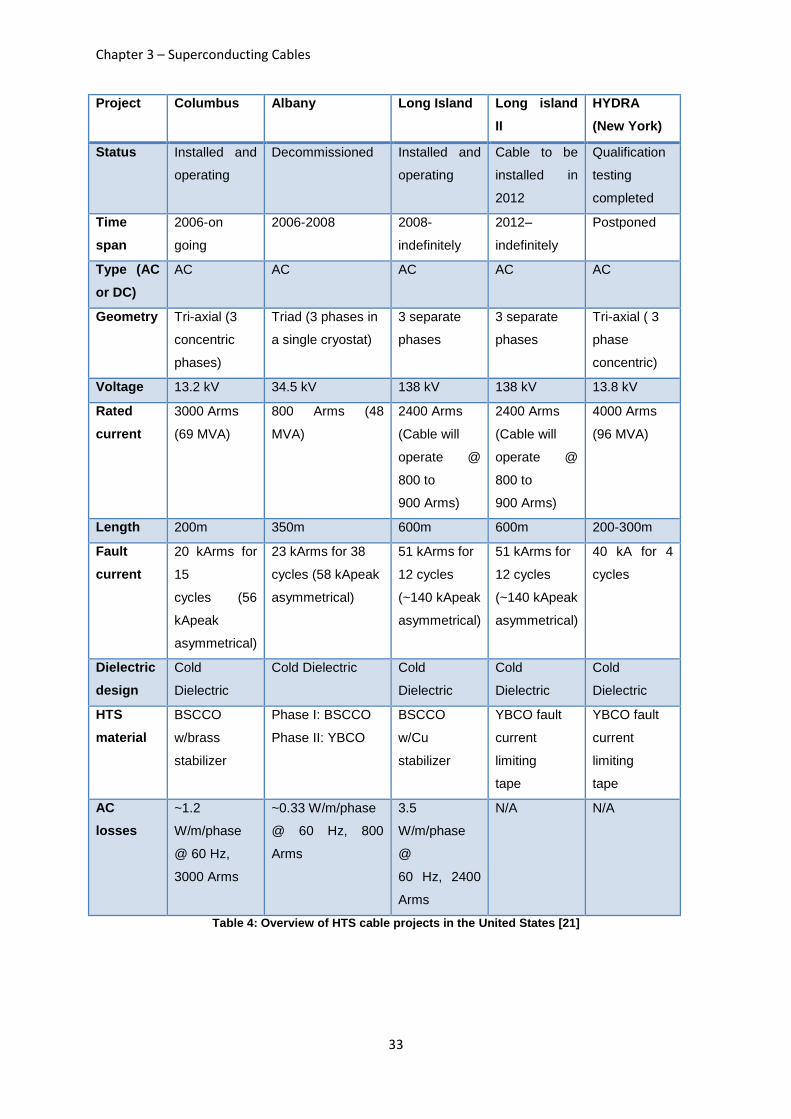
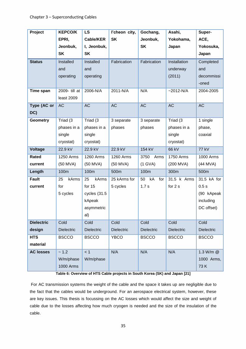
Young et al [21] have published an EPRI report comparing the progress and development of current
superconducting power cable programs around the world. Tables 4, 5 and 6 are taken from this report
and are shown below.
Chapter 3 – Superconducting Cables
33
Project Columbus Albany Long Island Long island
II
HYDRA
(New York)
Status Installed and
operating
Decommissioned Installed and
operating
Cable to be
installed in
2012
Qualification
testing
completed
Time
span
2006-on
going
2006-2008 2008-
indefinitely
2012–
indefinitely
Postponed
Type (AC
or DC)
AC AC AC AC AC
Geometry Tri-axial (3
concentric
phases)
Triad (3 phases in
a single cryostat)
3 separate
phases
3 separate
phases
Tri-axial ( 3
phase
concentric)
Voltage 13.2 kV 34.5 kV 138 kV 138 kV 13.8 kV
Rated
current
3000 Arms
(69 MVA)
800 Arms (48
MVA)
2400 Arms
(Cable will
operate @
800 to
900 Arms)
2400 Arms
(Cable will
operate @
800 to
900 Arms)
4000 Arms
(96 MVA)
Length 200m 350m 600m 600m 200-300m
Fault
current
20 kArms for
15
cycles (56
kApeak
asymmetrical)
23 kArms for 38
cycles (58 kApeak
asymmetrical)
51 kArms for
12 cycles
(~140 kApeak
asymmetrical)
51 kArms for
12 cycles
(~140 kApeak
asymmetrical)
40 kA for 4
cycles
Dielectric
design
Cold
Dielectric
Cold Dielectric Cold
Dielectric
Cold
Dielectric
Cold
Dielectric
HTS
material
BSCCO
w/brass
stabilizer
Phase I: BSCCO
Phase II: YBCO
BSCCO
w/Cu
stabilizer
YBCO fault
current
limiting
tape
YBCO fault
current
limiting
tape
AC
losses
~1.2
W/m/phase
@ 60 Hz,
3000 Arms
~0.33 W/m/phase
@ 60 Hz, 800
Arms
3.5
W/m/phase
@
60 Hz, 2400
Arms
N/A N/A
Table 4: Overview of HTS cable projects in the United States [21]
Chapter 3 – Superconducting Cables
34
Project Amsterdam,
Holland
InnoPower,
Kumning, China
Changong,
Lanzou, China
Moscow, Russia
Status Development Installed and
Operating
Operating Development
Time
span
TBD 2004- N/A 2004-N/A Installation in 2012
Type (AC
or DC)
AC AC AC AC
Geometry Tri-axial (3
concentric
phases)
3 separate phases 3 separate
phases
3 separate phases
Voltage 50 kV 35 kV 6.6 kV 20kV
Rated
current
2900 Arms
(250 MVA)
2000 Arms
(120 MVA)
1500 Arms
(17 MVA)4
2000 Arms
(70 MVA)
Length 6km 33.5m 75m 200m
Fault
current
20 kA
20 kArms for 2 s
(27 kApeak
asymmetrical)
N/A N/A
Dielectric
design
Cold Dielectric Warm Dielectric Warm Dielectric Cold Dielectric
HTS
material
TBD BSCCO
BSCCO
BSCCO
AC
losses
TBD ~1 W/m/phase
@ 50 Hz, 74K,
1500 Arms
> 0.42–0.85 W/m/
phase @ 50 Hz,
1500 Arms
N/A
Table 5: Overview of HTS cable projects in Europe, China and Russia [21]
Chapter 3 – Superconducting Cables
35
Project KEPCO/K
EPRI,
Jeonbuk,
SK
LS
Cable/KER
I, Jeonbuk,
SK
I’cheon city,
SK
Gochang,
Jeonbuk,
SK
Asahi,
Yokohama,
Japan
Super-
ACE,
Yokosuka,
Japan
Status Installed
and
operating
Installed
and
operating
Fabrication Fabrication Installation
underway
(2011)
Completed
and
decommissi
-oned
Time span 2009- till at
least 2009
2006-N/A 2011-N/A N/A ~2012-N/A 2004-2005
Type (AC or
DC)
AC AC AC AC AC AC
Geometry Triad (3
phases in a
single
cryostat)
Triad (3
phases in a
single
cryostat)
3 separate
phases
3 separate
phases
Triad (3
phases in a
single
cryostat)
1 single
phase,
coaxial
Voltage 22.9 kV 22.9 kV 22.9 kV 154 kV 66 kV 77 kV
Rated
current
1250 Arms
(50 MVA)
1260 Arms
(50 MVA)
1260 Arms
(50 MVA)
3750 Arms
(1 GVA)
1750 Arms
(200 MVA)
1000 Arms
(44 MVA)
Length 100m 100m 500m 100m 300m 500m
Fault
current
25 kArms
for
5 cycles
25 kArms
for 15
cycles (31.5
kApeak
asymmetric
al)
25 kArms for
5 cycles
50 kA for
1.7 s
31.5 k Arms
for 2 s
31.5 kA for
0.5 s
(90 kApeak
including
DC offset)
Dielectric
design
Cold
Dielectric
Cold
Dielectric
Cold
Dielectric
Cold
Dielectric
Cold
Dielectric
Cold
Dielectric
HTS
material
BSCCO
BSCCO
YBCO BSCCO
BSCCO
BSCCO
AC losses ~ 1.2
W/m/phase
1000 Arms
< 1
W/m/phase
N/A N/A N/A 1.3 W/m @
1000 Arms,
73 K
Table 6: Overview of HTS Cable projects in South Korea (SK) and Japan [21]
For AC transmission systems the weight of the cable and the space it takes up are negligible due to
the fact that the cables would be underground. For an aerospace electrical system, however, these
are key issues. This thesis is focussing on the AC losses which would affect the size and weight of
cable due to the losses affecting how much cryogen is needed and the size of the insulation of the
cable.
Chapter 3 – AC losses in Superconductors
37
3.5. AC Losses in Superconductors
AC losses are a significant factor in the design of superconducting cables; the losses directly affect
the cryogenic system which is a major factor in relation to cost and weight as well as difficulties in
maintaining a suitable temperature. AC losses along the cable effects the volume of insulation
required and also cryogen needed.
In this application the amount of cryogen needed (liquid hydrogen) on the aircraft is related to the
electrical energy required from the fuel cells and this is related to the losses in the cables and
propulsion motors. Although some AC losses would be useful to heat up the hydrogen, excessively
high AC losses would reduce the effectiveness of the hydrogen in cooling the superconducting
propulsion motors.
AC losses in a superconducting cable have a number of contributing factors: and the key loss
mechanisms are;
Hysteresis losses
Coupling losses
Eddy current losses
Proximity effect
Hysteresis losses are the largest contributors towards the AC losses and occur when a Type II
superconductor is in a mixed state. Energy is used in de-pinning and moving vortices when a
magnetic field is applied. Each AC cycle uses a certain amount of energy in moving the flux in and out
of the superconductor. This means that the hysteresis losses are proportional to frequency. “Flux
creep,” as described earlier, requires energy to keep the vortices moving through the material [1]. A
material can, therefore, be doped to increase flux pinning to decrease the hysteresis losses. The
hysteresis losses are influenced by the magnitude and direction of the external magnetic field and
also the penetration depth (London depth) of the superconductor and the geometry of the
superconductor.
Norris [22] describes two methods for calculating hysteresis losses in Type II superconductors. This
paper follows the assumption that the critical current density is independent of the magnetic field, this
is known as the London model. The model assumes that as the current increases above Tc, the
resistance of the superconductor rises sharply as the maximum critical current density is exceeded
and the “resistance is such that the ohmic voltage drop exactly balances the driving emf with the
current density remaining constant.” The author looked at the losses in different shaped wires and
different cross sectional areas and to see if the different shapes and cross sectional areas had any
effect on the AC losses. It was found that for solid wires with the same current carrying capacity, the
size or shape of the wire can only vary the losses by, at most, a factor of three. Losses at the edges
of thin sheets were also analysed and a fourth-power dependence on the current was found. The
Chapter 3 – AC losses in Superconductors
38
edges of the thin sheets were placed at different angles to the current and the losses were analysed.
The paper gave us a method of calculating the hysteresis loss in different shaped wires and tapes
through a model which is herein referred to as the Norris model. For the AC loss in a round or
elliptical wire we can use the equation:
3.5
Where Ic is the critical current, μ0 is the relative permeability and LN is a function of F which is given
by F= I/Ic and is shown in Table 7.
F, ratio given by I/Ic LN
0.1 5.6E-05
0.2 4.7E-04
0.3 1.7E-03
0.4 4.3E-03
0.5 9.1E-03
0.6 1.7E-02
0.7 3.0E-02
0.8 5.0E-02
0.9 8.4E-02
0.95 1.11E-01
0.98 1.34E-01
1 1.6E-01
Table 7: The LN value for different peak current values with respect to the critical current
The Norris model itself is based on the Bean critical state model. This paper is seen as an important
paper in calculating the AC losses in superconductors.
Bean [23] described a critical state model which is still widely used today and it is from this model
that the Norris Model is based. In the critical state model, Bean makes some key assumptions:
Up to the critical current density, Jc, it is assumed that the superconductor can carry current
without loss.
The critical current density, Jc, is independent of the magnetic field.
The lower magnetic critical field, Hc1, is zero.
All the flux vortices have the same Lorentz force applied.
When a current flows through the superconductor it flows at critical current in a small area
around the outer edge of the material. Increasing the current, simply increases the area
carrying critical current until the whole superconductor is carrying critical current. This current
is referred to as a supercurrent.
Chapter 3 – AC losses in Superconductors
39
The model only allows the material to be in two states: superconducting or a mixed state where some
parts of the material are superconducting and some are normal. Using these assumptions Bean was
able to derive the full hysteresis loop of a superconductor:
{
, 3.5 1
where J, is the current density, Jc is the critical current density, E is the electrical field and Ec is the
electrical field at critical current density. The equation shows that if a superconductor or part of a
superconductor has never been exposed to an electric field, then the current density is zero. If a
superconductor on the other hand has been exposed to an electric field the current density is equal to
the critical current density.
The Bean model assumes that the critical current is not linked to magnetic field. This was rectified
when [24, 25] together created the Kim-Anderson model. This model allows for the fact that the
magnetic field is linked to the critical current. Both the Bean model and later the Kim-Anderson model
are heavily used in numerical simulations and are used to simulate superconductivity in commercial
software (such as Flux 2D.) [26] States that the equation 3.5 1 can be used in numerical simulations
if it is re-formulated as:
⁄ If E ≠ 0 3.5 2
and
⁄ If E = 0 3.5 3
where T is the temperature dependence of the superconductor. The assumption made by Bean that
the flux exists in vortices is key to AC losses as these flux vortices cause the hysteresis losses which
are a large component of the total AC losses. The assumption means that the transition between zero
current and Jc is very fast which disagrees with experimental results on some superconductors.
Through a phenomenological approach and by experiments, the power-law relationship was found to
be consistent with the voltage-current characteristics of some Type II superconductors. In this model
the transition between zero and critical current density can be stated as:
(
)
3.5 4
where n represents the rate of transition for a current-voltage graph from zero to Jc. If n = 1 then the
material would be completely resistive and follow the normal conductor relationship ρ = E0/J0 where ρ
is the resistivity. If n = ∞, this would represent a perfect superconductor with zero resistance, where Jc
= J0 with a near “step change” transition to Jc. Changing the n value allows one to represent the whole
spectrum of superconductors. [27] The power-law is regarded as the most accurate way to model the
superconductors non-linear resistivity and is commonly used in software to model AC losses (e.g.
Flux 2D).
Chapter 3 – AC losses in Superconductors
40
The Finite Element method (FEM) is commonly used to calculate the AC losses in superconductors.
There are a variety of numerical and analytical methods for calculating the AC losses, however, this
thesis focusses on FEM. Today 2D FEM calculations are generally accepted as fully developed as
they are both accurate and quick [28].
FEM simulations are described by [29] as “minimising a ‘functional’, integrated over all space, which
for electromagnetism has the dimensions of energy and in some cases can be interpreted as the free
energy of the system”. The governing differential equations are used to derive the ‘energy-related
functional’ which is then minimised to obtain the solution. The advantage of this method is that it can
use a wide range of minimisation techniques which can then be used in many different situations.
Both [28] and [29] agree that formulating a superconductor as an eddy current problem is a reliable
method and that A-V, T-Ω and H formulations are the most common methods.
The A-V formulation, which is described well by [29], is based on the vector potential A, which has
three spatial components related to the current density vector and is the most common approach
used in magnetic problems. In 2D FEM solutions, A is reduced to a scalar with a single variable at
each node in the mesh. For 3D FEM solutions, A is a vector quantity so requires 3 variables at each
node. The magnetic vector potential, A, is defined if its curl and divergence are defined. The curl of A
is directly related to flux density defined by and . However we can use the
definition of the divergence of A to introduce a scalar potential term: , we can put
where V is the arbitrary scalar. The introduction of the scalar term V allows materials in
the problem with no currents flowing in them to be modelled using the single variable, V, at each node
and this significantly reduces the computational resources required. The equations use Maxwell’s
equation and from this we get ( ) and these equations are solved using most
commercial software. V is not needed in all situations, if the boundary is encountered by the currents
flowing along the applied E lines then both V and ( ) can be ignored. However, this is not
the case if the current circulates around a boundary [29].
The T-Ω formulation is similar but uses different electromagnetic variables. As then we can
define a vector potential by and also where Ω is the scalar
potential. Ω can be linked with magnetic surface poles in the same way that V is determined by
surface charges in the A-V formulation [29]. Both formulations are closely related but if there is no
ferromagnetic material present then Ω is zero, meaning this can no longer be used as a variable. As
each variable can increase computing requirements by a factor of 10, it means the T-Ω can be much
quicker in certain circumstances [29].
The H formulation is an eddy current problem similar to the other methods but has the advantage in
the fact that it is formulated directly using the magnetic field intensity, H, without any additional
potential functions which the other formulations use [30].
In [30] they find that while the A-V formulation is fast when the same mesh is used it needs a denser
mesh to get reliable results and that the H formulation is considered more intuitive. While [29] finds
Chapter 3 – AC losses in Superconductors
41
that the different methods have different advantages when used in different 2D Cartesian geometries
and how they are modelled with respect to J,A and B. The author also finds that the A-V formulation
has convergence problems and recommends using the T-Ω formulation.
Previous research has been done on AC losses in superconducting cables, however, most of this
has been focussed on AC losses in winding cables for magnets and is assessed mainly in regards to
the effect of large external fields. The superconducting cables in this application are not expected to
be exposed to any significant external fields. The literature review, therefore, will concentrate on
papers investigating superconducting AC losses in the presence of self-field.
Douine et al [31] compare analytical models with measured data on AC losses using BSCCO 2223.
The models used were the Bean critical state model and a numerical calculation in which the losses
were calculated using the distributions of the electric field (E) and the current (J). Both the models and
the measured losses were taken at 50Hz and between 60 and 100 Amps, with 100 Amps being the
superconductors critical current Ic. The data was taken at 77K and in self-field only. It was found that
the models and the data agree strongly as long as the current is below Ic. The authors conclude that
although the two models produce different distributions of E and J the AC loss values are very similar.
Young et al [32] found that a magnetic sheath increases the AC losses. They looked at how a nickel
sheath responded to self and applied magnetic fields at different frequencies (from 3-2000Hz.) They
tested two multifilament wires to look at the differences in AC losses; a nickel only sheath which is
magnetic; and a nickel and chromium sheath which was weakly magnetic. For the nickel sheathed
wire they found the AC losses in MgB2 to be independent of temperature. They also found the losses
were more than three orders of magnitude higher than the superconductor loss up to 10A but
increased almost linearly over 10A. The authors stated that his was representative of a ferromagnetic
hysteretic loss originating in the sheath.
Murase et al [20] measured the self-field loss in AC transport current of nickel-sheathed MgB2
superconducting tapes. The paper studied the transport loss against temperature, frequency and the
AC transport current for the nickel-sheathed superconductor. The effects of the ferromagnetic nickel-
sheath losses were also discussed. The experimental test used a lock-in amplifier which measured
the resistive voltage with an additional coil to eliminate the inductive voltages with a shunt resistor to
measure the current. The sample was tested at frequencies from 100Hz up to 2000Hz. The results
showed that compared to MgB2 non-ferromagnetic sheaths (such as stainless steel), the losses are
higher using the nickel sheath and they disagree further with the Norris model losses. The cause of
this extra loss is put down to the hysteresis loss of the ferromagnetic sheath which was examined
using FEM. The hysteresis loss of the nickel sheath was measured and found it made up a “few
percent of the total loss.” The paper also demonstrated that the MgB2 had essentially the same
superconducting properties regardless of the sheath materials. The paper claimed that the transport
losses were due to the inhomogeneity of the critical current density in the MgB2 core and the Norris
model would under-predict the losses as a result.
Chapter 3 – AC losses in Superconductors
42
Rostila et al [33] looked at reducing the AC losses in MgB2. They cite other papers stating high AC
losses can be attributed to ferromagnetic sheaths, such as; iron, nickel and Monel (which contains up
to 30% nickel.) To test a wire without magnetic properties they tested titanium sheathed multifilament
wire and compared it against it FEM software using vector potential formulation. The work focussed
on how a transverse magnetic field affects the AC losses with a non-magnetic sheath. They found
that the losses are dominated by the superconductor and that the filaments could be modelled
uncoupled unless they were densely packed.
Tanaka et al [34] looked into the AC loss properties of MgB2 multifilament wires. The authors
designed and manufactured a low AC loss multifilament wire and compared it to a standard
multifilament wire at different frequencies and magnetic fields. The standard wire had a copper sheath
and a niobium barrier. Copper was used because it is a good stabilizing material, highly conductive
and has low para-magnetism. The low AC loss multifilament wire had a copper-nickel sheath and a
tantalum barrier. They found that the AC loss was made up of a hysteresis loss from the
superconducting filament, a coupling loss between the filaments and an eddy current loss in the
sheath. The wire design was found to have lower AC losses at higher magnetic fields but it was only
tested at frequencies up to 5Hz.
Ainslie et al [35] compared the electrical measurements of transport AC losses in YBCO conductors
against 2D Finite Element Method (FEM) models. The experimental results were based on the
superconducting stator coils used in a superconducting permanent magnet synchronous motor
design. An electrical method was used as opposed to a calorimetric method which required extensive
calibration to isolate the AC superconductor loss from other losses. The experimental setup was
based on a lock-in amplifier. The YBCO conductor had a critical current of 100A and was tested at
50Hz immersed in liquid nitrogen. The experimental results were shown to correlate well with the 2D
FEM models.
Yang et al [21] (2005) carried out experimental tests to determine the effects of different shaped
wires and tapes on AC losses. The authors looked at bulk MgB2 (3mm x 0.5mm and 50mm long) and
a nickel sheathed MgB2 wire at temperatures between 25K and 40K in an applied field up to 0.2T at
59 Hz. The AC losses in the bulk conductor were found to increase with H4 until the MgB2 is
magnetically saturated when the increasing losses reduced considerably. When the width was
decreased to 1mm, its characteristics were more similar to that for a round wire varying as H3. The
authors claimed that below 35K the losses were unchanged so the losses were temperature
independent below the transition temperature. Testing a BSCCO wire inside a cavity of an iron
‘shielding block’ it was found to have very similar results to the nickel sheathed MgB2. The
researchers concluded that as the AC losses in a HTS were significantly reduced when in a magnetic
sheath because of the shielding effect of the iron block; the self-field loss becomes more important in
regard to the losses.
Coupling losses are another loss mechanism in superconductors. Coupling losses tend to occur in
multifilament tapes where the filaments are in close proximity to each other. When superconducting
Chapter 3 – AC losses in Superconductors
43
filaments or strands are parallel to each other and a perpendicular magnetic field is applied, the
filaments become magnetically coupled through mutual inductance. This induces eddy currents in the
resistive matrix around the superconductors and the fact that these currents have to travel through a
resistive matrix means there are also ohmic losses. The losses are proportional to frequency squared
and to the ‘looped area’ which means using smaller diameter superconductors reduces the losses
[36]. The closer in proximity the strands are, the higher the losses, therefore to reduce the coupling
losses by increasing the amount of smaller diameter strands used, the overall area of the tape would
have to increase to keep a sufficient distance between the strands. Coupling losses are also related
to the length of the cable as the longer the cable, the larger the ‘looped area’.
The coupling losses were found to be lower when the sheaths and barrier are relatively resistive
(such as stainless steel [37]) and the losses become independent of the length of the cable when in
parallel [38]. Experimental tests were undertaken in [39] on the effect of twisting multiple strands of
composite superconducting conductors and they found that twisted Nb-Ti-Zr filaments with a 2mm
pitch had zero magnetic coupling and the losses are equal to the hysteresis losses of filaments. The
advantage of using mono-core superconducting wire is the fact the superconducting cores are
physically much further apart compared to a multifilament wire or tape, thereby reducing the coupling
losses.
It is worth noting that the proximity effect in normal conductors should not to be confused with the
proximity effect in superconductors which occurs when the superconducting material is placed in
contact with a non-superconducting material. Where the two materials are in contact, the electrons
from the superconductor and the normal material cannot instantly interchange. Over very small
distances (in the orders of micrometres) the effect results in the normal material exhibiting some weak
superconducting properties while the superconductor displays some resistive properties. This small
reverse of properties results in a small loss in the superconductor and a small lowering in its Tc. This
is lowered further when the material that is in contact with the superconductor is ferromagnetic [40].
The proximity effect in normal conductors effects the sheath and barrier of the MgB2 wire. When an
isolated conducting wire carries an AC current it produces an alternating magnetic field, which will
create eddy currents in other conductors nearby. The eddy currents cause a re-distribution of the
conductor current. This increases the resistance of the conductor as a function of the frequency. The
losses are proportional to frequency squared.
To calculate the proximity in cables a number of methods are used. A review is completed in [41] of
all the articles at the time in which they compare the different methods available. All the methods are
related to transformer windings but are still useful for calculating the proximity losses in straight
cables. The papers also take into account the skin effect of the conductor and add this together with
the proximity effect to get the total eddy current losses in the windings. The paper states that the
methods devised in the Dowell[42] and Perry[43] articles form the basis of all the other papers in the
review. Both Dowell and Perry combine electromagnetic theory and MMF (MagnetoMotive Force)
diagrams to develop their method and make the same assumptions;
Chapter 3 – AC losses in Superconductors
44
The flux lines are parallel to the core of the transformer.
The layers of the conductor windings can be modelled as a single square conductor of the
same cross-sectional area for analysis.
The curvature of the transformer windings can be ignored when calculating the radial field
distribution across the winding layer. This means the single rectangular block of conductor
can be modelled as pieces of infinite current sheets.
The capacitive effects in the windings can be neglected.
The magnetic field outside each layer is negligible.
Dowell’s method only applies to winding portions which are defined “as a portion of the winding
where the magnetic field intensity is zero and extends in either direction until the magnetic field
reaches a positive or negative peak”. Dowell and subsequent authors went on to develop the method
where they calculate the proximity effect factor (G) [44]. The round conductor with a diameter of d is
replaced with by a square conductor with the same cross-sectional area, with its width being equal
to√ . G can be gained from:
3.5 5
where ξ is defined as:
√
3.5 6
where δ is the skin depth which can be defined as
√
3.5 7
where μ is the relative permeability, ω is the angular frequency and σ is the conductivity of the
material. When Dowells method is combined with findings from [45] the proximity effect losses in a
single winding layer at one frequency can be seen as:
[( ) ] 3.5 8
where A is the surface area of the conductor, H is the highest magnetic field intensity applied to the
either side of the winding. Hr is the magnetic field ratio from the highest side of the conductor to the
lowest. Mn and Dn are defined as:
( ) ( )
( ) ( ) 3.5 9
( ) ( ) ( ) ( )
( ) ( ) 3.5 10
Chapter 3 – AC losses in Superconductors
45
where Φ can be described by
3.5 11
For a non-sinusoidal waveform equation 3.5 9 must be applied to each significant harmonic. When
the Dowell method is combined with the skin effect expression and the current density distribution in a
single winding of an infinitely long current sheet the AC resistance in the mth layer can be expressed
as:
[
( )
] 3.5 12
where Rdc,m is the DC resistance of the winding, while Rac,m is the AC resistance of the winding and m
is the number of the winding being considered. However this method is said to be inaccurate at high
frequency by [44] as when replacing the round conductor with the square conductor the AC resistance
of the square conductor is underestimated at high frequency. The authors further try to fit their results
with Finite-Element Analysis (FEA) simulations by introducing two coefficients; k1 and k2 into the
Dowell function:
√ (√ ) (√ )
(√ ) (√ ) 3.5 13
where X is defined as
3.5 14
The authors normalize G against applied field and material conductivity making it unit-less. FEA
simulations can predict the proximity effect losses to as a high as accuracy as needed although the
simulation can be time consuming and will only be correct for the specific parameters set. Both FEA
and the modified Dowell method can be time consuming and complicated. In this thesis predicting the
proximity effect loss factor in less accurate but simpler and quicker way will be investigated.
It is possible to break down the different kinds of losses to see how they are affected by frequency.
Stavrev et al [46] looked at the losses in BSSCO 2223, breaking the losses down into three parts:
Hysteresis (QH), eddy current (Qe) and resistive losses (QR) as follows:
3.5 15
where Qmeas is the total loss measured. The equation shows, as expected, the eddy current loss has
a quadratic dependence on frequency while the hysteresis losses are linear and the resistive losses
are constant. The testing was done at relatively low currents. The results show good agreement with
measured results. They also found that the fill factor of the superconductor and changing the
geometries of different wires were the biggest factor in relation to the loss, while the sheath thickness
had little impact on the losses. The paper concluded that at high applied currents of (> 80% of critical
Chapter 3 – AC losses in Superconductors
46
current ratio) a resistive loss results from the flux creep in the superconductor. For lower frequencies
(<100Hz) the resistive losses make up a large part of the losses (30-40%) whilst above it the resistive
losses are negligible. The paper concluded that the hysteresis losses up to 1 kHz make up the
majority of the losses. Although the eddy current losses depend on the square of the transport
current, the proportion of loss gets smaller as the current ratio (applied current to critical current)
increases.
Two options were available when it came to deciding which wire to model, these being a
multifilament wire or a mono-core wire. Multifilament wires have multiple filaments of MgB2 running
through the wire and tend to be in tape form. The filaments are twisted inside the tape as this reduces
the AC losses when a magnetic field is applied. While mono-core wires tend to be cylindrical and
have a single filament of MgB2 running throughout the wire. Multifilament tapes were originally
designed to reduce ‘flux jumping’ in MRI magnets in Nb3Sn and NbTi. Flux jumping occurs when a
superconductor is fully magnetised but part of the superconducting wire is thermally disturbed by
motion or AC loss or a hotspot where there is a defect. This hotspot has a lower critical current
density than the other wires therefore it will heat up and eventually turn normal, if there are multiple
wires the higher current will flow into the other wires. This causes a change in the screening current
and increases the Jc which allows flux penetration which again increases the Jc and thus increases
heating until all the wires are normal. However, this is shown not to occur in MgB2 [47] as flux jumping
is shown to be dependent on temperature and MgB2 has a higher Tc than LTS.
The multifilament tape design reduces losses from large applied parallel fields, however as
aerospace cables are expected to be influenced mainly by the self-field of the cable current, the
multifilament design is subject to requirement. Multiple single core wires are braided and twisted
together to reduce the AC losses. It was chosen to study and model cylindrical single core wires
rather than multifilament because:
As the filaments are much closer together the coupling losses will be higher in the
multifilament wires
It has been indicated that single core wires would be easier to use in superconducting joints
which would be needed for a superconducting aerospace electrical system
If more than one tape is used in conjunction with each another to increase the current
carrying capability, eddy currents are induced (which increase the losses) due to the
asymmetric nature of the tape
Single core wires are more readily available to the group and there a greater variation in
size, length and strands which we can compare against for testing.
For these reasons it was decided to use single core wires the next step was to try and solve some of
the queries related to the AC losses.
Chapter 3 – AC losses in Superconductors
47
3.6. Literature Summary
The literature review has detailed the history of the theory of superconductivity (and weaknesses.)
MgB2 was arguably the best superconducting option because it is malleable and relatively
inexpensive when compared to other superconductors. It was also found to have a very similar Jc to
that of YBCO with the Jc expected to improve by an order of magnitude in the near future.
From reviewing recent literature on superconducting cables in transmission networks,
superconducting technology had been tested and proven to work in both AC and DC at various
projects worldwide for cable lengths up to 600m. New technologies such as a cold dielectric cable
design have already been developed to counter potential problems foreseen in superconducting
cables. No literature was found relating to superconducting cables in aerospace.
The different types and causes of AC loss were discussed, along methods of reducing their impact. It
was also found that little work had been undertaken into the effect of the AC losses originating from
the sheath and barrier had on superconducting monofilament wires and whether the sheath and
barrier losses are higher in a single wire or in multi-stranded wires.
Chapter 4 – Modelling and Simulation
48
4. Modelling and Simulation
4.1. Introduction
The aim of this chapter is to examine and answer key questions about the AC losses using
mathematical modelling.
To model a superconducting cable, mono-core wire was used in preference to multifilament tape for
the reasons discussed in the previous chapter. For a mono-core cable there were two options
available: a single large wire which carried all the current, or multiple smaller diameter wires (a multi-
strand cable), each carrying a small percentage of the current. Research in this area generally agrees
that the AC losses are lower in a cable when a multi-strand wire carries part of the current in each
strand rather than in a single strand wire carrying the full current (36). Multi-strand cable strands carry
less current in each strand and as the AC losses are directly related to current, this reduces the AC
loss in the wire as a whole. No previous research could be found which investigated whether this was
also true for the sheath and/or barrier materials as well.
The sheath and barrier losses together with the AC losses of the superconducting material form the
total losses in the cable. However, the proportion of the total loss made up from the sheath and
barrier is unknown. Using mathematical modelling, the objective was to assess the proportion of the
sheath and barrier losses, as well as whether different factors changed this percentage.
Splitting the cable into multiple strands was investigated and whether the size of the wire had an
effect on the losses. How the frequency affects the AC losses both with regards to MgB2 and the
sheath and barrier was also considered.
To investigate the AC losses in a MgB2 wire, the cable was modelled using 2D finite-element
software: 2D Finite Element Method Magnetics (FEMM) was available and is simple and easy to use.
FEMM cannot model a superconductor directly but it can model the AC losses in the sheath and
barrier at different frequencies and currents.
4.2. Model Assumptions
The models were based on wire samples that have been tested previously. The two wires modelled
were chosen to be the largest and smallest diameter wires tested: a 1.28mm diameter Monel
sheathed wire with a niobium barrier and a 0.3mm diameter stainless steel sheath wire with no
barrier. Both wires were produced by Hyper Tech Research Inc. Although Columbus Superconductors
Chapter 4 – Modelling and Simulation
49
also use a Monel sheath with niobium barriers they had only produced the MgB2 cables in tape form
at the time of testing. The models were created in planar view with an assumed axial length of 1m.
A third model was created to compare the effect of the size of the wire had on the AC losses, by
comparing a 0.3mm Monel wire with a 1.28mm Monel wire. This meant a direct comparison between
the losses of the 0.3mm stainless steel wire and the losses of a Monel wire of the same area could be
completed. The 0.3mm Monel wire model is a scaled down version of the 1.28mm Monel wire and
had the same percentage of materials as seen in Table 8.
Material Percentage of material
in wire (%)
Area of material in
wire for 1.28 (mm2)
Area of material for
0.3 wire (mm2)
Magnesium Diboride 30.7 0.395 0.0217
Niobium 17.1 0.220 0.0121
Monel 52.2 0.672 0.0369
Table 8: Area and percentage of material in the 1.28mm Monel MgB2 wire
Material Percentage of material in
wire (%)
Area of material for 0.3 wire (mm2)
Magnesium Diboride 30.6 0.0216
Stainless steel 316 69.4 0.0490
Table 9: Area and percentage of material in the 0.3mm stainless steel MgB2 wire
The figures for relative permeability, current density and electrical conductivity for all the materials
are taken to be at 25K. The data for the electrical conductivity for the Monel and niobium was taken
from Columbus Superconductors. In the model the frequency was initially set to 50Hz. Information
about the permeability of Monel at cryogenic temperature is scarce but according to the
manufacturers website it is around 1-1.1 at 140K for different alloys. However according to papers
read [33, 48] and from our own experience Monel can be seen to display ferromagnetic properties at
cryogenic temperatures, due to this it was estimated that it has a relative permeability of 10. Monel
also has a very low B saturation point compared to other ferromagnetic materials.
The source current is assumed to flow through the MgB2, with the sheath and barrier isolated.
Experimentally for the current to enter the wire, it must flow through the electrical joints and then into
the sheath material. When the MgB2 is superconducting the majority of the current will flow through it
because the impedance is very low. The model, however, was simulated to look at a section of wire
some from the joints, flowing through the MgB2. Although the majority of the source current flows
through the MgB2 portion of the wire, a small amount does flow through the sheath and barrier. The
source current induces eddy currents in the sheath materials if they possess conductivity. The model
is used to determine the magnitude of the sheath currents and the losses associated with these.
However, as FEMM has no voltage source inputs available, the current in the sheath must be input
into the model. To determine the current in the sheath, the inductance of the cable was calculated.
Chapter 4 – Modelling and Simulation
50
Whether the current in the sheath sums to zero or not can also be determined. The majority of the
current flows through the superconducting core because of its extremely low resistance. However, the
self and mutual inductance of the cable would still determine whether a small portion of the current
flows in the sheath.
The total inductance from the cable was broken down into separate parts as illustrated in Figure 12
Figure 12: Cable model
Figure 12 shows the cable model. I1 represents the current in the core, while I2 represents the current
in the sheath. In order to calculate the total inductance of the cable, the inductances were divided into
separate parts. The core has a radius of a, while the sheath has an outer radius, b. dr represents an
infinitesimally small annular ring. The total cable inductance includes the self-inductances of the core
and the sheath and the mutual inductance between them. The self-inductance of the core can be
represented by the following expressions
4. 1
∫ ∫ ∫
∫
4. 2
where ψ represents the magnetic flux linkage of the coil. The expression, ∫
, represents the
internal inductance of the core, ∫
represents the self-inductance element of the sheath region
and ∫
represents the external inductance. We can calculate the total inductance in the wire and
Chapter 4 – Modelling and Simulation
51
from this the amount of current in the sheath can be found. The internal inductance of the core can be
found by calculating the flux, the flux density and from this the flux linkage to radius, a. To calculate
the internal inductance, the flux linkage must first be calculated. Therefore, if
/ unit length 4. 3
and
(
)
4. 4
Thus
(
)
4. 5
and
∫
/ unit length 4. 6
/ unit length 4. 7
The self-inductance of the sheath region, was calculated as follows:
/ unit length 4. 8
If
4. 9
Therefore
∫
(
) 4. 10
The external inductance from the sheath to infinity is:
∫
[ ] 4. 11
The mutual inductance between the core and the sheath was then calculated.
4. 12
Chapter 4 – Modelling and Simulation
52
4. 13
( ) 4. 14
∫( )
∫
4. 15
(
) ∫
( ) ∫
( )
4. 16
[
( )
( ) (
)] 4. 17
In a similar fashion it can be said that the self-inductance of the sheath, L2, is made up of the internal
inductance, Lint2 of the sheath region and the same external inductance to infinity, L0.
4. 18
We get
∫
4. 19
If
4. 20
and
(
) 4. 21
then,
(
) 4. 22
(
)
4. 23
Therefore:
∫
( )
( )
( )
4. 24
and finally:
Chapter 4 – Modelling and Simulation
53
|
( )
( )
( ) | 4. 25
{
( )
( )
( )
( )
( ) (
)} 4. 26
[
( )
( )
( )
( ) (
) ] 4. 27
[
( )
( )
( )
( ) (
) ] 4. 28
The self-inductance of the sheath is:
4. 29
The mutual inductance between the core and the sheath is determined from:
4. 30
From which we get:
{
(
) (
)} 4. 31
[
(
) (
)] 4. 32
The next step was to relate the inductances to the applied voltages. The sheath was assumed to be
connected at both ends of the cable. The voltages for both the core and the sheath therefore are:
( ) 4. 33
( ) 4. 34
Therefore I2 can be represented by
( )
( ) 4. 35
L1 and L2 are equal to
4. 36
4. 37
and
Chapter 4 – Modelling and Simulation
54
4. 38
The sheath current therefore can be related to the core current as follows:
( )
( ) 4. 39
If we now assume the superconducting core has a negligibly small resistance, R1, such that:
( ) 4. 40
and the sheath has a relatively high resistance, R2, such that
( ) 4. 41
we can simplify Equation 4.39 to:
( )
4. 42
This simplification demonstrates that for the typical superconducting wires, the sheath is phase-
shifted by 900 from the transport current in the wire
The calculations show that the current in the sheath is determined by the boundary, meaning the
losses in the sheath/barrier are defined by the boundary. Therefore, the boundary in the models used
were set to be very large as to try and have as limited affect as possible. The diameter of the
boundary was set to 1x10³m for all the models in this thesis. No cable would have a boundary of this
size, however, as there would be other devices in closer proximity, this means that the model is
idealised. But as the number of other devices and their proximity is unknown, it was seen as sensible
to have a larger boundary for the FEMM simulations. As the current in the sheath is determined by
the boundary, no current was set in the sheath/barrier in the FEMM models; this assumes that there
are no other sources of magnetic field that can affect the wire within that distance. This would not be
the case experimentally but it does allow us to focus on what the losses in the sheath/barrier losses
would be in a close to ideal environment.
The FE problem defined in FEMM was bounded by a Dirichlet boundary (flux line A = 0) sufficiently far
away from the conductors to represent a good approximation to the magnetic field. First-order
triangular elements were used (the only option in FEMM) but the mesh density (element size) was
increased around the sheath/barrier and MgB2 with a maximum element size restricted to 0.01mm in
all models. The air region around the conductors used the default element size in FEMM to reduce
the overall size of the problem. The model used can be seen in Figure 13:
Chapter 4 – Modelling and Simulation
55
Figure 13: FEMM model of the 1.28mm cable
4.3. FEMM simulation Results
The first aspect that was investigated was to try and prove whether the inductance calculations from
the previous section could be used with FEMM. A 0.3mm stainless steel sheathed wire was modelled,
with the current in the MgB2 set to 1 Amp and using the equation;
4. 43
where Wm, is equal to the magnetic field energy. The model showed that the magnetic field energy in
the sheath was 1.35 x 10⁻⁶
at 0Hz. Which gives the inductance in the sheath to be 2.6961x 10⁻⁶
H, this
was compared to the figure from FEMM for the inductance in the sheath which is 2.73592 x 10⁻⁶
H,
and this is less than 2% larger than the calculated inductance. This proves that the inductance
calculations in the previous section can be used with the FEMM models.
After concluding that the inductance calculations are validated by FEMM the next step was to use the
FEMM models to investigate the losses in sheath/ barrier. The first step was to look at whether the
smaller diameter wires had lower AC losses in the sheath and barrier compared to a single wire with
the same effective area. The first model simulated was the 1.28mm Monel wire. The AC losses of the
0.3mm wire were scaled to provide a direct comparison with the 1.28mm wire. Both wires had a
Monel sheath and niobium barrier around the MgB2 core.
The losses for the Monel and niobium material sections were added together to form the total losses
for the cable. The results are shown in Figure 14.
Chapter 4 – Modelling and Simulation
56
Figure 14: Sheath and barrier AC losses of the 0.3mm wire (scaled) compared to the 1.28mm wire
Figure 14 shows the scaled losses of the 0.3mm AC losses were slightly higher than the 1.28mm
wire. This is because the scaling of the losses was done according to the area of the sheath/barrier
and MgB2, but this is not 100% accurate. The scaling is more complicated due to the fact that B, is
higher in the 0.3mm wire than in the 1.28mm wire. This will lead to different eddy current losses which
cannot be scaled fully using the area of the wires. However the comparison is relatively accurate
(around 7% difference in losses) so the scaling is still a useful tool for comparing the losses of the 0.3
and 1.28mm wires.
A three-strand 0.3mm configuration was then investigated to assess whether three individual strands
in close proximity had the same AC losses as three times the individual strand loss. This would
demonstrate whether having multiple strands of wire in close proximity affects the losses of the
sheath or barrier. The results for the 1.28mm and 0.3mm wire are shown in Figures 15 and 16.
0
0.01
0.02
0.03
0.04
0.05
0.06
0.07
0.08
0 20 40 60 80 100
Po
we
r Lo
sse
s (W
/m)
Current (A)
1.28mm
0.3mm
Chapter 4 – Modelling and Simulation
57
Figure 15: AC losses for the 0.3mm, 3 strand wire compared to a single strand multiplied by 3
Figure 16: AC losses for the 1.28mm, 3 strand wire compared to a single strand multiplied by 3
Figures 15 and 16 show that the proximity effect significantly increases the sheath and barrier losses
in the 3-strand wire.
A 9 strand wire was then investigated and the results are shown in Figures 17 and 18.
0
0.01
0.02
0.03
0.04
0.05
0.06
0.07
0 20 40 60 80 100
Po
we
r Lo
sse
s (W
/m)
Current (A)
1 Strand x 3
3 Strand
0
0.2
0.4
0.6
0.8
1
1.2
0 20 40 60 80 100
Po
we
r Lo
sse
s (W
/m)
Current (A)
1 Strand x 3
3 Strand
Chapter 4 – Modelling and Simulation
58
Figure 17: AC losses of the 0.3mm, 9 strand wire compared to a single and a 3 strand
Figure 18: AC losses of the 1.28mm, 9 strand wire compared to a single and 3 strand wire
Tables 10 and 11 show the watts per strand per metre for the 0.3mm and 1.28mm wire.
0
0.2
0.4
0.6
0.8
1
1.2
1.4
1.6
0 20 40 60 80 100
Po
we
r Lo
sse
s (W
)
Current (A)
1 Strand x 9
3 Strand x 3
9 Strand
0
5
10
15
20
25
0 20 40 60 80 100
Po
we
r Lo
sse
s (W
)
Current (A)
1 Strand x 9
3 Strand x 3
9 Strand
Chapter 4 – Modelling and Simulation
59
Current per
strand (A)
Single strand wire
(W/m per strand)
3 strand wire (W/m per
strand)
9 strand wire (W/m
per strand)
10 3.71E-05 2.12E-04 1.68E-03
20 1.48E-04 8.46E-04 6.73E-03
30 3.34E-04 1.90E-03 1.51E-02
40 5.93E-04 3.39E-03 2.69E-02
50 9.27E-04 5.29E-03 4.21E-02
60 1.33E-03 7.62E-03 6.06E-02
70 1.82E-03 1.04E-02 8.25E-02
80 2.37E-03 1.35E-02 1.08E-01
90 3.00E-03 1.71E-02 1.36E-01
100 3.71E-03 2.12E-02 1.68E-01
Table 10: Losses per strand for the 0.3mm wires
Current per
strand (A)
Single strand wire
(W/m per strand)
3 strand wire (W/m per
strand)
9 strand wire (W/m
per strand)
10 6.26E-04 3.39E-03 2.52E-02
20 2.51E-03 1.36E-02 1.01E-01
30 5.64E-03 3.06E-02 2.27E-01
40 1.00E-02 5.42E-02 4.03E-01
50 1.57E-02 8.49E-02 6.30E-01
60 2.26E-02 1.22E-01 9.06E-01
70 3.16E-02 1.66E-01 1.235
80 4.01E-02 2.17E-01 1.612
90 5.07E-02 2.75E-01 2.038
100 6.26E-02 3.39E-01 2.519
Table 11: Losses per strand for the 1.28mm wires
Figures 17 and 18 demonstrate that the proximity effect is an important factor in determining the
sheath/barrier losses and show that the sheath/barrier losses increase with increasing strand number.
To investigate the causes of the higher losses in the multiple strand wires in Tables 10 and 11, a
model was created for a 2 strand and 4 strand wires. The losses of the single strand wire were scaled
to give the same area; the results are shown in Table 12 and Figure 19.
Chapter 4 – Modelling and Simulation
60
Number of strands Loss factor for multi-strand wire
1.28mm Monel wire 0.3mm stainless steel
2 2.789 3.271
3 5.420 6.296
4 9.163 12.39
9 40.186 53.059
Table 12: Loss factors for 1.28mm Monel and 0.3mm stainless steel multi-strand wires compared to a
single strand wire with the same area
Figure 19: Plot of Table 13
Table 12 shows the loss factor for multi-strand wires: this is defined as the ratio of the sheath/barrier
losses in a multi-strand wire to the losses in a single strand times the number of strands. This implies
that if the losses for a single strand 1.28mm Monel sheathed with a niobium barrier wire were
obtained, you could use the loss factor to predict the losses of a 2, 3, 4 and 9 strand wires.
From the data shown in Table 12 and Figure 19 we can try and predict what the loss factor would be
for a wire with up to 30 strands. The data was extrapolated and the results are shown in Figure 20.
0
10
20
30
40
50
60
0 2 4 6 8 10
Tim
es
hig
he
r th
an a
sin
gle
wir
e
Number of strands
0.3mm SS
1.28mm Monel
Chapter 4 – Modelling and Simulation
61
Figure 20: Predicting the loss factor for a Monel 1.28mm wire and a 0.3mm stainless steel wire with up to
30 strands
Figure 20 is an estimate based on current data but it can be referred to for a rough estimation for the
Monel and niobium losses in a wire with a diameter of 1.28mm as well as the losses for the stainless
steel sheath with a diameter of 0.3mm. Figure 20 shows that the loss factor is higher for the stainless
steel wire, however, the losses for the stainless steel are lower. As mentioned earlier these are the
two leading material sheath/barrier designs for MgB2 wire at the moment.
Table 12 and Figure 20 demonstrate the proximity effect has a significant impact on the sheath and
barrier losses. The proximity effect occurs when two or more conductors in parallel, carrying current
are in close proximity. More lines of flux link the sides of the wires furthest apart, than the sides of the
wire closest together, this results in the sides closest together having a lower inductance, which
means they have a higher current density. The non-uniformity of the current distribution results in a
higher effective resistance. This increase in resistance depends on the relative permeability of the
wires, the distance between the wires and the frequency [49].
To investigate the influence of the proximity effect on the current flowing in the wire, sheath and
barrier, the magnetic flux density of a mono strand cable at 50A and 50Hz was modelled in Figure 21.
y = 0.5303x2 + 1.3223x - 1.7798 R² = 0.9996
y = 0.4335x2 + 0.5789x - 0.1376 R² = 1
0
100
200
300
400
500
600
0 5 10 15 20 25 30
Tim
es
hig
he
r th
an a
sin
gle
wir
e
Number of strands
0.3mm SS
1.28mm Monel
Poly. (0.3mm SS)
Poly. (1.28mm Monel)
Chapter 4 – Modelling and Simulation
62
Figure 21: Magnetic flux density of a single strand wire at 50A
Figure 21 shows that the flux density as expected is highest in the Monel sheath because of its
relative permeability. Figure 22 shows the magnetic flux density at 50A in a 2 strand wire carrying the
same current in each wire.
Figure 22: Magnetic flux density of a 2 strand wire at 50A
Models were also created for a 4 strand wire and a 9 strand wire. The results can be seen in Figures
23 and 24.
Chapter 4 – Modelling and Simulation
63
Figure 23: Magnetic flux density in a 4 strand wire at 50A
Figure 24: Magnetic flux density of a 9 strand configuration at 50A
Chapter 4 – Modelling and Simulation
64
Figures 22 to 24 show that due to the proximity effect the magnetic flux density is increased in the
area of the sheath furthest away from all the other conductors in the configuration and reduced in the
area of the sheath nearest to the other conductors. However, this could drive differing currents down
each strand.
To determine whether varying the arrangement of the multiple stands causes the losses to change,
two 9 strand 0.3mm Monel sheathed wires were modelled and simulated and the results can be seen
in Figures 24 and 25.
Figure 25: Magnetic flux density in 9-strand 0.3mm wire in a ‘Flat configuration’
Chapter 4 – Modelling and Simulation
65
Figure 26: Magnetic flux density in 9-strand 0.3mm wire in a ‘Square configuration’
The ‘flat’ configuration in Figure 25 shows slightly lower losses than the ‘square’ configuration in
Figure 26.
Figure 27: Comparison of the losses between the different configurations of the 9 strand wire
0
0.2
0.4
0.6
0.8
1
1.2
1.4
1.6
1.8
0 20 40 60 80 100
Po
we
r Lo
sse
s (W
/m)
Current (A)
Square Config
Flat Config
Chapter 4 – Modelling and Simulation
66
Figure 27 shows that there is approximately 8% difference between the two 9 strand wire
configurations. The losses are larger in the square configuration due to the strands being in closer
average proximity which increases the proximity effect on the losses. More work would need to be
done to find the optimum configurations for multiple strand wires to minimise losses. However the
effect is relatively minor compared to the general increase in the losses due to the proximity effect
itself. The conductor configuration could be ignored to a reasonable degree of accuracy.
As the proximity effect has been found to increase the losses in the sheath and barrier, the next
section (4.4) investigates whether the increased losses due to the proximity effect were significant in
comparison to the reduction of the sheath and barrier losses due to the stranding.
Chapter 4 – Modelling and Simulation
67
4.4. Total Wire Losses for Multi-Strand Wires
The critical current of a single wire is determined by the cross-sectional area and the manufacturing
quality of the MgB2, as well as external factors such as the temperature and any external magnetic
field. For current levels that exceed the critical current of a single strand MgB2, a multiple strand wire
or a larger wire must be used. The AC losses in superconductors were shown to be reduced by using
multiple smaller diameter strands which reduce the coupling losses [36]. Whether the stranding
reduced or increased the losses in the sheath and barrier and whether this impacts the total losses of
the wire was then investigated. A model was created to compare a large single strand wire, to a wire
with many smaller strands both carrying the same total current.
To compare the AC sheath and barrier losses between the smaller multiple strand wires and a single
larger wire, FEMM was used to model the sheath and barrier losses for two different wire sizes as
summarised in Table 13.
Multiple Strand Wire Total Area (mm2) Single Strand wire Total Area (mm
2)
9 Strands of 1.28mm
diameter wire
11.58 1 strand, 3.84mm in
diameter
11.58
9 Strands of 0.3mm
diameter wire
0.636 1 strand, 0.9mm in
diameter
0.636
Table 13: Multiple strand wire with the same total area as larger single strand wire.
The single strand wire was modelled with the full current and each strand in the 9 strand
configuration with 1/9th of the total current. These were compared and are shown below in Figures 28
and 29.
Chapter 4 – Modelling and Simulation
68
Figure 28: Sheath and barrier losses for a 9-strand 1.28mm wire compared to a single 3.84mm wire
Figure 29: Sheath and barrier losses for a 9-strand 0.3mm wire compared to a single 0.9mm wire
0
0.1
0.2
0.3
0.4
0.5
0.6
0 20 40 60 80 100
Po
we
r Lo
sse
s (W
/m)
Current (A)
1 Strand
9 Strand
0
0.005
0.01
0.015
0.02
0.025
0.03
0.035
0 20 40 60 80 100
Po
we
r Lo
sse
s (W
/m)
Current (A)
1 Strand
9 Strand
Chapter 4 – Modelling and Simulation
69
Figures 28 and 29 show that the sheath and barrier losses in the single strand wire were 57% higher
compared to the 9-strand 1.28mm wire and 58% higher for the nine strand configuration. These
results show that for the sheath and barrier, the reduction in losses due to stranding is greater
compared to the increased losses due to the proximity effect, leading to a reduced overall loss. The
decrease in losses due to the multi-strand wire also appears to be very similar between the different
sized wires, this suggests the decrease in losses is independent of size of the wire, however, more
work would have to be done to confirm this.
4.5. Summary of FEMM Proximity Effect Modelling and Simulation
The amount of current in the sheath was found by calculating the inductance and from this the
current in the sheath/barrier was found to be dependent on the boundary. The calculations were then
proven to work with FEMM.
FEMM was used to look at the sheath and barrier losses of different sized MgB2 wires. The losses of
the 0.3mm and 1.28mm diameter wires were closely similar with the 0.3mm losses being slightly
higher.
The change in losses due to different arrangements of the multiple strand layout configurations was
investigated and it was found that the closer the proximity of the strands, the higher the losses in the
sheath and barrier. For example, a ‘square’ configuration had 8% higher losses than the ‘tape’
configuration. More work would need to be done to find the optimum configurations for multiple strand
wires. However, the overall influence of the strand configuration was relatively minor.
It was shown that the proximity effect increased the losses in the sheath and barrier. For both the
1.28mm Monel sheathed wire and the 0.3mm stainless steel sheathed wire the proximity effect was
predicted for the wires with up to 30 strands.
The increase in losses due to the proximity effect, however, was found to be negligible compared to
the decrease in loss caused by using a multi-strand wire. For a superconducting cable at 50Hz,
therefore, the losses in the sheath and barrier, as well as the superconducting losses, are reduced if a
multi-strand wire was used as opposed to a single strand wire of larger diameter.
Although stainless steel was found to be more affected by the proximity effect when compared to the
Monel and niobium sheath, it had lower AC losses because it is not ferromagnetic and the higher
resistivity helps reduce the coupling losses. Therefore, for a sheath material, stainless steel would be
recommended.
Chapter 4 – Modelling and Simulation
70
4.6. Frequency Losses in the Sheath and Barrier
The AC losses in a superconductor can be predicted using the Norris model [22] Whilst the effect of
frequency on the different loss mechanisms in superconductors is reasonably well understood, there
has been little research undertaken to understand how the sheath and barrier losses are affected by
frequency. In the previous chapter it was found that for a multi-strand wire at 50Hz, the increase in
losses due to the proximity effect is smaller than the decrease in losses due to current sharing
through the use of multi-strand wire. At higher frequencies, however, it was known that the proximity
effect will increase the losses. An FE model was developed, therefore, to assess the influence of the
proximity effect on the sheath and barrier losses. Monel 0.3 and 1.28mm wires with a niobium barrier
and the 0.3mm stainless steel wire were simulated. The models were tested at frequencies from 0 to
800Hz at 50A. The results for the Monel wires are shown below in Figure 30.
Figure 30: Losses of 1.28 and 0.3mm single wire losses
Figure 30 shows that the losses in the sheath and barrier of both the 1.28mm and 0.3mm increase
closely to the square of the frequency. This is to be expected because the induced eddy currents in
the barrier/sheath are proportional to the frequency squared.
Figure 31 shows the 0.3mm wire losses scaled to the same area as the 1.28mm wire.
0
0.5
1
1.5
2
2.5
3
3.5
4
4.5
0 100 200 300 400 500 600 700 800
Po
we
r lo
sse
s (W
/m)
Frequency (Hz)
0.3mm
1.28mm
Chapter 4 – Modelling and Simulation
71
Figure 31: Sheath and barrier losses of the 0.3mm wire (scaled) compared to the 1.28mm wire.
Figure 31 shows that when the losses of the 0.3mm wire are scaled to have the same area the
losses are similar with the 0.3mm wire slightly higher. Figure 32 compares the single strand 1.28mm
wire with the 3 and 9 strand wires. Each strand in the wire carries 50A in Figures 32, 33 and 34.
Figure 32: Losses in the 1, 3 and 9 strand 1.28mm Monel wires
0
0.5
1
1.5
2
2.5
3
3.5
4
4.5
5
0 100 200 300 400 500 600 700 800
Po
we
r lo
sse
s (W
/m)
Frequency (Hz)
0.3mm
1.28mm
0
100
200
300
400
500
600
0 100 200 300 400 500 600 700 800
Po
we
r Lo
sse
s (W
/m)
Frequency (Hz)
1 Strand x 9
3 Strand x 3
9 Strand
Chapter 4 – Modelling and Simulation
72
Figure 32 shows that the proximity effect significantly increases the losses in the 1.28mm wire with
constant current as the frequency increases. The 9 –strand wire losses were initially thought to be an
error but the simulation was repeated and it appears to be consistent. The reason for the curve
differing from the other results is unknown but it is thought it might be related to a lack of RAM in the
computer being used for the calculations. The results for the 0.3mm Monel wire are shown in Figure
33.
Figure 33: Losses in the 1, 3 and 9 strand 0.3mm Monel wires
The losses in the stainless steel 0.3mm wire also are shown in Figure 34.
0
20
40
60
80
100
120
0 100 200 300 400 500 600 700 800
Po
we
r Lo
sse
s (W
/m)
Frequency (Hz)
1 Strand x 9
3 Strand x 3
9 Strand
Chapter 4 – Modelling and Simulation
73
Figure 34: Losses in the 1, 3 and 9 strand 0.3mm stainless steel wires.
It is clear from Figures 32, 33 and 34, that the 9 strand wire has consistently the highest sheath and
barrier losses. Full current of 50A was applied to each strand meaning that although the losses in the
single and 3 strand wires were scaled to have the same area and current flowing through them, the
proximity effect meant that the 9 strand wire in each figure had the highest losses.
Compared to the losses as a function of the current, the losses in the stainless steel sheath are lower
but the proximity effect has a more significant effect on the losses. The multiple strand wires have
higher losses than the single strand multiplied by the same number of strands. The relative figures for
the 3 and 9 strand wires can be seen in Tables 14 and 15.
0.3mm Stainless Steel 1.28mm Monel 0.3mm Monel
3 strand wire losses divided by the
single wire losses, multiplied by 3
6.30 4.65 4.39
Table 14: Losses for a 3 strand wire compared to a single wire multiplied by 3
0.3mm Stainless Steel 1.28mm Monel 0.3mm Monel
9 strand wire losses divided by the
single wire losses, multiplied by 9
52.95 40.46 45.29
Table 15: Losses for a 9 strand wire compared to a single wire multiplied by 9
Tables 14 and 15 show that the stainless steel wire was influenced more by the proximity effect than
the Monel wire. This was thought to be because the stainless steel had a relative permeability of 1
whilst the Monel had a relative permeability of 10. When the relative permeability of Monel was
0
2
4
6
8
10
12
0 100 200 300 400 500 600 700 800
Po
we
r Lo
sse
s (W
/m)
Frequency (Hz)
1 Strand x 9
3 Strand x 3
9 Strand
Chapter 4 – Modelling and Simulation
74
changed to 1 for the 9-strand 1.28mm model the loss factor increased from 45.3 to 61.5, showing that
the higher loss factor is dependent on the relative permeability.
As expected the losses from the Monel wire decreased by around 8% when the relative permeability
was decreased to 1.
The magnetic flux density distribution around the stainless steel 0.3mm wire is compared to the
0.3mm Monel wire at 50A and 50Hz, is shown in Figures 35 and 36.
Figure 35: Magnetic flux density distribution around the 3-strand 0.3mm stainless steel wire
Chapter 4 – Modelling and Simulation
75
Figure 36 shows the magnetic field of the 0.3mm Monel wire with a relative permeabilty of 10.
Figure 36: Magnetic flux density distribution around the 3-strand 0.3mm Monel wire
The field distributions in Figures 35 and 36 clearly show the proximity effect which are more
pronounced in the Monel wire density because the relative permeability is higher.
Chapter 4 – Modelling and Simulation
76
4.7. Flux2D AC Loss Models
The FE modelling software FEMM, was used to model the sheath and barrier losses because it is
easy to use but it has drawbacks. It is not capable of modelling superconducting materials and when
modelling in FEMM it cannot link the sheath to an external electrical circuit. As a result the current has
to be injected into the MgB2 and the sheath is isolated electrically. A model was created in Flux2D
version 11.2 which was based on the 1.28mm Monel sheathed wire with a niobium barrier. The circuit
for the model is shown in Figure 37.
Figure 37: Circuit diagram for the Flux 2D model
Figure 37 shows a resistor R1, when trying to simulate the model the only way that the Flux2D would
simulate the model was when R1 was inserted into the circuit. This problem was later solved by using
a different solver.
An inner ring was created in the MgB2 at a radius of 0.274mm with 100 nodes. This was created
because of the skin effect which means all the current flows in a small area around the edge of the
MgB2. By creating an inner ring the goal was to minimise the mesh, which decreases the computing
time. The outer edge of the MgB2 had 2000 nodes and the Monel and niobium both had 150 nodes.
The boundary had a 20mm diameter and the boundary conditions were same as in FEMM, meaning
the imposed vector potential, A, was set to zero.
The FE software Flux2D has much greater functionality including a superconducting module which
could model different superconducting materials. It could also link the sheath to an external circuit.
However, due to limited time using Flux2D it was decided to extrapolate the current sharing from the
results in Flux2D and enter the current values for the sheath/barrier into FEMM.
The wire was modelled in Flux2D and the proportion of the current flowing through the sheath and
barrier connected to the external circuit was identified. The currents in the sheath and barrier obtained
from Flux2D were then entered into FEMM to compare the results. The boundary is also set to the
same value as in section 4.2. Figure 38 shows the losses for the 1.28mm Monel sheathed wire with a
niobium barrier.
RNb
RMonel
RMgB2 R1
Chapter 4 – Modelling and Simulation
77
Figure 38: Sheath/barrier losses from FEMM and Flux2D
Figure 38 shows that the FEMM and Flux2D models correlate strongly as there is no difference that
can be seen between the FEMM and Flux2D results. The currents in the sheath/barrier were obtained
from Flux2D in the Monel and niobium were manually entered into FEMM and using the same model
simulated for different frequencies and different strands. The input current was set at 200A.
Knowing how the wire shares the current for this particular model and that the results between FEMM
and Flux2D correlated strongly the multi strand wires were modelled in FEMM using the data on the
proportion of the currents in the sheath and barrier from Flux2D in Figure 39.
0
0.05
0.1
0.15
0.2
0.25
0.3
0.35
0 200 400 600 800
Po
we
r lo
sse
s (W
/m)
Frequency (Hz)
Monel_Femm
Nb_Femm
Monel_Flux
Nb_Flux
Chapter 4 – Modelling and Simulation
78
Figure 39: Proximity effect in the different strands scaled to the same area.
Figure 39 shows that the data from Flux2D when entered into FEMM still showed that the proximity
effect had a larger effect on wires with more strands agreeing with earlier results based solely on
FEMM data.
4.8. Flux2D Superconducting Models
The superconducting module in Flux2D was used to compare the losses with the Norris model. In
Flux2D you are able to input: the electric field criterion; the critical current density, the power index (n-
value) and the critical temperature [50]. The values that were used for MgB2 are as follows:
Electric field criterion: 0.1μV/cm-1
[51]
Critical current density: 1000A/mm2
Power index (n-value): 15 [8]
Critical temperature: 25K
Using the power law of electric field-current density characteristics as seen in the literature review the
electric field criterion, Ec, can be calculated;
(
( )) ( )
4.3 1
Both the Ec and the n-value are temperature and magnetic field dependent as well as being
influenced by the fabrication technique used [51]. The n-value for MgB2 can be anywhere from 1 to
0
0.5
1
1.5
2
2.5
3
3.5
4
4.5
5
0 100 200 300 400 500 600 700 800
Po
we
r Lo
sse
s (W
/m)
Frequency (Hz)
1 Strand x 9
3 Strands x 3
9 Strand
Chapter 4 – Modelling and Simulation
79
100 depending on the variables but most papers that were looked at seem to put the n-value between
10-20 at zero to low magnetic field at 25K. The critical current density is taken from the data obtained
from HyperTech Inc. and the temperature is set to 25K so the model can be comparable to
experimental data.
Flux2D uses quasi-static approximations to Maxwell equations to simulate a superconductor including
the following:
Flux conservation law: ( ) 4.3 2
Amperes law: ( ) 4.3 3
Faradays law: ( )
4.3 4
While for the superconductor itself it used the following equations:
For the magnetic properties: ( ) 4.3 5
4.3 6
For the electrical properties: | | (| |
) ( )
| |
4.3 7
where ρ is the resistivity of the material. The equations for the electrical properties represent the
power-law equation as described in earlier chapters.
4.9. AC Losses using Flux2D
The MgB2 AC losses using the Norris model were compared to those from the Flux2D model. The
two results were found to disagree strongly. Some disagreement due to the different methods used in
the models was expected but not orders of magnitude.
The MgB2 n number was increased gradually from 15 to infinity, this was expected to make a large
difference to the results but in fact made little difference to the results. The Flux2D model was then
changed from the power-law equation to the Norris model.
The Norris model is based on Beans critical state model which makes two key assumptions: firstly, it
assumes that a skin effect occurs in the superconductor. When a low current flows through the
superconductor it assumes the current flows in a very small area around the edge of the conductor at
the critical current density. When a higher current is applied to the superconductor, the area carrying
the current at the critical current density grows larger and moves inwards towards the centre of the
superconductor. The area carrying the current continues to grow until the whole superconducting wire
is carrying current. If the current is increased further, the superconductor quenches; and secondly, it
assumes that as the superconducting material changes phase from normal to superconducting or vice
Chapter 4 – Modelling and Simulation
80
versa, it goes through a step change rather than a more gradual phase transition which is seen
experimentally. MgB2 has a sharp transition when changing between its superconducting state and
normal state, this is reflected in a high n value.
This can be seen in one of the wires tested in Figure 40.
Figure 40: Phase transition of a 0.36mm MgB2 wire
The assumptions were entered into Flux2D and the results compared in Figure 40. The wire had a
critical current of 395A and the results can be seen in Figure 41.
Chapter 4 – Modelling and Simulation
81
Figure 41: Norris model and Flux 2D model losses for a 1.28mm wire
The results converge when they approach critical current (395A). The difference between the models
is not clear at the moment. The results are shown for 50Hz at critical current (395A) at 25K in the
1.28mm wire in Table 16.
Material AC Losses (W) Percentage of AC loss for each material (%)
MgB2 1.60118 99.58
Niobium 0.000975 0.0606
Monel 0.00578 0.359
Table 16: Breakdown of the AC losses in the wire close to critical current
The table shows the vast majority of the losses occur in the MgB2 with a small percentage coming
from the Monel sheath with the losses originating from the niobium almost negligible.
4.10. Flux2D Frequency Model
The effect of frequency on the superconductor loss can be predicted with the Norris model as the
losses are calculated per cycle. The voltages were taken from the sheath and barrier in Flux2D and
put into FEMM, as described in the previous chapter. The sheath (Monel) and barrier (niobium) losses
of the 0.3mm were calculated in FEMM and can be seen in Figure 42.
0
0.2
0.4
0.6
0.8
1
1.2
1.4
1.6
1.8
0 100 200 300 400 500
Po
we
r lo
sse
s (W
/m)
Current (A)
Flux 2D
Norris Model
Chapter 4 – Modelling and Simulation
82
Figure 42: AC losses of the barrier (niobium) and sheath (Monel) of the 1.28mm wire at different
frequencies using the FEMM model
The sheath and barrier results from Flux2D were compared against the Norris model which predicted
the losses up to the critical current, as shown in Figure 43.
Figure 43: AC losses of the MgB2 1.28mm Monel and Niobium wire at different frequencies using the
Norris Model
0
0.05
0.1
0.15
0.2
0.25
0.3
0.35
0 50 100 150 200
Po
we
r Lo
sse
s (W
/m)
Current (A)
25Hz
50Hz
100Hz
200Hz
400Hz
800Hz
0
0.2
0.4
0.6
0.8
1
1.2
1.4
1.6
0 50 100 150 200
Po
we
r Lo
sse
s (W
/m)
Current (A)
25Hz
50Hz
100Hz
200Hz
400Hz
800Hz
Chapter 4 – Modelling and Simulation
83
Figure 43 shows that the gradient of the variation in the superconducting losses is different compared
to the eddy current losses occurring in the sheath and barrier in Figure 42. The two figures show that
the sheath/barrier losses are proportional, as expected, to frequency squared whilst the core
superconducting losses are proportional to frequency.
For high frequencies the concern was that the sheath losses could become significant. The effect of
the frequency can be seen in Table 17 for 200A.
Material AC Losses (W/m) Percentage of AC loss made up by each material (%)
Frequency 50Hz 800Hz 50Hz 800Hz
MgB2 0.231 1.427 99.38 81.12
Niobium 0.00012 0.013 0.049 0.763
Monel 0.00133 0.319 0.571 18.12
Table 17: Compares the breakdown of losses at different frequencies for the 1.28mm wire at 200A
Table 17 shows that from 50Hz to 800Hz the amount of losses in the Monel sheath and niobium
barrier has increased from 0.62% to 18.9%. This shows that at lower frequencies the superconductor
loss is the dominant factor in the total AC losses, but as frequency increases, the sheath losses
become more significant. The same effect can be seen in the 0.3mm wire in Figures 44 and 45.
Figure 44: AC losses of the Monel and Niobium in the 0.3mm wire at different frequencies taken from the
Flux2D model
0.00E+00
2.00E-04
4.00E-04
6.00E-04
8.00E-04
1.00E-03
1.20E-03
0 10 20 30 40 50 60
Po
we
r Lo
sse
s (W
/m)
Current (A)
25Hz
50Hz
100Hz
200Hz
400Hz
800Hz
Chapter 4 – Modelling and Simulation
84
Figure 45: AC losses of the Superconductor in the 0.3mm wire at different frequencies using the Norris
model
Figures 44 and 45 show the AC losses in the 0.3mm wire and this shows the same trend as the
1.28mm wire in that the sheath/barrier losses increase with frequency squared whilst the
superconducting losses increase linearly with frequency. Table 18 compares the effect of the
frequency on the 0.3mm wire at 30A.
Material AC Losses (W/m) Percentage of AC loss for each material (%)
Frequency 50Hz 800Hz 50Hz 800Hz
MgB2 0.00396 0.0633 99.98 99.37
Niobium 6.71E-08 1.66E-05 0.0017 0.026
Monel 9.32E-07 3.93E-04 0.0236 0.617
Table 18: Compares the breakdown of losses at different frequencies for the 0.3mm wire at 30A
From Figures 44 and 45 and Table 18, frequency was seen to have a smaller effect on the sheath
and barrier for the 0.3mm at 800Hz compared to the 1.28mm in Figures 37 and 38 and Table 16. This
suggests that the smaller the area of the sheath and barrier, the less the effect of frequency has on
the sheath and barrier losses. However, because of the different wire size, they cannot be compared
directly at the same current because the critical current of the 0.3mm is approximately 35A compared
to the critical current of the 1.28mm wire which is approximately 400A.
After recently contacting Cedrat we were advised to the change the solver from “automatic” to
“optimal method”. This resulted in the Flux 2D agreeing much more closely to the Norris model
0
0.05
0.1
0.15
0.2
0.25
0 5 10 15 20 25 30 35 40
Po
we
r Lo
sse
s (W
/m)
Current (A)
25Hz
50Hz
100Hz
200Hz
400Hz
800Hz
Chapter 4 – Modelling and Simulation
85
however the work is still ongoing and the model is not consistent over all currents and frequencies
yet. Further work is recommended to attempt to align the Flux2D results with the Norris model.
4.1.1 Summary of Frequency Losses
This chapter analysed the effect frequency had on the losses in the sheath and barrier of different
wire sizes (0.3 and 1.28mm). Using FEMM, it was found that smaller wires have lower losses because
of the reduced area of the sheath and barrier. However, when scaled to have the same area, the
losses are similar, but slightly higher in the 0.3mm wire.
The effect frequency had on the losses in the sheath and barrier of multiple strand wires was
examined. It was found using the FEMM model that as the frequency increased the losses increased
with frequency squared. The proximity effect was shown to affect the strands when the current is kept
constant but the frequency is increased. Although the stainless steel wire was found to be more
affected by the proximity effect i.e. 9 strands had 51 times more loss than a single strand, rather than
around 30 for the Monel, it was found to have lower losses up to 800Hz.
Flux2D was used to create a more accurate representation of a superconducting wire. One
advantage of using the Flux2D software was the ability to create an external circuit to which the
sheath and barrier could be connected and not isolated as it was in FEMM. Using Flux2D the current
sharing in sheath and barrier was obtained and these figures then used in FEMM. The results agreed
strongly with the Flux2D software. It was then shown that the proximity effect still affects the strands
when the current is constant but the frequency is varied.
To compare the sheath and barrier losses with the total losses of the wire, it was necessary to model
the superconductor losses. The Flux2D superconducting module was compared to the Norris model
and it was found that the models did not agree. To improve the correlation, the model parameters in
Flux2D were changed to be closer to the Norris model but although a reasonable correlation was
obtained, there remained differences. It was shown that 99% of the total wire AC losses at the critical
current originated from the MgB2 at 50Hz and 25K.
The relationship between frequency and the losses in the sheath and barrier was also investigated. It
was found that as the frequency increased, the proportion of losses originating from the sheath and
barrier increased. This was more significant in the 1.28mm wire where approximately 20% of the
losses occurred in the Monel and niobium at 800Hz. In the smaller 0.3mm wire, the frequency had a
smaller effect on the losses in the sheath and barrier. These results were compared with the
superconductor wire AC losses using the Norris model. The Flux2D model showed that using
relatively high resistance sheath materials such as Monel, the sheath losses are insignificant
compared to the MgB2 losses for system frequencies up to 800Hz.
Chapter 5 – Conclusions and Future Work
87
5. Conclusions and Future Work
5.1. Review of Presented Work
The literature review detailed the history of theories of superconductivity. Current superconducting
materials were analysed, of which, MgB2 was seen to be the most suitable material for the project.
Reviewing recent literature on superconducting cables in transmission networks, it was seen that the
technology had been tested and proven to work under both AC and DC conditions in various projects
for lengths of cable up to 600m. A number of solutions were identified that could be employed in
aerospace superconducting cables, however, unique problems relating to aerospace electrical
systems are yet to be resolved.
The various types of loss in both superconductors and sheath materials were discussed. It was found
that at low frequencies hysteresis losses dominated in a superconductor. In the sheath/barrier it was
found that the proximity effect could increase the losses.
However, before the sheath/barrier losses could be modelled, it was necessary to calculate the
amount of current would be present in the sheath/barrier. This is determined by the inductance in the
cable and through calculating the inductance for each part of the cable it was shown that the current
in the sheath is reliant on position of the boundary i.e. if the boundary was infinite, the current in the
sheath would be equal to that in the superconducting core.
A FEMM model was then created and simulated. How the size of the cable affected the AC losses of
the 1.28 and 0.3mm in FEMM when they were scaled to have the same area was considered. The
results shown in Figure 14 showed the AC losses were very similar with the 0.3mm losses being
slightly higher.
The barrier/sheath losses were examined to investigate how the AC losses were affected when the
wire was split into multiple strands. Figures 15 through to 18 showed that the more strands used in
close proximity the higher the AC losses i.e. having 9 strands together was not the equivalent of 9
times the losses of 1 strand, it was in fact the equivalent of 40 times the losses, as shown in Figure
19. From these results we were able to predict the losses for the sheath/barrier in both a 1.28mm
Monel wire and a 0.3mm stainless steel wire with up to 30 strands as shown in Figure 20.
The proximity effect is shown by looking at the magnetic flux density, B, of various samples of strand
configurations in FEMM and shown in Figures 21 through to 24. To investigate whether the shape of
the strand configuration affected the AC losses in the sheath, the losses of two different 9 strand
configurations were compared. Figure 27 shows that the difference between the two configurations is
negligible. Figures 28 and 29 compare the losses for the 9 strand 1.28mm and the 9 strand 0.3mm
wire against single strand wires scaled to have the same cross-sectional area the 9 strand wires. Both
figures show that despite the proximity effect in the 9 strand wires, the 9 strand wires have much
lower losses than the single strand wire.
Chapter 5 – Conclusions and Future Work
88
The increase in losses due to the proximity effect, however, was found to be negligible compared to
the decrease in loss caused by using a multi-strand wire. For a superconducting cable at 50Hz,
therefore, the losses in the sheath and barrier, as well as the superconducting losses, are reduced if a
multi-strand wire was used as opposed to a single strand wire of larger diameter. Therefore, because
of its lower overall losses in both the sheath/barrier and MgB2, the multi-strand wire should be
preferred over a single-strand wire.
The effect the frequency had on the losses in the sheath/barrier was then investigated. Firstly the
effect the frequency had on different wire sizes was investigated and again it was shown that when
scaled to have the same area the losses were very similar.
The effect the frequency had on the losses of different multi-strand wires was then examined. From
FEMM it was found that as the frequency increased the losses in the sheath/barrier increased with the
frequency squared. Similarly to earlier results it was found that the proximity effect still increases the
losses when the current is kept constant but the frequency is increased. Although the stainless steel
wire was found to be more affected by the proximity effect i.e. 9 strands had 51 times more loss than
a single strand rather than around 30 for the Monel, it was found to have lower losses overall up to
800Hz.
To create a more accurate representation of a superconducting cable, it was decided to use Flux2D.
The first major advantage of using Flux2D was the ability to create a circuit in which the sheath and
barrier were connected and not isolated as in FEMM. From Flux2D the current sharing occurring in
the wire was determined and the amount of current in the sheath/barrier was found. The proportion of
current in sheath/barrier was then input into FEMM, which agreed strongly with the Flux2D software.
Figure 39 shows that the proximity effect still affects the strands when the current is kept constant but
the frequency is increased. However, it was still found that in spite of the proximity effect, the multi-
strand wires still had lower losses in the sheath/barrier up to 800Hz.
Another advantage of using Flux2D was the fact it was able to simulate a superconductor using a
superconducting module. With this module the interaction between the sheath/barrier losses and the
superconducting losses could be investigated. When compared to the Norris model it was found that
the models disagreed. To try and get more agreement the inputs in Flux2D were changed to be as
similar as possible to the Norris model. Although having the same assumptions there was still only
agreed at the Jc of the MgB2. In spite of this were still able to show where the AC losses originated
from in the wire with 99% coming from the MgB2 at 50Hz and 25K.
Analysis was performed to establish the relationship between the losses in the sheath/barrier and the
frequency. It was found that the larger the wire, the larger the percentage of losses coming from the
barrier and sheath as the frequency increased especially in the 1.28mm wire where ~20% was
originating in the Monel and niobium. While in the smaller 0.3mm the frequency had a smaller effect
on the losses in the sheath and barrier. These results were compared with the superconducting wire
AC losses using the Norris model. As with Flux2D it was shown that using relatively high resistance
Chapter 5 – Conclusions and Future Work
89
sheath materials, such as Monel, the sheath losses are insignificant compared to the MgB2 losses for
system frequencies up to 800Hz.
5.2. Conclusions
The literature review identified that the technology behind superconducting cables is a viable option
in aerospace electrical systems through looking at superconducting cables in transmission networks.
The proportion of current in the sheath/barrier was identified by calculating the inductances in the
wire. A model was then created in FEMM and results proved that the inductance calculations were
correct. The losses of the stainless steel/ Monel sheath and Niobium barrier at different sizes and
strand numbers were then compared from the results in FEMM. A greater understanding of the
proximity effect was gained although it was found that, in spite of the proximity effect, using a multi-
strand wire decreases the losses in the sheath/barrier. Using Flux2D it was shown that the
sheath/barrier losses only make up ~1% of the losses compared to the superconducting loss at
frequencies around 50Hz. However, because the superconducting losses increase with the frequency
linearly and the sheath and barrier losses increases with frequency squared, at around 800Hz the
sheath and barrier losses would begin to dominate (around 20% of the losses). The sheath/barrier
losses are proportionally larger in larger wires (1.28mm) than in smaller wires (0.3mm) as the
frequency increases above 50Hz.
5.3. Future Work
Further work is needed to get fully consistent results from Flux 2D which agree with the Norris model.
More consistent results were obtained just before submission by using a different solver. These
results were a significant improvement but more work is still needed
For superconducting cables in aerospace to become a viable option there is a lot of work still to be
undertaken. Some recommendations for future work include:
An algorithm for loss calculation
Flux 2D work on multiple strands and different sheaths/barriers
Finding an ideal configuration and number of strands for lower losses
Identify ideal sheath material
Investigating DC superconducting cables for aerospace electrical systems
A validated and accurate algorithm for loss calculation would be a significant step towards an overall
cable design methodology. A static superconducting model was designed and is shown in the
appendix. Using this design as a starting point, a superconducting model for system level design
could be built. With consistent results for a single strand in Flux 2D, multiple strand wires with different
sheaths/barriers could be simulated.
Chapter 5 – Conclusions and Future Work
90
To reduce the losses, further work could be done on an ideal strand configuration as well as
investigating the ideal number of strands which would be a compromise between the low losses and
the increased weight.
In the thesis a stainless steel sheath wire was compared with a Monel sheath and niobium barrier
wire. There are other materials, however, being used as sheath materials such as titanium [33] which
should be investigated..
A system utilising DC superconducting cable would benefit because ideally there is zero resistance
in the cable, meaning zero resistive losses. However, this introduces new problems such as possible
current sharing in parallel which need to be investigated.
Chapter 6 - References
91
6. References
1. Rose-Innes, A.C. and E.H. Rhoderick, Introduction to Superconductivity. 1979: Butterworth-
Heinemann.
2. Knierem, G. What Are Superconductors? 2010 [cited;
http://www.infinityphysics.com/?page_id=747].
3. Gao, L., et al., Superconductivity up to 164 K in HgBa2Cam-1CumO2m+2+δ (m=1, 2, and 3)
under quasihydrostatic pressures. The American Physical Society, 1994. 50(6): p. 4260-4263.
4. Oliver, A., Superconducting Fault Current Limiter Using Magnesium Diboride”, in Electrical
and Electronic Engineering. 2008, University of Manchester.
5. Soulen, R.J., Jr., D.W. Yuan, and T.L. Francavilla, High critical current density BSCCO-2212
tapes formed by a modified powder-in-tube method. Applied Superconductivity, IEEE
Transactions on, 2001. 11(1): p. 2995-2997.
6. Rostila, L., et al., How to determine critical current density in YBCO tapes from voltage-
current measurements at low magnetic fields. SUPERCONDUCTOR SCIENCE AND
TECHNOLOGY, 2007. 20: p. 1097-1100.
7. Verebeyli, D., et al., Critical Current density of YBa 2 Cu 3 O 7 Low-angle Grain Boundaries in
Self-Field. Applied Physics Letters, 2001. 78(14): p. 4.
8. Li, G.Z., et al., Critical Current Densities and n-values of MgB2 Strands over a Wide Range of
Temperatures and Fields. IOP Superconductor Science and Technology, 2011. 25(2): p. 10.
9. Moshchalkov, V., et al., Type - 1.5 Superconductivity. Physical Review Letters, 2009. 102(11):
p. 4.
10. Canfield, P. and G. Crabtree, Magnesium Diboride: Better Late than Never. Physics Today,
2003: p. 7.
11. Tomsic, M.J., et al., Overview of MgB2 Superconductor applications. International Journal of
Applied Ceramic Technology, 2007. 4(3): p. 9.
12. A., G.B. and W.J. Nuttall, Hydrogen as a fuel and as a coolant - from the superconductivity
perspective. Journal of Energy Science, 2010. 1(1).
13. Hirabayashi, H., et al., Feasibility of Hydrogen Cooled Superconducting Magnets. IEEE
TRANSACTIONS ON APPLIED SUPERCONDUCTIVITY, 2006. 16(2): p. 4.
14. Li, G.Z., et al., Critical Current Density of Advanced Internal-Mg-Diffusion-Processed MgB2
Wires. IOP Superconductor Science and Technology, 2012. 25(11): p. 8.
Chapter 6 - References
92
15. Howe, J., et al., Very Low Impedance (VLI) Superconductor Cables: Concepts, Operational
Implications and Financial Benefits. A Superconducting White Paper. 2003, American
Superconductor Corporation, Nexans, Oak Ridge National Laboratory, Sumitomo Electric
Industries, Ultera.
16. Del Rosso, A. (2014) World-Record Current in a Superconductor. Volume,
17. Schmidt, F. and A. Allais SUPERCONDUCTING CABLES FOR POWER TRANSMISSION
APPLICATIONS – A REVIEW. http://cds.cern.ch/record/962751/files/p232.pdf Volume,
18. Eckroad, S., Program on Technology Innovation: a Superconducting DC Cable. Electric Power
Research Institute, 2009: p. 252.
19. Maguire, J.F., et al., Installation and Testing Results of Long Island Transmission Level HTS
Cable. IEEE, 2009. APPLIED SUPERCONDUCTIVITY(Vol. 19).
20. Maguire, J.F., et al., Progress and Status of a 2G HTS Power Cable to Be Installed in the Long
Island Power Authority (LIPA) Grid. IEEE, 2011. 21.
21. Young, M. and S. Eckroad, Superconducting Power Cables: Technology Watch 2009. Electric
Power Research Institute, 2009: p. 62.
22. Norris, W.T., Calculation of Hysteresis Losses in Hard Superconductors Carrying AC: Isolated
Conductors and Edges of Thin Sheets. IOP Journal of Physics D: Applied Physics, 1969. 3(4): p.
20.
23. Bean, C., Magnetization of Hard Superconductors. Physical Review Letters, 1962. 8(6): p. 4.
24. Kim, Y.H., C. Strnad, A., Critical Persistent Currents in Hard Superconductors. Physical Review
Letters, 1962. 9(7): p. 4.
25. Anderson, P.a.K., Y., Theory of the Motion of Abrikosov Flux Lines. Reviews of Modern
Physics, 1964: p. 5.
26. Sjostrom, M., Hysteresis Modelling of High Temperature Superconductors, in Communication
Systems Department. 2001, Swiss Federal Institute of Technology Lausanne: Lausanne. p.
147.
27. Fossheim, K.a.S., A., Superconductivity Physics and Applications. Vol. 1. 2004: Wiley-
Blackwell.
28. Grilli, F., et al., Computation of Losses in HTS Under the Action of Varying Magnetic Fields
and Currents. IEEE TRANSACTIONS ON APPLIED SUPERCONDUCTIVITY, 2014. 24(1): p. 32.
29. Campbell, A., An Introduction to Numerical Methods in Superconductors. Journal of
Superconductivity and Novel Magnetism, 2011. 24(1-2): p. 6.
30. Lahtinen, V., et al., Comparison of Three Eddy Current Formulations for Superconductor
Hysteresis Loss Modelling. SUPERCONDUCTOR SCIENCE AND TECHNOLOGY, 2012. 25: p. 14.
Chapter 6 - References
93
31. Douine, B., et al., AC losses in a BSCCO current lead: comparison between calculation and
measurement. Applied Superconductivity, IEEE Transactions on, 2002. 12(1): p. 1603-1606.
32. Young, E.A.B., M. Grasso, G. Yang, Y., Characteristics of AC Loss in Miltifilamentary MgB2
Tapes. IEEE, 2007. 17(2): p. 2945-2948.
33. Rostila, L.D., E. Souc, J. Brisigotti, S. Kovac, P. Polak, M. Grasso, G. Lyly, M. Stenvall, A.
Tumino, A and Kopera, L., Magnesium Diboride Wires With Nonmagnetic Matrices-AC losses
Measurements and Numerical Calculations. IEEE, 2011. 21(3): p. 3338-3341.
34. Tanaka, K.F., K. Sueyoshi, T. Yushi, S. Kajikawa, K. Iwakuma, M. Okada, M. Kumakura, H.
Hayashi, H., AC loss properties of MgB2 mulifilament wires. IOP, 2008. 21: p. 5.
35. Ainslie, M.D., et al., Modeling and Electrical Measurement of Transport AC Loss in HTS-Based
Superconducting Coils for Electric Machines” IEEE, 2010.
36. Larson III, J. and R. Mitchell, AC Loss in Nb3Sn Superconducting Cable - Mechanisms and
Measurement. Hewlett-Packard Laboraties, Technical Publications Department, 1995.
37. Rostila, L.B., S. Grasso, G., New Type of Non-magnetically Sheathed MgB2 Wies- First Sight to
AC Losses with Numerical Simulations. Superconductor Magnetics, 2010: p. 5.
38. Takacs, S.Y., N. and Yamamoto, J., Size Effect in AC Losses of Superconducting Cables. IEEE
TRANSACTIONS ON APPLIED SUPERCONDUCTIVITY, 1995. 5(1): p. 5.
39. Shiiki, K.A., K. and Kudo, M., A.C. Loss and Twisting Effect in Superconducting Composite
Conductor. Japanese Journal of Applied Physics, 1974. 13(2): p. 6.
40. Meissner, H., Superconductivity of Contacts with Interposed Barriers. Physical Review Letters,
1960. 117(3): p. 672.
41. Urling, A., et al., Characterizing High-Frequency Effects in Transformer Windings- A Guide to
Several Significant Articles IEEE, 1989: p. 12.
42. Dowell, P., Effects of Eddy Currents in Transformer Windings. IEEE, 1966. 113(8).
43. Perry, M., Multiple Layer Series Connected Winding Design for Minimum Losses. IEEE
Transactions on Power Apparatus and Systems, 1979.
44. Nan, X. and C.R. Sullivan, An Improved Calculation of Proximity-Effect Loss in High-Frequency
Windings of Round Conductors, in Power Electronics Specialist Conference. 2003, IEEE:
Acapulco, Mexico. p. 853-860.
45. Ferreira, J., Analytical Computation of AC Resistance of Round and Rectangular Lizt Wire
Windings. IEEE, 1992. 139: p. 5.
46. S. Stavrev, B.D., Frequency dependence of AC loss in Bi(2223)Ag-sheathed tapes. Physica C:
Superconductivity, 1998. 310(1-4): p. 86-89.
Chapter 6 - References
94
47. Ling, J., Monofilament MgB2 Wires for MRI Magnets, in Department of Mechanical
Engineering 2012, Massachusetts Institute of Technology. p. 86.
48. Majoros, M., et al., AC Losses in MgB2 Multifilamentary Strands with Magnetic and Non-
Magnetic Sheath Materials. IEEE TRANSACTIONS ON APPLIED SUPERCONDUCTIVITY, 2009.
19(3): p. 4.
49. Jr., W.D.S., Elements of Power System Analysis. 1982: McGraw-Hill Book Company, Inc.
50. Berger, K., Flux and Superconductivity, in Flux users in Lyon. 2007, Cedrat: Lyon.
51. Viljamaa, J., Critical Currents and Connectivity in MgB2 Superconductors, in Institute of
Electrical Engineering. 2012, Slovak Academy of Sciences: Bratislava.
52. Beth, R.A., An Integral Formula for Two- Dimensional Fields. Journal of Applied Physics, 1967.
38(12): p. 3.
Chapter 7 – Appendix
95
7. Appendix
7.1. Superconducting Cable Model
A preliminary, static superconducting cable model was designed in conjunction with an aerospace
electrical superconducting system already containing a superconducting motor and generator. The
model was completed on Matlab and is based on the 0.36mm stainless steel wire recently tested at
Manchester and produced by Hyper Tech Research Inc. and can be seen in Figure 46.
Figure 46: Superconducting cable model
373.99817603104
Weight (g)
9.93e-009
Voltage drop (V)
Frequency (Hz)
Length (m)
Critical Current Density (A/mm)
Current (A)
Power Losses (W)
Weight (g)
Voltage Drop (V)
Superconducting Cable
22.870794518134
Power Losses (W)10
Length of Cable (m)
50
Frequency (Hz)
1000
Current (A)
1324
Critical Current Density (A/mm)
Chapter 7 – Appendix
96
Figure 47: Inputs and outputs of the superconducting cable model
The variable inputs in Figure 46 are shown as being; the frequency, the length of the cable, the
critical current density and the current driven through the wire. The critical current density is a variable
as it is dependent on temperature and applied magnetic field as well as the fact that, according to
Hyper Tech Research Inc. the critical current density for a MgB2 wire may improve by up to ten times
in the coming years [14]. The outputs are; the power losses, the weight and the voltage drop. Figure
47 shows how the outputs are obtained from the inputs. The Norris model was used in order to
calculate the power losses of the MgB2. The Norris model as described earlier calculates the
hysteresis losses of the MgB2. The hysteresis losses are dominant up to 800Hz therefore the model
will become less accurate as the frequency increases. The voltage drop represents the resistive
voltage drop. The weight is calculated by using experimental data gained from the 0.36mm wire. The
critical current density is scaled to the quench current, which in turn is multiplied by the area of the 7
strand wire to give the quench current density. It is then halved twice as the 7 strands are only half of
the wire and then halved again as the cable would operate at below half of the quench current. This
gives us the total wire current density and from this we can use the nominal current, length and
density of the MgB2 and stainless steel to calculate the weight of the wire.
For the same values as seen in the model i.e. 25K, 50Hz, 1000A and 10m in length, the equivalent
copper wire would approximately be;
3
Voltage Drop (V)
2
Weight (g)
1
Power Losses (W)
In1 Out1
m to mm
Total wire current density
In1 Out1
Quench current
Product8
Product7
Product6
Product5
Product4
Product3
Product2Product1
Product-C-
Permittivity
u2
Math
Function
-C-
L1
Divide2
Divide
-C-
Density of SS
-C-
Density of MgB2
In1 Out1
Current to Critical Current
4
Constant6
-C-
Constant
-C-
Area
0.735
% of SS
0.265
% of MgB2
4
Current (A)
3
Critical Current Density(A/mm)
2
Length (m)
1
Frequency (Hz)
Chapter 7 – Appendix
97
Power Losses (W) Weight (g) Voltage Drop (V)
MgB2 wire 23 374 9.93E-09
Copper wire 840 17920 1E-03
Table 19: Outputs for the MgB2 model compared with equivalent results from copper
The weights and losses for MgB2 and the copper wires are the materials themselves and do not
include the extra insulation and protection which is needed for the cables. The weight for the MgB2
does however include the weight of the stainless steel sheath. The cryogen for the MgB2 would
already be on board for the Hydrogen fuel cell so there is no extra cryogen needed for the cable thus
the weight of the cryogen doesn’t need to be taken into account in this case.
7.2 Summary of Superconducting Cable Model
The superconducting cable model was created to be part of an aerospace electrical superconducting
system. The model has variable inputs from which the power losses, weight and voltage drop can be
gained. The model was then compared to the equivalent copper wire in which the MgB2 was shown to
have lower power losses, weight and a lower voltage drop, although the weight of the insulation and
cryogen wasn’t included in the comparison. The cable model is a static preliminary model which can
be used as a stepping stone to create more advanced models for a superconducting aerospace
electrical system.
7.3 Norris Model Calculations
The Norris model is a key part of the thesis and because of this a brief overview of the paper in which
he outlined his model, is included in the appendix to aid the readers understanding.
In [22] the author outlines a method of calculating the hysteresis losses of a superconducting material.
Norris starts by using what is referred to as “a general method” which entails using the first principles
to calculate the loss from the magnetic and the current. To describe a long wire carrying current with
the return being a perfectly conducting cylinder concentric to the wire but it must be large enough that
the current is uniformly distributed around the edge. To realise this, the radius R of the return is
allowed to approach infinity and the losses in the wire are calculated at this limit. Norris then
introduces a dummy variable to express I and B in terms of it. S is used as this variable with S- and
S+ as the limiting values during a half cycle from positive to negative peaks. With these variables we
can calculate the energy lost in half a cycle per unit length
∫
∫
( ∫
) 7.3 1
Chapter 7 – Appendix
98
To calculate the losses in a round wire Norris firsts identifies the areas of the wire which are free of
current. These areas are described as “delineated by contours reached by current reversal at
intermediate stages during the full cycle and are such that current flowing in the conductor cross
section outside them produces no magnetic field within the contour[22].” The concentric contours are
also defined by lower peaks of current and magnetic field during a cycle in the wire. The superposition
of the current distribution at peak current , minus twice the distribution of lower peak current achieves
negative current around the edge of the wire describes an intermediate stage.
Losses in a round wire are studied by [52] in which he considers a section of wire represented by a
contour C1 in the complex z( = x +iy). Then the magnetic field Hy + iHx at Z= X+iY, for inside C1 is
given by
( )
∮
7.3 2
where σ is the current density, which according to Norris can be taken as a constant.
for outside C1
∮
7.3 3
where the * denotes the complex conjugate and σ is current density in the wire. Therefore, if C2 is a
contour inside of C1, with current flowing between the two, meaning that there is zero magnetic field
inside C2, then C2 must be such that, with Z inside C2,
∮
∮
7.3 4
However no general solution for C2 is known for a round wire. However for an ellipse [52] showed that
the magnetic field expressed as By+iBx inside the elliptical wire is
( ) 7.3 5
While on the outside it can be represented as
{ ( )
} 7.3 6
Norris implies that using the general method as described earlier would be best to calculate the
losses due to the simplicity of the formula. Figure 48 shows how a, a1 and a0 are defined.
Chapter 7 – Appendix
99
Figure 48: Shows the contours of an elliptical wire
From Figure 48 the current can be defined as
(
) 7.3 7
If the magnetic field on the x axis is calculated from equation 7.3 5 setting Y=0. When the different
regions are taking into account we can see that
for x < a1 7.3 8
[
{ ( ) }
] for x > a1 7.3 9
Which means that for x > a1
( ∫
) ( ) 7.3 10
Then when we substitute in equations 7.3 7 and 7.3 10 into equation 7.3 1, the loss per cycle is equal
is shown as
∫
( ∫
) 7.3 11
{
(
)} 7.3 12
If the current is FIc, where Ic is the critical current and F = I/ Ic then:
7.3 13
7.3 14
and
Chapter 7 – Appendix
100
( ) ( ) ( ) 7.3 15
Equation 7.3 15 can be used for any value of F which is <1.
( ) 7.3 16
This is independent of the eccentricity of the ellipse, which means this can be used for a round wire
as well. LN which is given as a function of F (where F=I/Ic) is shown in Table 20.
F LN
0.1 5.6E-05
0.2 4.7E-04
0.3 1.7E-03
0.4 4.3E-03
0.5 9.1E-03
0.6 1.7E-02
0.7 3.0E-02
0.8 5.0E-02
0.9 8.4E-02
0.95 1.11E-01
0.98 1.34E-01
1 1.6E-01
Table 20: Shows LN at different values of F for an elliptical wire
For a strip of finite width the loss per cycle per unit length can be calculated as:
7.3 17
For different values of F Table 21 can be used:
F LN1
0.1 5.4E-06
0.2 8.6E-05
0.3 4.4E-04
0.4 1.5E-03
0.5 3.7E-03
0.6 8.4E-03
0.7 1.6E-02
0.8 3.1E-02
0.9 5.7E-02
0.95 8.0E-02