100
2015-2016 AIAA Foundation Undergraduate Team Aircraft Design

2015-2016 AIAA Foundation
Undergraduate Team Aircraft Design

Georgia Institute of Technology Page 2
2015-2016 AIAA Foundation Undergraduate Team Aircraft
Design Competition Proposal
Georgia Institute of Technology
Daniel Guggenheim School of Aerospace Engineering
Nathan Brown _____________________
688427
Tianchen Cai ______________________
688426
Christopher Cargal _________________
644823
Andrew DiSalle ___________________
688038
Carl Johnson (Advisor)
Katherine Durden ___________________
463848
Andrew Ho ________________________
486230
John Miltner _______________________
688037
Yifan Wang _______________________
510516
Neil Weston (Advisor)

Georgia Institute of Technology Page 3
Executive Summary
In the United States alone, there are more than 100 varieties of aircraft designed for aerobatic
capability. There are even more aircraft certified under the light-sport requirements, allowing pilots to
operate the aircraft without an FAA medical certificate if they are in possession of a valid US driver’s
license and with half as many flight training hours as is required to obtain a private pilot’s license. Due to
the light-sport limits on maximum speed and gross takeoff weight, there are few aircraft which meet light-
sport certification requirements and have the performance capabilities to be competitive in aerobatic
competitions. The ones in existence are largely older designs or imported designs meeting the EU
microlight regulations, so there is a need for a new advanced light-sport aerobatic aircraft to fill this hole.
The CARL aircraft family bridges the gap between aerobatic and light-sport planes. The two-seat
aircraft functions as a trainer but has climb and roll rates nearly equal to those of the Pitts Model 12, a
prevalent aerobatic biplane, and the more competitive one-seat aircraft has a climb rate surpassing even
the Extra 300 and nearing the Giles 200, with a roll rate of over 260° per second. These performance
figures with the light-sport certification make both aircraft accessible so that they are planes that can stay
with a pilot from their first aerobatic competition on into the IAC Advanced Category competitions.
The CARL aircraft family consists of two conventional aircraft with low wing, tandem seating
layouts with conventional tails and landing gears. The conventional configuration is simple, helping keep
the cost from being too prohibitive, and reliable for spin recovery and aerobatic maneuvering
performance. The two planes are nearly identical, the only difference being the missing front seat from
the two-seat to the one-seat variant replaced with a fuselage plug and smaller canopy. This keeps
manufacturing costs low as well, maintaining a high commonality of weight between the two. With an
anticipated entry into service of 2020 for the one-seat aircraft and 2021 for the two-seat aircraft, the
CARL family makes use of current materials technology, using aluminum and steel where possible but
taking advantage of modern carbon fiber composites for large weight savings in the heaviest components.
Composite wings reduce the weight to keep the larger aircraft beneath the gross takeoff weight limit and

Georgia Institute of Technology Page 4
the aluminum fuselage and tail can be sold as kits in addition to being sold fully assembled so the CARL
aircraft family can break into the experimental market, which is roughly a third the size of the light-sport
market.
The high-powered engine helps give the CARL aircraft their high performance, and an RPM
limiter and specially designed propeller keep them from exceeding the light-sport maximum speed
requirement. Besides selling them as kits, they can be sold with a more efficient propeller that will allow
the aircraft to go faster, breaking past 120 kts and leaving the light-sport category. With the option of
selling the CARL vehicles to be certified under the light-sport requirements or in the experimental
category, the family of aircraft is even more versatile. The baseline models are entirely compliant with the
light-sport certification requirements but the additional possibilities open up the market, which in turn
helps lower the cost of the aircraft.
The expected production rate of the CARL aircraft is seven aircraft per month for five years,
pricing the one-seat aircraft at $128,654 and the two-seat aircraft at $133,794. This is more than a pilot
would pay for a used aircraft and equal to or less than they would pay for another new aircraft of
comparable performance. Notably, the CARL aircraft boast features specifically requested by aerobatic
pilots and not found in any other aircraft of its type. The one-seat aircraft features an auto-engaging
autopilot activated by a pressure censor in the yoke, designed to make flying high g-load maneuvers safer,
as well as a moveable ballast for tuning stability. In addition, it features a smoke system for performing in
airshows and the like. The two-seat aircraft can be used as a trainer for a newer aerobatic pilot but can be
flown solo and has the climb rate, roll rate, and structural strength to perform maneuvers in the IAC
Intermediate category and beyond. This level of performance is laudable for any aerobatic aircraft, but by
restricting the speed and takeoff weight and meeting the light-sport requirements, the CARL aircraft
opens the doors of training and performing aerobatically to pilots who hold only a sport pilot’s license.

Georgia Institute of Technology Page 5
Table of Contents
Executive Summary ...................................................................................................................................... 3
Table of Tables ............................................................................................................................................. 7
Table of Figures ............................................................................................................................................ 9
List of Symbols ........................................................................................................................................... 12
Introduction ................................................................................................................................................. 15
Conceptual Design ...................................................................................................................................... 16
Fuselage Concepts .................................................................................................................................. 20
Wing Concepts ....................................................................................................................................... 22
Tail Concepts .......................................................................................................................................... 28
Propulsion System .................................................................................................................................. 28
Landing Gear Design .............................................................................................................................. 32
Three-View ............................................................................................................................................. 32
Performance ................................................................................................................................................ 34
Aerodynamics ......................................................................................................................................... 34
Takeoff and Landing .............................................................................................................................. 36
Range ...................................................................................................................................................... 39
Rate of Climb.......................................................................................................................................... 40
V-n Diagram ........................................................................................................................................... 41
Weight and Balance .................................................................................................................................... 43
Class II Weight and Balance .................................................................................................................. 43
Georgia Institute of Technology Page 6
CG Excursion Diagram .......................................................................................................................... 48
Landing Gear .............................................................................................................................................. 51
Structure and Manufacturing ...................................................................................................................... 56
Materials Selection ................................................................................................................................. 56
Fuselage Structure .................................................................................................................................. 58
Tail Structure .......................................................................................................................................... 58
Wing Structure ........................................................................................................................................ 59
Stability and Control ................................................................................................................................... 61
Tail Sizing .............................................................................................................................................. 61
Control Surface Design .......................................................................................................................... 66
Dynamic Model ...................................................................................................................................... 71
Longitudinal Dynamic Modes ................................................................................................................ 75
Lateral Dynamic Modes ......................................................................................................................... 78
Systems Layout ........................................................................................................................................... 82
Avionics .................................................................................................................................................. 82
Electrical Systems................................................................................................................................... 87
Control Systems ...................................................................................................................................... 87
Fuel System ............................................................................................................................................ 89
Smoke System ........................................................................................................................................ 90
Cost and Business Plan ............................................................................................................................... 90
The Cost Model ...................................................................................................................................... 91

Georgia Institute of Technology Page 7
Marketing and Business Plan ................................................................................................................. 92
Acquisition Cost ..................................................................................................................................... 95
Life Cycle Cost ....................................................................................................................................... 99
References ............................................................................................................................................ 100
Table of Tables
Table I. NACA and Eppler airfoils considered for the design of CARL’s lifting surfaces. ....................... 23
Table II. Wing planform geometry. ............................................................................................................ 27
Table III. XRotor Design Parameters ......................................................................................................... 29
Table IV. Lift and drag parameters during the cruise and reserve missions for CARL. ............................. 36
Table V. Two-seat CARL aircraft component weight statement. ............................................................... 44
Table VI. Two-seat CARL aircraft component weight statement. ............................................................. 45
Table VII. One-seat C.G. excursion tested configurations. ........................................................................ 48
Table VIII. Two-seat C.G. excursion tested configurations. ...................................................................... 49
Table IX. Static margin of aircraft for significant CG locations. ................................................................ 63
Table X. Geometric characteristics of the horizontal tail. .......................................................................... 64
Table XI. Vertical tail characteristics for CARL. ....................................................................................... 65
Table XII. Elevator deflections required to trim CARL at the maximum lift coefficient. .......................... 67
Table XIII. Summary of control surface design for CARL. ....................................................................... 71
Table XIV. Aircraft stability derivatives for the single seat version. ......................................................... 71
Table XV. Aircraft stability derivatives for the two seat version. .............................................................. 72
Table XVI. Aircraft static stability for the single and two seat versions during cruise. ............................. 72
Table XVII. Control surface derivatives for the single seat aircraft, with flap and aileron functionality
separated. .................................................................................................................................................... 73

Georgia Institute of Technology Page 8
Table XVIII. Control surface derivatives for the two seat aircraft, with flap and aileron functionality
separated. .................................................................................................................................................... 73
Table XIX. Moments of inertia for the single seat and two seat versions. ................................................. 74
Table XX. Flight handling requirements for the phugoid mode. ................................................................ 75
Table XXI. Flight handling requirements for the short period mode.......................................................... 75
Table XXII. Longitudinal dynamic mode characteristics for both aircraft versions at cruise conditions... 76
Table XXIII. Longitudinal dynamic mode characteristics for both aircraft versions at maximum CL
conditions. ................................................................................................................................................... 77
Table XXIV. Flight handling requirements for the spiral mode. ................................................................ 78
Table XXV. Flight handling requirements for the roll mode. ..................................................................... 78
Table XXVI. Flight handling requirements for the Dutch roll mode.......................................................... 79
Table XXVII. Lateral mode characteristics for the aircraft cruise condition. ............................................. 80
Table XXVIII. Lateral mode characteristics for the aircraft maximum CL condition. ............................... 81
Table XXIX. Two-seat avionics package cost and weight breakdown....................................................... 83
Table XXX. One-Seat avionics package cost and weight breakdown. ....................................................... 84
Table XXXI. Gearing ratios and stick travel for control surface deflections. ............................................ 88
Table XXXII. Hinge moments at cruise with maximum deflection. .......................................................... 88
Table XXXIII. Stick and pedal forces seen by pilot. .................................................................................. 89
Table XXXIV. Acquisition cost of two-seat CARL aircraft with all optional systems. ............................. 96
Table XXXV. Acquisition cost of the one-seat CARL aircraft with all optional systems. ........................ 98

Georgia Institute of Technology Page 9
Table of Figures
Figure 1. Conceptual design process........................................................................................................... 16
Figure 2. Logarithmic regression of empty weight and takeoff weight of aerobatic and light-sport aircraft.
.................................................................................................................................................................... 17
Figure 3. Single Seat Variant Ferry Mission Profile ................................................................................... 18
Figure 4. Two Seat Variant Ferry Mission Profile ...................................................................................... 18
Figure 5. Single Seat Variant Constraint Sizing ......................................................................................... 19
Figure 6. Two Seat Variant Constraint Sizing ............................................................................................ 20
Figure 7. Fuselage dimensions for the two-seat CARL aircraft. ................................................................. 21
Figure 8. Cockpit layout for the two-seat aircraft. ...................................................................................... 22
Figure 9. Cockpit layout for the one-seat aircraft. ...................................................................................... 22
Figure 10. Sectional lift coefficient vs. angle of attack for the airfoils considered for CARL. .................. 24
Figure 11. Lift to drag ratio vs. sectional lift coefficient for the airfoils considered for CARL. ................ 25
Figure 12. Geometry of the Eppler 474. ..................................................................................................... 25
Figure 13. Taper ratio vs. location along wing span for varying taper ratio. .............................................. 26
Figure 15. Thrust Available for Various Propeller CL ................................................................................ 30
Figure 16. Thrust Available for Various Values of Propeller Design Speed .............................................. 31
Figure 17. Thrust Available vs. Thrust Required for Single Seat Variant .................................................. 31
Figure 19. Three-view of the 3-d model of the one-seat CARL aircraft including C.G. information. ....... 33
Figure 20. Three-view of the 3-d model of the two-seat CARL aircraft including C.G. information. ....... 33
Figure 21. Parasite drag breakdown for the single and two seat variations of CARL. ............................... 34
Figure 22. Comparison of Class II drag polar with Class I results. ............................................................ 35
Figure 23. Single Seat Variant Takeoff Performance ................................................................................. 37
Figure 24. Two Seat Variant Takeoff Performance .................................................................................... 37
Figure 25. Single Seat Variant Landing Performance ................................................................................ 38
Georgia Institute of Technology Page 10
Figure 26. Two Seat Variant Landing Performance ................................................................................... 38
Figure 27. Single Seat Variant Payload-Range ........................................................................................... 39
Figure 28. Two Seat Variant Payload Range .............................................................................................. 40
Figure 29. Single and Two Seat Variant Climb Rates ................................................................................ 41
Figure 30. V-n diagram showing loads required of the one-seat CARL aircraft. ....................................... 42
Figure 31. V-n diagram showing loads required of the two-seat CARL aircraft. ....................................... 42
Figure 32. Two-seat component and group proportional weight visualization. .......................................... 46
Figure 33. One-seat component and group proportional weight visualization. .......................................... 47
Figure 34. Component weight locations in the one-seat CARL aircraft. .................................................... 49
Figure 35. C.G. excursion diagram for the one-seat CARL aircraft. .......................................................... 50
Figure 36. C.G. excursion diagram for the two-seat CARL aircraft. .......................................................... 50
Figure 37. Landing Gear Configuration ...................................................................................................... 52
Figure 38. Longitudinal tip-over criterion showing that the aircraft will not tip over. ............................... 53
Figure 39. Lateral tip-over criterion verifying the landing gear placement. ............................................... 54
Figure 40. Dimensioned models of the CARL nose gear. .......................................................................... 56
Figure 41. Displacement plot of wing box showing maximum displacement of 4.1 in. at wing tip under
+6G loads. ................................................................................................................................................... 60
Figure 42. Stress plot of wing box showing maximum stress of 16.8 ksi near wing root under +6G loads.
.................................................................................................................................................................... 61
Figure 47. Dimensioned three-view of horizontal tail showing tail and elevator size and location
(dimensions in inches). ............................................................................................................................... 68
Figure 48. Dimensioned three-view of vertical tail showing tail and rudder size and location (dimensions
in inches). .................................................................................................................................................... 69
Figure 49. Dimensioned three-view of wing showing flaperon size and location (dimensions in inches). 70
Figure 50. Roll rate response to maximum flaperon deflection. ................................................................. 82
Figure 51. Avionics and instrumentation panel: two-seat aircraft, back panel. .......................................... 85

Georgia Institute of Technology Page 11
Figure 52. Avionics and instrumentation panel: two-seat aircraft, front panel. .......................................... 85
Figure 53. Avionics and instrumentation panel: single-seat aircraft. .......................................................... 86
Figure 54. Avionics and instrumentation panel visualization: two-seat back panel. [Displays: Ref. [4] and
[12]] ............................................................................................................................................................ 86
Figure 55. Control system layout. ............................................................................................................... 89
Figure 56. Fuel tank in fuselage. ................................................................................................................. 90
Figure 57. Cost per horsepower for aerobatic engines. (References: [10] [12] [13] [20] [23]) .................. 92
Figure 58. Effects of production rates on acquisition cost. ......................................................................... 93
Figure 59. Sales effect on annual revenue at cost point. ............................................................................. 95
Figure 60. Acquisition cost breakdown for two-seat CARL aircraft. ......................................................... 97
Figure 61. Acquisition cost breakdown of the one-seat CARL aircraft. ..................................................... 98
Figure 62. Operational cost breakdown for the CARL aircraft. ................................................................. 99

Georgia Institute of Technology Page 12
List of Symbols
R – Range
E – Endurance
L/D – lift-to-drag ratio
cj – Thrust specific fuel consumption (lb/lb/hr)
WE – Empty weight
WTO – Takeoff weight
WF – Fuel weight
WPL – Payload weight
Wtfo – Trapped fuel and oil weight
h – Horizontal tail volume coefficient
v – Vertical tail volume coefficient
xh – Distance between aerodynamic centers of the wing and horizontal tail
xv – Distance between aerodynamic centers of the wing and vertical tail
Sh – Horizontal tail area
Sv – Vertical tail area
Γ – Dihedral angle
i – Incidence angle
Λc/4 – Sweep at the quarter chord
Λ – Taper ratio
t/c – Thickness-to-chord ratio
C.G. – Center of gravity
CL,δa - Change in lift with aileron deflection
CY,δa - Change in side force with aileron deflection
Cl,δa - Change in rolling moment with aileron deflection
Cm,δa - Change in pitching moment with aileron deflection

Georgia Institute of Technology Page 13
Cn,δa - Change in yaw moment with aileron deflection
CL,δf - Change in lift with flap deflection
CY,δf - Change in side force with flap deflection
Cl,δf - Change in rolling moment with flap deflection
Cm,δf - Change in pitching moment with flap deflection
Cn,δf - Change in yaw moment with flap deflection
CL,δe - Change in lift with elevator deflection
CY,δe - Change in side force with elevator deflection
Cl,δe - Change in rolling moment with elevator deflection
Cm,δe - Change in pitching moment with elevator deflection
Cn,δe - Change in yaw moment with elevator deflection
CL,δr - Change in lift with rudder deflection
CY,δr - Change in side force with rudder deflection
Cl,δr - Change in rolling moment with rudder deflection
Cm,δr - Change in pitching moment with rudder deflection
Cn,δr - Change in yaw moment with rudder deflection
CL,α - Change in lift with angle of attack
CY,α - Change in side force with angle of attack
Cl,α - Change in rolling moment with angle of attack
Cm,α - Change in pitching moment with angle of attack
Cn,α - Change in yaw moment with angle of attack
CL,β - Change in lift with sideslip angle
CY,β - Change in side force with sideslip angle
Cl,β - Change in rolling moment with sideslip angle
Cm,β - Change in pitching moment with sideslip angle
Cn,β - Change in yaw moment with sideslip angle

Georgia Institute of Technology Page 14
CL,p - Change in lift with roll rate
CY,p - Change in side force with roll rate
Cl,p - Change in rolling moment with roll rate
Cm,p - Change in pitching moment with roll rate
Cn,p - Change in yaw moment with roll rate
CL,q - Change in lift with pitch rate
CY,q - Change in side force with pitch rate
Cl,q - Change in rolling moment with pitch rate
Cm,q - Change in pitching moment with pitch rate
Cn,q - Change in yaw moment with pitch rate
CL,r - Change in lift with yaw rate
CY,r - Change in side force with yaw rate
Cl,r - Change in roll moment with yaw rate
Cm,r - Change in pitching moment with yaw rate
Cn,r - Change in yaw moment with yaw rate
ζDR - Phugoid damping ratio
ζDR - Short period damping ratio
ζDR - Dutch Roll damping ratio
ωnDR - Short period natural frequency
ωnDR - Dutch roll natural frequency
T2s - Spiral time to double amplitude
τroll - Roll mode time constant
Pn – Load on each nose gear
Pt – Load on the tail gear
ln – Distance from the center of gravity to nose wheel
lt – Distance from center of gravity to tail wheel
Georgia Institute of Technology Page 15
Introduction
There is a hole in the general aviation market where there exists a need for a small aerobatic,
sport, or aerobatic training light-sport aircraft (LSA) that is affordable and modern. The current models
are primarily older designs or imported designs meeting the EU microlight regulations and there is a need
for an aircraft meeting the light-sport certification requirements that can also boast high aerobatic
performance. This aircraft will open up the doors of aerobatic performance and training to pilots with
only a sport pilot’s license.
In response to this need the Request for Proposal proposes a two-aircraft family consisting of
one-seat and two-seat aircraft, both of which are capable of high-level aerobatic performance. Both
aircraft should meet the LSA certification requirements with a maximum takeoff weight no greater than
1320 lb, a maximum speed in level flight of 120 kts, and a stall speed of 45 kts or less, with a single
engine and fixed-pitch propeller. The single seat aircraft should be able to withstand loads of +6/-5 G, be
capable of flying a ferry mission of 300 nmi, and have a climb rate of at least 1500 fpm at sea level. The
two-seat aircraft should be able to withstand loads of +6/-3 G, be capable of flying a ferry mission of 250
nmi, and have a climb rate of at least 800 fpm. The one-seat aircraft should be able to take off and land
over a 50’ obstacle in under 1500’ and the two-seat aircraft should be able to do the same in 1200’. Each
aircraft should be capable of flying inverted for a minimum of 5 minutes. The one-seat aircraft has the
additional stipulations that it should have a roll rate of at least 180 degrees per second at maximum level
cruise speed and be competitive in the IAC Intermediate category.
The primary goals of this design are to maximize performance while remaining within the light-
sport certification requirements, minimize cost, and create a family of aircraft to cover as wide a market
as possible. The CARL family of aircraft is able to achieve these goals by pairing a conventional
configuration with advanced materials and a high-powered engine. The baseline design meets all RFP
requirements but the optional features open up the design to additional market segments and certification
options.

Georgia Institute of Technology Page 16
Conceptual Design
The design process began by gathering information on similar aircraft and performing a
regression analysis between takeoff weight and empty weight to get an initial weight estimate. The
regression was followed by an initial sizing based on the constraints from the missions of the aircraft to
get an initial wing loading and power to weight ratio. From these initial estimates, the aircraft
configuration can be selected and the Class I weight breakdown and drag analysis can be conducted. As
the fuselage, wing, and tail surfaces are designed, the design progresses forward and more detailed weight
estimates and drag analyses can be performed. This process is illustrated below in Figure 1.
Figure 1. Conceptual design process.

Georgia Institute of Technology Page 17
In order to begin the design of the CARL aircraft, data was amassed from a number of small aerobatic
and light-sport aircraft with regards to their sizing, materials used, configurations, and performance
metrics. The aircraft considered were:
Rud Aero RA-2 and RA-2L
Rud Aero RA-3
Giles G-200 and G-202
Extra 300 LP
Pitts S-1S
Mudry CAP 231
Zivko EDGE 540
Stephens Akro Model A
MX2
Hatz Classic
Vans RV-14A
Slick 360
The takeoff weights and empty weights from the aircraft considered were put into a log-log
regression and coefficients from this regression were used to get an initial estimate of takeoff and empty
weight. The regression is shown below in Figure 2. A Class I drag polar was converged with this initial
weight sizing to get an empty weight estimate of 762 lb for the single-seat aircraft with a takeoff weight
of 1125 lb. The initial empty weight estimation for the two-seat aircraft was the same, with a takeoff
weight estimate of 1293 lb.
Figure 2. Logarithmic regression of empty weight and takeoff weight of aerobatic and light-sport aircraft.
y = 1.4749x + 82.419 R² = 0.9325
100
1000
10000
100 1000 10000
Emp
ty W
eigh
t (l
b)
Gross Weight (lb)

Georgia Institute of Technology Page 18
The initial estimates of empty weight and takeoff weight were based solely on the regression, so
the next step was to get estimates of wing loading and power to weight ratio from the mission required of
the aircraft. Initial sizing of the aircraft was guided by the ferry mission profiles of the two variants,
which were developed from requirements given by the RFP. The single seat mission profile is shown in
Figure 3 and the two seat mission profile is shown in Figure 4.
Figure 3. Single Seat Variant Ferry Mission Profile
Figure 4. Two Seat Variant Ferry Mission Profile

Georgia Institute of Technology Page 19
Initial constraint sizing was performed with the energy based approach outlined in Aircraft
Engine Design by Mattingly, et al. and initial weight sizing was performed with the approach given by
Roskam’s Airplane Design series. As many of the inputs to the two sizing processes are dependent on
outputs generated by the other, the sizing process was performed iteratively until a suitable target power
to takeoff weight ratio (P/WTO) and takeoff weight to wing area ratio (WTO/S) were determined for both
the single and two seat variants. Figure 5 and Figure 6 show the constraint sizing results for the single and
two seat variants, respectively.
Figure 5. Single Seat Variant Constraint Sizing
0
0.05
0.1
0.15
0.2
0.25
0.3
8 10 12 14 16 18 20
P/W
TO
WTO/S
Climb (+10 C, 1500 fpm)
Max Cruise (120 knots)
Turn (2g at 90 knots)
Stall (CL = 1.45)
Takeoff (+10 C)
Design Point

Georgia Institute of Technology Page 20
Figure 6. Two Seat Variant Constraint Sizing
The target power to takeoff weight and takeoff weight to wing area ratios are similar for the two
variants. These target values drove the selection of the engine and many of the geometric parameters, as
well as provided an initial estimate of aircraft weight. With initial values of these parameters, the
configuration selection and component design could begin.
Fuselage Concepts
From the beginning of the design process, only single-fuselage configurations were considered.
With no significant payload, a multiple-fuselage design is unnecessary and would not be ideal for
performing aerobatic maneuvers. The primary consideration for the fuselage was for the two-seat design,
whether to put the two seats side-by-side or in tandem. The advantages of placing the seats side-by-side
include easier communication than a tandem configuration and the simplicity of having only one control
panel, but if a pilot is flying solo in the two-seat airplane he is seated off the roll axis so there is an
induced roll moment. This would not be a significant issue for the ferry mission, but would make
0
0.05
0.1
0.15
0.2
0.25
0.3
8 10 12 14 16 18 20
P/W
TO
WTO/S
Climb (+10 C, 800 fpm)
Max Cruise (120 knots)
Turn (2g at 90 knots)
Stall (CL = 1.45)
Takeoff (+10 C)
Design Point

Georgia Institute of Technology Page 21
aerobatic maneuvers more challenging. The goal of the design is for both the two-seat and one-seat
aircraft to be aerobatically competitive, so the decision was made to use a tandem seating configuration.
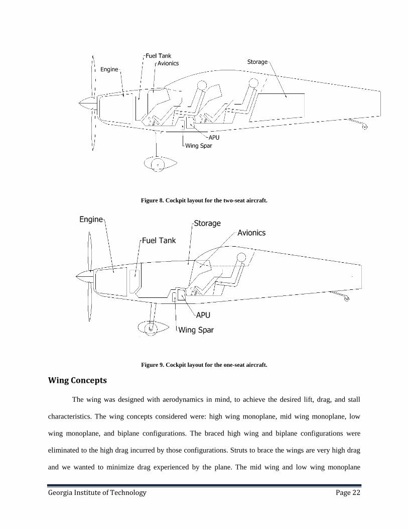
The dimensions of the fuselage were selected based on data gathered from similar aircraft and
based on the space needed to accommodate a range of pilot sizes in the cockpit layout. The length of the
fuselage was selected as 19.7 ft and the width was selected as 2.7 ft, yielding a fineness ratio of 7.3. This
is illustrated below in Figure 7. The cockpit layouts for the two-seat and one-seat members of the CARL
family are shown below in Figure 8 and Figure 9, respectively. The pilots shown in the figures are 6’2”
tall, and the rudder pedals are adjustable to accommodate a range of pilot heights. As shown in the figures
below, the one-seat aircraft is nearly the same as the two-seat in the fuselage, but the front seat is removed
and a fuselage plug and smaller canopy are installed. By keeping so much of the structure the same,
manufacturing costs are lowered.
Figure 7. Fuselage dimensions for the two-seat CARL aircraft.
Georgia Institute of Technology Page 22
Figure 8. Cockpit layout for the two-seat aircraft.
Figure 9. Cockpit layout for the one-seat aircraft.
Wing Concepts
The wing was designed with aerodynamics in mind, to achieve the desired lift, drag, and stall
characteristics. The wing concepts considered were: high wing monoplane, mid wing monoplane, low
wing monoplane, and biplane configurations. The braced high wing and biplane configurations were
eliminated to the high drag incurred by those configurations. Struts to brace the wings are very high drag
and we wanted to minimize drag experienced by the plane. The mid wing and low wing monoplane
Georgia Institute of Technology Page 23
designs both had the advantage of making entry and exit into the airplane easy by stepping onto the wing
and climbing into the cockpit, but the mid wing presented the problem of placing the wing spar so it did
not run through the cockpit and interfere with the cockpit layout. The low wing avoided that problem and
thus a low wing monoplane wing configuration was selected. With the wing configuration selected, the
airfoil, taper ratio, sweep angle, and other wing parameters had to be selected.
The aerodynamics of CARL are tailored for a combination of aerobatic effectiveness and
aerodynamic efficiency. While the latter is achieved with drag minimization in mind for each component
of the aircraft, the former is a more localized problem. The first consideration made is to select a good
airfoil for aerobatics. Characteristics of good aerobatic airfoils include 10-16% thickness, a small leading
edge radius, a symmetric design for inverted flight, and sudden stall characteristics to give pilots more
control during maneuvers. As a secondary consideration, a thicker airfoil also results in a lighter wing due
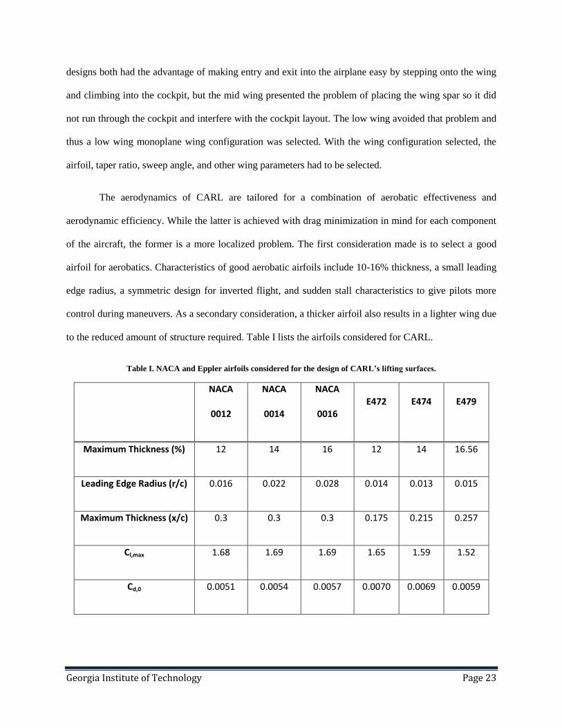
to the reduced amount of structure required. Table I lists the airfoils considered for CARL.
Table I. NACA and Eppler airfoils considered for the design of CARL’s lifting surfaces.
NACA
0012
NACA
0014
NACA
0016 E472 E474 E479
Maximum Thickness (%) 12 14 16 12 14 16.56
Leading Edge Radius (r/c) 0.016 0.022 0.028 0.014 0.013 0.015
Maximum Thickness (x/c) 0.3 0.3 0.3 0.175 0.215 0.257
Cl,max 1.68 1.69 1.69 1.65 1.59 1.52
Cd,0 0.0051 0.0054 0.0057 0.0070 0.0069 0.0059

Georgia Institute of Technology Page 24
Using XFOIL, the airfoils are analyzed in viscous flow at a Reynold’s number of four million,
similar to what the aircraft is expected to encounter in flight. Figure 10 shows a plot of airfoil lift
coefficient vs. angle of attack. It is clear from the plot that the Eppler airfoils, especially the E472 and
E474, have much more sudden stalls than the NACA airfoils, demonstrating their effectiveness for
aerobatic flight. However, there is also a noticeable penalty in the maximum lift coefficient of the Eppler
airfoils.
Figure 10. Sectional lift coefficient vs. angle of attack for the airfoils considered for CARL.
To compare aerodynamic efficiency of the airfoils, Figure 11 shows a plot of lift to drag ratio vs.
sectional lift coefficient for each airfoil. In the plot, larger “spirals” indicate that the airfoil is more
efficient for a given lift coefficient. Intuitively, the E472 is much more efficient than the other Eppler
airfoils due to its reduced thickness, making it appear to be an attractive choice for the design airfoil.
However, a thinner airfoil also generally leads to a heavier wing structure. Because of the importance of
weight in the design of this aircraft and the reasonable effectiveness of the E474, the E474 is selected as
the airfoil of choice for this aircraft.
0
0.2
0.4
0.6
0.8
1
1.2
1.4
1.6
1.8
0 5 10 15 20 25 30
Lift
Co
effi
cien
t (C
l)
Angle of Attack (degrees)
NACA 0012
NACA 0014
NACA 0016
E479
E472
E474

Georgia Institute of Technology Page 25
Figure 11. Lift to drag ratio vs. sectional lift coefficient for the airfoils considered for CARL.
Figure 12 shows a plot of the geometry of the Eppler 474. Note that the location of maximum
thickness of the airfoil is relatively far forward, which produces the sudden stall effect, but tends to lead
to more drag for the aircraft.
Figure 12. Geometry of the Eppler 474.
0
20
40
60
80
100
120
140
0 0.5 1 1.5 2
Lift
to
Dra
g R
atio
Lift Coefficient (Cl)
NACA 0012
NACA 0014
NACA 0016
E479
E472
E474
-0.3
-0.2
-0.1
0
0.1
0.2
0.3
0 0.2 0.4 0.6 0.8 1
Georgia Institute of Technology Page 26
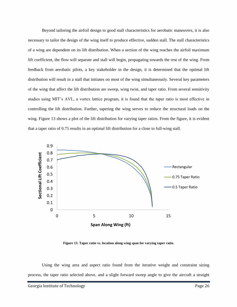
Beyond tailoring the airfoil design to good stall characteristics for aerobatic maneuvers, it is also
necessary to tailor the design of the wing itself to produce effective, sudden stall. The stall characteristics
of a wing are dependent on its lift distribution. When a section of the wing reaches the airfoil maximum
lift coefficient, the flow will separate and stall will begin, propagating towards the rest of the wing. From
feedback from aerobatic pilots, a key stakeholder in the design, it is determined that the optimal lift
distribution will result in a stall that initiates on most of the wing simultaneously. Several key parameters
of the wing that affect the lift distribution are sweep, wing twist, and taper ratio. From several sensitivity
studies using MIT’s AVL, a vortex lattice program, it is found that the taper ratio is most effective in
controlling the lift distribution. Further, tapering the wing serves to reduce the structural loads on the
wing. Figure 13 shows a plot of the lift distribution for varying taper ratios. From the figure, it is evident
that a taper ratio of 0.75 results in an optimal lift distribution for a close to full-wing stall.
Figure 13. Taper ratio vs. location along wing span for varying taper ratio.
Using the wing area and aspect ratio found from the iterative weight and constraint sizing
process, the taper ratio selected above, and a slight forward sweep angle to give the aircraft a straight
0
0.1
0.2
0.3
0.4
0.5
0.6
0.7
0.8
0.9
0 5 10 15
Sect
ion
al L
ift
Co
effi
cien
t
Span Along Wing (ft)
Rectangular
0.75 Taper Ratio
0.5 Taper Ratio

Georgia Institute of Technology Page 27
leading edge, the planform geometry of the wing is specified in Table II. Note that the slight forward
sweep biases the lift distribution very slightly towards that of the rectangular wing, but the sweep angle is
small enough such that its effect on the lift distribution is approximately negligible. Due to the
commonality of empty weight requirements, the wing design is the same between the single and two seat
variants. From AVL, the maximum lift coefficient of the aircraft with this wing design is 1.45.
Table II. Wing planform geometry.
Specification Value
Area (ft2) 131
Aspect Ratio 5.5
Span (ft) 26.8
Sweep (deg) -1.5
Taper Ratio 0.75
Root Chord (ft) 5.6
Tip Chord (ft) 4.2
Thickness to Chord (t/c) 0.14
Incidence Angle (deg) 0
Dihedral Angle (deg) 0
Airfoil E474

Georgia Institute of Technology Page 28
Tail Concepts
The tail concepts considered include a conventional tail, a T-tail, and a V-tail. While the T-tail is
a good choice if a conventional tail would be in the messy airflow coming from engine exhaust, it
requires increased structural weight in the vertical tail to put the horizontal tail at the top. For a design
with a propeller at the front, there would be no substantial benefit to using a T-tail, but the structural
weight penalty would make it difficult to meet the light-sport weight requirements. A V-tail was also
considered, primarily for aesthetics, but the complexity of both the structure and the control system
outweigh the benefits of aesthetics, as once again there is no need to use anything other than a
conventional tail for aerodynamic reasons. Thus, a conventional tail was selected.
Tail sizing was performed to ensure adequate stability of the aircraft and is detailed below in the
Tail Sizing section.
Propulsion System
The design of the propulsion system was broken into two parts, the engine and the propeller. The
first step was choosing an engine that could provide at least the power dictated by the constraint sizing
without having too much excess power and passing the speed limit. For this task, the Rotax 915S was
selected. This Rotax engine provides the necessary power, with the additional advantage of being very
light. In such a small aircraft, even a light engine constitutes a significant portion of the weight. Thus
saving weight in the engine has a large impact on the weight of the aircraft. The Rotax 915S is scheduled
to be in production by late 2017, well before the aircraft would be expected to begin production in 2020.
Two specific pieces of equipment will be installed and connected to the engine to ensure that the
engine is capable of providing the required performance. The first is a pump on the fuel tanks. This pump
ensures that during inverted flight, there is constant fuel flow into the engine. The second is a RPM
limiter. This device reads the RPM of the engine and limits the fuel flow into the engine when it
approaches its maximum sustainable RPM. Without this device, the engine could be burned out by a

Georgia Institute of Technology Page 29
strong gust of wind, dive, or similar form of acceleration that causes the propeller to accelerate past a safe
rate of rotation.
With an engine in place, a propeller was designed using the predicted engine data. The main goal
of the propeller design was to provide maximum cruise efficiency while limiting the maximum speed in
steady level flight to less than 120 knots. The propeller design was performed in the computer program
XRotor. XRotor used the design parameters listed in Table III to create propeller geometry. This
geometry could then be analyzed, in conjunction with the predicted engine performance, at off-design
points.
Table III. XRotor Design Parameters
Parameter Value
Number of Blades 2
Propeller Radius (in) 37.4
Hub Radius (in) 3.94
Hub Wake Radius (in) 1.97
Airspeed (knots) 100
Propeller RPM 2,262
Power (Hp) 125
Lift Coefficient 0.45
Most aerobatic light sport aircraft have either two or three balded propellers. A two blade design
was chosen for this aircraft to keep the propulsive efficiency higher. Anderson’s text Vehicle
Performance and Design [2] provides a useful approximation for the propeller radius based on the power
of the engine. This radius is not large enough to cause the propeller tips to exceed Mach 1 at maximum
speed, which is a common issue for aircraft with two propellers. The size of the hub radius and wake
radius were taken as average values from the geometry of this and other similar light sport aircraft. The
values of the propeller RPM and power came directly from interpolations done on engine performance
data provided by Rotax.

Georgia Institute of Technology Page 30
The propeller blade geometry was very sensitive to the final two design parameters, airspeed and
propeller lift coefficient. For this reason, the design process was repeated for various values of each so
that the final values would be known to produce the most efficient propulsive performance. Figure 14
shows how the thrust available curve changes as the propeller geometry is designed at various lift
coefficients. It is clear that a higher lift coefficient results in a maximum speed greater than the imposed
limit of 120 knots. By simple visual inspection, it would appear that the lift coefficients of 0.35 and 0.45
yield almost identical performance. However, the propeller blade designed with a lift coefficient of 0.35
has much worse propulsive efficiency at speeds greater than 100 knots. Since efficient cruise is of high
priority, the lift coefficient was decided to be 0.45.
Figure 14. Thrust Available for Various Propeller CL
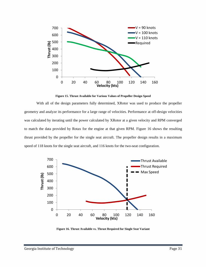
The second design parameter studied was the design velocity. Figure 15 shows how a higher
design velocity sacrifices low speed thrust in order to retain more thrust at higher speeds. In terms of this
tradeoff, a design velocity of 100 knots provided the best balance. Higher design velocities resulted in
maximum speeds that were higher than allowable. Lower design velocities became either inefficient at
cruise speed, or unable to break 100 knots at all.
0
100
200
300
400
500
600
700
0 20 40 60 80 100 120 140 160
Thru
st (
lb)
Velocity (kts)
CL=0.35
CL=0.45
CL=0.6
Required
Georgia Institute of Technology Page 31
Figure 15. Thrust Available for Various Values of Propeller Design Speed
With all of the design parameters fully determined, XRotor was used to produce the propeller
geometry and analyze its performance for a large range of velocities. Performance at off-design velocities
was calculated by iterating until the power calculated by XRotor at a given velocity and RPM converged
to match the data provided by Rotax for the engine at that given RPM. Figure 16 shows the resulting
thrust provided by the propeller for the single seat aircraft. The propeller design results in a maximum
speed of 118 knots for the single seat aircraft, and 116 knots for the two-seat configuration.
Figure 16. Thrust Available vs. Thrust Required for Single Seat Variant
0
100
200
300
400
500
600
700
0 20 40 60 80 100 120 140 160
Thru
st (
lb)
Velocity (kts)
V = 90 knots
V = 100 knots
V = 110 knots
Required
0
100
200
300
400
500
600
700
0 20 40 60 80 100 120 140 160
Thru
st (
lb)
Velocity (kts)
Thrust Available
Thrust Required
Max Speed

Georgia Institute of Technology Page 32
Landing Gear Design
The decision of the landing gear configuration was between conventional (taildragger) and
tricycle. The former was ultimately chosen for the following reasons. Due to its position further from the
center of gravity, the tailwheel supports a smaller portion of the aircraft’s weight, allowing it to be much
smaller and lighter than a nose wheel. Weight reduction was key for this aircraft with the LSA weight
limit. As a result of the tailwheel being smaller, parasitic drag is also reduced and consequently the
aerodynamic performance is improved. The propeller has much more clearance due the orientation of the
aircraft which will protect it from chip damage when landing on rough or gravel airstrips. There are some
disadvantages to the conventional configuration, however. The angled disposition of the aircraft reduces
the visibility of the pilot making taxiing more difficult. The taildragger configuration is also sensitive to
high wind conditions when taxiing because of the high angle of attack on the wings, making handling
much more difficult. It is also more susceptible to ground looping, or sudden loss of directional controls
which can result in damages to the wing, fuselage, tires, or propeller. The performance and weight
benefits of the conventional design overshadowed its physical inconveniences.
The detailed design of the landing gear after the landing gear configuration was selected is shown
below in the Landing Gear section.
Three-View
With the configuration selected and the fuselage, wing, tail, and landing gear designed, a 3-
dimensional model of the aircraft was created to use in further analysis. The design resulting from the
configuration decisions outlined in the previous sections is shown below. The one-seat CARL aircraft is
shown in Figure 17 and the two-seat aircraft is shown in Figure 18. Both figures include the aircraft C.G.
and aerodynamic center as well as the aerodynamic centers of the vertical and horizontal tails.

Georgia Institute of Technology Page 33
Figure 17. Three-view of the 3-d model of the one-seat CARL aircraft including C.G. information.
Figure 18. Three-view of the 3-d model of the two-seat CARL aircraft including C.G. information.

Georgia Institute of Technology Page 34
Performance
The following performance parameters will be discussed in this chapter:
Aerodynamics
Takeoff and Landing
Range
Rate of Climb
V-n Diagram
Aerodynamics
From the wing geometry shown above in the Wing Concepts section and the aircraft geometry
broken down throughout this report, a Class II drag polar of the aircraft is created. This drag polar is
formulated using methodology specified in Roskam Part VI [18] and Hoerner’s “Fluid Dynamic Drag
[10] .” To summarize, for each component of the aircraft, the parasite drag and the drag due to lift are
determined using a mix of empirical relations and basic aerodynamic equations. The drag of each
component is then normalized by the ratio between its wetted area and the reference area of the wing.
Figure 19 shows charts of the parasite drag contribution for each component of the drag of each aircraft.
Note that these charts are produced for trimmed flight during the aircraft cruise condition, or 7000 feet at
110 knots CAS.
Figure 19. Parasite drag breakdown for the single and two seat variations of CARL.
Single Seat Aircraft Two Seat Aircraft
Wing
Fuselage
Horizontal Tail
Vertical Tail
Landing Gear
Canopy
Trim
Interference

Georgia Institute of Technology Page 35
From the figures, it is clear that the wing dominates the zero lift drag, closely followed by the
fuselage and landing gear. This makes sense because the wing has the largest wetted area of any
component at 262 ft2, with the fuselage behind at 153 ft
2. The fixed landing gear, on the other hand, while
not a large component of wetted area, produces a large portion of the drag due to its irregular shape, even
with fairings covering the wheels. Because geometrically, the only difference between the two airplanes is
the canopy, it makes sense that the biggest difference between the two pie charts is in the relative
magnitude of the canopy drag.
Figure 20 shows the Class II drag polar of the two seat aircraft compared to the Class I drag polar
used in the initial sizing process. It is clear that the Class II drag polar is very close to the Class I results
used in the initial weight and constraint sizing, increasing the confidence in the drag analysis and the
specification of the aircraft geometry.
Figure 20. Comparison of Class II drag polar with Class I results.
The Class II drag results are then used to determine the lift to drag ratio for the cruise and reserve
missions of the aircraft and to determine the thrust required to maintain steady level flight at different
velocities. The former is important to determining the cruise performance of the aircraft, while the latter is
0
0.2
0.4
0.6
0.8
1
1.2
1.4
1.6
0 0.02 0.04 0.06 0.08 0.1 0.12 0.14 0.16 0.18
Lift
Co
effi
cien
t (C
L)
Drag Coefficient (CD)
Class I
Class II

Georgia Institute of Technology Page 36
important in designing the propulsion system so as not to exceed the maximum LSA speed of 120 knots.
Table IV summarizes the lift to drag ratios for each aircraft for the cruise and endurance missions, and the
thrust required curve is shown in Figure 14 in the Propulsion section of this report.
Table IV. Lift and drag parameters during the cruise and reserve missions for CARL.
Two Seat One Seat
CD,0 0.0236 0.0237
CL,cruise 0.295 0.261
CL,reserve 0.277 0.245
L/Dcruise 10.2 9.3
L/Dreserve 9.7 9.0
Takeoff and Landing
Takeoff and landing lengths were calculated using the standard force based approach given in
Anderson’s Aircraft Performance and Design [2]. The takeoff length accounts for both the ground roll
and airborne segments, and the landing length includes the approach, flare, free roll, and ground roll
segments. As required by the RFP, the takeoff and landing lengths necessary for the aircraft to clear a 50
ft obstacle are shown for the following conditions:
1. Dry Pavement Runway, Sea Level ISA +10°C
2. Dry Pavement Runway, 5000 ft ISA +10°C
3. Grass Field, Sea Level ISA +0°C

Georgia Institute of Technology Page 37
The RFP stipulates that both the takeoff and landing lengths at Condition 1 be less than 1200 ft
for the single seat variant and less than 1500 ft for the two seat variant. The takeoff performance of the
single and two seat variants is shown in Figure 21 and Figure 22, respectively.
Figure 21. Single Seat Variant Takeoff Performance
Figure 22. Two Seat Variant Takeoff Performance
0 500 1000 1500
RFP Requirement
Pavement 5000 ft, +10 °C
Pavement Sea Level, +10 °C
Grass Sea Level, +0 °C
Takeoff Distance (ft)
0 500 1000 1500 2000
RFP Requirement
Pavement 5000 ft, +10 °C
Pavement Sea Level, +10 °C
Grass Sea Level, +0 °C
Takeoff Distance (ft)

Georgia Institute of Technology Page 38
The aircraft’s powerful engine allows both variants to easily surpass the required takeoff
performance: the single seat variant requires fewer than 475 ft and the two seat variant requires fewer
than 535 ft to land at Condition 1. Additionally, the low takeoff lengths exhibited by the aircraft at
nonstandard conditions indicate that both variants can provide superior takeoff performance in a variety
of potential flight scenarios. The landing performance of the single and two seat variants is shown in
Figure 23 and Figure 24, respectively.
Figure 23. Single Seat Variant Landing Performance
Figure 24. Two Seat Variant Landing Performance
950 1000 1050 1100 1150 1200 1250
RFP Requirement
Grass Sea Level, +0 °C
Pavement 5000 ft, +10 °C
Pavement Sea Level, +10 °C
Landing Distance (ft)
0 500 1000 1500 2000
RFP Requirement
Grass Sea Level, +0 °C
Pavement 5000 ft, +10 °C
Pavement Sea Level, +10 °C
Landing Distance (ft)

Georgia Institute of Technology Page 39
The single seat and two seat variants require 1035 ft and 1070 ft, respectively, to land at
Condition 1. The landing performance therefore exceeds the requirements given by the RFP. In fact, even
on a grass landing field, the single and two seat variants can achieve the RFP maximum landing distances
required for dry pavement. This added versatility provides pilots the option to safely land in suboptimal
conditions.
Range
The RFP dictates that the single seat variant have a cruise range of at least 300 nm and that the
two seat variant have a cruise range of at least 250 nm. Aircraft cruise range was determined with the
method outlined in Roskam’s Airplane Design for a propeller driven aircraft. Figure 25 and Figure 26
show the payload-range diagrams of the single and two seat variants, respectively. The maximum fuel
weight constitutes the replacement of 15 lb of payload with 15 lb of additional fuel, and the minimum
payload constitutes the maximum fuel weight and only the payload necessary for safe operation of the
aircraft. It is important to note that the minimum payload of the two seat variant includes only one pilot.
Figure 25. Single Seat Variant Payload-Range
245
250
255
260
265
270
275
280
0 100 200 300 400 500
Payl
oad
(lb
)
Range (nm)
Max Payload

Georgia Institute of Technology Page 40
Figure 26. Two Seat Variant Payload Range
As shown in the payload-range diagrams, each variant meets its required cruise range when fully
loaded. Additionally, both aircraft can be flown for much further cruise distances if the maximum fuel
weight and minimum payload weights are used.
Rate of Climb
The aircraft climb rate is approximated as the excess specific power at the optimal climb speed.
Calculation of this value is detailed in the Propulsion System section of the report. The RFP requires that
the climb rate be at least 1500 fpm for the single seat variant and at least 800 fpm for the two seat variant.
Figure 27 compares the actual aircraft climb rates to these requirements.
215
265
315
365
415
465
515
0 100 200 300 400 500
Payl
oad
(lb
)
Range (nm)
Max Payload Max Fuel
Min Payload

Georgia Institute of Technology Page 41
Figure 27. Single and Two Seat Variant Climb Rates
As is clearly shown, both variants far exceed their required climb rates: the single seat climbs at a
rate of 3400 fpm and the two seat climbs at a rate of 2650 fpm. These values increase the aircraft’s ability
to compete in aerobatic competitions, as many maneuvers are enhanced by strong climb performance.
V-n Diagram
The V-n diagrams of the required performance envelopes of the CARL aircraft were created to
illustrate the loads the aircraft must withstand. The V-n diagram for the one-seat aircraft is shown in
Figure 28 and the V-n diagram for the two-seat aircraft is shown in Figure 29. The one-seat aircraft must
stand maneuvering loads of +6/-5 G and the two-seat must withstand +6/-3. Both aircraft should be able
to withstand gusts of +/- 50 fps at cruise and +/- 25 fps at dive speed. The dive speed for each aircraft was
designed to be 1.55 times the cruise speed, which led to a dive speed of 170.5 kts, or 288 fps. Cruise
speed is labeled on the diagrams at 110 kts, or 186 fps. From both diagrams it is clear that the gust loads
lie within the maneuvering portion of the diagram and that the maneuvering loads should be analyzed to
ensure the structural ability of the aircraft to perform within the required envelope. The structural strength
of the aircraft is detailed more below in the Structure and Manufacturing section.
0 1000 2000 3000 4000
Single Seat
Two Seat
Climb Rate (ft/min)
Required Actual

Georgia Institute of Technology Page 42
Figure 28. V-n diagram showing loads required of the one-seat CARL aircraft.
Figure 29. V-n diagram showing loads required of the two-seat CARL aircraft.

Georgia Institute of Technology Page 43
Weight and Balance
In this section, the weight and balance of the CARL aircraft is presented and discussed. The
analysis and modeling methods will be discussed, and the results tabulated and presented graphically.
Class II component weight estimates for both variations are offered, as well as center of gravity locations
in the form of excursion diagrams.
Class II Weight and Balance
The methodology used to analyze the class II weight and balance of the aircraft is that laid out in
Part V of Roskam’s Airplane Design series [18]. Initially, a gross take-off weight and empty weight were
assumed based on the provided RFP and regression data from two dozen aircraft of similar size and
mission profile. From this base line, and “Cessna” component weight estimation equations in Airplane
design Part V as well as equation in Torenbeek’s Synthesis of Subsonic Airplane Design, a detailed
component and group based weight statement was built up [22]. As the design process progressed, more
accurate weight information was incorporated into the statements.
In Table V below, a weight statement is provided for the two-seat member of the CARL family.
The weight is divided into groups and subdivided into smaller components. In the bottom right of this
table the gross take-off weight and empty weights are also stated.

Georgia Institute of Technology Page 44
Table V. Two-seat CARL aircraft component weight statement.
Structure Removable
Component % lb Component % lb
Wing 13.7 173.7 Pilots 31.5 400.0
Horizontal Tail 1.6 20.0 Fuel 5.5 69.7
Vertical Tail 0.9 11.8 Baggage 2.4 30.0
Fuselage 7.6 96.0 Safety System 2.4 30.0
Landing Gear 5.5 69.6 Ballast 0.8 10.0
Power Plant Fixed Equipment
Component % lb Component % lb
Engine 14.6 185.0 Avionics + Instrumentation 2.1 26.7
Fuel System 1.2 14.7 Flight Control 1.7 21.3
Propeller 2.3 29.2 Furnishing 1.8 23.4
Auxiliary Power 1.3 16.5
Group Totals Smoke System 3.2 40.5
Group % lb
Structure 29.3 371.0
Removable 42.6 539.7 Gross Take-off Weight 1268 lb
Fixed Equipment 10.1 128.4 Empty Weight 728 lb
Power Plant 18.0 228.8
It can be seen from the gross take-off weight that this variant is well within the maximum take-off
weight cap of 1320 lb set by the FAA’s definition of LSA. In Table VI below, a weight statement is
similarly provided for the one-seat member of the CARL family.

Georgia Institute of Technology Page 45
Table VI. Two-seat CARL aircraft component weight statement.
Structure Removable
Component % lb Component % lb
Wing 16.7 173.7 Pilots 22.1 230.0
Horizontal Tail 1.9 20.0 Fuel 6.2 64.9
Vertical Tail 1.1 11.8 Baggage 2.9 30.0
Fuselage 9.2 96.0 Safety System 1.4 15.0
Landing Gear 6.7 69.6 Ballast 0.4 5.1
Power Plant Fixed Equipment
Component % lb Component % lb
Engine 17.8 185.0 Avionics + Instrumentation 1.7 18.1
Fuel System 1.4 14.7 Flight Control 1.7 17.5
Propeller 2.8 29.2 Furnishing 1.0 10.1
Auxiliary Power 1.0 10.7
Group Totals Smoke System 3.9 40.5
Group % lb
Structure 35.6 371.1
Removable 31.6 345.0 Gross Take-off Weight 1041 lb
Fixed Equipment 10.8 96.9 Empty Weight 697 lb
Power Plant 22.0 228.9
This member of the CARL family is just over 200 pounds lighter than its two-seat counter-part
when fully loaded. Component weights for pilots, baggage, and safety systems (parachutes) are exactly
those stated in the RPF. Several of the other component weights such as fuel and avionics did not come
from equations, but were instead derived based on other information at our disposal. The fuel weight is
selected to meet the RPF requirements for range, as shown in the preceding performance section, and
avionics weight is established from a detailed inventory of avionics and other electrical and
instrumentation components incorporated into the aircrafts subsystems. The precise weight breakdown of
avionics is withheld from this section to be presented as a part of a more complete conception in the
subsystems section.
The following figures illustrate the proportional weights of each component, and an attempt was
made to help visualize the proportional weights of groups as well through color schemes. It is made

Georgia Institute of Technology Page 46
apparent from comparing the two figures that the absence of one pilot in the one-seat variant is the chief
reason for the weight dissimilarity.
Figure 30. Two-seat component and group proportional weight visualization.
Wing Horizontal Tail Vertical Tail Fuselage Landing Gear Engine Fuel System Propeller Avionics + Instrumentation Flight Control Furnishing Auxiliary Power Pilot Fuel Baggage

Georgia Institute of Technology Page 47
Figure 31. One-seat component and group proportional weight visualization.
One major sacrifice in terms of weight came from integrating the weight of the smoke system.
Though not essential, it would be a nice touch for amateur and experienced aerobatic pilots alike.
Because this component was so heavy and voluminous, it would be unreasonable to simply list it as an
optional part of the plane without making an allowance for it in the component placement phase, weight
statement, and performance analysis. Another important note about the weight is the relatively small
ballasts incorporated in both the one and two seat variants with a slightly larger ballast listed for the two
seat. The importance of this component will be discussed in detail in the following center of gravity
excursion section. As mentioned in the engine discussion previously, the selected engine is not yet
available on the market, and as such, the weight listed on the manufacturers website is an estimate subject
to amendment. This estimate was used in the weight statement since this is a better source than an
equation attempting to correlate horsepower and weight.
A requirement for this aircraft is a commonality of 75% of the empty weight between the two
variants, not including the engine and propeller. The most conservative interpretation of this requirement
Wing Horizontal Tail Vertical Tail Fuselage Landing Gear Engine Fuel System Propeller Avionics + Instrumentation Flight Control Furnishing Auxiliary Power Pilot Fuel Baggage

Georgia Institute of Technology Page 48
would mean that 75% of the empty weight of the one-seater, not including the engine and propeller, (362
lb), should be re-used in the two-seat variant. In order to realize this, almost the entire structural weight is
to be reused. Although the actual listed weights are identical, the treatment of this structural weight for
the fuselage will differ since the canopy is altered. One advantage of keeping so much commonality
between the structures is that the one-seat variant would be able handle higher g loads than the RPF
necessitates. This is desirable since this variant is meant to be more competitive than its two-seat
counterpart. The structural commonality accounts for around 330 lb of common weight, and the smoke
system alone covers the remaining 32 lb required. Beyond that, the one-seat furnishing weight is
completely re-used, along with much of its avionics, instrumentation, and flight controls.
CG Excursion Diagram
Utilizing the component weights and locations described above, C.G. excursion diagrams were
created. The component relative masses and centers of gravity were found and used to systematically
map the aircrafts center of gravity for a range of loaded and unloaded configurations.
The matrices in Table VII and Table VIII demonstrate the systematic approach used to observe
the motion of the center of gravity (C.G.). In addition to the conditions defined in these matrices, the
forward most C.G. location found from this process was re-tested minus the pilot.
Table VII. One-seat C.G. excursion tested configurations.
1 2 3 4
Fuel
No Fuel
Baggage
No Baggage

Georgia Institute of Technology Page 49
Table VIII. Two-seat C.G. excursion tested configurations.
1 2 3 4 5 6 7 8 9 10 11 12
Fuel
No Fuel
Baggage
No Baggage
Two Pilots
One Pilot (back)
One Pilot (front)
In Figure 32, the locations where component masses are centered for the one-seat variant are
shown.
Figure 32. Component weight locations in the one-seat CARL aircraft.
The outcomes of this analysis are shown most effectively in C.G. excursion diagrams. Figure 33
shows the C.G. excursion diagram for the one-seat variant in addition to a line showing a longitudinal tip
over margin set back 15 degrees from where tip over would begin to take place with the aircraft at rest on
the ground. The dimensions specified in the figures are relative to a point 24 inches in front of the
fuselage tip and 24 inches below the bottommost point on the wheel. The dimensions apply to the aircraft
oriented as displayed in Figure 32.

Georgia Institute of Technology Page 50
Figure 33. C.G. excursion diagram for the one-seat CARL aircraft.
In Figure 34, the C.G. movement for the two-seat variant is shown. It can be seen that the major
factor that affects the C.C. location is the loading and unloading of the pilots. Because this only occurs on
the ground, the handling qualities associated with the static margin will remain fairly constant throughout
any single flight.
Figure 34. C.G. excursion diagram for the two-seat CARL aircraft.
67
68
69
70
71
72
73
78 83 88 93 98 103
C.G
. Z lo
cati
on
(in
)
C.G. X location (in)
unload fuel
unload baggage
load fuel
load baggage
Pilot Loading
Longitudinal Tip Over
67.2
67.4
67.6
67.8
68
68.2
68.4
68.6
68.8
69
78 83 88 93 98 103
C.G
. Z lo
cati
on
(in
)
C.G. X location (in)
unload fuel
load baggage
load fuel
unload baggage
Two Pilots
One Pilot in Back Seat
One Pilot in Front Seat

Georgia Institute of Technology Page 51
From inspecting both excursion diagrams, it is clear that the outlier for possible flight conditions
is the case when the two-seat variant is flown from the front seat. Although even in this condition, the
aircraft is still flyable and stable within the built in margins, it is still advised that a single pilot flying the
two seat aircraft do so from the back seat.
As mentioned in the class II weight and balance section, there is a noncompulsory ballast for this
aircraft (5 lb for the one-seat, and 10 lb for the two-seat). The C.G. excursion diagrams were made
assuming the ballast weight to be at the overall C.G., so it did not affect the excursion excepting to
negligibly weight the aircraft at its C.G., and thus diminish the effect of moving other weights. Without
the ballasts, the aircraft has no stability, balance, or tip over problems. However, it was mentioned in a
survey of aerobatic pilots conducted by ASDL at the Georgia Institute of Technology, that the capacity to
fine-tune the static margin would be highly desirable. With these ballasts, the pilot could either make the
controls more amenable to longer flights near steady cruise conditions, or lessen the stability to make
aerobatic maneuvers easier and quicker to perform simply by relocating a weight to one of several
stations that it can fastened to.
Landing Gear
With the landing gear configuration selected, the next step is to place the nose gear and
tailwheel. The two nose wheels will be placed 50.5 inches from the front of the fuselage. This places them
in front of the wing. Figure 35 displays the locations of the landing gear relative to the aircraft C.G. The
variant shown in this figure is the two-seat aircraft. The gear was designed around this configuration
because it experiences a more forward C.G. than the one-seat aircraft. The tailwheel is placed 178 inches
from the front of the fuselage. The aircraft will sit at an angle of 10 , allowing it to successfully take off
without a tail strike incident.
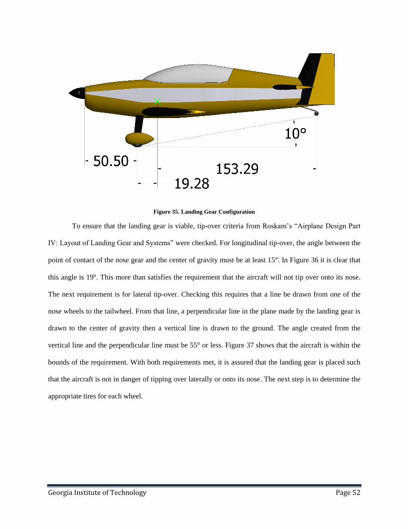
Georgia Institute of Technology Page 52
Figure 35. Landing Gear Configuration
To ensure that the landing gear is viable, tip-over criteria from Roskam’s “Airplane Design Part
IV: Layout of Landing Gear and Systems” were checked. For longitudinal tip-over, the angle between the
point of contact of the nose gear and the center of gravity must be at least 15 . In Figure 36 it is clear that
this angle is 19 . This more than satisfies the requirement that the aircraft will not tip over onto its nose.
The next requirement is for lateral tip-over. Checking this requires that a line be drawn from one of the
nose wheels to the tailwheel. From that line, a perpendicular line in the plane made by the landing gear is
drawn to the center of gravity then a vertical line is drawn to the ground. The angle created from the
vertical line and the perpendicular line must be 55 or less. Figure 37 shows that the aircraft is within the
bounds of the requirement. With both requirements met, it is assured that the landing gear is placed such
that the aircraft is not in danger of tipping over laterally or onto its nose. The next step is to determine the
appropriate tires for each wheel.

Georgia Institute of Technology Page 53
Figure 36. Longitudinal tip-over criterion showing that the aircraft will not tip over.

Georgia Institute of Technology Page 54
Figure 37. Lateral tip-over criterion verifying the landing gear placement.
In order to select the tires, the loads placed on each strut must first be determined. Figure 35 gives
the length of landing gear with respect to the center of gravity. The static loads for the landing gear are
determined by the following equations.
(1)
(2)

Georgia Institute of Technology Page 55
Equation 1 is for the loading on the nose gear and Equation 2 is for the tailwheel. The take-off
weight is 1268 lb. The distance from the center of gravity to the nose, , and tail gear, , is 19.28 and
152.98 inches, respectively. Therefore the static load per nose wheel is 563 lb and for the tail is 147 lb.
Next, the dynamic load per nose gear must be calculated using the following equation.
(3)
In Equation 3,
is the brake factor and for this case 0.4 will be used based on historical data.
The dynamic load per nose gear is calculated to be 625 lb. The final piece needed for the tire requirements
is tire operating speed. For landing this is simply 1.2 times the landing speed which is 70 kts. For takeoff
it is 1.1 times the takeoff velocity which is 59.4 kts. From the values of operating speeds and loads, the
Goodyear Flight Custom III 7.00-6-6 was chosen. This tire is integrated with Kevlar so it is more resilient
to rough runways and thus can have a longer lifespan. It also has wide aquachannel grooves for improved
wet traction. The tailwheel tire was selected to be an Alaskan Bushwheel 3200.
A dimensioned drawing of the nose gear is shown in Figure 38. Wheel fairings are used to create
smooth laminar flow over the wheel, avoiding the turbulent flow a fully exposed wheel might experience.
They also prevent mud and gravel being thrown up from damaging the fuselage, wing and propeller.

Georgia Institute of Technology Page 56
Figure 38. Dimensioned models of the CARL nose gear.
Structure and Manufacturing
This chapter documents the selection of materials for the wings, fuselage, empennage, and
landing gear, as well as the general structural layout of the primary airframe structure.
Materials Selection
The main groups for which materials selection was considered are: fuselage, tail, wings, and
landing gear. It was considered to manufacture the bulk of the vehicle out of composite materials to save
weight and boost performance, but in light of several recent catastrophic failures of all-composite
aerobatic aircraft and with the difficulty detecting defects from fatigue on composite structures, it was
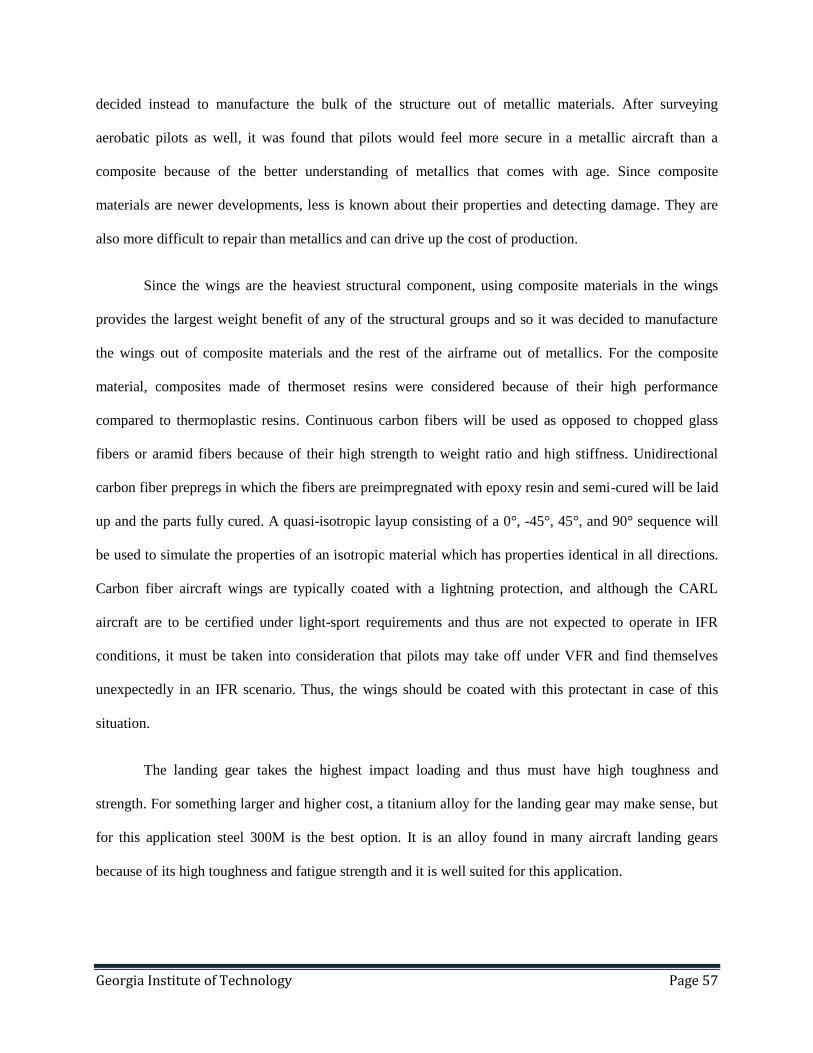
Georgia Institute of Technology Page 57
decided instead to manufacture the bulk of the structure out of metallic materials. After surveying
aerobatic pilots as well, it was found that pilots would feel more secure in a metallic aircraft than a
composite because of the better understanding of metallics that comes with age. Since composite
materials are newer developments, less is known about their properties and detecting damage. They are
also more difficult to repair than metallics and can drive up the cost of production.
Since the wings are the heaviest structural component, using composite materials in the wings
provides the largest weight benefit of any of the structural groups and so it was decided to manufacture
the wings out of composite materials and the rest of the airframe out of metallics. For the composite
material, composites made of thermoset resins were considered because of their high performance
compared to thermoplastic resins. Continuous carbon fibers will be used as opposed to chopped glass
fibers or aramid fibers because of their high strength to weight ratio and high stiffness. Unidirectional
carbon fiber prepregs in which the fibers are preimpregnated with epoxy resin and semi-cured will be laid
up and the parts fully cured. A quasi-isotropic layup consisting of a 0°, -45°, 45°, and 90° sequence will
be used to simulate the properties of an isotropic material which has properties identical in all directions.
Carbon fiber aircraft wings are typically coated with a lightning protection, and although the CARL
aircraft are to be certified under light-sport requirements and thus are not expected to operate in IFR
conditions, it must be taken into consideration that pilots may take off under VFR and find themselves
unexpectedly in an IFR scenario. Thus, the wings should be coated with this protectant in case of this
situation.
The landing gear takes the highest impact loading and thus must have high toughness and
strength. For something larger and higher cost, a titanium alloy for the landing gear may make sense, but
for this application steel 300M is the best option. It is an alloy found in many aircraft landing gears
because of its high toughness and fatigue strength and it is well suited for this application.

Georgia Institute of Technology Page 58
The fuselage must be able to take cyclic loading as well as the impact from the landing gear is
transferred to the fuselage. Aluminum 2024 was selected for the fuselage for its high fatigue strength and
machinability. Other aluminum alloys were considered but Aluminum 2024 is cost effective and low
density and can handle the loading the fuselage will experience from the landing gear. The empennage is
to be manufactured from Aluminum 2024 as well. These surfaces should be coated with a corrosion
resistant coating.
Fuselage Structure
As previously mentioned, the fuselage is to be manufactured of Aluminum 2024. The structure is
to be a semi-monocoque structure consisting of bulkheads and longerons where the skin takes on some of
the loading. Five bulkheads will be used, with three longerons running the length of each side of the
fuselage. The skin is to be manufactured from sheets of Aluminum 2024 and the stringers and longerons
will be manufactured through extrusion. The components will be joined with blind rivets. This enables the
fuselage to be sold as a kit in addition to selling the aircraft fully assembled. Blind rivets can be installed
by a single person in their small workshop so this method of joining components is ideal.
Tail Structure
The tail structure will be manufactured in several components: ribs, spars, and skins, like small
wing structures. The loading on the tail is far less than the wings and because it is made of Aluminum
2024 instead of composites the manufacturing process is simpler. The ribs will be manufactured through
compression molding in which a charge is placed in a mold and compressed to form the desired shape.
Spars will be manufactured through extrusion, and the skin is sheet metal. Like the fuselage structure, the
components of the tail structure are to be joined with blind rivets so that the empennage can be sold as a
kit in addition to being sold on the fully assembled LSA certifiable aircraft.

Georgia Institute of Technology Page 59
Wing Structure
As discussed previously, the wing was selected to be manufactured from carbon fiber reinforced
epoxy resin. The wing spars, ribs, and panels are to be laid up from carbon fiber prepregs by hand. A hand
layup is sufficient for this application as opposed to a more automated process with more extreme
precision. By curing the parts in a vacuum bag defects like voids caused by trapped air and volatiles can
be eliminated. Once the parts are fully cured, they will be joined together with adhesive patches.
Adhesive bonding between composites have the advantage over mechanical joining that they do not
require holes created in the part which would introduce stress concentrations. They are permanent bonds,
however, so they do limit the ability to replace a single rib by taking the wing assembly apart. Though the
metallic portions of the plane will be sold as kits to certify under the experimental category, the wings
will be sold fully assembled.
The wings were analyzed to verify the strength of the structure. With the required loading in
mind, a finite element analysis was performed to verify the strength of the structure. The analysis was
performed on the wing box to ensure that the wings would be able to withstand the high limit loads and to
evaluate the stress and deflection of the wings under normal cruising 1G loads. The wing box was
modeled with a shell mesh with ribs spaced every 1.6 ft. The ribs were also modeled with shell elements
and an RBE at the center node. Loads on the wings were applied to the center node of the RBE, which
enforced displacement at the other nodes of the ribs. This simulates the ribs taking load and transferring it
to the front and rear spars and the skin. The loading was determined for the two-seat aircraft under +6G/-
5G loads. By proving that the two-seat aircraft can withstand these limit loads, it is clear that the lighter
weight one-seat aircraft can also withstand them.
The resulting displacement and stress plots for the +6G limit load cases are shown below. Due to
the symmetric nature of the wing, the -5G limit load case and the +1G cruise case are enveloped by the
+6G case. The displacement and stress plots for the +6G case are shown below in Figure 39 and Figure
40. The limit load case shows a maximum tip deflection of 4.1 in. and a maximum stress of 16.8 ksi, or
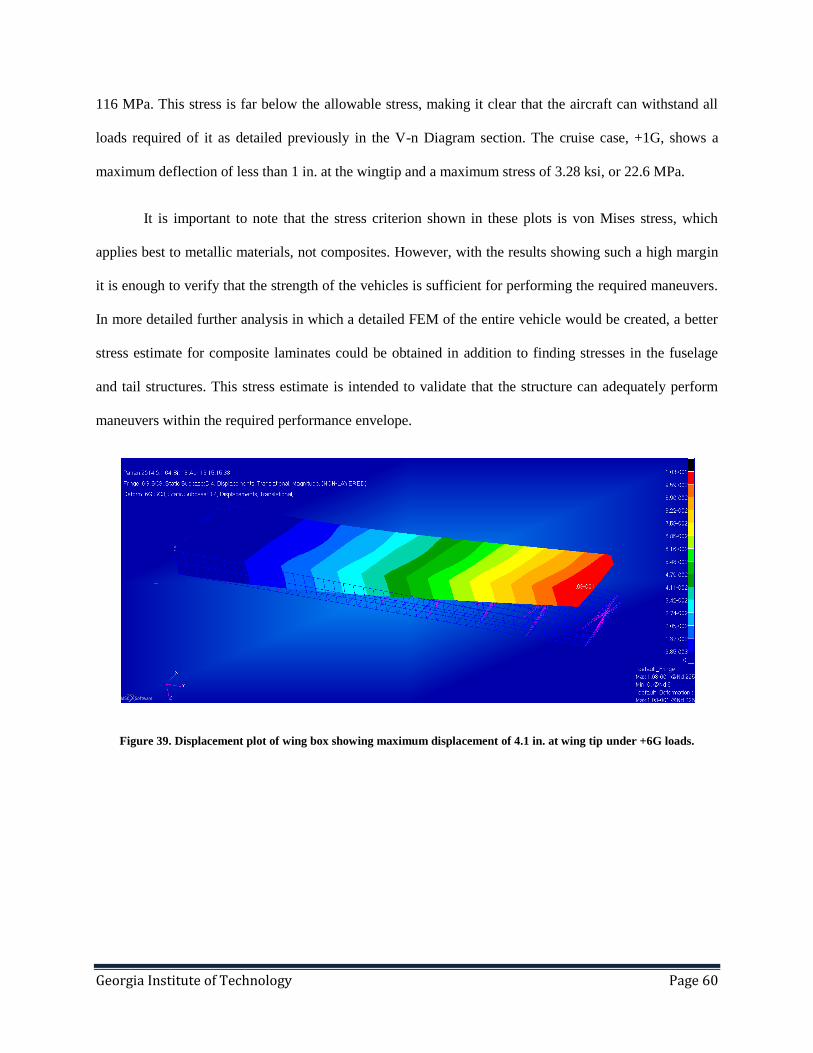
Georgia Institute of Technology Page 60
116 MPa. This stress is far below the allowable stress, making it clear that the aircraft can withstand all
loads required of it as detailed previously in the V-n Diagram section. The cruise case, +1G, shows a
maximum deflection of less than 1 in. at the wingtip and a maximum stress of 3.28 ksi, or 22.6 MPa.
It is important to note that the stress criterion shown in these plots is von Mises stress, which
applies best to metallic materials, not composites. However, with the results showing such a high margin
it is enough to verify that the strength of the vehicles is sufficient for performing the required maneuvers.
In more detailed further analysis in which a detailed FEM of the entire vehicle would be created, a better
stress estimate for composite laminates could be obtained in addition to finding stresses in the fuselage
and tail structures. This stress estimate is intended to validate that the structure can adequately perform
maneuvers within the required performance envelope.
Figure 39. Displacement plot of wing box showing maximum displacement of 4.1 in. at wing tip under +6G loads.

Georgia Institute of Technology Page 61
Figure 40. Stress plot of wing box showing maximum stress of 16.8 ksi near wing root under +6G loads.
Stability and Control
The following stability and control parameters are detailed in this chapter:
Tail Sizing
Control Surface Design
Dynamic Model
Longitudinal Dynamic Modes
Lateral Dynamic Modes
Tail Sizing
A key component in ensuring longitudinal and directional stability of the aircraft lies in the
design of the empennage surfaces. These surfaces must be sized such that the destabilizing effects of the
wing and fuselage about the center of gravity are counterbalanced and the aircraft is stable in typical
flight conditions. First, the sizing and design of the horizontal tail is examined. The main requirement for
the horizontal tail is that the aircraft is longitudinally stable when perturbed. This means that if the aircraft
encounters an upward gust, for example, the aerodynamic forces of the aircraft will act about its center of
gravity to pitch the aircraft down rather than up. To achieve this behavior, the aerodynamic center of the

Georgia Institute of Technology Page 62
aircraft, or the neutral point, must be located further aft than the center of gravity of the aircraft, but not so
far aft that the aircraft is too stable and difficult to maneuver.
After using the volume coefficient method to initially guess the size of the horizontal tail, AVL is
used to refine that guess and produce behavior consistent with an effective aerobatic aircraft. The best
way to define this is to examine the preferences of pilots in a survey. From a survey of aerobatic pilots
performed by Georgia Institute of Technology ASDL, pilots prefer to fly aerobatic missions with the
center of gravity location between 28% and 30% of the mean geometric chord. Given the approximate
horizontal tail size and the general location of each component in the weight and balance, these
percentages correspond to a static margin range of 7-12% for CARL, so this was the target value of static
margin.
After the horizontal tail size is refined using AVL, the static margin of the aircraft can be found at
each significant CG location from the weight and balance. Using AVL to perform the calculations, Table
IX shows the static margin of the aircraft at each CG location. From the table, it is clear that the CG travel
of the single seat version results in a static margin range consistent with that specified above. For the two
seat, the fully loaded version of the aircraft only has a static margin of 9%, and as fuel is used, the margin
moves forward to 5%, which is outside of the ideal range, especially considering the added difficulty of a
low static margin for student pilots when the aircraft flies in a “trainer” capacity. However, the aircraft
has the option to come equipped with a ballast system, which will allow pilots to further tune the CG to fit
their specific mission needs. One final item to note is that if one pilot flies the two seat aircraft from the
front seat, the static margin increases to 27%, which would make the aircraft very stable and difficult to
maneuver.

Georgia Institute of Technology Page 63
Table IX. Static margin of aircraft for significant CG locations.
CG Location Static Margin
Two Seat, Aft-most 5%
Two Seat, Fwd-most 12%
Two Seat, Single Pilot
in Front Seat 27%
Two Seat, Full Load 9%
Single Seat, Aft-most 7%
Single Seat, Fwd-
most/Full Load 12%
Table X shows a summary of the characteristics of the horizontal tail. Some parameters, such as
the area, are chosen to ensure that the neutral point is in the correct location, but other factors such as
sweep, taper, and aspect ratio are chosen to optimize the aerodynamics of the tail and make the design
similar to previous aerobatic aircraft. The airfoil selected is the same as the wing, giving it the same
predictable stall behavior, but because the taper ratio is higher than that of the wing, the stall pattern of
the tail is not as severe as that of the wing.

Georgia Institute of Technology Page 64
Table X. Geometric characteristics of the horizontal tail.
Specification Value
Area (ft2) 25.0
Aspect Ratio 3
Span (ft) 8.7
Sweep (deg) 6.5
Taper 0.8
Root Chord (ft) 3.2
Tip Chord (ft) 2.6
Thickness to Chord (t/c) 0.14
Incidence Angle (deg) 0
Dihedral Angle (deg) 0
Airfoil E474
For the vertical tail, a similar sizing method is used as that for the horizontal tail. For the vertical
tail, the main consideration is directional stability, meaning that under a sideward gust, the aircraft should
be stable and turn into the gust. To achieve this, the vertical tail must be large enough to overcome the
destabilizing effects of the fuselage. After using the approximate volume coefficient from previous
aircraft to obtain an initial guess, AVL is used to determine the yaw moment coefficient with respect to
sideslip angle, or Cn,β, due to the wing and vertical tail. To account for the contribution of the fuselage,

Georgia Institute of Technology Page 65
relations in Nelson’s “Flight Stability and Automatic Control” [14] are used. As a general guideline, Cn,β
should be at least 0.001 per degree. In order to meet this, a vertical tail area of 12 ft2 is selected. Table XI
shows the geometric parameters of the vertical tail, which beyond the area, are chosen with a combination
of being similar to previous aerobatic aircraft and having elegant looks in mind.
Table XI. Vertical tail characteristics for CARL.
Specification Value
Area (ft2) 12.0
Aspect Ratio 1.4
Span (ft) 4.1
Sweep (deg) 30
Taper Ratio 0.5
Root Chord (ft) 3.9
Tip Chord (ft) 2.0
Thickness to Chord (t/c) 0.14
Incidence Angle (deg) 0
Dihedral 90
Airfoil NACA 0014

Georgia Institute of Technology Page 66
Control Surface Design
With the aircraft longitudinally and directionally stable, the next step is to design the control
surfaces of the aircraft, which is very important for aerobatic aircraft. These surfaces must be sized not
only to allow the aircraft to reach trimmed flight in a variety of conditions, but also to ensure that the
aircraft can have a wide envelope to perform the maneuvers required of a competitive aircraft in aerobatic
competitions. To that end, the control surfaces of CARL are oversized by typical criteria. The first control
surface examined is the elevator. The elevator must be designed such that the aircraft can achieve
trimmed flight at its maximum lift coefficient throughout the range of its CG travel. Using AVL,
calculations are performed at each CG location to determine the elevator deflection required to trim. The
allowable elevator deflection is from -25° to 20°, with a negative angle corresponding to an upward
deflection. Table XIII shows the results of the AVL trim analysis with a full-span elevator that covers half
of the horizontal tail chord. As shown in the table, at typical CG locations, the required deflections for
trim leave a wide margin for extra maneuvering, with the exception of a single pilot flying the two seat
aircraft from the front. While this configuration can be trimmed, there is very little extra margin for
maneuvering. The elevator design completes the horizontal tail design. The horizontal tail is shown below
in Figure 41, showing the control surface size and location.

Georgia Institute of Technology Page 67
Table XII. Elevator deflections required to trim CARL at the maximum lift coefficient.
CG Location Elevator Deflection (deg)
Two Seat, Aft-most -2.4
Two Seat, Fwd-most -9.4
Two Seat, One Pilot in
Front Seat -21.9
Two Seat, Full Load -6.4
Single Seat, Aft-most -4.5
Single Seat,
Fwd-most/Full Load
-9.0

Georgia Institute of Technology Page 68
Figure 41. Dimensioned three-view of horizontal tail showing tail and elevator size and location (dimensions in inches).
The rudder is designed with several factors in mind. These include controlling the aircraft during
crosswind landings, correcting for adverse yaw during turns, and allowing the aircraft to recover from a
spin. Because the aircraft is aerobatic, the latter requirement is the most important. In order to optimize
the aircraft for this condition, the horizontal tail is placed as high as possible in the rear section of the
aircraft. Additionally, the rudder is assumed to be 50% of the vertical tail and have a maximum deflection
of 20° in either direction. While a detailed dynamic analysis of this condition is beyond the scope of this
report, using relations in Nelson and calculations from AVL, this airplane configuration and large rudder
should allow the aircraft to meet this requirement. A dimensioned three-view of the vertical tail showing
the rudder size and location is shown below.

Georgia Institute of Technology Page 69
Figure 42. Dimensioned three-view of vertical tail showing tail and rudder size and location (dimensions in inches).
The final control surface examined is the “flaperons” along the wings. Due to the relatively high
roll rate required by the aerobatic aircraft, the decision is made to combine the functions of the flaps and
the ailerons into one control surface. While this adds complexity to the design of the control system, the
performance benefits in roll and during takeoff and landing are high enough that it is deemed an
acceptable tradeoff. The roll requirement from the RFP is that the aircraft should be able to reach a steady
state roll rate of 180 degrees per second at 120 knots CAS. To meet this, the span of the flaperons is
assumed to be from 15% to 93% of the span of each wing, the chord is assumed to be 25% of the wing,
and the maximum deflection in either direction is assumed to be 20°. It is shown in the Dynamic Model
section of this report that this configuration allows the aircraft to exceed the roll rate requirement.
Additionally, when used in the flap capacity, by using calculation methods for plain flaps shown in
Roskam Part II [17], the aircraft CL,max is increased from 1.45 to 2.0 when the flaps are at maximum
deflection, boosting the takeoff and landing performance of the aircraft. A dimensioned three-view of the

Georgia Institute of Technology Page 70
wing showing the flaperons size and location is given below. Table XIII summarizes the control surface
design of the aircraft.
Figure 43. Dimensioned three-view of wing showing flaperon size and location (dimensions in inches).

Georgia Institute of Technology Page 71
Table XIII. Summary of control surface design for CARL.
Elevator Rudder Flaperon
Maximum Deflection (deg) -25/20 -20/20 -20/20
Span Full Full 15% to 93%
Chord 50% 50% 25%
Dynamic Model
With the lifting and control surfaces of the aircraft defined, AVL is used to calculate the stability
derivatives of the aircraft at various flight conditions to create a dynamic model of the aircraft. While
many flight conditions and CG locations of the aircraft are analyzed to determine the dynamics of the
aircraft throughout its flight envelope, only selected results are presented here. The stability derivatives
for the single seat and two seat aircraft, fully loaded and in cruise conditions (110 kts, 7000 ft), are shown
in Table XIV and Table XV respectively. Note that these values are specified in dimensions of per radian.
Table XIV. Aircraft stability derivatives for the single seat version.
CL,α 4.60 CL,β 0 CL,p 0 CL,q 7.02 CL,r 0
CY,α 0 CY,β -0.183 CY,p 0.0689 CY,q 0 CY,r 0.172
Cl,α 0 Cl,β -0.0378 Cl,p -0.434 Cl,q 0 Cl,r 0.0681
Cm,α -0.481 Cm,β 0 Cm,p 0 Cm,q -7.21 Cm,r 0
Cn,α 0 Cn,β 0.0520 Cn,p -0.0213 Cn,q 0 Cn,r -0.108

Georgia Institute of Technology Page 72
Table XV. Aircraft stability derivatives for the two seat version.
CL,α 4.60 CL,β 0 CL,p 0 CL,q 6.72 CL,r 0
CY,α 0 CY,β -0.184 CY,p 0.0788 CY,q 0 CY,r 0.169
Cl,α 0 Cl,β -0.0417 Cl,p -0.433 Cl,q 0 Cl,r 0.0762
Cm,α -0.339 Cm,β 0 Cm,p 0 Cm,q -6.96 Cm,r 0
Cn,α 0 Cn,β 0.0519 Cn,p -0.0239 Cn,q 0 Cn,r -0.107
The stability derivatives Cm,α, Cm,q, Cn,β, and Cn,r, allow the static stability of the aircraft to be
further evaluated according to the criteria in Table XVI. From the table, it is clear that the single seat and
two seat configurations are statically stable in the cruise flight conditions. By examining these derivatives
at different CG locations and throughout the flight envelope of the aircraft, the static stability of CARL is
further verified.
Table XVI. Aircraft static stability for the single and two seat versions during cruise.
Derivative Sign for Stability Ideal Range Single Seat, Cruise
Value (per rad)
Two Seat, Cruise
Value (per rad)
Cm,α Negative -0.3 to -1.5 -0.481 -0.339
Cn,β Positive 0.05 to 0.4 0.0520 0.0519
Cm,q Negative -5 to -40 -7.21 -6.96
Cn,r Negative -0.1 to -1 -0.108 -0.107

Georgia Institute of Technology Page 73
The control surface derivatives of the aircraft are calculated from AVL to complete the dynamics
model. These are shown below for the single and two seat configurations in Table XVII and Table XVIII,
respectively. Note that the flap and the aileron functionality are considered separately in this analysis, and
that the dimensions of each of these derivatives are specified in dimensions of per degree.
Table XVII. Control surface derivatives for the single seat aircraft, with flap and aileron functionality separated.
Aileron Functionality Flap Functionality Elevator Rudder
CL,δa 0 CL,δf 0.0340 CL,δe 0.00864 CL,δr 0
CY,δa -0.000686 CY,δf 0 CY,δe 0 CY,δr 0.00271
Cl,δa 0.00681 Cl,δf 0 Cl,δe 0 Cl,δr 0.000199
Cm,δa 0 Cm,δf -0.00370 Cm,δe -0.0193 Cm,δr 0
Cn,δa 0.000394 Cn,δf 0 Cn,δe 0 Cn,δr -0.00119
Table XVIII. Control surface derivatives for the two seat aircraft, with flap and aileron functionality separated.
Aileron Functionality Flap Functionality Elevator Rudder
CL,δa 0 CL,δf 0.0340 CL,δe 0.00863 CL,δr 0
CY,δa -0.000677 CY,δf 0 CY,δe 0 CY,δr 0.00272
Cl,δa 0.00680 Cl,δf 0 Cl,δe 0 Cl,δr 0.000199
Cm,δa 0 Cm,δf -0.00265 Cm,δe -0.0191 Cm,δr 0
Cn,δa 0.000404 Cn,δf 0 Cn,δe 0 Cn,δr -0.00118

Georgia Institute of Technology Page 74
Using the stability and control derivatives, state space models of the aircraft dynamics linearized
about varying flight conditions are created. These models are split between the longitudinal and lateral
dynamics to extract the dynamic modes from the aircraft. The matrices used for the longitudinal and
lateral dynamics are specified in Nelson [14]. The moments of inertia of the aircraft are approximated
using methods in Roskam Part V [18]. From these methods, the values for the moments of inertia are
shown in Table XIX. Then, using the output angle of attack for each flight condition from AVL, the
moments of inertia of the aircraft are rotated to match its orientation.
Table XIX. Moments of inertia for the single seat and two seat versions.
Inertia Single Seat Two Seat
Ixx (lb-ft2) 394.6 469.8
Iyy (lb-ft2) 451.1 537.0
Izz (lb-ft2) 705.8 840.2

Georgia Institute of Technology Page 75
Longitudinal Dynamic Modes
First, the longitudinal dynamic modes of the aircraft are examined. These modes are typically
split into two behaviors: the short period mode and the phugoid mode. Using tables from Nelson [14], it is
possible to determine the approximate characteristics of these modes required for an aircraft of this size.
These are specified by the aircraft handling qualities. The phugoid mode handling qualities are
characterized by its damping ratio, and are shown in Table XX. The short period mode handling qualities
are characterized by a combination of damping ratio and natural frequency, and are shown in Table XXI.
Note that level one signifies that the flying quality is good, level two signifies that it is acceptable, level
three signifies that improvement is warranted, and below level three means the handling is unacceptable.
Table XX. Flight handling requirements for the phugoid mode.
Flight Handling
Level Requirement
Level 1 ζph > 0.04
Level 2 ζph > 0
Level 3 T2ph > 12 sec
Table XXI. Flight handling requirements for the short period mode.
Flight Handling Level ωnsp Requirement (rad/s) ζsp Requirement
Level 1 2.4 < ωnsp <3.8 ζsp > 0.35
Level 2 1.8 < ωnsp < 6.3 ζsp > 0.25
Level 3 1.8 < ωnsp ζsp > 0.15

Georgia Institute of Technology Page 76
The dynamics model is entered into Matlab and the “damp” function is used to extract the mode
characteristics at each flight condition. Table XXII shows the longitudinal dynamic modes at the cruise
condition. From the table, it is clear that with the exception of flying from the front, the short period mode
meets level two requirements, and the phugoid mode is unstable. The phugoid mode meets level three
requirements because the minimum doubling time is above 12 seconds.
Table XXII. Longitudinal dynamic mode characteristics for both aircraft versions at cruise conditions.
CG Location ζph ωnsp (rad/s) ζsp
Single Seat, Full
Load/Fwd-most -0.068 6.17 0.26
Single Seat, Aft-most -0.068 5.00 0.32
Two Seat, Full Load -0.057 4.89 0.34
Two Seat, Fwd-most -0.057 5.57 0.30
Two Seat, Aft-most -0.057 3.81 0.55
Two Seat, One Pilot in
Front -0.057 8.04 0.21
On the other end of the flight envelope, Table XXIII shows the characteristics of the longitudinal
modes when the aircraft flies at its maximum lift coefficient. From the table, it is clear that the aircraft
still has an unstable phugoid, although now the minimum doubling time is 58 seconds. Additionally, the
short period mode now straddles between level 1 and level 2, depending on the CG location. This furthers
demonstrates how the use of a ballast system with CARL can allow pilots to tune the longitudinal
maneuvering to suit their needs.

Georgia Institute of Technology Page 77
Table XXIII. Longitudinal dynamic mode characteristics for both aircraft versions at maximum CL conditions.
CG Location ζph ωnsp (rad/s) ζsp
Single Seat, Full
Load/Fwd-most -0.012 2.69 0.465
Single Seat, Aft-most -0.012 2.22 0.545
Two Seat, Full Load -0.012 2.23 0.507
Two Seat, Fwd-most -0.012 2.50 0.461
Two Seat, Aft-most -0.012 1.82 0.661
Two Seat, One Pilot
in Front -0.012 3.49 0.364
While the phugoid modes are unstable at each flight condition and only meet level 3
requirements, this is deemed to be acceptable due to the size and mission of the aircraft. Because the
phugoid mode is dominated by slow, long period velocity changes, which will have little effect on the
aerobatics of the aircraft, the fact that this mode is unstable is not very critical. The short period mode, on
the other hand, transitions from level 2 at the cruise condition to level 1 at maximum CL conditions.
Because a significant portion of the maneuvering will be performed at high CL conditions this is a
favorable transition. These behaviors are similar to those of other light sport aircraft.

Georgia Institute of Technology Page 78
Lateral Dynamic Modes
Next, the lateral dynamic modes are examined. These modes are split into three main parts: the
spiral mode, the roll mode, and the Dutch roll mode. The handling qualities for these modes are shown
respectively in Table XXIV, Table XXV, and Table XXVI.
Table XXIV. Flight handling requirements for the spiral mode.
Flight Handling
Level Requirement
Level 1 T2s > 12
Level 2 T2s > 8
Level 3 T2s > 4
Table XXV. Flight handling requirements for the roll mode.
Flight Handling
Level Requirement
Level 1 τroll < 1
Level 2 τroll < 1.4
Level 3 None

Georgia Institute of Technology Page 79
Table XXVI. Flight handling requirements for the Dutch roll mode.
Flight Handling
Level ζDR ωnDR ζDRωnDR
Level 1 > 0.19 > 1 > 0.35
Level 2 > 0.02 > 0.4 > 0.05
Level 3 > 0.02 > 0.04 None
Using the same methodology as for the longitudinal modes, the lateral mode characteristics are
extracted from the lateral dynamics using Matlab. Table XXVII shows the lateral modes for the cruise
condition and Table XXVIII shows the lateral modes for the maximum CL condition. For the cruise
condition, the aircraft meets level 1 handling qualities for every lateral mode. For the maximum CL
condition, on the other hand, the aircraft meets level 1 for the roll and Dutch roll, but is only level 3 for
the spiral mode. In fact, the aircraft does not meet level 3 requirements for the spiral when flown with one
pilot in the front in the two-seat configuration.

Georgia Institute of Technology Page 80
Table XXVII. Lateral mode characteristics for the aircraft cruise condition.
CG Location T2s (sec) τroll (sec) ζDR ωnDR (rad/s) ζDRωnDR
Single Seat, Full
Load/Fwd-most -0.580 0.106 0.411 3.01 1.24
Single Seat, Aft-most -0.584 0.106 0.406 2.96 1.20
Two Seat, Full Load -0.713 0.126 0.374 2.75 1.03
Two Seat, Fwd-most -0.711 0.126 0.377 2.78 1.05
Two Seat, Aft-most -0.717 0.126 0.370 2.71 1.00
Two Seat, Single
Pilot in Front Seat -0.698 0.126 0.391 2.92 1.14

Georgia Institute of Technology Page 81
Table XXVIII. Lateral mode characteristics for the aircraft maximum CL condition.
CG Location T2s (sec) τroll (sec) ζDR ωnDR (rad/s) ζDRωnDR
Single Seat, Full
Load/Fwd-most 4.257 0.285 0.364 1.88 0.69
Single Seat, Aft-most 5.372 0.284 0.360 1.86 0.67
Two Seat, Full Load 5.125 0.340 0.334 1.73 0.58
Two Seat, Fwd-most 4.480 0.341 0.336 1.74 0.59
Two Seat, Aft-most 6.298 0.338 0.331 1.71 0.56
Two Seat, Single
Pilot in Front Seat 2.739 0.348 0.347 1.81 0.63
Like the phugoid mode shown above, the spiral mode is characterized by a slight deviation from
desired flight conditions over time. Because the pilot will have his hand on the stick and be in control of
the aircraft for the vast majority of the aircraft’s mission, the poor spiral mode doubling time is deemed to
be an acceptable tradeoff for this aircraft. It has been seen, however, that the performance of the aircraft
suffers longitudinally and laterally when a pilot flies the two seat aircraft from the front seat, to the point
where the aircraft could be unsafe to fly. Because of this, it is recommended that a single pilot not fly in
the front of the two seat configuration of CARL.
Using Matlab and the dynamic model of the aircraft at 120 knots CAS, it is possible to simulate
the response of the single seat aircraft to its maximum aileron deflection to determine its maximum roll
rate. Figure 44 shows a plot of the roll rate of the aircraft vs. time for a 20-degree aileron input. From the
figure, it is shown that the aircraft achieves a roll rate of 250 degrees per second within a second of

Georgia Institute of Technology Page 82
initiating the roll, and achieves a maximum roll rate of 269 degrees per second, which is much higher than
the 180 degree per second requirement.
Figure 44. Roll rate response to maximum flaperon deflection.
Systems Layout
Here, the systems within the aircraft are described. Systems considered in this section include
avionics and other electrical subsystems, the control system, and a brief discussion of the fuel and smoke
systems.
Avionics
The avionics of the CARL are designed to meet and exceed the standards put forward by ASTM
International in “Standard Specification for Design and Performance of a Light Sport Airplane”
(designation F2245 – 16) sections 8.2 – 8.3.2 [21]. In the following tables, the itemized cost and weight
of the avionics are shown for both aircraft. The displays and instrumentations were predominately priced
and weighted from the Dynon Avionics website [4]. The exception to this being the ignition, toggles, and
antennae that were priced and weighted at aircraft spruce [15]. The one-seat avionics package is very
similar to that of the two seat, but does not require the intercom included in the two-seat package. The
0
50
100
150
200
250
300
0 1 2 3 4
Ro
ll R
ate
(de
g/s)
Time (s)

Georgia Institute of Technology Page 83
tilde under the cost of two autopilot servos is present because that cost is incorporated in the cost of the
autopilot interface.
Table XXIX. Two-seat avionics package cost and weight breakdown.
Component Cost (2016 USD) Weight (lb)
Back Panel
7" display (EFIS-D100 super bright) $ 2,550.00 2.3
Autopilot Interface $ 3,700.00 0.65
VHF Com (25 kHz) $ 1,239.00 0.75
3-1/8" Engine Monitoring System (EMS-D10) $ 1,700.00 1.25
Keyed Ignition $ 137.00 0.1
Toggles (x6) $ 72.00 0.3
Intercom $ 295.00 0.45
Front Panel
7" display (EFIS-D100 super bright) $ 2,550.00 2.3
VHF Com (25 kHz) $ 1,239.00 0.75
3-1/8" Engine Monitoring System (EMS-D10) $ 1,700.00 1.25
Toggles (x6) $ 72.00 0.3
Intercom $ 295.00 0.45
Internal
Transponder $ 1,800.00 0.9
Battery Pack (x2) $ 260.00 1.8
Heated Pitot Probe $ 450.00 0.5
Autopilot Servo (x2) ~ 6
Engine Sensors $ 345.00 2
VHF Com Antenna $ 170.00 0.5
Transponder Antenna $ 140.00 0.25
Additional Cables + Harnesses $ 220.00 3.6
Pilot Monitoring Safety System $ 92.00 0.3
Total $ 19,096.00 26.7

Georgia Institute of Technology Page 84
Table XXX. One-Seat avionics package cost and weight breakdown.
Component Cost (2016 USD) Weight (lb)
Panel
7" display (EFIS-D100 super bright) $ 2,550.00 2.3
Autopilot Interface $ 3,700.00 0.65
VHF Com (25 kHz) $ 1,239.00 0.75
3-1/8" Engine Monitoring System (EMS-D10) $ 1,700.00 1.25
Keyed Ignition $ 137.00 0.1
Toggles (x6) $ 72.00 0.3
Internal
Transponder $ 1,800.00 0.9
Battery Pack $ 130.00 0.9
Heated Pitot Probe $ 450.00 0.5
Autopilot Servo (x2) ~ 6
Engine Sensors $ 345.00 2
VHF Com Antenna $ 170.00 0.5
Transponder Antenna $ 140.00 0.25
Additional Cables + Harnesses $ 40.00 1.4
Pilot Monitoring Safety System $ 72.00 0.3
Total $ 12,545.00 18.1
In an effort to reduce weight and modernize the aircraft, the avionics packages include digital
displays instead of heavier mechanical gauges. With vital flight data being digital, there is a risk of a
power outage in the aircraft being very hazardous. To mitigate this risk, in addition to the large central
APU that the avionics and electrical systems run on, there are backup batteries integrated to keep vital
flight data accessible to the pilot in the event of a power outage.
In Figure 45, a notional layout of the avionics and instrumentation is provided for the back panel
of the two-seat CARL. Similarly, the corresponding front panel is shown in Figure 46.

Georgia Institute of Technology Page 85
Figure 45. Avionics and instrumentation panel: two-seat aircraft, back panel.
Figure 46. Avionics and instrumentation panel: two-seat aircraft, front panel.
Although it is not necessary to have some of the same features on the front panel as the back, it is
a nice touch to have some of the controls, radio, and engine monitoring display in the front seat as well
for training a new pilot. The CARL aircraft family offers a great panel standard, and has ample space for
an owner to upgrade to a larger or second screen and tailor the experience to their own liking.
An intercom is provided to ease communication between the pilots in tandem seating, and an
autopilot interface allows the back pilot to control the autopilot system. The autopilot interface coupled
with the pilot monitoring system offers one of the CARL family’s most notable features. The pilot has
full control over the two-axis autopilot system as with any autopilot interface. However, there is also a
pilot monitoring system that will auto-engage the autopilot system if the pilot goes unconscious during a
high g maneuver. The safety system can to be activated and deactivated at the pilots will, so it does not
auto-engage at undesirable times. The pilot monitoring system consists of several large pressure sensitive

Georgia Institute of Technology Page 86
resistors mounted in the stick handle and a small single board computer integrated with the autopilot
interface and toggles for pilot control. This system adds a layer of safety for the unique increased risk
associated with the mission profile of an aerobatic plane in a way that has never been done before.
Figure 47 shows the panel for the single-seat variant. The only difference between this panel and
the back panel of the two-seat variant is the absence of a pilot-to-pilot intercom.
Figure 47. Avionics and instrumentation panel: single-seat aircraft.
Figure 48. Avionics and instrumentation panel visualization: two-seat back panel. [Displays: Ref. [4] and [12]]

Georgia Institute of Technology Page 87
In Figure 48 above, a more realistic visualization of the control panel from the pilots’ point of
view is provided. Some margin is built into the cost and weight in the additional cables and harnesses
section. All the necessary cables and harnesses for the equipment is listed, however, some additional
cables or cable management systems may be needed when a more detailed design is arrived at.
Electrical Systems
In addition to the electronics in the avionics, only a few additional electrical systems are a part of
the aircraft. Lights on the wing tips and tail are included in the electrical systems of the plane in
accordance to standards for LSA in “Standard Specification for Design and Performance of a Light Sport
Airplane” in turms of location and range of visibility [21]. The speed limiter for the engine also requires
power from the elecrical system. Overall, the avionics and instrumentation such as the heated pitot probe
and anteani make up the majority of the electrical system in the plane. Space in the structural depth of the
aircraft will be used for wiring, with tubing and grommets to protect the wiring.
Control Systems
The CARL aircraft has three major control surfaces: ailerons, elevators, and a rudder. These
control surfaces are controlled by the pilot through a stick and pedals in the cockpit. These control inputs
are transmitted to the surfaces through cables.
By specifying maximum control input travel and corresponding maximum surface deflection, a
gearing ratio for each control system was specified. In Table XXXI, the surface travel, stick travel, and
gearing ratios for each control system are given.
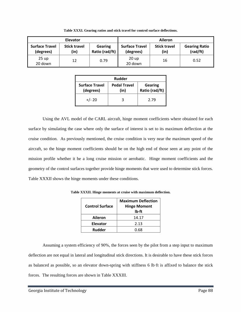
Georgia Institute of Technology Page 88
Table XXXI. Gearing ratios and stick travel for control surface deflections.
Elevator Aileron
Surface Travel (degrees)
Stick travel (in)
Gearing Ratio (rad/ft)
Surface Travel (degrees)
Stick travel (in)
Gearing Ratio (rad/ft)
25 up 20 down
12 0.79 20 up
20 down 16 0.52
Rudder
Surface Travel (degrees)
Pedal Travel (in)
Gearing Ratio (rad/ft)
+/- 20 3 2.79
Using the AVL model of the CARL aircraft, hinge moment coefficients where obtained for each
surface by simulating the case where only the surface of interest is set to its maximum deflection at the
cruise condition. As previously mentioned, the cruise condition is very near the maximum speed of the
aircraft, so the hinge moment coefficients should be on the high end of those seen at any point of the
mission profile whether it be a long cruise mission or aerobatic. Hinge moment coefficients and the
geometry of the control surfaces together provide hinge moments that were used to determine stick forces.
Table XXXII shows the hinge moments under these conditions.
Table XXXII. Hinge moments at cruise with maximum deflection.
Control Surface Maximum Deflection
Hinge Moment lb·ft
Aileron 14.17
Elevator 2.13
Rudder 0.68
Assuming a system efficiency of 90%, the forces seen by the pilot from a step input to maximum
deflection are not equal in lateral and longitudinal stick directions. It is desirable to have these stick forces
as balanced as possible, so an elevator down-spring with stiffness 6 lb·ft is affixed to balance the stick
forces. The resulting forces are shown in Table XXXIII.

Georgia Institute of Technology Page 89
Table XXXIII. Stick and pedal forces seen by pilot.
Control Surface Maximum Stick
Force (lbf)
Aileron 8.25
Elevator 8.53
Rudder 12.10
Figure 49 shows the relatively simple cable control system and how it will be contained within a
small portion of the fuselage. The one-seat variant is a slightly less complicated version of the two-seat
control system layout pictured.
Figure 49. Control system layout.
Fuel System
At its maximum capacity, the fuel tank holds 85 lb of fuel, or 14 US gallons. In Figure 50, the
fuel tank is shown placed in the fuselage. The fuel tank fits within the area designated in the side view of
the CARL aircraft and keeps 3-4 inches of clearance between it and the fuselage wall for structure. It is
sized to hold all the required fuel and still contain a pressurization system within the volume. The
pressurization of the fuel tanks allows the aircraft to fly inverted for long durations without starving the
Georgia Institute of Technology Page 90
engine. Between the fuel tank and pressurization system is a firewall to prevent the fuel and other
components from burning in the event of an engine fire.
Figure 50. Fuel tank in fuselage.
Smoke System
Integrated into the design of the CARL aircraft is an 8-gallon smoke system. This smoke system
offers an easy built in option for adding smoke to the owner’s aerobatic performance. The smoke system
is optional and located bellow the fuel tank right above the exhaust port that it exits the plane through. Its
location and weight range (± 28 lb) means the effects on static margin and balance are minimal as it is
emptied throughout the course of the flight. The System provides over five minutes of smoke to add
pizzazz to any performance.
Cost and Business Plan
The cost of the CARL aircraft varies based on the variant (one-seat or two-seat) and the options
selected to be included in the purchase of the aircraft. In this section, the acquisition cost and operational
cost will be discussed. Optional features and the price reductions associated with their removal are
covered. In addition, the cost model used to price the aircraft, as well as a brief market analysis, is
presented.

Georgia Institute of Technology Page 91
The Cost Model
When it comes to cost models for aircraft, the most complete and in-depth model to date is the
DAPCA IV (Development And Procurement Costs of Aircraft) released by the Rand Corporation in 1987
[6]. This model however, is based solely on military aircraft and greatly over-estimates the cost of
general aviation aircraft and the like. More recently, Charles Eastlake at Embry-Riddle Aeronautical
University altered the DAPCA IV model to better represent general aviation aircraft [3]. The paper in
reference 7 gives a lot of useful information and general rules for applying the model, but does not list
any of the equations or actual method. The equations used in this cost model are from professor Eastlakes
work, but are presented in a publication by a collogue of his at Embry-Riddle. General Aviation Aircraft
Design by Snorri Gudmundsson is the source of the equations and method used to estimate the cost
associated with producing the CARL aircraft [8].
This model gives estimates for major production costs such as material, manufacturing, and
certification, as well as operational costs such as yearly inspections, storage, and engine refurbishing
funds. However, it leaves a few recurring costs such as avionics, engine, and the smoke system to be
calculated separately and added to the total with some quantity discount. The quantity discount assumes
that full cost will not be paid for items that can be bought in large quantities directly from the
manufacture. As pointed out by Gudmundsson, the quantity discount factor used in the DAPCA IV of 0.8
suggests that these items could be purchased for just 10% of their listed price if 1,000 units are bought.
For the purposes of pricing the CARL, a more reasonable quantity discount factor of 0.95 was applied.
By far, the most sizable costs not associated with the development and manufacturing process are
the engine and avionics. Unfortunately, unlike the avionics, the precise cost of the engine in the CARL is
not yet known. The cost model gives an equation for approximating this cost, but it utilizes a linear
model meant to cover a large range of aircraft, many of which are much larger than the CARL. In order
to ensure as accurate an estimate as possible, the cost of 22 engines for aerobatic aircraft were plotted as a
function of horsepower. Figure 51 shows the engine data plotted with a trend line as well as the estimate
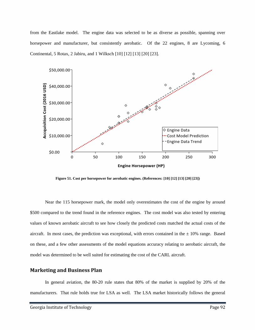
Georgia Institute of Technology Page 92
from the Eastlake model. The engine data was selected to be as diverse as possible, spanning over
horsepower and manufacturer, but consistently aerobatic. Of the 22 engines, 8 are Lycoming, 6
Continental, 5 Rotax, 2 Jabiru, and 1 Wilksch [10] [12] [13] [20] [23].
Figure 51. Cost per horsepower for aerobatic engines. (References: [10] [12] [13] [20] [23])
Near the 115 horsepower mark, the model only overestimates the cost of the engine by around
$500 compared to the trend found in the reference engines. The cost model was also tested by entering
values of known aerobatic aircraft to see how closely the predicted costs matched the actual costs of the
aircraft. In most cases, the prediction was exceptional, with errors contained in the ± 10% range. Based
on these, and a few other assessments of the model equations accuracy relating to aerobatic aircraft, the
model was determined to be well suited for estimating the cost of the CARL aircraft.
Marketing and Business Plan
In general aviation, the 80-20 rule states that 80% of the market is supplied by 20% of the
manufacturers. That rule holds true for LSA as well. The LSA market historically follows the general
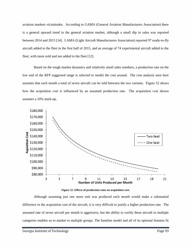
Georgia Institute of Technology Page 93
aviation markets vicissitudes. According to GAMA (General Aviation Manufacturers Association) there
is a general upward trend in the general aviation market, although a small dip in sales was reported
between 2014 and 2015 [14]. LAMA (Light Aircraft Manufacturers Association) reported 97 ready-to-fly
aircraft added to the fleet in the first half of 2015, and an average of 74 experimental aircraft added to the
fleet, with more sold and not added to the fleet [12].
Based on the tough market dynamics and relatively small sales numbers, a production rate on the
low end of the RFP suggested range is selected to model the cost around. The cost analysis seen here
assumes that each month a total of seven aircraft can be sold between the two variants. Figure 52 shows
how the acquisition cost is influenced by an assumed production rate. The acquisition cost shown
assumes a 10% mark-up.
Figure 52. Effects of production rates on acquisition cost.
Although assuming just one more unit was produced each month would make a substantial
difference in the acquisition cost of the aircraft, it is very difficult to justify a higher production rate. The
assumed rate of seven aircraft per month is aggressive, but the ability to certify these aircraft in multiple
categories enables us to market to multiple groups. The baseline model and all of its optional features fit

Georgia Institute of Technology Page 94
under the light-sport requirements for certification, but with a different propeller design the maximum
speed of the aircraft would easily be raised above 120 kts and the certification would have to change to
experimental. Similarly, by selling the aircraft as kits instead of fully assembled the CARL aircraft is able
to appeal to the homebuilt market and certify experimental there as well. Without these broad certification
options, the CARL aircraft market would be much narrower and a production rate of seven aircraft per
month would be very optimistic.
With both aircraft, certain features are optional. Offering optional avionics packages and features
allows for the base level cost of the aircraft to be quite competitive with similar aircraft. Among the
optional features are three levels of avionics packages, removal of the smoke system, and removal of the
ballast system. Exact acquisition costs of each aircraft and options package is discussed in the following
section.
In addition to the options above, a market strategy for the future is the removal of the rpm limiter
on the engine, engine and propeller upgrades, as well as a heavier airframe that can take higher g loads.
These changes would move the aircraft out of the LSA category and into the experimental category, and
make it highly competitive in any aerobatic competition tier. This would open a new market up for the
CARL aircraft without necessitating a major redesign of the aircraft. Another market that may be tapped
in the future is the home-built market. Moving into these markets after the design has been tested in the
LSA market would be a smart way to increase revenue in future years.
Due to the commonality between the two aircraft, the cost model assumes that there is a shared
learning curve in manufacturing as well as a shared quantity discount. At the price point discussed in the
next section, 244 aircraft must be sold to break even. This corresponds to just under 3 years at this
production rate.

Georgia Institute of Technology Page 95
Assuming that the price of the aircraft is fixed, it is worth examining the results of sales numbers
that do not match the assumed production rate. Figure 53 shows annual revenue for a range of unit sales
per month at the current price point.
Figure 53. Sales effect on annual revenue at cost point.
Below seven units per month, the units required to break even increases rapidly, and below 5.5
units a month, the aircraft will never break even or produce a profit for the company. If however, the
aircraft becomes a hit, the revenue from the planes double if just 2.5 more units are sold each month than
projected. Also evident in the graph is that there is almost no advantage to selling more of one variant.
Acquisition Cost
Using the cost model discussed, an acquisition cost for the aircraft was estimated for both the one
and two-seat variants. The cost data presented in Table XXXIV represents the two-seat variant with all
the options (most expensive packages). As stated there, the price at market is just under $134,000. The
acquisition cost covers the cost of producing the aircraft as well as product liability and a mark-up of
10%.
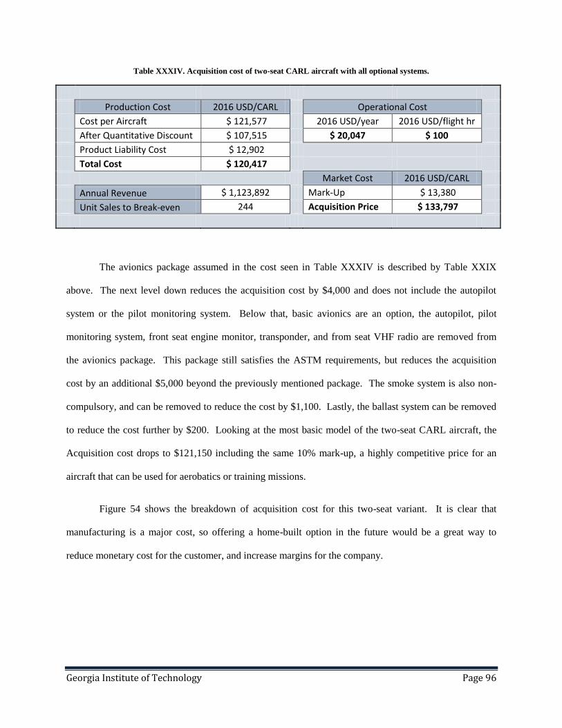
Georgia Institute of Technology Page 96
Table XXXIV. Acquisition cost of two-seat CARL aircraft with all optional systems.
Production Cost 2016 USD/CARL Operational Cost
Cost per Aircraft $ 121,577 2016 USD/year 2016 USD/flight hr
After Quantitative Discount $ 107,515 $ 20,047 $ 100
Product Liability Cost $ 12,902
Total Cost $ 120,417
Market Cost 2016 USD/CARL
Annual Revenue $ 1,123,892 Mark-Up $ 13,380
Unit Sales to Break-even 244 Acquisition Price $ 133,797
The avionics package assumed in the cost seen in Table XXXIV is described by Table XXIX
above. The next level down reduces the acquisition cost by $4,000 and does not include the autopilot
system or the pilot monitoring system. Below that, basic avionics are an option, the autopilot, pilot
monitoring system, front seat engine monitor, transponder, and from seat VHF radio are removed from
the avionics package. This package still satisfies the ASTM requirements, but reduces the acquisition
cost by an additional $5,000 beyond the previously mentioned package. The smoke system is also non-
compulsory, and can be removed to reduce the cost by $1,100. Lastly, the ballast system can be removed
to reduce the cost further by $200. Looking at the most basic model of the two-seat CARL aircraft, the
Acquisition cost drops to $121,150 including the same 10% mark-up, a highly competitive price for an
aircraft that can be used for aerobatics or training missions.
Figure 54 shows the breakdown of acquisition cost for this two-seat variant. It is clear that
manufacturing is a major cost, so offering a home-built option in the future would be a great way to
reduce monetary cost for the customer, and increase margins for the company.
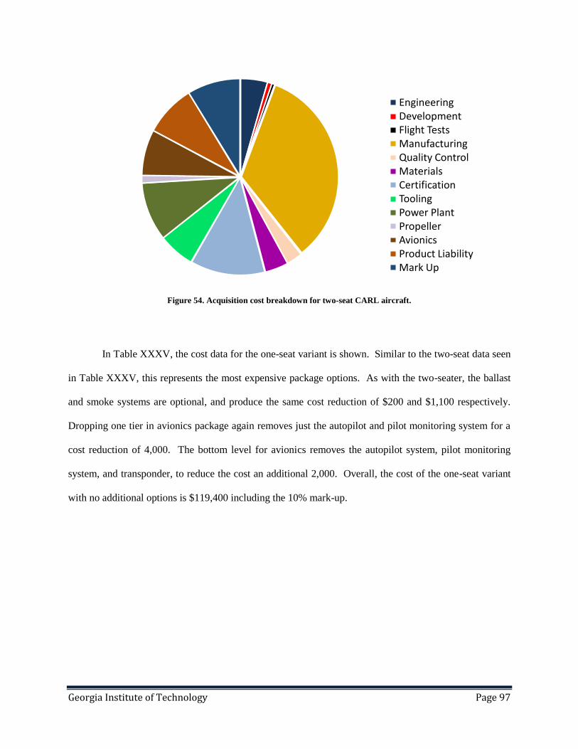
Georgia Institute of Technology Page 97
Figure 54. Acquisition cost breakdown for two-seat CARL aircraft.
In Table XXXV, the cost data for the one-seat variant is shown. Similar to the two-seat data seen
in Table XXXV, this represents the most expensive package options. As with the two-seater, the ballast
and smoke systems are optional, and produce the same cost reduction of $200 and $1,100 respectively.
Dropping one tier in avionics package again removes just the autopilot and pilot monitoring system for a
cost reduction of 4,000. The bottom level for avionics removes the autopilot system, pilot monitoring
system, and transponder, to reduce the cost an additional 2,000. Overall, the cost of the one-seat variant
with no additional options is $119,400 including the 10% mark-up.
Engineering Development Flight Tests Manufacturing Quality Control Materials Certification Tooling Power Plant Propeller Avionics Product Liability Mark Up

Georgia Institute of Technology Page 98
Table XXXV. Acquisition cost of the one-seat CARL aircraft with all optional systems.
Production Cost 2016 USD/CARL Operational Cost
Cost per Aircraft $ 115,116 2016 USD/year 2016 USD/flight hr
After Quantitative Discount $ 103,383 $ 19,663 $ 98
Product Liability Cost $ 12,406
Total Cost $ 115,789
Market Cost 2016 USD/CARL
Annual Revenue $ 1,080,697 Mark-Up $ 12,865
Unit Sales to Break-even 244 Acquisition Price $ 128,654
Figure 55 below shows the breakdown of cost for the one-seat variant. It is similar to that seen
for the two-seat variant, with the main difference being the smaller percentage associated with avionics.
Figure 55. Acquisition cost breakdown of the one-seat CARL aircraft.
Engineering Development Flight Tests Manufacturing Quality Control Materials Certification Tooling Power Plant Propeller Avionics Product Liability Mark Up

Georgia Institute of Technology Page 99
Life Cycle Cost
In Table XXXIV and Table XXXV above, operational costs for both aircraft are shown in the top
right. Included in the operational cost is a loan payment that assumes a 20% down payment and a 15-year
payment plan on the loan for the aircraft. This means that much of the acquisition cost is wrapped up in
the cost of ownership through the loan payment. Also in the operational cost is the cost of storing the
aircraft, maintenance, inspections, fuel, insurance, and an engine overhaul fund spread over the course of
ten years. The estimate of cost per flight hour assumes around 200 flight hours a year. Figure 56 shows
how these components come together to make up around $20,000 a year in operational costs. Only one
figure breaking down the components is provided because the difference in operational cost proportions is
negligible between the two variants.
Figure 56. Operational cost breakdown for the CARL aircraft.

Georgia Institute of Technology Page 100
References
[1] Advanced Composite Materials. Wellesley Hills, MA: Business Technology Research, 1988. Web.
[2] Anderson, D. Aircraft Performance and Design. McGraw-Hill Education. 1998. Print.
[3] C. N. Eastlake and H. W. Blackwell, "Cost Estimating Software for General Aviation Aircraft Design," in
Proceedings of the ASEE National Conference, St. Louis, MO, 2000.
[4] Composites World. N.p., n.d. Web. 26 Apr. 2016. < http://www.compositesworld.com/articles/fabrication-
methods/>.
[5] Continental Motors, Inc: Factory New and Rebuilt Aircraft Engines. N.p., n.d. Web. 26 Apr. 2016.
<http://www.continentalmotors.aero/>.
[6] Dynon Avionics. N.p., n.d. Web. 26 Apr. 2016. <http://dynonavionics.com/>.
[7] "GAMA - General Aviation Manufacturers Association." GAMA. N.p., n.d. Web. 26 Apr. 2016.
[8] Gudmundsson, S. General Aviation Aircraft Design: Applied Methods and Procedures. Waltham, MA:
Elsevier, 2014. Print.
[9] Hess, Ronald W., and H. P. Romanoff. Aircraft Airframe Cost Estimating Relationships. Santa Monica, CA:
Rand, 1987. Print.
[10] Hoerner, Sighard F. Fluid-dynamic Drag: Practical Information on Aerodynamic Drag and Hydrodynamic
Resistance. Alburqueque, NM: Db Hoerner Fluid Dynamics, 1965. Print.
[11] Jabiru North America LLC. N.p., n.d. Web. 26 Apr. 2016. <http://jabiruna.com/engines>.
[12] "Light Aircraft Manufacturers Association." LAMA Light Aircraft and Sport Aircraft. N.p., n.d. Web. 26
Apr. 2016.
[13] Lycoming. N.p., n.d. Web. <http://www.lycoming.com>.
[14] Nelson, Robert C. Flight Stability and Automatic Control. New York: McGraw-Hill, 1989. Print.
[15] "Pilot Supplies and Aircraft Parts from Aircraft Spruce." N.p., n.d. Web. 26 Apr. 2016.
<http://www.aircraftspruce.com/>.
[16] R. W. Hess and H. P. Romanoff, "Aircraft Airframe Cost Estimating Relationships," RAND Corp., no.
2283/1-AF, 1987.
[17] Roskam, J. (2004). Airplane Design, Part II. Ottawa, Kan.: Roskam Aviation and Engineering.
[18] Roskam, J. (2004). Airplane Design, Part V. Ottawa, Kan.: Roskam Aviation and Engineering.
[19] Roskam, J. (2004). Airplane Design, Part VI. Ottawa, Kan.: Roskam Aviation and Engineering.
[20] Rotax. N.p., n.d. Web. <http://www.flyrotax.com/>.
[21] Standard Specification for Design and Performance of a Light Sport Airplane. West Conshohocken, PA:
ASTM International, 2016. Print.
[22] Toerenbeek, E. Synthesis of Subsonic Airplane Design. N.p.: Delft UP, 1979. Web. 26 Apr. 2016.


