SENSOR-LESS VECTOR CONTROL USING ADAPTIVE OBSERVER SCHEME FOR CONTROLLING THE PERFORMANCE OF THE INDUCTION MOTOR MAZHAR HUSSAIN ABBASI RESEARCH REPORT SUBMITTED IN PARTIAL FULFILLMENT OF THE REQUIREMENT FOR THE DEGREE OF MASTER OF ENGINEERING FACULTY OF ENGINEERING UNIVERSITY OF MALAYA KUALA LUMPUR 2013 University of Malaya
Transcript
SENSOR-LESS VECTOR CONTROL USING ADAPTIVE OBSERVER
SCHEME FOR CONTROLLING THE PERFORMANCE OF THE INDUCTION
MOTOR
MAZHAR HUSSAIN ABBASI
RESEARCH REPORT SUBMITTED IN PARTIAL
FULFILLMENT OF THE REQUIREMENT FOR THE
DEGREE OF MASTER OF ENGINEERING
FACULTY OF ENGINEERING
UNIVERSITY OF MALAYA
KUALA LUMPUR
2013
Univers
ity of
Mala
ya
ii
ORIGINAL LITERARY WORK DECLARATION
Name of the candidate: Mazhar Hussain Abbasi
Registration/Matric No: KGZ110007
Name of the Degree: Master of Engineering (Mechatronics)
Title of Project Paper/ Research Report/ Dissertation / Thesis (“this work”):
Sensorless vector control using adaptive observer scheme for controlling the
performance of induction motor
Field of Study: Electrical machines and drives
I do solemnly and sincerely declare that:
(1) I am the sole author /writer of this work;
(2) This work is original;
(3) Any use of any work in which copyright exists was done by way of fair dealings and
any expert or extract from, or reference or reproduction of any copyright work has been
disclosed expressly and sufficiently and the title of the Work and its authorship has been
acknowledged in this Work;
(4) I do not have any actual knowledge nor ought I reasonably to know that the making
of this work constitutes an infringement of any copyright work;
(5) I, hereby assign all and every rights in the copyrights to this work to the University
of Malaya (UM), who henceforth shall be owner of the copyright in this Work and that
any reproduction or use in any form or by any means whatsoever is prohibited without
the written consent of UM having been first had and obtained actual knowledge;
(6) I am fully aware that in the course of making this Work I have infringed any
copyright whether internationally or otherwise, I may be subject to legal action or any
other action as may be determined by UM.
Candidate’s Signature Date:
Subscribed and solemnly declared before,Witness Signature Date:Name:Designation:
Univers
ity of
Mala
ya
iii
ACKNOWLEDGEMENT
First of all, I would like to express my gratitude to the Almighty Allah, who has created
and gave me strength to finish the dissertation successfully. I remember the esteem,
affection and inspiration of my entire family to complete the degree successfully. I
would like to bestow my gratitude and profound respect to my supervisor Prof. Dr.
Velappa Gounder Ganapathy for his hearty support, encouragement and incessant
exploration throughout my study period.
I am specially acknowledging Mrs. Armarosa for her kind encouragement and
motivation.
I gratefully acknowledging the privileges and opportunities offered by the University of
Malaya. I also express my gratitude to the staff of this varsity that helped directly or
indirectly to produce this piece of work.
Univers
ity of
Mala
ya
iv
ABSTRACT
Sensorless vector control technique using adaptive observer scheme is being used to
control the performance of induction motor which is demonstrated by the help of
matlab/simulink software; a suitable tool for vector control of AC motor. Simulation is
done by using the observer which uses optimal feedback gain as an example of process
from algorithm design to verification of logic. Control design scheme in vector control,
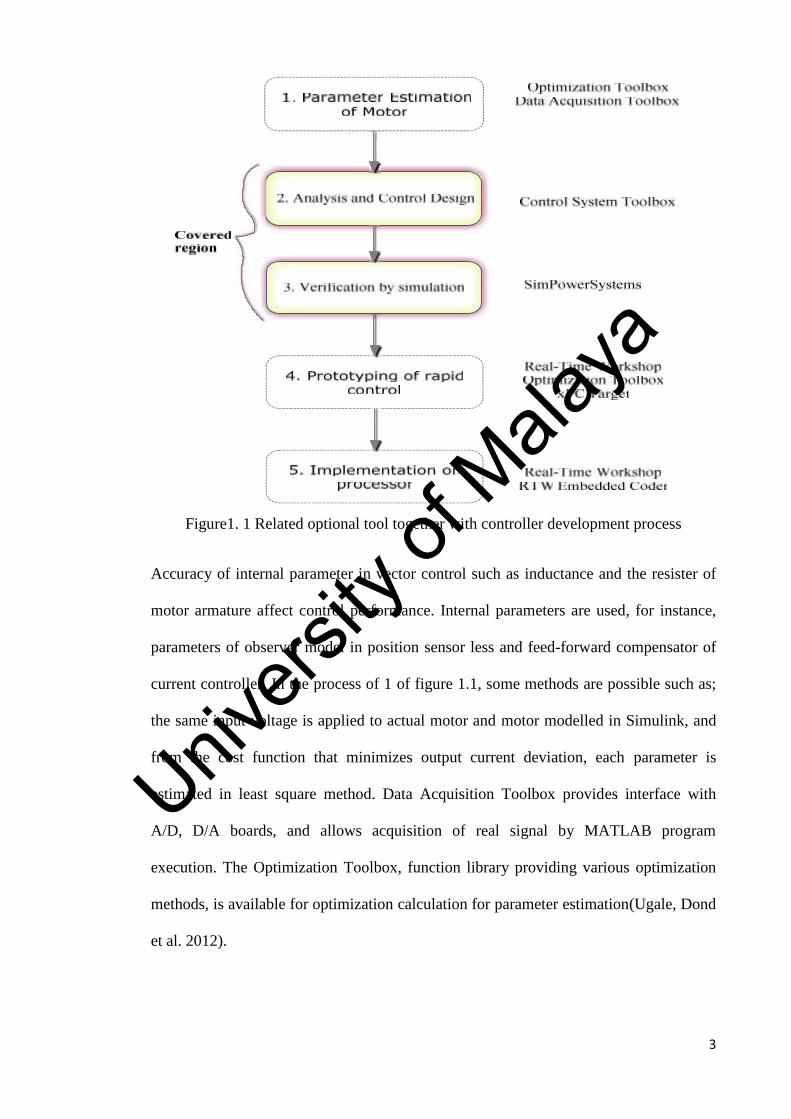
accuracy of internal parameter such as resister of motor armature and inductance affects
control performance. Internal parameters are used, for example, feed-forward
compensator of current controller and parameters of observer model in sensor less
position.
The same technique also can be applied to other types of motor like PMSM. This
adaptive observer is used with the field oriented control of the induction motor. It is
based on using induction motor model with the estimation of the load torque besides the
estimation of the stator resistance and the robustness of this adaptive observer is with
respect to the variation in the resistance of stator. The performance of the suggested
adaptive observer scheme is present on via numerical simulation and the obtained
results from that adaptive observer show the effectiveness of suggested scheme.
Univers
ity of
Mala
ya
v
ABSTRAK
Teknik kawalan vektor tanpa sensor menggunakan skim pemerhati penyesuaian yang
digunakan untuk mengawal prestasi motor aruhan yang ditunjukkan oleh bantuan
perisian MATLAB / SIMULINK; alat yang sesuai untuk kawalan vektor AC motor.
Simulasi dilakukan dengan menggunakan pemerhati yang menggunakan perolehan
maklum balas yang optimum sebagai contoh proses daripada reka bentuk algoritma
untuk pengesahan logik. Skim reka bentuk kawalan dalam kawalan vektor, ketepatan
parameter dalaman seperti rintangan daripada angker motor dan kearuhan
mempengaruhi prestasi kawalan. Parameter dalaman digunakan, sebagai contoh,
pengawal arus pengimbang pemacu-hadapan dan parameter model pemerhati dalam
kedudukan tanpa sensor.
Teknik yang sama juga boleh digunakan untuk lain-lain jenis motor seperti PMSM.
Pemerhati penyesuaian ini digunakan dengan kawalan berorientasikan medan motor
aruhan tersebut. Ini berdasarkan menggunakan model motor aruhan dengan anggaran
tork beban selain anggaran rintangan pemegun dan kekukuhan pemerhati penyesuaian
ini adalah berkenaan dengan perubahan dalam rintangan pemegun. Prestasi cadangan
skim pemerhati penyesuaian ini dibentangkan melalui simulasi berangka dan keputusan
yang diperolehi daripada pemerhati penyesuaian itu menunjukkan keberkesanan skim
yang disyorkan.
Univers
ity of
Mala
ya
vi
TABLE OF CONTENTS
ORIGINAL LITERARY WORK DECLARATION .........................................................ii
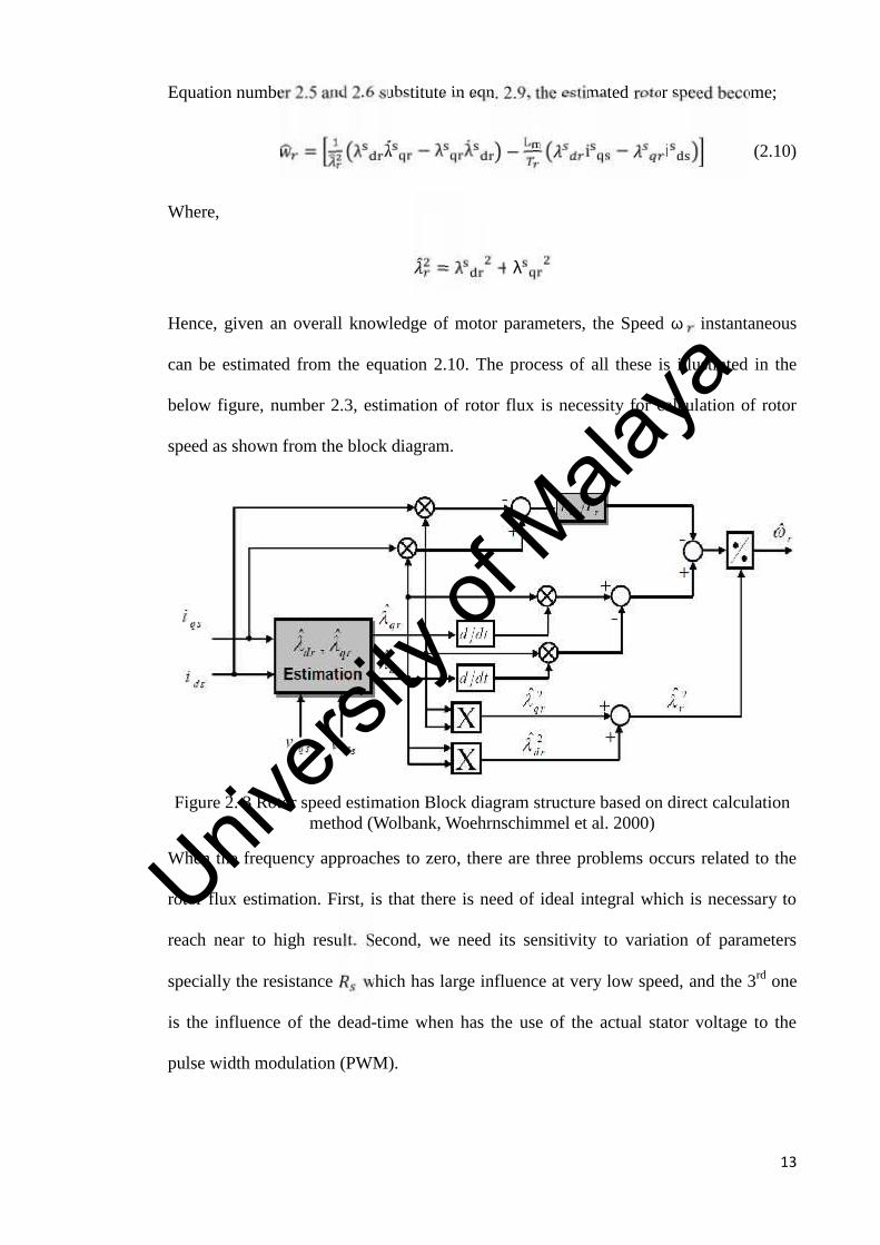
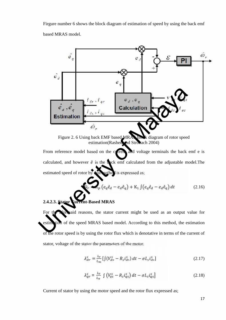
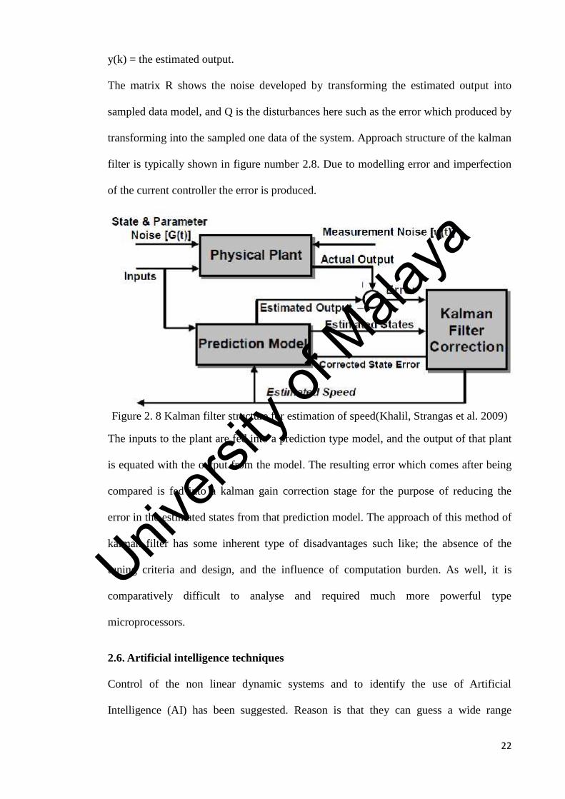
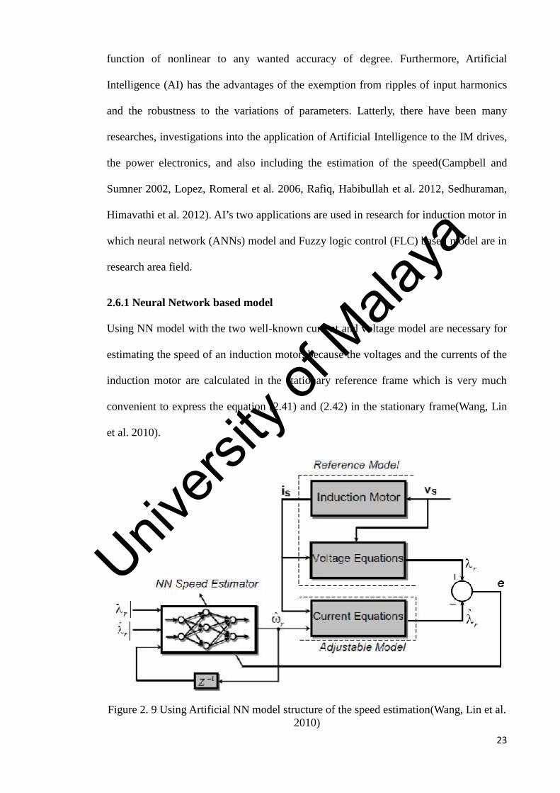
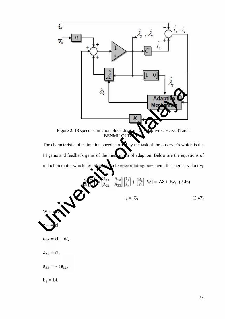
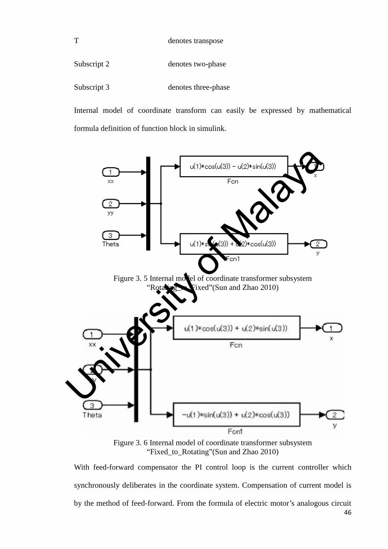
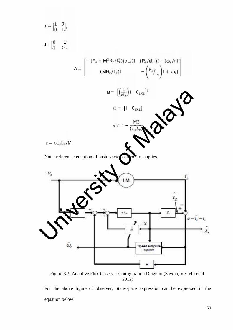
For the above figure of observer, State-space expression can be expressed in the
equation below:
Univers
ity of
Mala
ya
51
= Ax + Bv − H , = (3.5)
Where, H denotes the gain of observer
^ is the estimation value
e is the current error e= i^s – is
A = − (R + M R /L )(σL )I (R /ԑL )I − (ω /ԑ)J(MR /L )I − R L I + ω JThen, parameter adjusting the law of calculation the electric angular velocity (ωr), are
supplied by the below equation using size of outer product of current error vector (e)
and the value of estimation flux:ω = ( r)T
e + ∫( r)T (3.6)
Gain of the observer H is planned in such way to ensure the adaptability of control
system consisting of adaptive observer and the induction motor that is →∞ = .
The term value other than the velocity estimation value, we assume as true value,
equation concerning current error can be showed by subtracting the formulae a3.4 from
a3.5, and define the matrix Bω by separating the term of ω from matrix system.
Therefore, e = C(sI − A + HC)-1 −∆= G( ) −∆ω Jλ (3.7)
Where,∆ = ω − ,I : 4 X 4 ,= ԑ − T
And so, we consider feedback system comprising LTI (linear time invariant) block G(s)
and block of nonlinear time variation similar to the following figure. Applying Popov’s
Univers
ity of
Mala
ya
52
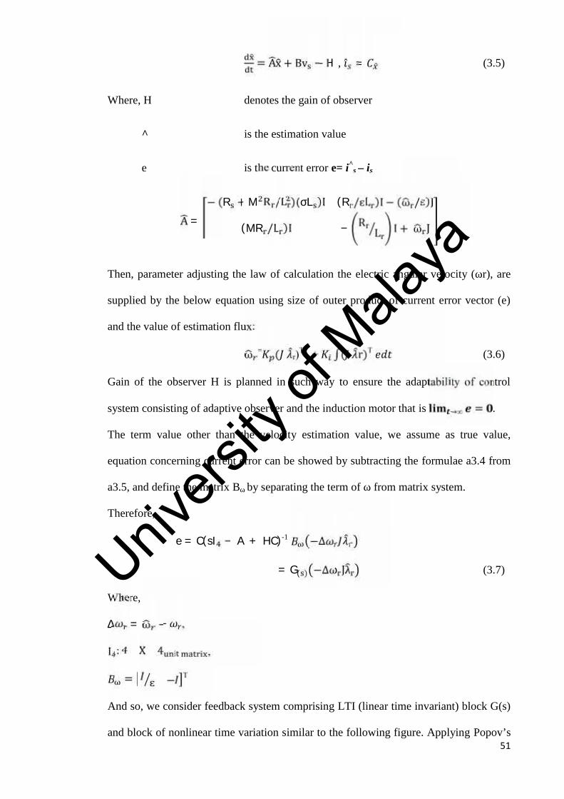
hyper stability, the below are necessary to be satisfied to ensure the stability →∞ =.
1. The Transfer function G(s) of feed forward LTI (Linear − Time − Invariant) isstrictly positive real (SPR).
2. Input v1 and the output w1 of non-linear time variation block satisfy the Popov’s
equation for all the time t1 greater than t0 (t1>t0).∫ > - (3.8)
Where,
: is constant independent of time.
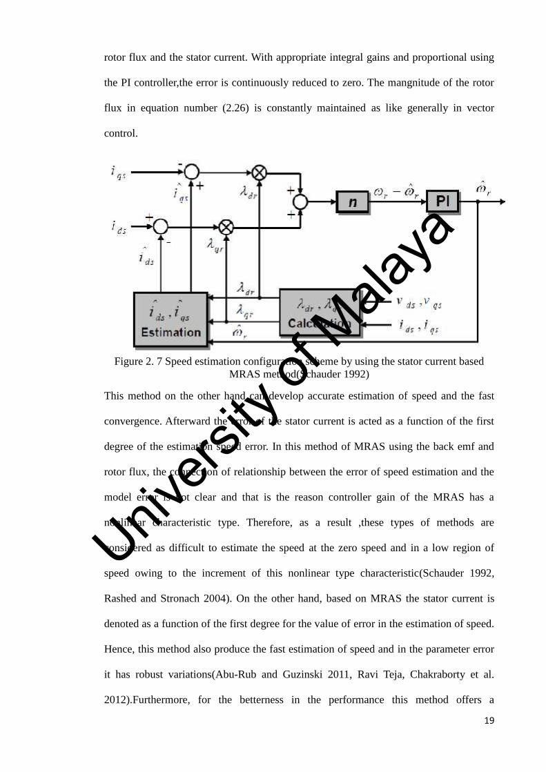
Figure 3. 10 Current error block feedback system (Tarek BENMILOUD 2011)
The above figure is proved to be satisfied by using equation 3.6. Riccati equation is
applied for obtaining the optimal feedback gain to make G(s) SPR as a condition which
we mention above. H = PC R (3.9)
Univers
ity of
Mala
ya
53
Riccati equation: PA + AP − PC R CP + B QB = 0 (3.10)
Where,
P solution of Riccati equation
Q,R weight matrices
The weight matrices Q=1 and R=yI, respectively, however, y is a small positive
number.
3.4 Modeling of Adaptive observer
Program (M-file) of matlab language is used to set the all parameters of motor and each
matrix of state-space expression, and the formula 3.10 is solved with the help of using
the Control System Tool box , and we obtain the optimal feedback gain as well.
Where,
[H, P, E] = lqe(A, Bw, C, Q, R)
The function of Iqe is provided in Control System ToolBox for designing the Kalman
filter estimator and it returns the feedback gain, H, solution of Riccati equation, P, and
pole of estimator E= eig (A-H*C). M-file can be loaded in to the memory (workshop)
once executed in Matlab and define as each block parameter of Simulink model in it.
Adaptive observer subsystem in figure b is defined in figure (3.11) below.
Univers
ity of
Mala
ya
54
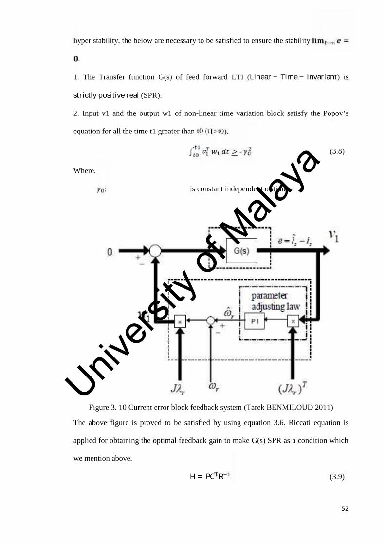
Figure 3. 11 Model of Adaptive Observer
Separate and add none stable term which is ωr that is included in system Matrix A, is
the key to the modelling. Model can be easily done by using the Integrator block in case
motor system is expressed in state-space.
Figure 3. 12 Block diagram inside the Matrix A
54
Figure 3. 11 Model of Adaptive Observer
Separate and add none stable term which is ωr that is included in system Matrix A, is
the key to the modelling. Model can be easily done by using the Integrator block in case
motor system is expressed in state-space.
Figure 3. 12 Block diagram inside the Matrix A
Univers
ity of
Mala
ya
55
Adaptive observer operates stably if the absolute value of the phase difference between
input and out is within 90 degrees. Subsequently it is verified the stableness of the
transfer function G(s) of linear stationary term. Linearization point is indicated as mark
of arrow below in the figure 3.11 is provided by simulink control design is located in
the relevant input and output points.
Hence, stability of transfer functions G(s) is verified. Adaptive observer operates stably
if the absolute value of phase difference between input and output is within 90 degrees.
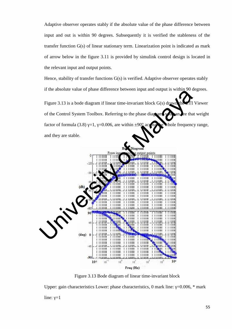
Figure 3.13 is a bode diagram if linear time-invariant block G(s) drawn the LTI Viewer
of the Control System Toolbox. Referring to the phase diagram, you can see that weight
factor of formula (3.8) γ=1, γ=0.006, are within ±90° across the whole frequency range,
and they are stable.
Figure 3.13 Bode diagram of linear time-invariant block
Upper: gain characteristics Lower: phase characteristics, 0 mark line: γ=0.006, * mark
line: γ=1
Univers
ity of
Mala
ya
56
CHAPTER FOUR: RESULTS AND DISCUSSION
Simulations, using MATLAB Software Package, have been carried out to show the
effectiveness of the proposed observer. Model which we discussed in methodology
chapter includes the PI gain that requires tunning for the velocity control, current
controller and velocity estimator.
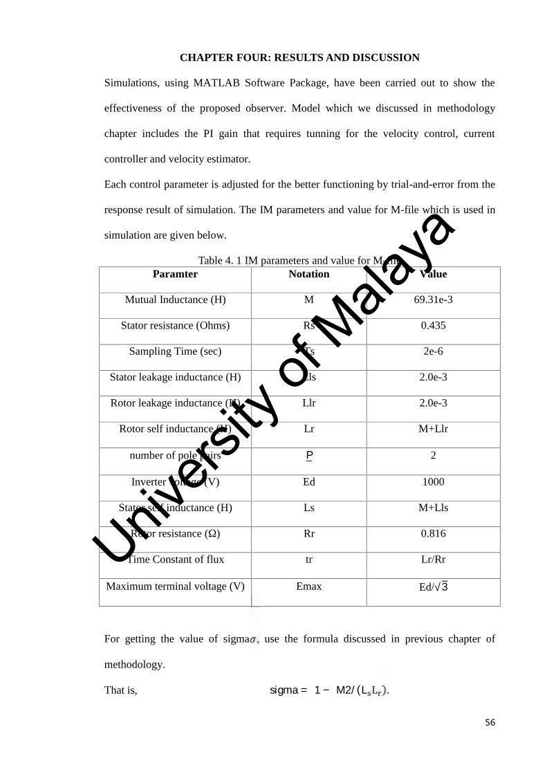
Each control parameter is adjusted for the better functioning by trial-and-error from the
response result of simulation. The IM parameters and value for M-file which is used in
simulation are given below.
Table 4. 1 IM parameters and value for M-fileParamter Notation Value
Mutual Inductance (H) M 69.31e-3
Stator resistance (Ohms) Rs 0.435
Sampling Time (sec) Ts 2e-6
Stator leakage inductance (H) Lls 2.0e-3
Rotor leakage inductance (H) Llr 2.0e-3
Rotor self inductance (H) Lr M+Llr
number of pole pairs P 2
Inverter voltage (V) Ed 1000
Stator self inductance (H) Ls M+Lls
Rotor resistance (Ω) Rr 0.816
Time Constant of flux tr Lr/Rr
Maximum terminal voltage (V) Emax Ed/√3For getting the value of sigma , use the formula discussed in previous chapter of
methodology.
That is, sigma = 1 − M2/(L L ).
Univers
ity of
Mala
ya
57
Value for the State Space Matrix: I = [1 0 : 0 1]J = [0 −1 : 1 0]Compute the variable for state space matrix value with the help of below formulas in M-
file.
A11 = − R + M ∗ RL(sigma ∗ L ) ∗ IA12 = M(sigma ∗ t ∗ L ∗ L ) ∗ I
A21 = Mt ∗ IA22 = − 1t ∗ I
Assigning the variables for memory to workspace variables of space vector:A = [A11 A12 : A21 A22]B = 1(sigma ∗ L ) ∗ I; zeros (2)
C = [I zeros(2)]Bw = [( ∗ ∗ )∗ ; −I]Value of weight matrix: ep = 0.006;R = ep ∗ I;Q = I;For obtaining the optima feed back gain, we can use the formula in M-file, discussed
previously in methodology.
[H, P, E] = lqe(A, Bw, C, Q, R)
Univers
ity of
Mala
ya
58
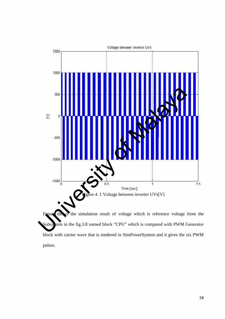
Figure 4. 1 Voltage between inverter UVs[V]
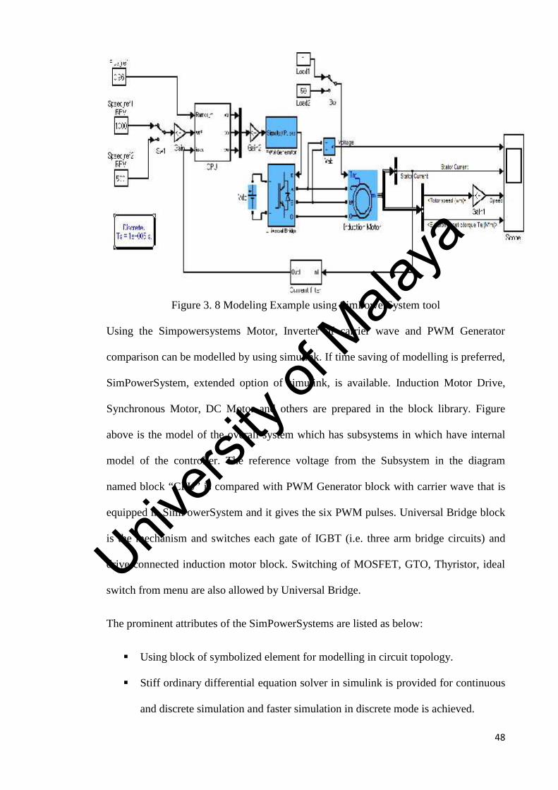
Figure shows the simulation result of voltage which is reference voltage from the
Subsystem in the fig.3.8 named block “CPU” which is compared with PWM Generator
block with carrier wave that is rendered in SimPowerSystem and it gives the six PWM
pulses.
Univers
ity of
Mala
ya
59
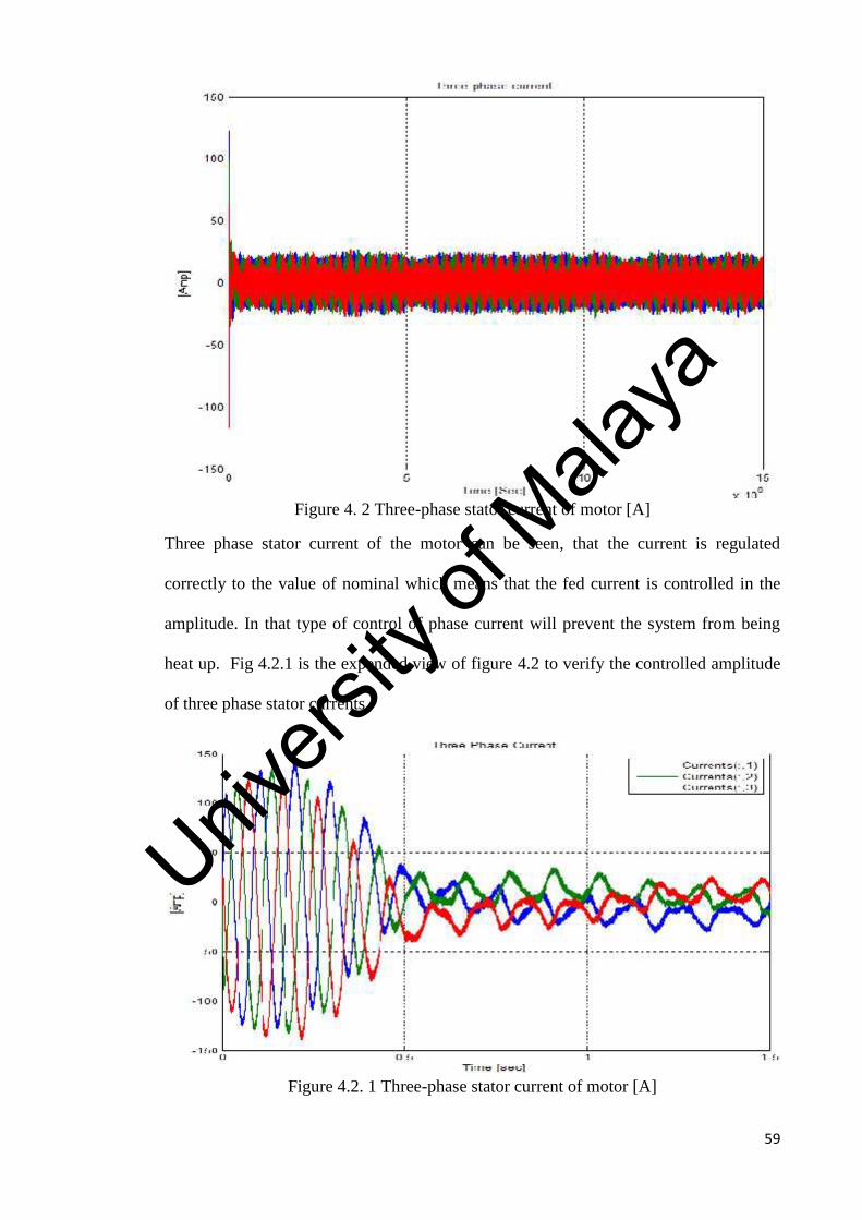
Figure 4. 2 Three-phase stator current of motor [A]
Three phase stator current of the motor can be seen, that the current is regulated
correctly to the value of nominal which means that the fed current is controlled in the
amplitude. In that type of control of phase current will prevent the system from being
heat up. Fig 4.2.1 is the expended view of figure 4.2 to verify the controlled amplitude
of three phase stator currents.
Figure 4.2. 1 Three-phase stator current of motor [A]
Univers
ity of
Mala
ya
60
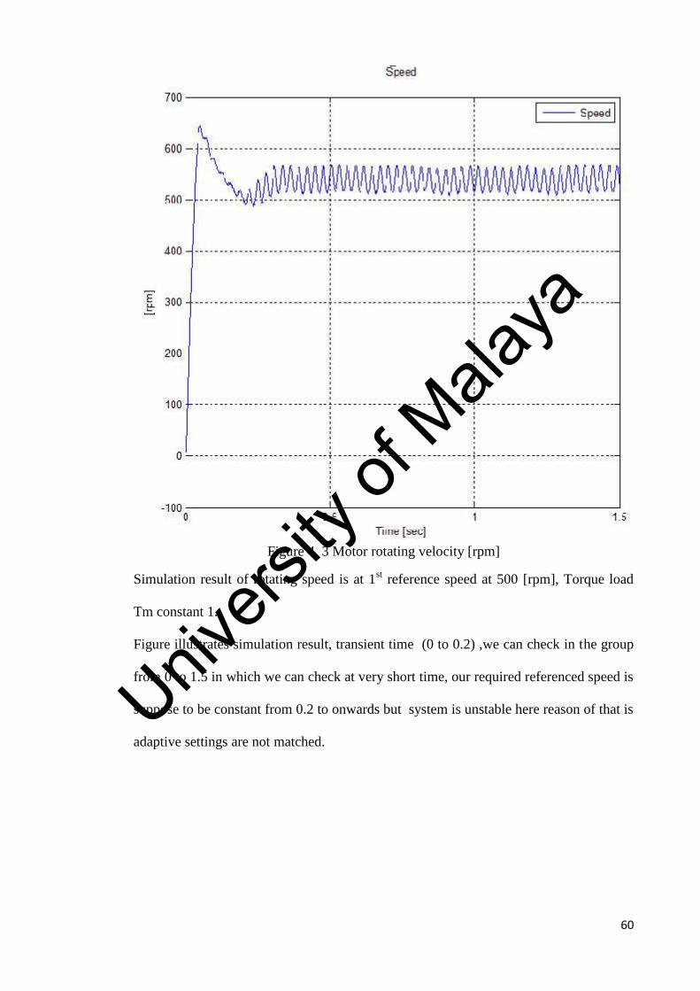
Figure 4. 3 Motor rotating velocity [rpm]
Simulation result of rotating speed is at 1st reference speed at 500 [rpm], Torque load
Tm constant 1.
Figure illustrates simulation result, transient time (0 to 0.2) ,we can check in the group
from 0 to 1.5 in which we can check at very short time, our required referenced speed is
suppose to be constant from 0.2 to onwards but system is unstable here reason of that is
adaptive settings are not matched.Univ
ersity
of M
alaya
61
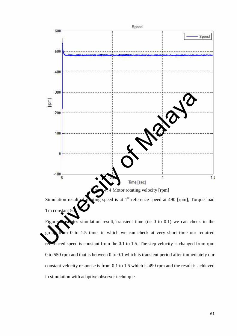
Figure 4. 4 Motor rotating velocity [rpm]
Simulation result of rotating speed is at 1st reference speed at 490 [rpm], Torque load
Tm constant 50.
Figure illustrates simulation result, transient time (i.e 0 to 0.1) we can check in the
group from 0 to 1.5 time, in which we can check at very short time our required
referenced speed is constant from the 0.1 to 1.5. The step velocity is changed from rpm
0 to 550 rpm and that is between 0 to 0.1 which is transient period after immediately our
constant velocity response is from 0.1 to 1.5 which is 490 rpm and the result is achieved
in simulation with adaptive observer technique.
Univers
ity of
Mala
ya
62
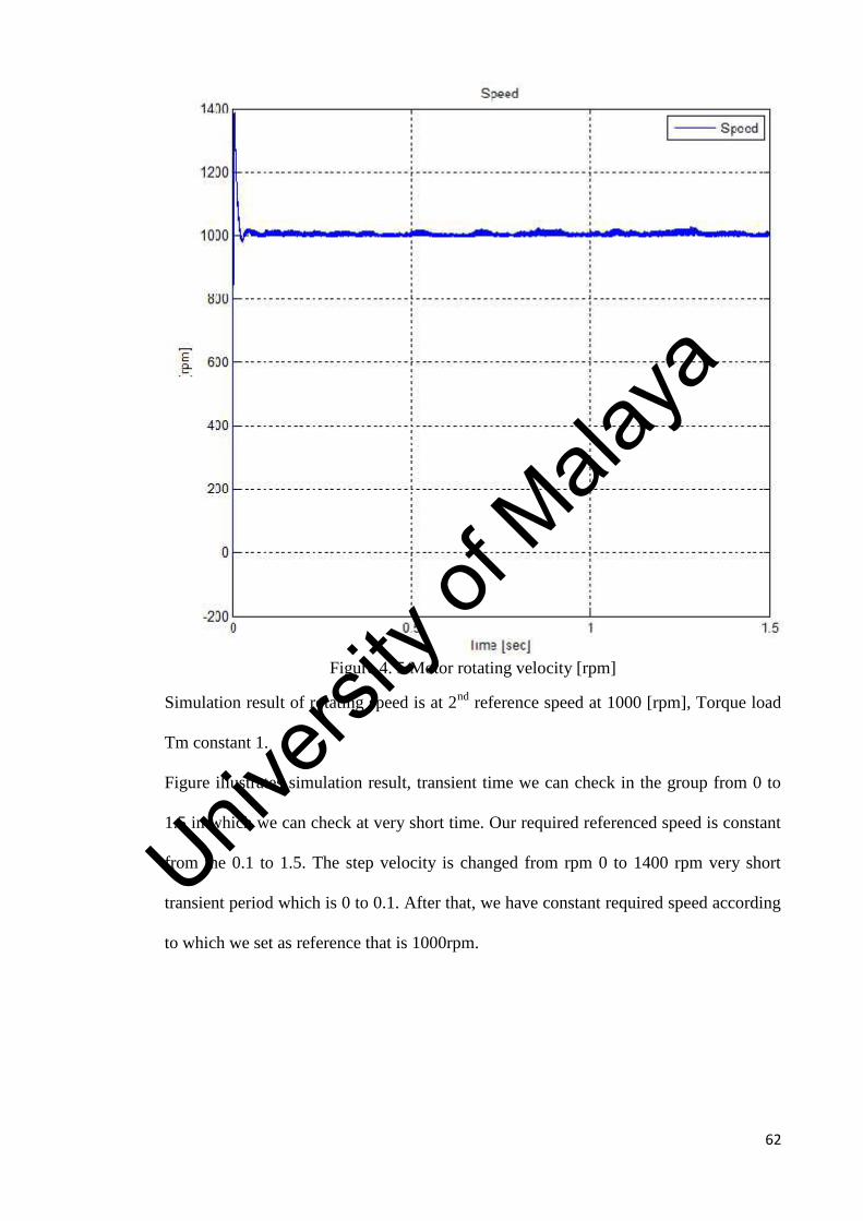
Figure 4. 5 Motor rotating velocity [rpm]
Simulation result of rotating speed is at 2nd reference speed at 1000 [rpm], Torque load
Tm constant 1.
Figure illustrates simulation result, transient time we can check in the group from 0 to
1.5 in which we can check at very short time. Our required referenced speed is constant
from the 0.1 to 1.5. The step velocity is changed from rpm 0 to 1400 rpm very short
transient period which is 0 to 0.1. After that, we have constant required speed according
to which we set as reference that is 1000rpm.
Univers
ity of
Mala
ya
63
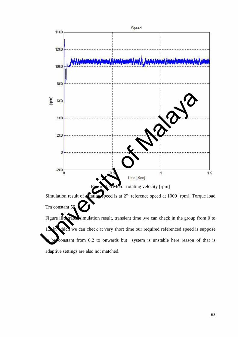
Figure 4. 6 Motor rotating velocity [rpm]
Simulation result of rotating speed is at 2nd reference speed at 1000 [rpm], Torque load
Tm constant 50.
Figure illustrates simulation result, transient time ,we can check in the group from 0 to
1.5 in which we can check at very short time our required referenced speed is suppose
to be constant from 0.2 to onwards but system is unstable here reason of that is
adaptive settings are also not matched.Univ
ersity
of M
alaya
64
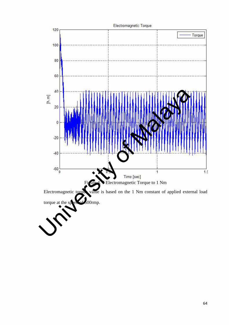
Figure 4. 7 Electromagnetic Torque to 1 Nm
Electromagnetic torque value is based on the 1 Nm constant of applied external load
torque at the speed of 500rmp.
Univers
ity of
Mala
ya
65
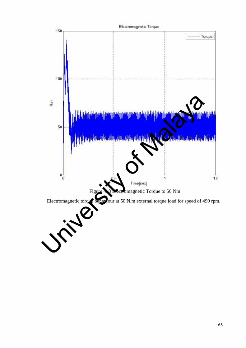
Figure 4. 8 Electromagnetic Torque to 50 Nm
Electromagnetic torque behaviour at 50 N.m external torque load for speed of 490 rpm.
Univers
ity of
Mala
ya
66
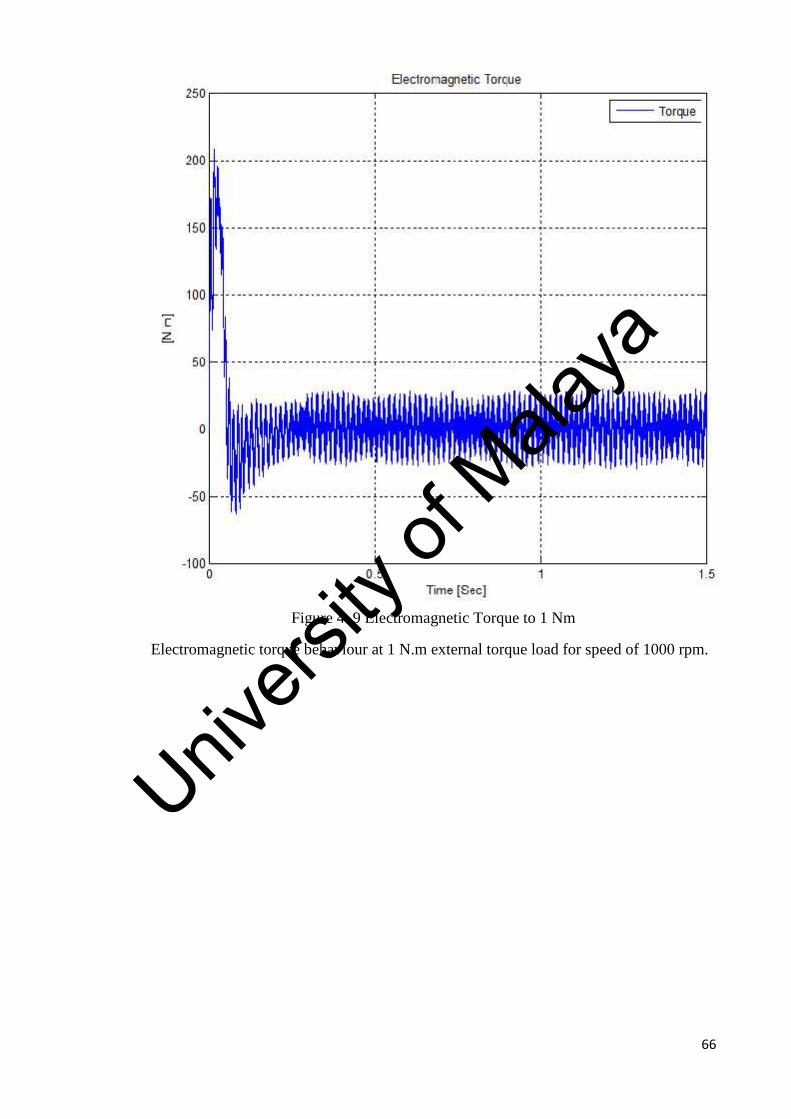
Figure 4. 9 Electromagnetic Torque to 1 Nm
Electromagnetic torque behaviour at 1 N.m external torque load for speed of 1000 rpm.
Univers
ity of
Mala
ya
67
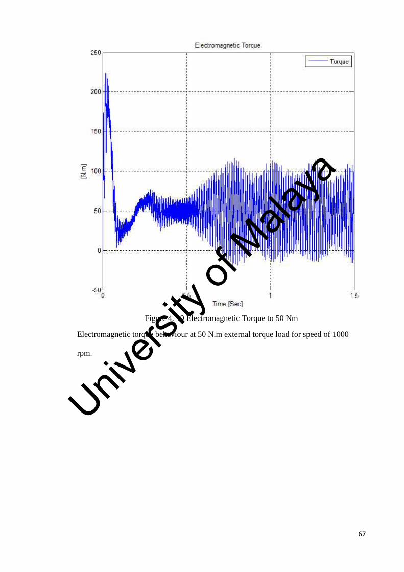
Figure 4. 10 Electromagnetic Torque to 50 Nm
Electromagnetic torque behaviour at 50 N.m external torque load for speed of 1000
rpm.
Univers
ity of
Mala
ya
68
4.1 Discussion of results
Adaptive observer scheme is tested on different values of external load torque, and the
reference speeds. From tested results in Matlab simulink, it gives the best result of
Electromagnetic torque on the value of external load torque 50Nm with the reference
speed of 490rpm which is constant at very low transient. Higher speed up to 1000rpm is
also tested on which external load 1 Nm gives also good result of speed which is stable
also at very low transient time.
System is configured at the speed starts from 490 [rpm] to [1000rpm] with external load
form 1 [Nm] to 50 [Nm]. Results as per required speed can achieved at required external
torque; for that there is need of change in variations parameter of induction motor,
adaptive flux until the system becomes stable. For adaptive observer it is confirmed
from the results that for getting the value which is required are depending on the
accurate parameters variations. As speed 490rpm is stable on external load 50 N.m, 0.96
flux value; any variation in other parameters of induction motor will make the system
disable. Any required speed with respect to external load using adaptive observer can be
attained by adjusting the parameter of induction motor until the system becomes stable.
Univers
ity of
Mala
ya
69
CHAPTER FIVE: CONCLUSION AND RECOMENDATION
5.1 Conclusion
The design and analysis of adaptive observer for controlling the performance of
induction motor has been presented. Different types of sensorless techniques were
discussed and reviewed together with the adaptive observer technique. The objective of
reviewing all techniques was to arrange the speed sensorless method techniques along
with the importance of merits and demerits for each method. The comparison between
different estimation of speed methods based on devised set of criteria was also
introduced. Mostly the exchanges which occur are between the simplicity regarding
implementation and the behaviour of over all system. Nevertheless, for the justification
of the certain scheme regarding specific applications from the results of each method is
considered a useful tool and all techniques are considered yet as powerful according to
the needs of specific requirements for the system.
For low speed procedure there is a need of introducing low speed application technique
such as; the technique of frequency signal injection method and rotor slot harmonic
methods, system which have high noise; mostly Extended Kalman Filter (EKF) is
preferable, due to noise reason EKF is designed as like in which can perform most
it is required to remove the chattering problems from the system. Artificial Intelligence
technique has the problem of complexity and the large time in computation although it
also demonstrates the better results.
Adaptive flux observer technique is presented in new way, as improved technique for
the induction motor, based on the correction of the value of the stator resistance and the
estimation of the load torque. The estimation of the torque is based on the use of the
error between real and estimated speed of induction motor, this will have to improve the
performances of the adaptive flux observer. The results show that the proposed adaptive
Univers
ity of
Mala
ya
70
observer offers better performances while tracking the speed and the flux, even in
presence of stator resistance variation.
5.2 Recommendation
As there are advantages and disadvantages of sensorless techniques, due to that all
techniques are important for specific application purpose; none of them would be
discarded for any disadvantage reason, all are useful. For example as Artificial
Intelligence (AI) system has better results but has problem of computation time and
complexity. However, AI techniques using with adaptive observer criteria can make
system more stable. It is highly recommended idea which comes after review of all
sensorless technique that by using the advantages of all sensorless techniques according
to needs such as; variation to parameters , configure system according to requirement ,
reduce complexity and try to reduce disadvantages for making the system more reliable
and accurate. Such adaptive observer scheme is preferred and possible by using
combination of techniques, SMO technique together with AI can give better results just
by eliminating chattering problem from SMO and reduce the complexity and
computation time of AI system together with variation in parameters.
Univers
ity of
Mala
ya
71
REFERENCES
Abdalla, T. Y., et al. (2010). Direct torque control system for a three phase inductionmotor with fuzzy logic based speed Controller. Energy, Power and Control (EPC-IQ),2010 1st International Conference on.
Abu-Rub, H. and J. Guzinski (2011). Simple observer for induction motor speedsensorless control. IECON 2011 - 37th Annual Conference on IEEE IndustrialElectronics Society.
Al-Tayie, J. K. and P. P. Acarnley (1997). "Estimation of speed, stator temperature androtor temperature in cage induction motor drive using the extended Kalman filteralgorithm." Electric Power Applications, IEE Proceedings - 144(5): 301-309.
Alamir, M. (2002). "Sensitivity analysis in simultaneous state/parameter estimation forinduction motors." Int. J. of Control 75(n°10): pp.753-758.
Campbell, J. and M. Sumner (2002). "Practical sensorless induction motor driveemploying an artificial neural network for online parameter adaptation." Electric PowerApplications, IEE Proceedings - 149(4): 255-260.
Consoli, A., et al. (2004). "Slip-frequency detection for indirect field-oriented controldrives." Industry Applications, IEEE Transactions on 40(1): 194-201.
Consoli, A., et al. (2004). "Speed- and current-sensorless field-oriented induction motordrive operating at low stator frequencies." Industry Applications, IEEE Transactions on40(1): 186-193.
da Silva, E. R. and M. D. Kankam (1997). Speed sensorless induction motor drives forelectrical actuators: schemes, trends and tradeoffs. Aerospace and ElectronicsConference, 1997. NAECON 1997., Proceedings of the IEEE 1997 National.
Derdiyok, A. (2005). "Speed-Sensorless Control of Induction Motor Using aContinuous Control Approach of Sliding-Mode and Flux Observer." IndustrialElectronics, IEEE Transactions on 52(4): 1170-1176.
Dr.JBV Subrahmanyam, T. S., TC Subramanyam,PK Sahoo,P Sankar (2011)."APPLICATION OF VECTOR CONTROL TECHNIQUE TO AC MOTORS." IJAERVol. No. 2(Issue No. V).
Edelbaher, G., et al. (2006). "Low-speed sensorless control of induction Machine."Industrial Electronics, IEEE Transactions on 53(1): 120-129.
Elloumi, M., et al. (1998). Survey of speed sensorless controls for IM drives. IndustrialElectronics Society, 1998. IECON '98. Proceedings of the 24th Annual Conference ofthe IEEE.
Univers
ity of
Mala
ya
72
Garcia Soto, G., et al. (1999). "Reduced-order observers for rotor flux, rotor resistanceand speed estimation for vector controlled induction motor drives using the extendedKalman filter technique." Electric Power Applications, IEE Proceedings - 146(3): 282-288.
Hinkkanen, M., et al. (2005). "Flux observer enhanced with low-frequency signalinjection allowing sensorless zero-frequency operation of induction motors." IndustryApplications, IEEE Transactions on 41(1): 52-59.
Holtz, J. (2002). "Sensorless control of induction motor drives." Proceedings of theIEEE 90(8): 1359-1394.
Holtz, J. (2006). "Sensorless Control of Induction Machines—With or WithoutSignal Injection?" Industrial Electronics, IEEE Transactions on 53(1): 7-30.
Holtz, J. and Q. Juntao (2002). "Sensorless vector control of induction motors at verylow speed using a nonlinear inverter model and parameter identification." IndustryApplications, IEEE Transactions on 38(4): 1087-1095.
Holtz, J. and Q. Juntao (2003). "Drift- and parameter-compensated flux estimator forpersistent zero-stator-frequency operation of sensorless-controlled induction motors."Industry Applications, IEEE Transactions on 39(4): 1052-1060.
Hossein Madadi Kojabadia, a. L. C. (2005). "Comparative study of pole placementmethods in adaptive flux observers." Control Engineering Practice Elsevier, 13: pp.749–757.
Huang, M. S. and C. M. Liaw (2003). "Improved field-weakening control for IFOinduction motor." Aerospace and Electronic Systems, IEEE Transactions on 39(2): 647-659.
Ilas, C., et al. (1994). Comparison of different schemes without shaft sensors for fieldoriented control drives. Industrial Electronics, Control and Instrumentation, 1994.IECON '94., 20th International Conference on.
J.P. Caron, J. P. H. (1995). "Modeling and Control of Induction Machine. TechnipEdition."
Jingchuan, L., et al. (2005). "An adaptive sliding-mode observer for induction motorsensorless speed control." Industry Applications, IEEE Transactions on 41(4): 1039-1046.
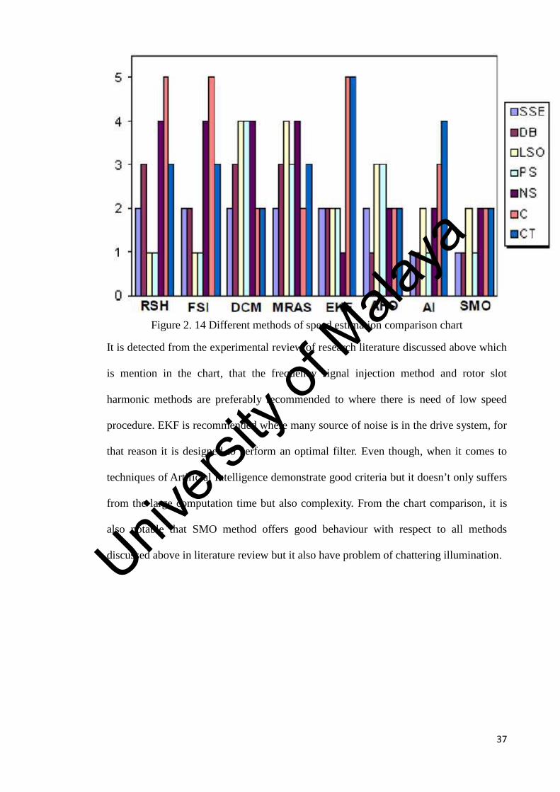
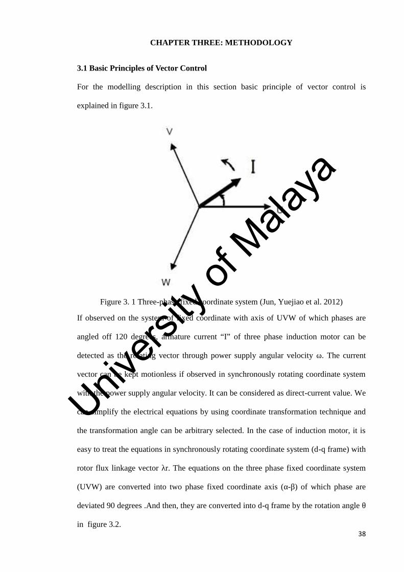
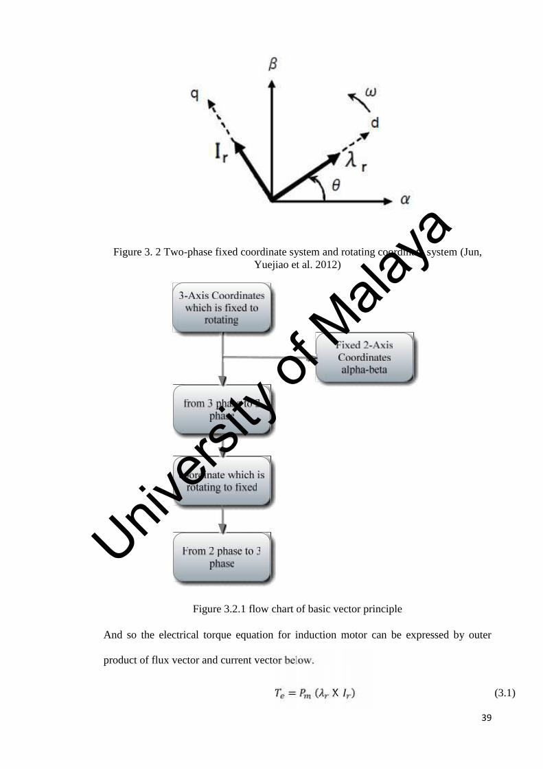
Jun, R., et al. (2012). Modeling and simulation of vector control system forasynchronous motor. Electronic System-Integration Technology Conference (ESTC),2012 4th.
Univers
ity of
Mala
ya
73
Khalil, H. K., et al. (2009). "Speed Observer and Reduced Nonlinear Model forSensorless Control of Induction Motors." Control Systems Technology, IEEETransactions on 17(2): 327-339.
Khan, M. R. and A. Iqbal (2012). Model reference adaptive system with simplesensorless flux observer for induction motor drive: MRAS with simple sensorless fluxobserver for induction motor drive. Power Electronics, Drives and Energy Systems(PEDES), 2012 IEEE International Conference on.
Khater, M. M., et al. (2006). A comparative study of sliding mode and Model ReferenceAdaptive Speed observers for induction motor drives. Power Systems Conference,2006. MEPCON 2006. Eleventh International Middle East.
kojabadi, M. (2005). "Simulation and experimental studies of model reference adaptivesystem for sensorless induction motor drive." Simulation Modeling practice and theory,Elsevier: pp. 451–464.
Korlinchak, C. and M. Comanescu (2012). "Sensorless field orientation of an inductionmotor drive using a time-varying observer." Electric Power Applications, IET 6(6): 353-361.
Lascu, C. and G. Andreescu (2006). "Sliding-mode observer and improved integratorwith DC-offset compensation for flux estimation in sensorless-controlled inductionmotors." Industrial Electronics, IEEE Transactions on 53(3): 785-794.
Lesan, A. Y. E., et al. (2012). Comparative study of speed estimation techniques forsensorless vector control of induction machine. IECON 2012 - 38th Annual Conferenceon IEEE Industrial Electronics Society.
Levi, E. and W. Mingyu (2002). "A speed estimator for high performance sensorlesscontrol of induction motors in the field weakening region." Power Electronics, IEEETransactions on 17(3): 365-378.
Levi, E. and W. Mingyu (2003). "Online identification of the mutual inductance forvector controlled induction motor drives." Energy Conversion, IEEE Transactions on18(2): 299-305.
Liu, J. and X. Wang (2008). Adaptive stator and rotor resistance identification forinduction machine without rotational transducer. Control Conference, 2008. CCC 2008.27th Chinese.
Lopez, J. C., et al. (2006). "Novel Fuzzy Adaptive Sensorless Induction Motor Drive."Industrial Electronics, IEEE Transactions on 53(4): 1170-1178.
Univers
ity of
Mala
ya
74
M. Alexandru , R. B., G. Ghelardi, S.M.Tenconi (2002). "An AC motor closed loopperformances with different rotor flux observers.MCFA Annals, Vol III, pp.1-3.".
M.S. ZAKY, M. K., H. YASIN and S.S. SHOKRALLA (2008). "Speed-SensorlessControl of Induction Motor Drives (Review Paper)." Volume 49.
Marwali, M. N. and A. Keyhani (1997). A comparative study of rotor flux based MRASand back EMF based MRAS speed estimators for speed sensorless vector control ofinduction machines. Industry Applications Conference, 1997. Thirty-Second IASAnnual Meeting, IAS '97., Conference Record of the 1997 IEEE.
Myoung-Ho, S. and H. Dong-Seok (2003). "Speed sensorless stator flux-orientedcontrol of induction machine in the field weakening region." Power Electronics, IEEETransactions on 18(2): 580-586.
Qilian, L. and J. M. Mendel (2000). "Interval type-2 fuzzy logic systems: theory anddesign." Fuzzy Systems, IEEE Transactions on 8(5): 535-550.
Rafiq, M. A., et al. (2012). Artificial Neural Network based speed tracking of a fieldoriented induction motor drive. Electrical & Computer Engineering (ICECE), 2012 7thInternational Conference on.
Rahman, M. F., et al. (2003). "A direct torque-controlled interior permanent-magnetsynchronous motor drive without a speed sensor." Energy Conversion, IEEETransactions on 18(1): 17-22.
Rashed, M. and A. F. Stronach (2004). "A stable back-EMF MRAS-based sensorlesslow-speed induction motor drive insensitive to stator resistance variation." ElectricPower Applications, IEE Proceedings - 151(6): 685-693.
Ravi Teja, A. V., et al. (2012). "A New Model Reference Adaptive Controller for FourQuadrant Vector Controlled Induction Motor Drives." Industrial Electronics, IEEETransactions on 59(10): 3757-3767.
Sangsefidi, Y., et al. (2012). A simple and low-cost method for three-phase inductionmotor control in high-speed applications. Power Electronics and Drive SystemsTechnology (PEDSTC), 2012 3rd.
Savoia, A., et al. (2012). Adaptive flux observer for induction machines with on-lineestimation of stator and rotor resistances. Power Electronics and Motion ControlConference (EPE/PEMC), 2012 15th International.
Schauder, C. (1992). "Adaptive speed identification for vector control of inductionmotors without rotational transducers." Industry Applications, IEEE Transactions on28(5): 1054-1061.
Univers
ity of
Mala
ya
75
Sedhuraman, K., et al. (2012). Comparison of learning algorithms for neural networkbased speed estimator in sensorless induction motor drives. Advances in Engineering,Science and Management (ICAESM), 2012 International Conference on.
Seong-Hwan, K., et al. (2001). "Speed-sensorless vector control of an induction motorusing neural network speed estimation." Industrial Electronics, IEEE Transactions on48(3): 609-614.
Sheng-Ming, Y. and K. Shuenn-Jenn (2000). "Performance evaluation of a velocityobserver for accurate velocity estimation of servo motor drives." Industry Applications,IEEE Transactions on 36(1): 98-104.
Siddique, A., et al. (2003). Applications of artificial intelligence techniques forinduction machine stator fault diagnostics: review. Diagnostics for Electric Machines,Power Electronics and Drives, 2003. SDEMPED 2003. 4th IEEE InternationalSymposium on.
Smidl, V. and Z. Peroutka (2012). "Advantages of Square-Root Extended Kalman Filterfor Sensorless Control of AC Drives." Industrial Electronics, IEEE Transactions on59(11): 4189-4196.
Staines, C. S., et al. (2006). "Sensorless control of induction Machines at zero and lowfrequency using zero sequence currents." Industrial Electronics, IEEE Transactions on53(1): 195-206.
Sun, K. and Y. Zhao (2010). A speed observer for speed sensorless control of inductionmotor. Future Computer and Communication (ICFCC), 2010 2nd InternationalConference on.
Tae-Sung, K., et al. (2005). "Speed sensorless stator flux-oriented control of inductionmotor in the field weakening region using Luenberger observer." Power Electronics,IEEE Transactions on 20(4): 864-869.
Tajima, H., et al. (2000). Consideration about problems and solutions of speedestimation method and parameter tuning for speed sensorless vector control of inductionmotor drives. Industry Applications Conference, 2000. Conference Record of the 2000IEEE.
Tajjudin, M., et al. (2012). Simple PID tuning using relay perturbation with errorswitching. System Engineering and Technology (ICSET), 2012 InternationalConference on.
Tarek BENMILOUD, A. O. (2011). "Improved Adaptive Flux Observer of an InductionMotor with Stator Resistance Adaptation." PRZEGLĄD ELEKTROTECHNICZNY(Electrical Review), ISSN 0033-2097, R. 87 NR 9a/2011.
Univers
ity of
Mala
ya
76
Ugale, R. T., et al. (2012). A low cost fast data acquisition system for capturing electricmotor starting and dynamic load transients. Power Electronics, Drives and EnergySystems (PEDES), 2012 IEEE International Conference on.
Vasic, V., et al. (2003). "A stator resistance estimation scheme for speed sensorlessrotor flux oriented induction motor drives." Energy Conversion, IEEE Transactions on18(4): 476-483.
Venkataramana Naik, N. and S. P. Singh (2012). A novel type-2 fuzzy logic control ofinduction motor drive using Scalar Control. Power Electronics (IICPE), 2012 IEEE 5thIndia International Conference on.
Volat, M. A. O. a. C. (2000). "Simulation of a Direct Field-Oriented Controller for anInduction Motor Using Matlab/Simulink. Proceeding of the IASTED InternationalConference Modelling and Simulation - Pittsburgh, Pennsylvania, USA."
Wang, P., et al. (2010). Speed-sensorless direct torque control system of inductionmotor. Control and Decision Conference (CCDC), 2010 Chinese.
Wolbank, T. M., et al. (2000). Comparison of different winding schemes reference totheir application on speed sensorless control of induction machines. IndustrialElectronics Society, 2000. IECON 2000. 26th Annual Confjerence of the IEEE.
Zaky, M. S. (2012). "Stability Analysis of Speed and Stator Resistance Estimators forSensorless Induction Motor Drives." Industrial Electronics, IEEE Transactions on 59(2):858-870.
Zamora, J. L. and A. Garcia-Cerrada (2000). "Online estimation of the stator parametersin an induction motor using only voltage and current measurements." IndustryApplications, IEEE Transactions on 36(3): 805-816.


![DNT 126 Basic Computer Programming [Asas Pengaturcaraan ...portal.unimap.edu.my/portal/page/portal30/Lecture...hadapan sebelum anda memulakan peperiksaan ini.] This question paper](https://static.documents.pub/doc/80x56/611b16d1db385263f31b1167/dnt-126-basic-computer-programming-asas-pengaturcaraan-hadapan-sebelum.jpg)


