Page 1
CFD Modelling
Combustor
Master’s Thesis in Solid and
AMIR KHODABANDEH
Department of Applied Mechanics
Division of Fluid Dynamics
CHALMERS UNIVERSITY OF TECHNOLOGY
Göteborg, Sweden 2011
Master’s thesis 2011:47
Modelling of Generic Gas Turbine
Solid and Fluid Mechanics
MIR KHODABANDEH
Mechanics
ynamics
CHALMERS UNIVERSITY OF TECHNOLOGY
Turbine
Page 3
MASTER’S THESIS IN SOLID AND FLUID MECHANICS
CFD Modelling of Generic Gas Turbine Combustor
AMIR KHODABANDEH
Department of Applied Mechanics
Division of Fluid Dynamics
CHALMERS UNIVERSITY OF TECHNOLOGY
Göteborg, Sweden 2011
Page 4
CFD Modelling of Generic Gas Turbine Combustor
AMIR KHODABANDEH
© AMIR KHODABANDEH, 2011
Master’s Thesis 2011:47
ISSN 1652-8557
Department of Applied Mechanics
Division of Fluid Dynamics
Chalmers University of Technology
SE-412 96 Göteborg
Sweden
Telephone: + 46 (0)31-772 1000
Cover:
Velocity streamlines inside gas turbine combustor.
Chalmers Reproservice, Göteborg/ Department of Applied Mechanics
Göteborg, Sweden 2011
Page 5
I
CFD Modelling of Generic Gas Turbine Combustor
Master’s Thesis in Solid and Fluid Mechanics
AMIR KHODABANDEH
Department of Applied Mechanics
Division of Fluid Dynamics
Chalmers University of Technology
ABSTRACT
New computational methods are continuously developed in order to solve problems in
different engineering fields. One of these fields is gas turbines, where the challenge is
to make gas turbines more efficient and to reduce emissions that are bad for the
environment. One of the main parts of a gas turbine that can be improved is the
combustion chamber. In order to optimize the combustion chamber, both
experimental and numerical methods are called for. Numerical optimization implies
the necessity to model the most important phenomena in combustion chambers such
as turbulent swirling flow, chemical reactions, heat transfer, and so on. In this project
we try to design a simple yet accurate model, for a generic combustor of industrial
interest, that may be tested in a relatively short time and that yields reliable results. An
important topic is here to perform grid sensitivity studies to make sure that the model
yields mesh independent results. Another topic of interest is the choice of turbulence
model and how this choice affects the grid sensitivity. Heat transfer models are also
important to evaluate. Different turbulence models and heat transfer models done with
this generic geometry and results will be discussed. After this project we made a
model that is numerically reliable, mesh independent and fast.
Key words:
Computational Fluid Dynamics, CFD, Gas turbine, Combustion chamber, Grid study,
Convection, Conduction.
Page 7
CHALMERS, Applied Mechanics, Master’s Thesis 2011:47 III
Table of contents
ABSTRACT I
TABLE OF CONTENTS III
PREFACE V
NOTATIONS AND ABBREVIATIONS VI
1 INTRODUCTION 1
1.1 Gas turbine 1
1.2 Gas turbine components 2
1.3 Combustion Chamber 3
2 THESIS DESCRIPTION 5
2.1 Aim of project 5
2.2 Software 5
2.3 Limitation 5
3 CALCULATION METHODOLOGY 7
3.1 Geometry Simplifications 7
3.2 Grid generation 8
3.3 Boundary conditions 10
3.4 Governing equations 10
3.4.1 Continuity equation 10
3.4.2 Momentum equation 11
3.4.3 Energy equation 11
3.4.4 Species equation 11
3.5 Turbulence models 11
3.5.1 k-ε Turbulence model 11
3.5.2 k-ω SST Turbulence model 12
3.6 Combustion models 13
3.6.1 Westbrook-Dryer one–step model 14
3.6.2 Westbrook-Dryer two-step model 14
3.7 Combustion-Turbulence interaction models 14
3.7.1 Eddy Dissipation Model 15
3.7.2 Finite Rate and Eddy Dissipation 15
3.8 Flow solution 15
3.8.1 Time stepping 15
3.8.2 Heat transfer 15
3.8.3 Turbulence 15
3.8.4 Combustion model 16
3.9 Convergence criteria 16
Page 8
CHALMERS, Applied Mechanics, Master’s Thesis 2011:47 IV
4 RESULTS AND POST PROCESSING 17
4.1 Case one 17
4.1.1 Temperature 18
4.1.2 Recirculation zones 18
4.1.3 CH4 Mass fraction 19
4.1.4 CO Mass fraction 20
4.1.5 Profile study 20
4.1.6 Tables 23
4.1.7 Result discussion 23
4.2 Case two 24
4.2.1 Temperature 24
4.2.2 Recirculation zones 25
4.2.3 CH4 Mass fraction 26
4.2.4 CO Mass fraction 26
4.2.5 Profile study 27
4.2.6 Tables 29
5 TURBULENCE AND HEAT TRANSFER MODEL STUDY 31
5.1 Software limitation for thin wall interface 31
5.2 Case three 31
5.2.1 Temperature 32
5.2.2 Recirculation zones 32
5.2.3 CH4 Mass fraction 33
5.2.4 CO Mass fraction 34
5.2.5 Profile study 34
5.2.6 Table 38
5.3 Results and Discussion 38
6 CONCLUSION 39
6.1 Future works 39
7 REFERENCES 41
7.1 Picture references 41
8 APPENDIX 43
8.1 Pictures 43
8.2 Heat transfer coefficient calculation 43
Page 9
CHALMERS, Applied Mechanics, Master’s Thesis 2011:47 V
Preface
In this study, numerical simulation of generic gas turbine combustor chamber has
been studied. The study has been carried out from August 2010 to September 2011.
The project is carried out at the department of Applied Mechanics, division of Fluid
dynamics, Chalmers University of Technology, Sweden. The thesis was done under
supervision of Lic. Eng. Abdallah Abou-Taouk and Professor Lars-Erik Eriksson. All
the calculations have been carried out at C3SE, Chalmers Centre for Computational
Science and Engineering, Chalmers University of Technology, Sweden.
Foremost, I would like to express my sincere gratitude to my supervisors Prof. Lars
Erik Eriksson and Lic. Eng. Abdallah Abou-Taouk for the continuous support of my
Master thesis, for their patience, motivations, enthusiasm, immense knowledge and
their valuable feedbacks on the report. Their guidance helped during the research and
writing of this thesis. I could not have imagined having this thesis finished without
their support.
My deepest gratitude goes to my family for their unflagging love and support
throughout my life; this dissertation is simply impossible without them. I am indebted
to my father, Hamid agho, for his care and love. I cannot ask for more from my
mother, maman Janet, as she is simply perfect. I have no suitable word that can fully
describe her everlasting love to me. I feel proud of my big brother, Khosrow kako, for
his talents. He had been a role model for me to follow unconsciously when I was a
teenager and has always been one of my best counsellors.
Göteborg September 2011
Amir Khodabandeh
Page 10
CHALMERS, Applied Mechanics, Master’s Thesis 2011:47 VI
Notations and abbreviations
Roman upper case letters
��� First constant in ε equation
��� Second constant in ε equation
CFD Computational Fluid Dynamics
D Diffusion coefficient
Fi Force vector (ith
component)
NOx generic term for the mono-nitrogen oxides NO and NO2
��� Strain rate tensor
Roman lower case letters
c Concentration
h Convective heat transfer coefficient
� Turbulence kinetic energy
t time
u Velocity vector
Greek upper case letters
∅ Blend factor
Greek lower case letters
∗ Constant in k- ω model
�j
��
ε Dissipation of turbulent kinetic energy
σij Cauchy stress tensor
ρ Density
�� Kinematic eddy viscosity
ω Specific dissipation
Page 11
CHALMERS, Applied Mechanics, Master’s Thesis 2011:47 1
1 Introduction
1.1 Gas turbine
Energy is needed in order to make machines work. One of the best forms of energy is
electrical energy. It can be carried over distances and can be produced almost
anywhere with proper tools. There are several devices that produce electrical energy
such as solar panels, wind turbines and gas turbines. In this project we will focus on
gas turbines. Gas turbines produce electrical energy from burning a combustible
mixture of fuel (e.g. natural gas or evaporated hydrocarbons) and air. When the gas
mixture burns, the volume of the gas will increase. This expansion in gas volume
makes a rotor of a turbine rotate and this rotation may then be converted to electrical
energy.
There are two important families of gas turbines:
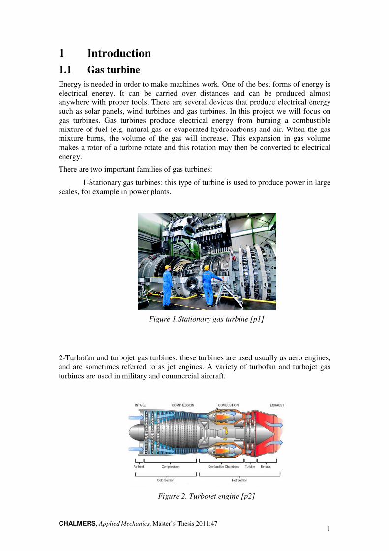
1-Stationary gas turbines: this type of turbine is used to produce power in large
scales, for example in power plants.
Figure 1.Stationary gas turbine [p1]
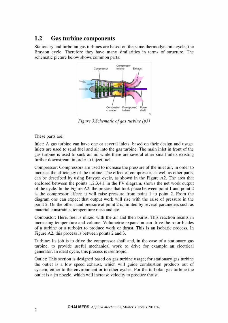
2-Turbofan and turbojet gas turbines: these turbines are used usually as aero engines,
and are sometimes referred to as jet engines. A variety of turbofan and turbojet gas
turbines are used in military and commercial aircraft.
Figure 2. Turbojet engine [p2]
Page 12
CHALMERS, Applied Mechanics, Master’s Thesis 2011:47 2
1.2 Gas turbine components
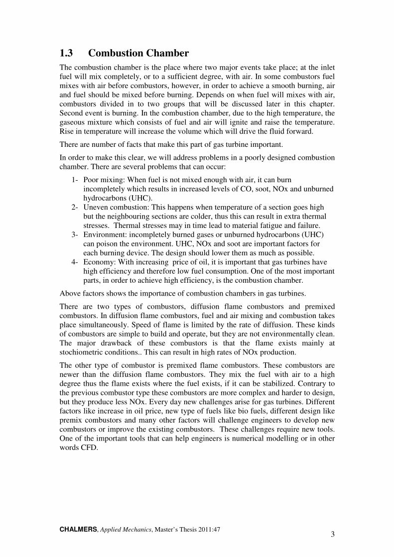
Stationary and turbofan gas turbines are based on the same thermodynamic cycle; the
Brayton cycle. Therefore they have many similarities in terms of structure. The
schematic picture below shows common parts:
Figure 3.Schematic of gas turbine [p3]
These parts are:
Inlet: A gas turbine can have one or several inlets, based on their design and usage.
Inlets are used to send fuel and air into the gas turbine. The main inlet in front of the
gas turbine is used to suck air in; while there are several other small inlets existing
further downstream in order to inject fuel.
Compressor: Compressors are used to increase the pressure of the inlet air, in order to
increase the efficiency of the turbine. The effect of compressor, as well as other parts,
can be described by using Brayton cycle, as shown in the Figure A2. The area that
enclosed between the points 1,2,3,4,1 in the PV diagram, shows the net work output
of the cycle. In the Figure A2, the process that took place between point 1 and point 2
is the compressor effect; it will raise pressure from point 1 to point 2. From the
diagram one can expect that output work will rise with the raise of pressure in the
point 2. On the other hand pressure at point 2 is limited by several parameters such as
material constraints, temperature raise and etc.
Combustor: Here, fuel is mixed with the air and then burns. This reaction results in
increasing temperature and volume. Volumetric expansion can drive the rotor blades
of a turbine or a turbojet to produce work or thrust. This is an isobaric process. In
Figure A2, this process is between points 2 and 3.
Turbine: Its job is to drive the compressor shaft and, in the case of a stationary gas
turbine, to provide useful mechanical work to drive for example an electrical
generator. In ideal cycle, this process is isentropic.
Outlet: This section is designed based on gas turbine usage; for stationary gas turbine
the outlet is a low speed exhaust, which will guide combustion products out of
system, either to the environment or to other cycles. For the turbofan gas turbine the
outlet is a jet nozzle, which will increase velocity to produce thrust.
Page 13
CHALMERS, Applied Mechanics, Master’s Thesis 2011:47 3
1.3 Combustion Chamber
The combustion chamber is the place where two major events take place; at the inlet
fuel will mix completely, or to a sufficient degree, with air. In some combustors fuel
mixes with air before combustors, however, in order to achieve a smooth burning, air
and fuel should be mixed before burning. Depends on when fuel will mixes with air,
combustors divided in to two groups that will be discussed later in this chapter.
Second event is burning. In the combustion chamber, due to the high temperature, the
gaseous mixture which consists of fuel and air will ignite and raise the temperature.
Rise in temperature will increase the volume which will drive the fluid forward.
There are number of facts that make this part of gas turbine important.
In order to make this clear, we will address problems in a poorly designed combustion
chamber. There are several problems that can occur:
1- Poor mixing: When fuel is not mixed enough with air, it can burn
incompletely which results in increased levels of CO, soot, NOx and unburned
hydrocarbons (UHC).
2- Uneven combustion: This happens when temperature of a section goes high
but the neighbouring sections are colder, thus this can result in extra thermal
stresses. Thermal stresses may in time lead to material fatigue and failure.
3- Environment: incompletely burned gases or unburned hydrocarbons (UHC)
can poison the environment. UHC, NOx and soot are important factors for
each burning device. The design should lower them as much as possible.
4- Economy: With increasing price of oil, it is important that gas turbines have
high efficiency and therefore low fuel consumption. One of the most important
parts, in order to achieve high efficiency, is the combustion chamber.
Above factors shows the importance of combustion chambers in gas turbines.
There are two types of combustors, diffusion flame combustors and premixed
combustors. In diffusion flame combustors, fuel and air mixing and combustion takes
place simultaneously. Speed of flame is limited by the rate of diffusion. These kinds
of combustors are simple to build and operate, but they are not environmentally clean.
The major drawback of these combustors is that the flame exists mainly at
stochiometric conditions.. This can result in high rates of NOx production.
The other type of combustor is premixed flame combustors. These combustors are
newer than the diffusion flame combustors. They mix the fuel with air to a high
degree thus the flame exists where the fuel exists, if it can be stabilized. Contrary to
the previous combustor type these combustors are more complex and harder to design,
but they produce less NOx. Every day new challenges arise for gas turbines. Different
factors like increase in oil price, new type of fuels like bio fuels, different design like
premix combustors and many other factors will challenge engineers to develop new
combustors or improve the existing combustors. These challenges require new tools.
One of the important tools that can help engineers is numerical modelling or in other
words CFD.
Page 14
CHALMERS, Applied Mechanics, Master’s Thesis 2011:47 4
Page 15
CHALMERS, Applied Mechanics, Master’s Thesis 2011:47 5
2 Thesis description
2.1 Aim of project
• The main focus of this project is to do a grid study for a characteristic gas
turbine combustion chamber.
• Using different turbulence models on a characteristic gas turbine combustion
chamber.
• Modelling the convective and conductive heat transfer of the casing with the
ambient.
2.2 Software
In this project three software packages were used.
1- ICEMCFD: This software is used to draw the surface geometry. Then it used
again in order to mesh the computational domain which is bounded by the surface
geometry.
2- CFX: This is the solver software. This software is used to simulate the flow in the
computational domain. Also some part of the post processing is carried with
CFXpost
3- Matlab: It is used together with CFXpost to post process the results, plot charts
etc.
2.3 Limitation
The time frame of this project was 1 year, so the chosen geometry could not be too
complex (further detail on this part will be discussed on geometry section).
Calculations took place on the local Linux cluster BEDA, with 8 processors. Each
simulation needed about 9 days of wall clock time.
The design of geometry was done on a desktop computer. Due to the limited project
time the grid generation work had to be minimized and therefore the combustor
geometry had to be simplified.
Page 16
CHALMERS, Applied Mechanics, Master’s Thesis 2011:47 6
Page 17
CHALMERS, Applied Mechanics, Master’s Thesis 2011:47 7
3 Calculation methodology
3.1 Geometry Simplifications
The simplifications that were done are the following:
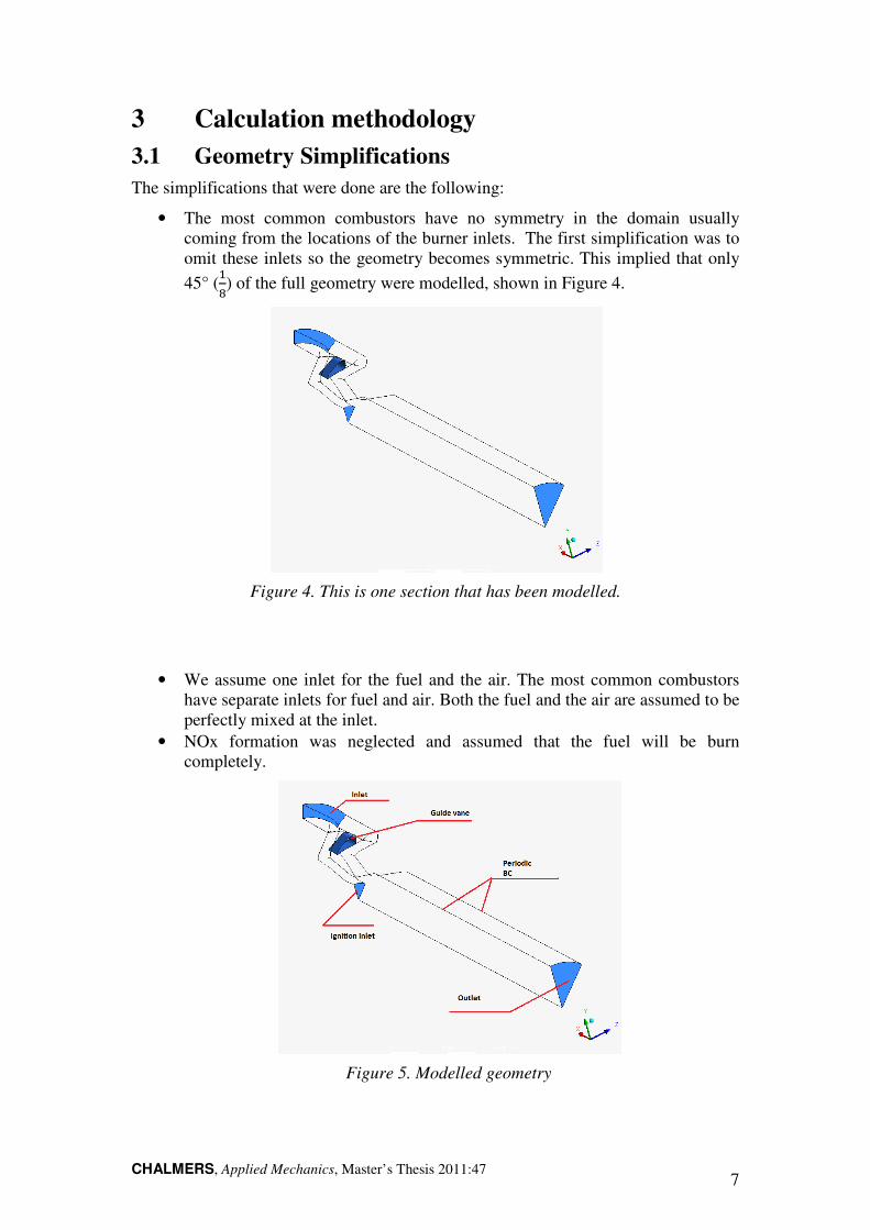
• The most common combustors have no symmetry in the domain usually
coming from the locations of the burner inlets. The first simplification was to
omit these inlets so the geometry becomes symmetric. This implied that only
45° (��) of the full geometry were modelled, shown in Figure 4.
Figure 4. This is one section that has been modelled.
• We assume one inlet for the fuel and the air. The most common combustors
have separate inlets for fuel and air. Both the fuel and the air are assumed to be
perfectly mixed at the inlet.
• NOx formation was neglected and assumed that the fuel will be burn
completely.
Figure 5. Modelled geometry
Page 18
CHALMERS8
The simplified geometry consists of an inlet, a guide vane and
bottom faces are set to walls, while the side faces are axial symmetric
shown in Figure 5.
There is a secondary inlet
in the beginning of the iteration process
the mass flow rate is set to zero
The full geometry is shown in
3.2 Grid generation
Four different mesh sizes were investigated in the present work. These
400,000 or 400K, 500,000 or 500K, 1
section consists of a vane, which is shown in
Figure
In Figure 7, three sections are shown. In
colour with the name of “Free slip wall” or “ramp”. This section
from other walls, because of strange interaction of k
free slip wall contrary to other walls.
CHALMERS, Applied Mechanics, Master’s Thesis 2011:47
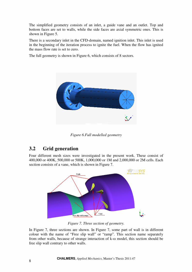
The simplified geometry consists of an inlet, a guide vane and an outlet. Top and
walls, while the side faces are axial symmetric
in the CFD-domain, named ignition inlet. This
iteration process to ignite the fuel. When the flow has ignited
set to zero.
shown in Figure 6, which consists of 8 sectors.
Figure 6.Full modelled geometry
Grid generation
Four different mesh sizes were investigated in the present work. These
000 or 500K, 1,000,000 or 1M and 2,000,000 or 2M cells.
of a vane, which is shown in Figure 7.
Figure 7. Three section of geometry.
7, three sections are shown. In Figure 7, some part of wall is in different
colour with the name of “Free slip wall” or “ramp”. This section name
walls, because of strange interaction of k-ω model, this section should be
contrary to other walls.
outlet. Top and
walls, while the side faces are axial symmetric ones. This is
ignition inlet. This inlet is used
. When the flow has ignited
Four different mesh sizes were investigated in the present work. These consist of
000 or 2M cells. Each
7, some part of wall is in different
name separately
del, this section should be
Page 19
CHALMERS, Applied Mechanics, Master’s Thesis 2011:47 9
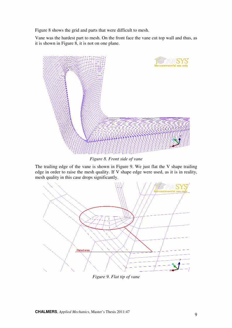
Figure 8 shows the grid and parts that were difficult to mesh.
Vane was the hardest part to mesh. On the front face the vane cut top wall and thus, as
it is shown in Figure 8, it is not on one plane.
Figure 8. Front side of vane
The trailing edge of the vane is shown in Figure 9. We just flat the V shape trailing
edge in order to raise the mesh quality. If V shape edge were used, as it is in reality,
mesh quality in this case drops significantly.
Figure 9. Flat tip of vane
Page 20
CHALMERS, Applied Mechanics, Master’s Thesis 2011:47 10
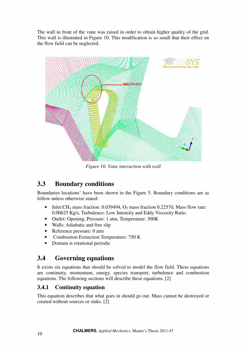
The wall in front of the vane was raised in order to obtain higher quality of the grid.
This wall is illustrated in Figure 10. This modification is so small that their effect on
the flow field can be neglected.
Figure 10. Vane interaction with wall
3.3 Boundary conditions
Boundaries locations’ have been shown in the Figure 5. Boundary conditions are as
follow unless otherwise stated:
• Inlet:CH4 mass fraction: 0.039494, O2 mass fraction 0.22570, Mass flow rate:
0.00625 Kg/s, Turbulence: Low Intensity and Eddy Viscosity Ratio.
• Outlet: Opening, Pressure: 1 atm, Temperature: 300K
• Walls: Adiabatic and free slip
• Reference pressure: 0 atm
• Combustion Extinction Temperature: 750 K
• Domain is rotational periodic
3.4 Governing equations
It exists six equations that should be solved to model the flow field. These equations
are continuity, momentum, energy, species transport, turbulence and combustion
equations. The following sections will describe these equations. [2]
3.4.1 Continuity equation
This equation describes that what goes in should go out. Mass cannot be destroyed or
created without sources or sinks. [2]
Page 21
CHALMERS, Applied Mechanics, Master’s Thesis 2011:47 11
This equation reads: ���� + ∇. ���� = 0 ��.
3.4.2 Momentum equation
Momentum is a vector quantity that is product of mass by velocity vector. In a closed
system, momentum cannot be created nor destroyed. It should be conserved. The
equation reads: [2]
��!�� + "� = 0 ��. #
3.4.3 Energy equation
Energy equation describes that in a closed system, energy cannot be created nor
destroyed. This equation is solved during the simulation to compute temperature field.
We chose total energy for this equation which will be discussed in solver section. [2]
3.4.4 Species equation
Species equation, like the previous equations, describes that species in a closed
systems, cannot be created or destroyed.
This equation reads as follows:
�$�� + �∇c = &∇�c ��. '
3.5 Turbulence models
3.5.1 k-ε Turbulence model
In the following section, turbulence and combustions models are discussed more in
details, due to their importance.
The k-ε model is one of the most common turbulence models. It is a two equation
model which means that two extra transport equations is included to represent the
turbulent properties of the flow. This allows the two equation model to account for
history effects like convection and diffusion of turbulent energy.
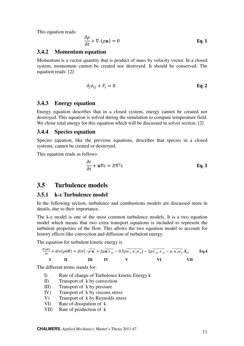
The equation for turbulent kinetic energy is
�()� * + +,-���.� = +,-/−1′�′22222 + 24�′5′672222222 − 0.5�9′6. 9′69′722222222222: − 245′67. 5′67222222222 − �. 9′69′722222222. ��� Eq.4
I II III IV V VI VII
The different terms stands for:
I) Rate of change of Turbulence kinetic Energy k
II) Transport of k by convection
III) Transport of k by pressure
IV) Transport of k by viscous stress
V) Transport of k by Reynolds stress
VI) Rate of dissipation of k
VII) Rate of production of k
Page 22
CHALMERS, Applied Mechanics, Master’s Thesis 2011:47 12
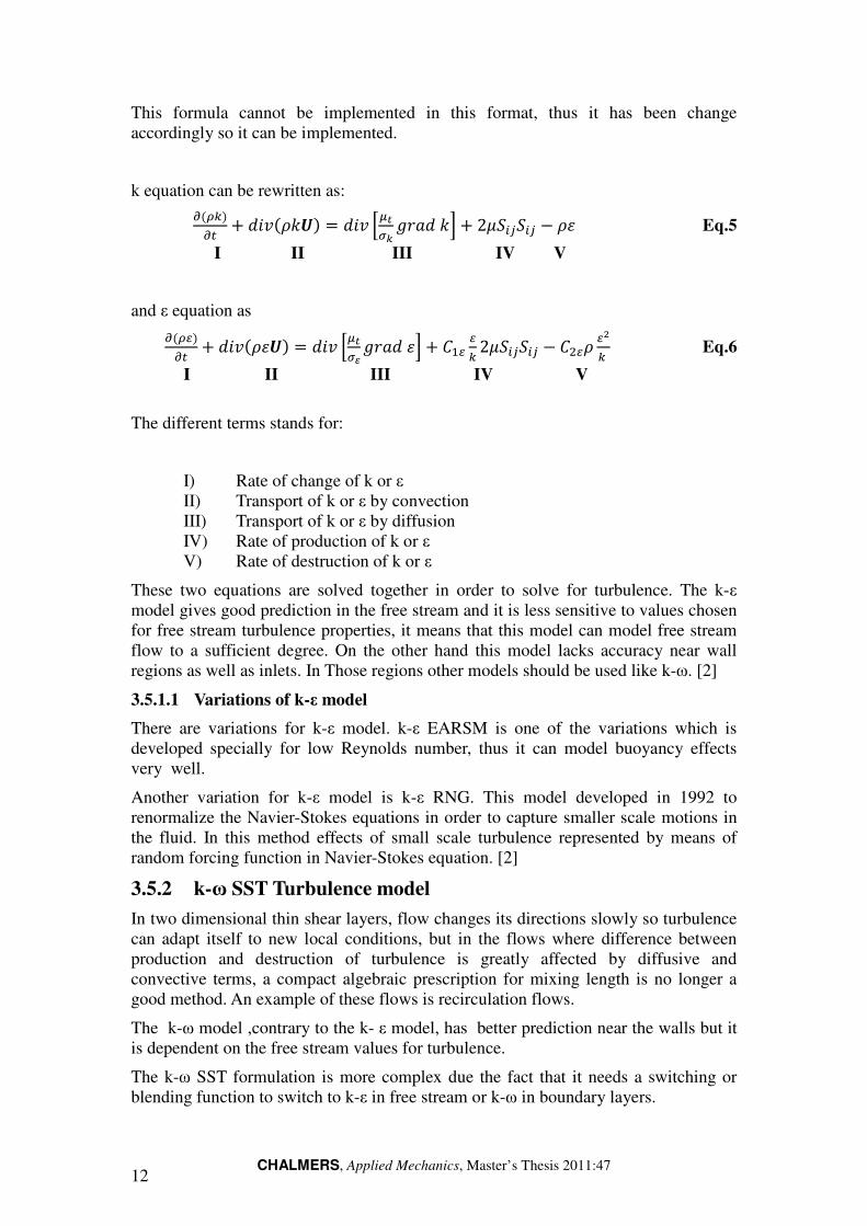
This formula cannot be implemented in this format, thus it has been change
accordingly so it can be implemented.
k equation can be rewritten as:
�()� * + +,-���.� = +,- ;<=>? @AB+ �C + 24D��D�� − �E Eq.5
I II III IV V
and ε equation as
�(�� * + +,-��E.� = +,- ;<=>F @AB+ EC + ��� �
) 24D��D�� − ���� �G) Eq.6
I II III IV V
The different terms stands for:
I) Rate of change of k or ε
II) Transport of k or ε by convection
III) Transport of k or ε by diffusion
IV) Rate of production of k or ε
V) Rate of destruction of k or ε
These two equations are solved together in order to solve for turbulence. The k-ε
model gives good prediction in the free stream and it is less sensitive to values chosen
for free stream turbulence properties, it means that this model can model free stream
flow to a sufficient degree. On the other hand this model lacks accuracy near wall
regions as well as inlets. In Those regions other models should be used like k-ω. [2]
3.5.1.1 Variations of k-ε model
There are variations for k-ε model. k-ε EARSM is one of the variations which is
developed specially for low Reynolds number, thus it can model buoyancy effects
very well.
Another variation for k-ε model is k-ε RNG. This model developed in 1992 to
renormalize the Navier-Stokes equations in order to capture smaller scale motions in
the fluid. In this method effects of small scale turbulence represented by means of
random forcing function in Navier-Stokes equation. [2]
3.5.2 k-ω SST Turbulence model
In two dimensional thin shear layers, flow changes its directions slowly so turbulence
can adapt itself to new local conditions, but in the flows where difference between
production and destruction of turbulence is greatly affected by diffusive and
convective terms, a compact algebraic prescription for mixing length is no longer a
good method. An example of these flows is recirculation flows.
The k-ω model ,contrary to the k- ε model, has better prediction near the walls but it
is dependent on the free stream values for turbulence.
The k-ω SST formulation is more complex due the fact that it needs a switching or
blending function to switch to k-ε in free stream or k-ω in boundary layers.
Page 23
CHALMERS, Applied Mechanics, Master’s Thesis 2011:47 13
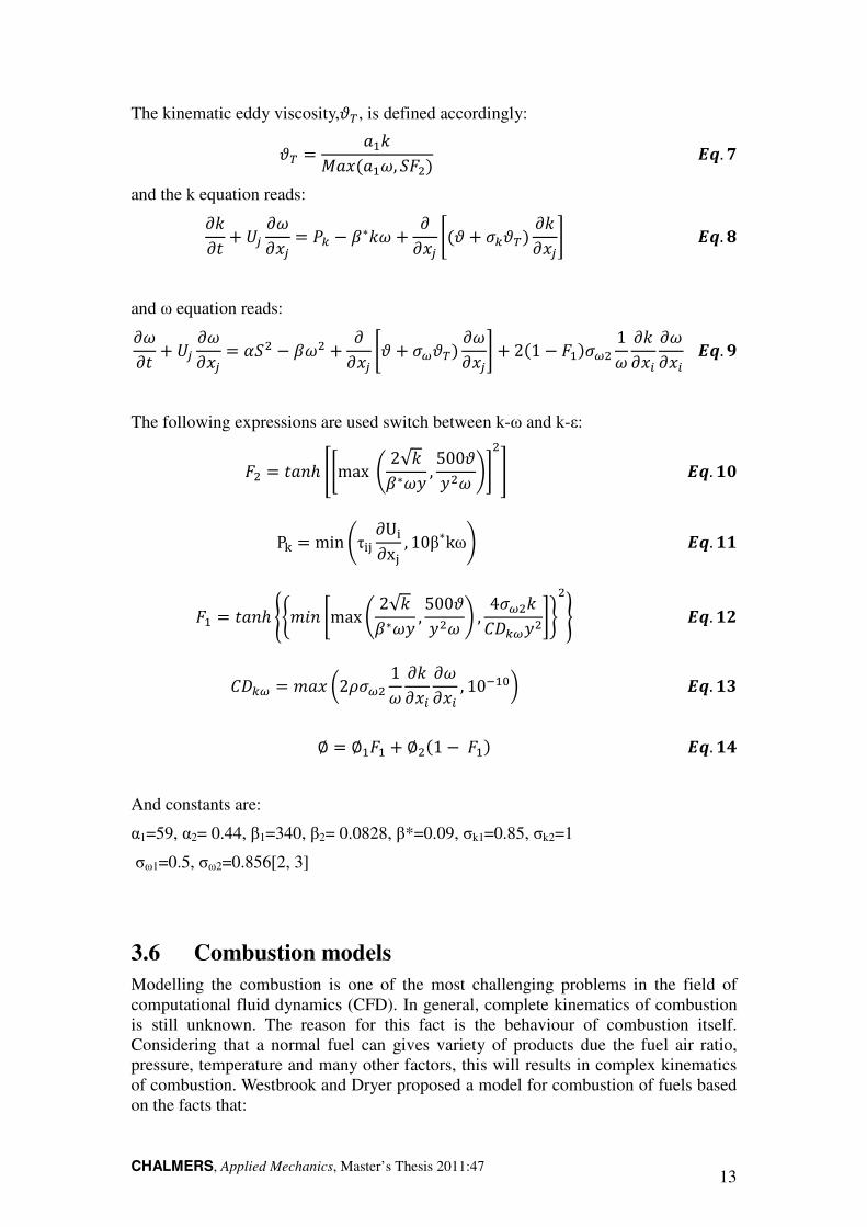
The kinematic eddy viscosity,��, is defined accordingly:
�� = B��HBI�B�J, D"�� LM. N
and the k equation reads:
���� + O� �J�I� = P) − ∗�J + ��I� Q�� + !)��� ���I�R LM. S
and ω equation reads:
�J�� + O� �J�I� = TD� − J� + ��I� Q� + !U��� �J�I�R + 2�1 − "��!U� 1J ���I��J�I� LM. W
The following expressions are used switch between k-ω and k-ε:
"� = �BXℎ ZQmax ^ 2√�∗J` , 500�`�J aR�
b LM. c
Pe = min ^τhi ∂Uh∂xi , 10β∗kωa LM.
"� = �BXℎ mno,X Qmax ^ 2√�∗J` , 500�`�J a , 4!U���&)U`�Rq�
r LM. #
�&)U = oBI s2�!U� 1J ���I��J�I� , 10t�uv LM. '
∅ = ∅�"� + ∅��1 − "�� LM. w
And constants are:
α1=59, α2= 0.44, β1=340, β2= 0.0828, β*=0.09, σk1=0.85, σk2=1
σω1=0.5, σω2=0.856[2, 3]
3.6 Combustion models
Modelling the combustion is one of the most challenging problems in the field of
computational fluid dynamics (CFD). In general, complete kinematics of combustion
is still unknown. The reason for this fact is the behaviour of combustion itself.
Considering that a normal fuel can gives variety of products due the fuel air ratio,
pressure, temperature and many other factors, this will results in complex kinematics
of combustion. Westbrook and Dryer proposed a model for combustion of fuels based
on the facts that:
Page 24
CHALMERS, Applied Mechanics, Master’s Thesis 2011:47 14
1- General detailed mechanism cannot be currently included in the most
multidimensional problems because of computer size, speed and cost
requirements.
2- Detailed mechanisms have been developed and validated for simplest fuel and
are not available for most practical fuels.
3- There are many occasions where the great amount of chemical information is
unnecessary and a simple two step model would be sufficient.
Westbrook and Dryer have developed two global reaction mechanisms, one-step and
two-step. [4,5]
3.6.1 Westbrook-Dryer one–step model
Due the simpler model, this model is faster comparing to two step models. This model
can be used where the combustion effects are small and fast results are needed. This
model also gives a good estimation of indicator of the expected temperature levels.
However, this model got several disadvantages. This model will overestimate Tad,
adiabatic temperature of flame. This overestimation will grow with increasing the
equivalence ratio, which is directly related to increased amount of CO and H2 in the
reaction products. Single step model also neglect the fact that hydro carbons are burn
in a somewhat sequential manner. This means that CO and H2 are not consumed
unless all the hydro carbon fuel is used.
The general formulation of this global reaction mechanism is: [6]
Fuel+O2→CO2+H2O Eq.15
3.6.2 Westbrook-Dryer two-step model
This model is based on two reactions. This results in one big advantage, the ability to
treat arbitrary fuels. This is valuable property which makes this model important;
however this model has disadvantages too. Two-step model is developed for shock
tube ignition delays which make this model not suitable to model flame speed or
reaction rate in plug flow or stirred reactors. This model also lacks accuracy to model
radical species, thus it does not have enough precision to model NOx formation.
Westbrook-Dryer model two-step model has been chosen since in this project NOx
formation is neglected and also the flow is not stirred flow.
The formulation for Methane in this model is as follows:
Reaction I: CH4+O2 → CO+ H2O Eq.16
Reaction II CO+0.5O2→CO2 Eq.17
As one sees, this is a general formulation which can model almost all kind of
hydrocarbon fuels. Westbrook and Dryer said that this model will also work for non-
hydrocarbon fuels but they didn’t test it.
3.7 Combustion-Turbulence interaction models
Two models are used in this project: Eddy Dissipation Model (EDM), Finite Rate and
Eddy Dissipation (FRED). These models are used to solve the interaction between
turbulence and combustion.
Page 25
CHALMERS, Applied Mechanics, Master’s Thesis 2011:47 15
3.7.1 Eddy Dissipation Model
The eddy dissipation combustion model (EDM) which derives from the eddy
dissipation concept is extended to simulate combustion within large eddy simulations
(LES).The reaction chemistry is a simple infinitely fast one step global irreversible
reaction. The model for the reaction rate is developed from a combination of local
kinetics modelling using an Arrhenius law and a new form of the EDC model adapted
for LES. The modelling can in principle be applied to both premixed and non-
premixed flame and can easily be extended for more complex chemistry. [8]
3.7.2 Finite Rate and Eddy Dissipation
Reaction rates are assumed to be controlled by the turbulence, so expensive Arrhenius
chemical kinetic calculations can be avoided. The model is computationally cheap but
for realistic results, only one or two step combustion model should be used. [6]
3.8 Flow solution
ANSYS CFX v12.1 was used as solver. The numerical settings for the solver are
described below.
3.8.1 Time stepping
The problem is solved as a steady state flow problem, consistent with the RANS
turbulence modelling used, which means that relatively large time steps are used in
order to achieve a converged solution as quickly as possible. In spite of the turbulence
model the flame itself is slightly unsteady, but the oscillations are negligible.
3.8.2 Heat transfer
“Total energy including viscous work terms” model is used, which means that the
total energy models the transport of enthalpy including the kinetic energy effects. This
model should be used where there is change in density or the Mach number exceeds
0.2; in both of these cases kinetic energy effects are significant. In ANSYS CFX,
when one chooses total energy the fluid is modelled as compressible, regardless of the
original fluid condition, i.e. gases with Mach number less than 0.2. One should know
that incompressible fluid does not exists in reality but for the gases with Mach number
less than 0.2 the compressible effects are in general negligible. [6]
3.8.3 Turbulence
For the turbulence both the k-ω SST and the k-ε turbulence models are used. The k-ε
model is one of the most common turbulence models. It is a two equation model that
includes two extra transport equations to represent the turbulent properties of the flow.
This allows the model to account for history effects like convection and diffusion of
turbulent energy.
The k-ε model has a good prediction in the free stream, but near the walls, the
prediction is poor since adverse pressure gradient is presented. This is not the case for
the k-ω which has a good accuracy close to the walls. Based on this idea Menter
(1992a) invent a model that called SST k-ω which uses a transformation of k-ε in to k-
ω near walls and k-ε model in the fully turbulent regions far from walls.
For wall treatment scalable wall function is used. Standard wall functions are based
on the assumption that the first grid point off the wall (or the first integration point) is
located in the universal law-of-the-wall or logarithmic region. This helps to have
Page 26
CHALMERS, Applied Mechanics, Master’s Thesis 2011:47 16
higher aspect ratios which means reduce density of mesh near the walls. This results
in lower computational costs but it will also reduce the accuracy because high aspect
ratio results in high round off errors. On the other hand, standard wall function
formulations are difficult to handle, because it should have high resolution near walls
means higher computational costs. Also if the resolution becomes too fine, the first
grid spacing can be too small to bridge the viscous sub layer. In this case, the
logarithmic profile assumptions are no longer satisfied. The user should make sure
that both upper and lower limit for the grid size are not crossed. Recently, alternative
formulations (scalable wall functions) have become available, Menter and Esch,
which allow for a systematic grid refinement when using wall functions. [7]
3.8.4 Combustion model
Westbrook-Dryer two-step model was used for combustion. This model is mainly
focused on the modelling of the combustion at temperatures above 1000K. At these
temperatures experimental data are usually hard to gather due the small time scales,
usually in the order of micro seconds, but on the other hand reactions simpler
formulations. This method is mainly used for hydrocarbon fuels at high temperatures,
however Westbrook and Dryer state that using the same method, one can develop
relations for other non-hydrocarbon fuels. [4]
3.9 Convergence criteria
In order to determine if convergence is obtained, residuals are constantly monitored
and when they are reasonable flatted out, after 10,000 iterations, the run is stopped
and the results are post-processed.
Page 27
CHALMERS, Applied Mechanics, Master’s Thesis 2011:47 17
4 Results and post processing
The grid sensitivity study was performed on four different mesh sizes, 400,000
(400K), 500,000(500K), 1,000,000 (1M) and 2,000,000 (2M) cells. The aim of this
study is to obtain a mesh size were the results are grid-independent. Furthermore, two
different turbulence models were used in the study, the k-ε and the k-ω SST model.
The comparisons were done considering the temperature, the pressure, the axial
velocity and the major species, CH4, CO2 and CO.
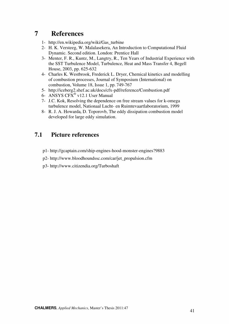
These properties are calculated on seven locations: mid plane, YZ, YZ1, YZ2, YZ3,
YZ4 and YZ.
Mid plane is the bisector of the burner chamber. The other planes are located in the
burner. To address the planes we use a dimensionless number as percent. it means how
far they are from the combustion chamber entry, 0% and 100% locations are shown in
the Figure A1,in the appendix section. The locations of the plane are as follows:
1- YZ @ 0.000%
2- YZ1 @ 3.846%
3- YZ2 @ 9.587%
4- YZ3 @ 18.197%
5- YZ 4 @ 26.808%
6- YZ 5 @ 41.159%
4.1 Case one
In this section we discussed the obtained results for different cases
The following cases are for the grid study, which means that all the settings are the,
but the number of cells is different. The following settings were used:
Turbulence: k-ε, wall function: scalable, heat transfer: total energy with viscous work
terms, combustion model: two-step model. Combustion-turbulence interaction model:
Eddy dissipation.
Page 28
CHALMERS18
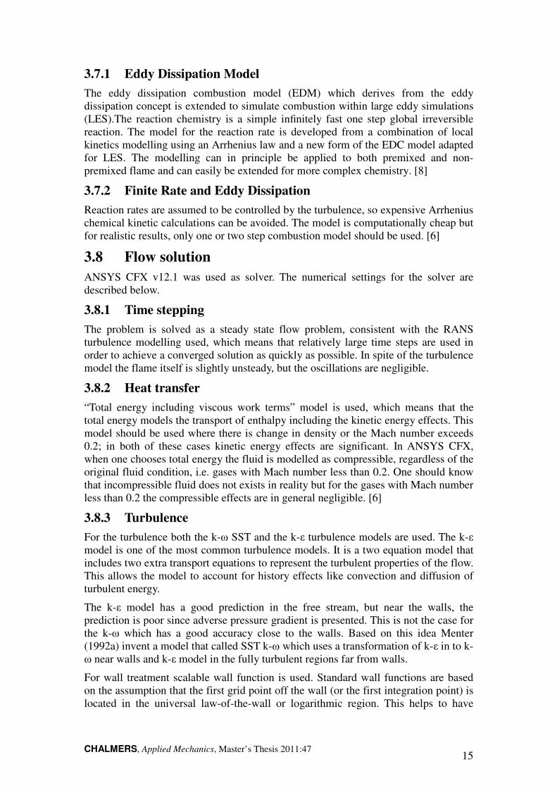
4.1.1 Temperature
The left column shows the
temperature at mid plane. From up to down: 400K, 500K, 1M and 2M
implies that the temperature results are independent of number of cells
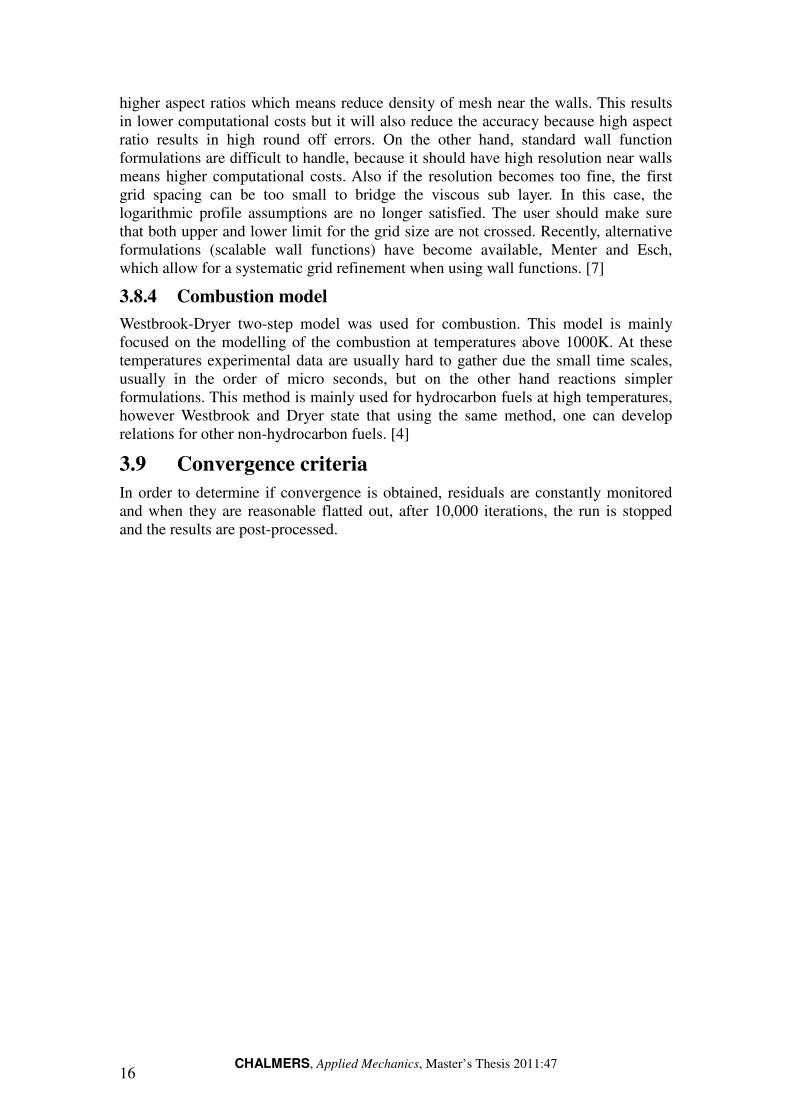
4.1.2 Recirculation
Figure 12 shows the recirculation zone inside the domain, which means that the axial
velocity is in opposite direction to the flow field.
(right); Bottom row: 1M (left) and 2M (right)
other. It implies that the recirculation zones are independent of number of cells. In
CHALMERS, Applied Mechanics, Master’s Thesis 2011:47
Figure 12. Temperature contours;
the temperature contours at YZ planes and the right
temperature at mid plane. From up to down: 400K, 500K, 1M and 2M
implies that the temperature results are independent of number of cells.
zones
Figure 13. Recirculation zones;
12 shows the recirculation zone inside the domain, which means that the axial
velocity is in opposite direction to the flow field. Top row: 400K (
Bottom row: 1M (left) and 2M (right). These regions look similar with each
other. It implies that the recirculation zones are independent of number of cells. In
he right side shows
temperature at mid plane. From up to down: 400K, 500K, 1M and 2M cells. This
.
12 shows the recirculation zone inside the domain, which means that the axial
400K (left) and 500K
These regions look similar with each
other. It implies that the recirculation zones are independent of number of cells. In
Page 29
CHALMERS, Applied Mechanics
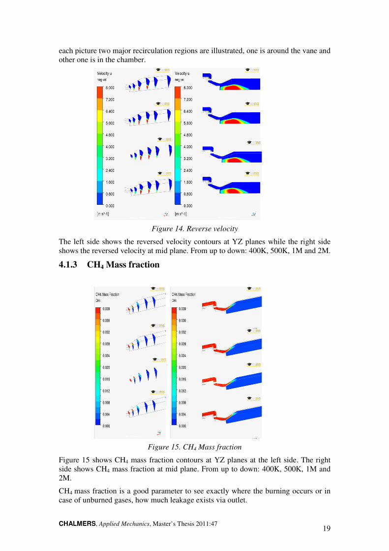
each picture two major recirculation region
other one is in the chamber.
The left side shows the reversed
shows the reversed velocity at mid plane. From up to down: 400K, 500K, 1M and 2M
4.1.3 CH4 Mass fraction
Figure 15 shows CH4 mass fraction contours at YZ planes
side shows CH4 mass fraction at mid plane. From up to down: 400K, 500K, 1M and
2M.
CH4 mass fraction is a good parameter to see exactly where the burning occurs or in
case of unburned gases, how much leakage exists via outlet.
Mechanics, Master’s Thesis 2011:47
each picture two major recirculation regions are illustrated, one is around the vane and
other one is in the chamber.
Figure 14. Reverse velocity
the reversed velocity contours at YZ planes while the right
velocity at mid plane. From up to down: 400K, 500K, 1M and 2M
Mass fraction
Figure 15. CH4 Mass fraction
mass fraction contours at YZ planes at the left side
mass fraction at mid plane. From up to down: 400K, 500K, 1M and
mass fraction is a good parameter to see exactly where the burning occurs or in
case of unburned gases, how much leakage exists via outlet.
19
illustrated, one is around the vane and
velocity contours at YZ planes while the right side
velocity at mid plane. From up to down: 400K, 500K, 1M and 2M.
at the left side. The right
mass fraction at mid plane. From up to down: 400K, 500K, 1M and
mass fraction is a good parameter to see exactly where the burning occurs or in
Page 30
CHALMERS20
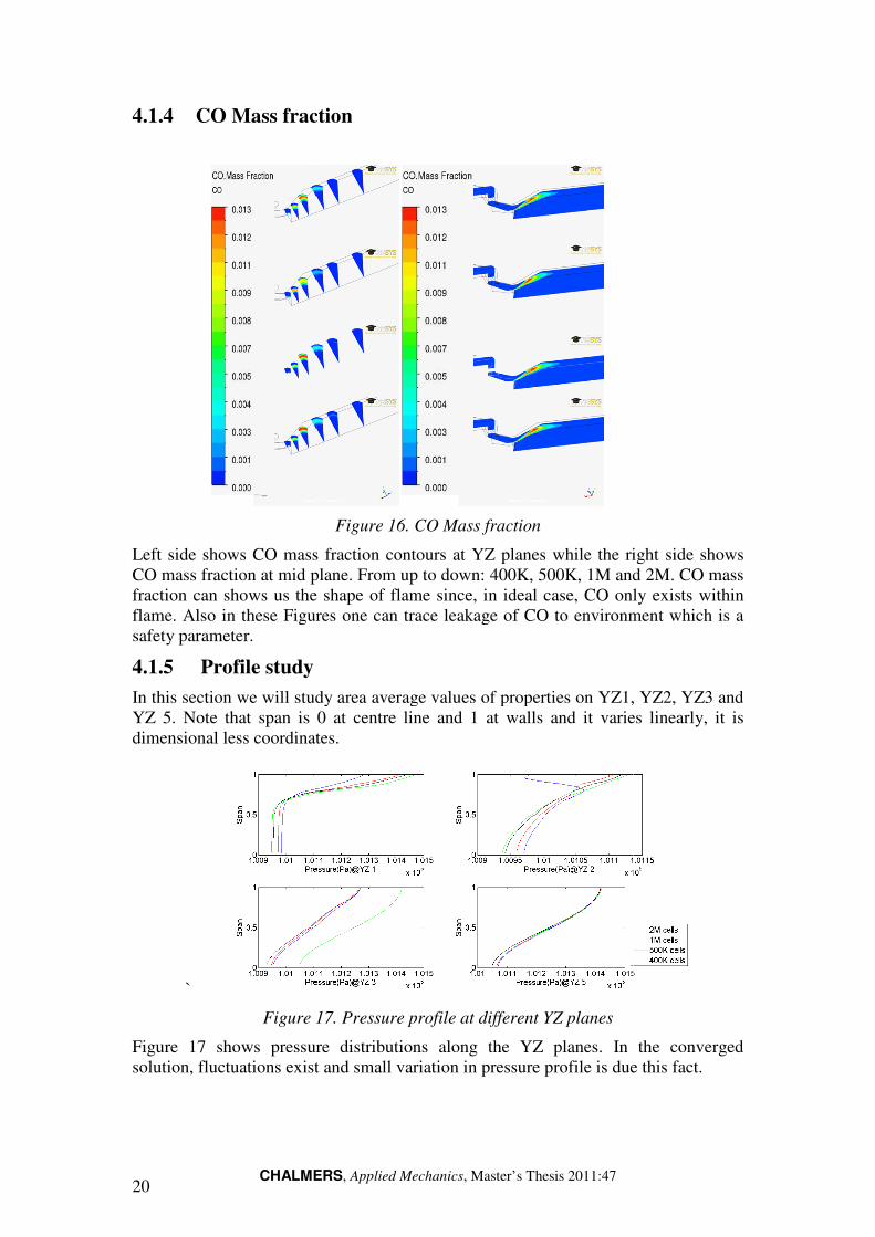
4.1.4 CO Mass fraction
Left side shows CO mass fraction contours at YZ planes while the right
CO mass fraction at mid plane. From up to down: 400K, 500K, 1M and 2M
fraction can shows us the shape of flame
flame. Also in these Figure
safety parameter.
4.1.5 Profile study
In this section we will study area aver
YZ 5. Note that span is 0 at
dimensional less coordinate
`
Figure 17. Pressure profile at different YZ planes
Figure 17 shows pressure
solution, fluctuations exist and small variation in pressure profile is due this fact.
CHALMERS, Applied Mechanics, Master’s Thesis 2011:47
fraction
Figure 16. CO Mass fraction
shows CO mass fraction contours at YZ planes while the right
CO mass fraction at mid plane. From up to down: 400K, 500K, 1M and 2M
fraction can shows us the shape of flame since, in ideal case, CO only exists within
Figures one can trace leakage of CO to environment which is a
In this section we will study area average values of properties on YZ1, YZ2, YZ3 and
YZ 5. Note that span is 0 at centre line and 1 at walls and it varies linearly, it is
dimensional less coordinates.
17. Pressure profile at different YZ planes
ressure distributions along the YZ planes. In the converged
, fluctuations exist and small variation in pressure profile is due this fact.
shows CO mass fraction contours at YZ planes while the right side shows
CO mass fraction at mid plane. From up to down: 400K, 500K, 1M and 2M. CO mass
in ideal case, CO only exists within
one can trace leakage of CO to environment which is a
age values of properties on YZ1, YZ2, YZ3 and
line and 1 at walls and it varies linearly, it is
along the YZ planes. In the converged
, fluctuations exist and small variation in pressure profile is due this fact.
Page 31
CHALMERS, Applied Mechanics, Master’s Thesis 2011:47 21
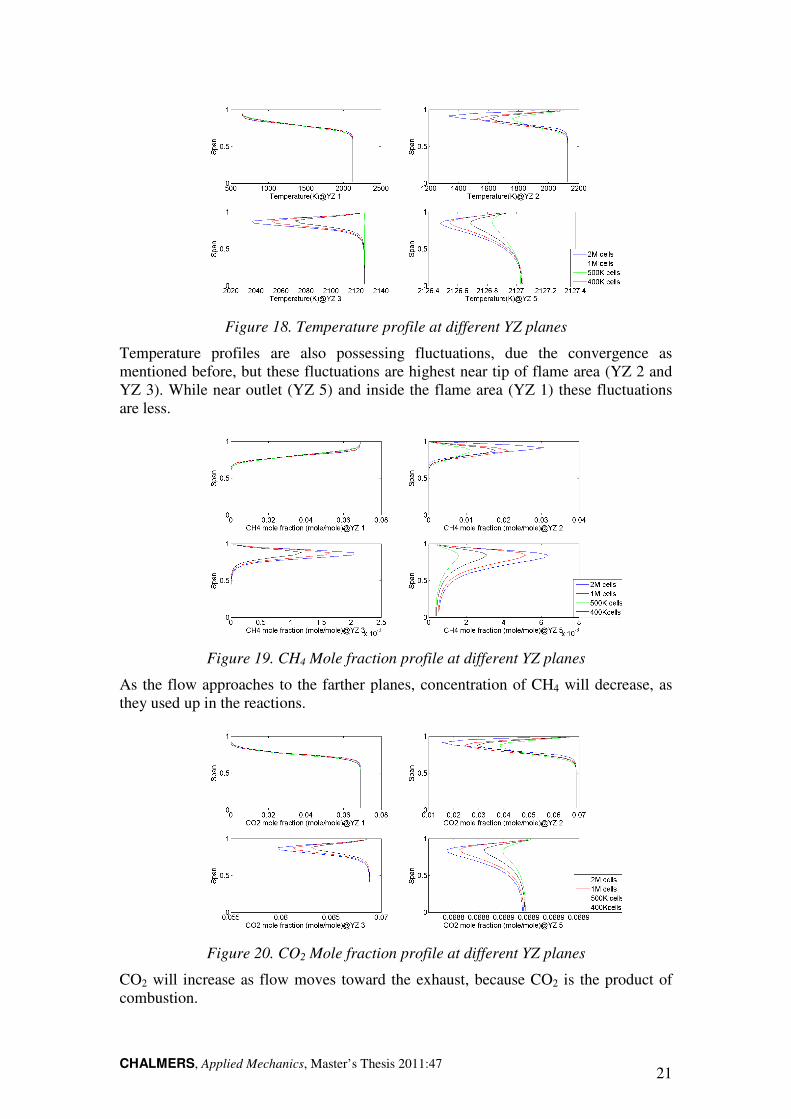
Figure 18. Temperature profile at different YZ planes
Temperature profiles are also possessing fluctuations, due the convergence as
mentioned before, but these fluctuations are highest near tip of flame area (YZ 2 and
YZ 3). While near outlet (YZ 5) and inside the flame area (YZ 1) these fluctuations
are less.
Figure 19. CH4 Mole fraction profile at different YZ planes
As the flow approaches to the farther planes, concentration of CH4 will decrease, as
they used up in the reactions.
Figure 20. CO2 Mole fraction profile at different YZ planes
CO2 will increase as flow moves toward the exhaust, because CO2 is the product of
combustion.
Page 32
CHALMERS, Applied Mechanics, Master’s Thesis 2011:47 22
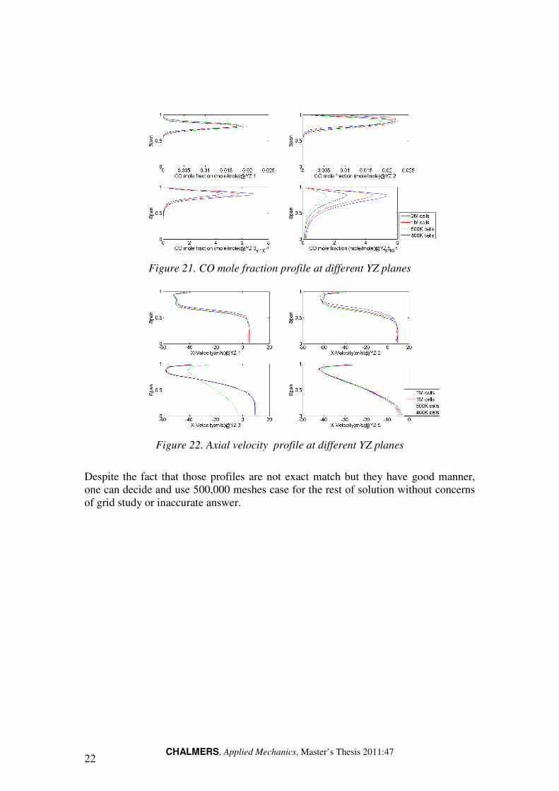
Figure 21. CO mole fraction profile at different YZ planes
Figure 22. Axial velocity profile at different YZ planes
Despite the fact that those profiles are not exact match but they have good manner,
one can decide and use 500,000 meshes case for the rest of solution without concerns
of grid study or inaccurate answer.
Page 33
CHALMERS, Applied Mechanics
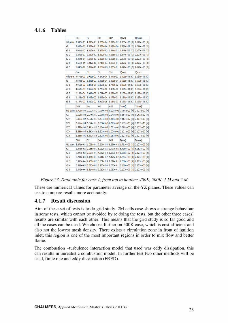
4.1.6 Tables
Figure 23 .Data table for case 1, f
These are numerical values for parameter average on the YZ planes. These values can
use to compare results more accurately
4.1.7 Result discussion
Aim of these set of tests is to do grid study. 2M cell
in some tests, which cannot be avoided
results are similar with each other
all the cases can be used. We choose further on 500K c
also not the lowest mesh density. There exists a circulation zone in front of ignition
inlet; this region is one of the most important regions in order to mix flow and better
flame.
The combustion –turbulence interaction
can results in unrealistic combustion model. In further test two other methods will be
used, finite rate and eddy dissipation (FRED).
Mechanics, Master’s Thesis 2011:47
23 .Data table for case 1, from top to bottom: 400K, 500K, 1 M and 2 M
These are numerical values for parameter average on the YZ planes. These values can
more accurately.
Result discussion
Aim of these set of tests is to do grid study. 2M cells case shows a strange behavio
, which cannot be avoided by re doing the tests, but the other three cases’
with each other. This means that the grid study is so far good and
all the cases can be used. We choose further on 500K case, which is cost efficient and
also not the lowest mesh density. There exists a circulation zone in front of ignition
inlet; this region is one of the most important regions in order to mix flow and better
turbulence interaction model that used was eddy dissipation
can results in unrealistic combustion model. In further test two other methods will be
used, finite rate and eddy dissipation (FRED).
23
500K, 1 M and 2 M
These are numerical values for parameter average on the YZ planes. These values can
a strange behaviour
re doing the tests, but the other three cases’
. This means that the grid study is so far good and
ase, which is cost efficient and
also not the lowest mesh density. There exists a circulation zone in front of ignition
inlet; this region is one of the most important regions in order to mix flow and better
eddy dissipation, this
can results in unrealistic combustion model. In further test two other methods will be
Page 34
CHALMERS24
4.2 Case two
This case is also a grid study which means we are going to study four different
meshes, but all have same solution setting.
Settings are:
Turbulence model: k-ω SST, Wall function: Automatic, Heat transfer: Total energy
with viscous work term, combustion model:
Boundary conditions are same except for the ramp part of the wall, which is se
slip in order to avoid strange numerical error and
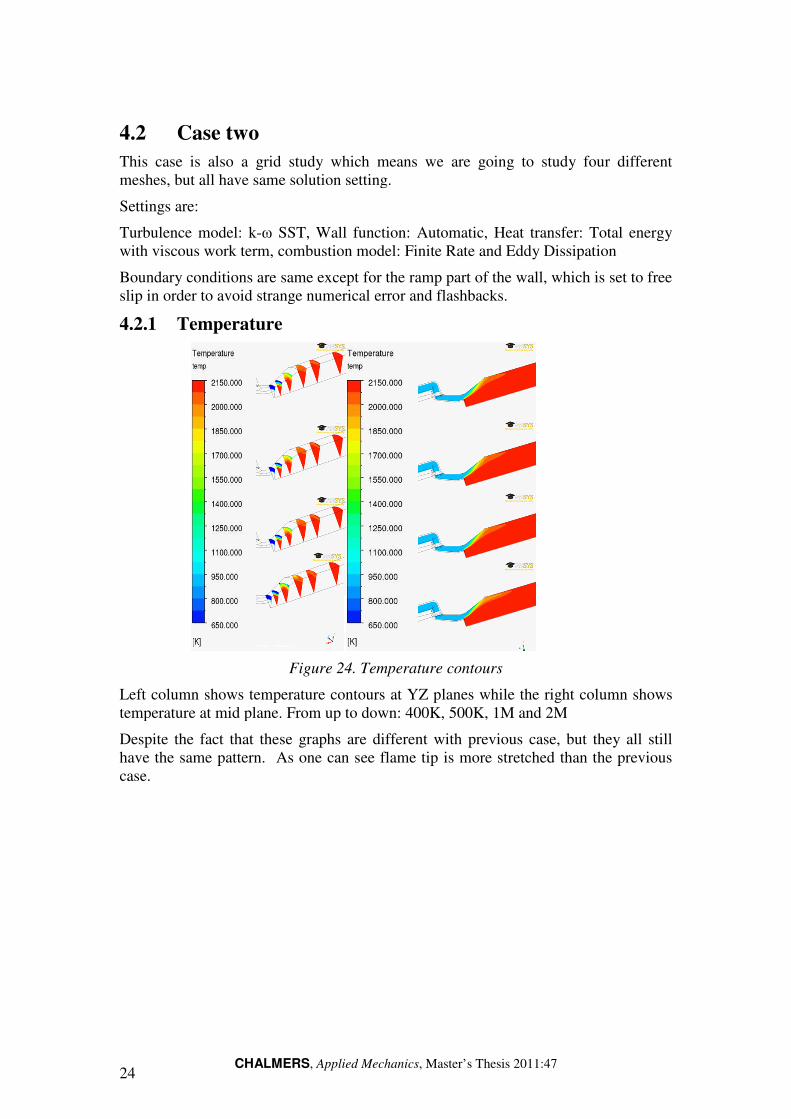
4.2.1 Temperature
Left column shows temperature
temperature at mid plane. From up to down: 400K, 500K, 1M and 2M
Despite the fact that these graphs are different with previous case, but they
have the same pattern. As one can see flame tip is more stretched
case.
CHALMERS, Applied Mechanics, Master’s Thesis 2011:47
This case is also a grid study which means we are going to study four different
meshes, but all have same solution setting.
ω SST, Wall function: Automatic, Heat transfer: Total energy
with viscous work term, combustion model: Finite Rate and Eddy Dissipation
Boundary conditions are same except for the ramp part of the wall, which is se
slip in order to avoid strange numerical error and flashbacks.
Temperature
Figure 24. Temperature contours
Left column shows temperature contours at YZ planes while the right column shows
temperature at mid plane. From up to down: 400K, 500K, 1M and 2M
Despite the fact that these graphs are different with previous case, but they
same pattern. As one can see flame tip is more stretched than the previous
This case is also a grid study which means we are going to study four different
SST, Wall function: Automatic, Heat transfer: Total energy
issipation
Boundary conditions are same except for the ramp part of the wall, which is set to free
planes while the right column shows
Despite the fact that these graphs are different with previous case, but they all still
than the previous
Page 35
CHALMERS, Applied Mechanics
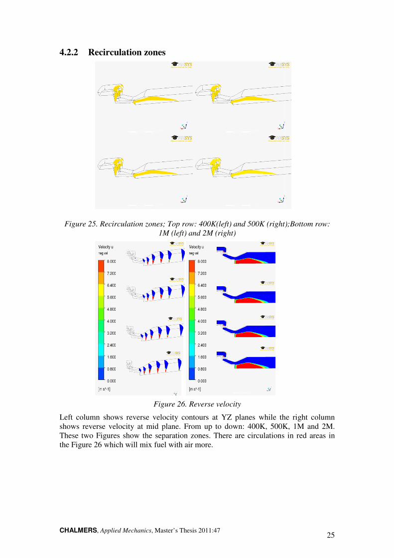
4.2.2 Recirculation zones
Figure 25. Recirculation
Left column shows reverse
shows reverse velocity at mid plane. From up to down: 400K, 500K, 1M and 2M
These two Figures show the separation zones.
the Figure 26 which will mix fuel with air more.
Mechanics, Master’s Thesis 2011:47
ecirculation zones
Recirculation zones; Top row: 400K(left) and 500K (right);Bottom row:
1M (left) and 2M (right)
Figure 26. Reverse velocity
reverse velocity contours at YZ planes while the right column
velocity at mid plane. From up to down: 400K, 500K, 1M and 2M
s show the separation zones. There are circulations
26 which will mix fuel with air more.
25
row: 400K(left) and 500K (right);Bottom row:
velocity contours at YZ planes while the right column
velocity at mid plane. From up to down: 400K, 500K, 1M and 2M.
in red areas in
Page 36
CHALMERS26
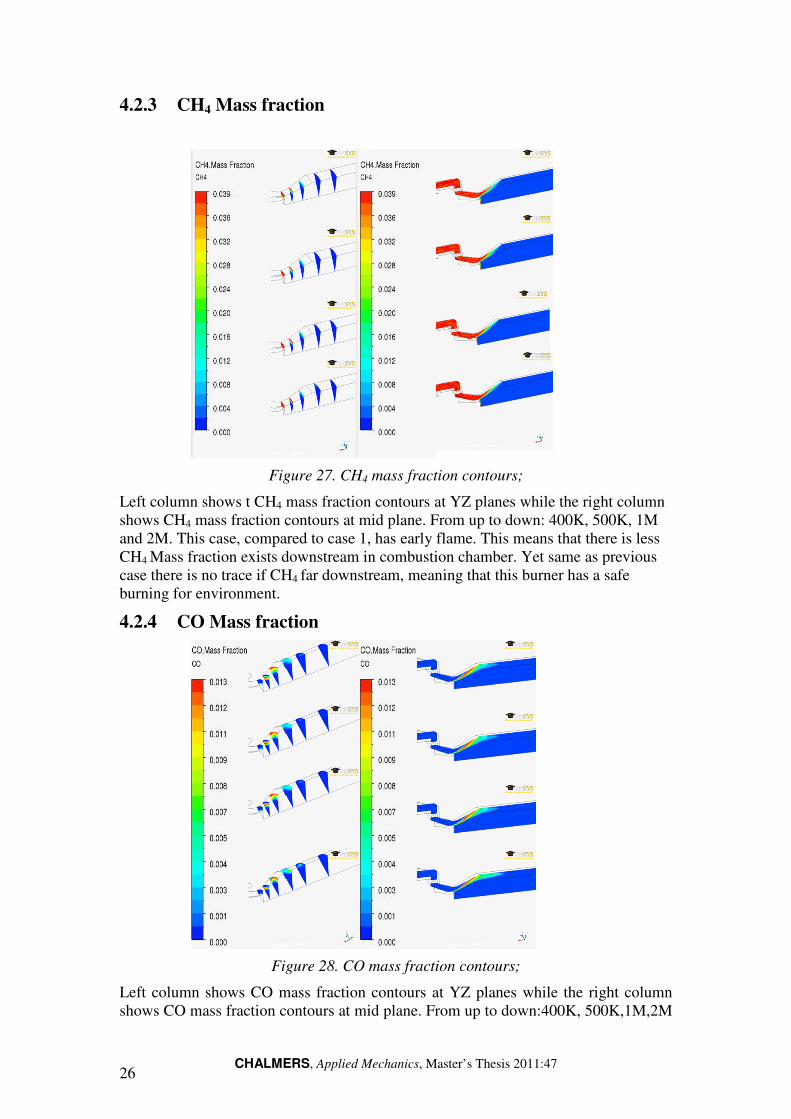
4.2.3 CH4 Mass fraction
Figure
Left column shows t CH4 mass fraction contours at YZ planes while the right column
shows CH4 mass fraction contours at mid plane. From up to down: 400K, 500K, 1M
and 2M. This case, compared to case 1, has early flame. This means that there is less
CH4 Mass fraction exists downstream in combustion chamber. Yet same as previous
case there is no trace if CH
burning for environment.
4.2.4 CO Mass fraction
Figure
Left column shows CO mass fraction contours at YZ planes while the right column
shows CO mass fraction contours at mid plane. F
CHALMERS, Applied Mechanics, Master’s Thesis 2011:47
Mass fraction
Figure 27. CH4 mass fraction contours;
mass fraction contours at YZ planes while the right column
mass fraction contours at mid plane. From up to down: 400K, 500K, 1M
. This case, compared to case 1, has early flame. This means that there is less
Mass fraction exists downstream in combustion chamber. Yet same as previous
ce if CH4 far downstream, meaning that this burner has a safe
CO Mass fraction
Figure 28. CO mass fraction contours;
Left column shows CO mass fraction contours at YZ planes while the right column
contours at mid plane. From up to down:400K, 500K,1M,
mass fraction contours at YZ planes while the right column
mass fraction contours at mid plane. From up to down: 400K, 500K, 1M
. This case, compared to case 1, has early flame. This means that there is less
Mass fraction exists downstream in combustion chamber. Yet same as previous
far downstream, meaning that this burner has a safe
Left column shows CO mass fraction contours at YZ planes while the right column
rom up to down:400K, 500K,1M,2M
Page 37
CHALMERS, Applied Mechanics, Master’s Thesis 2011:47 27
Flame shape can be predicted by looking at CO mass fraction. One can see that the
pattern for 2M case is bit different with other cases. That can be due the numerical
fluctuation in answer or numerical error.
4.2.5 Profile study
In this section we will study area average values of properties on YZ1, YZ2, YZ3 and
YZ 5.
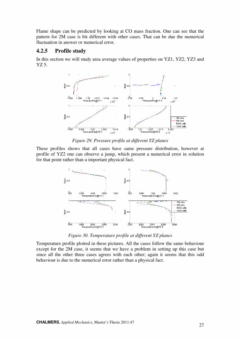
Figure 29. Pressure profile at different YZ planes
These profiles shows that all cases have same pressure distribution, however at
profile of YZ2 one can observe a jump, which present a numerical error in solution
for that point rather than a important physical fact.
Figure 30. Temperature profile at different YZ planes
Temperature profile plotted in these pictures. All the cases follow the same behaviour
except for the 2M case, it seems that we have a problem in setting up this case but
since all the other three cases agrees with each other; again it seems that this odd
behaviour is due to the numerical error rather than a physical fact.
Page 38
CHALMERS, Applied Mechanics, Master’s Thesis 2011:47 28
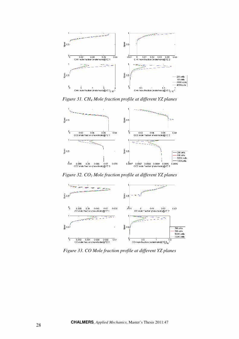
Figure 31. CH4 Mole fraction profile at different YZ planes
Figure 32. CO2 Mole fraction profile at different YZ planes
Figure 33. CO Mole fraction profile at different YZ planes
Page 39
CHALMERS, Applied Mechanics
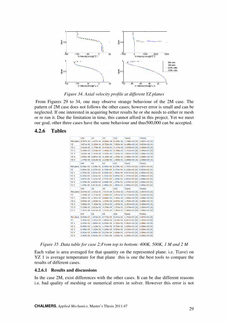
Figure 34. Axial velocity profile at different YZ planes
From Figures 29 to 34, one may observe strange behaviour of the 2M case
pattern of 2M case does not follows the other cases
neglected. If one interested in acquiring
or re run it. Due the limitation in time, this cannot afford in this project. Yet we meet
our goal, other three cases have the sam
4.2.6 Tables
Figure 35 .Data table for case 2
Each value is area averaged for that quantity on the represented plane. i.e. T(ave) on
YZ 1 is average temperature for
results of different cases.
4.2.6.1 Results and discussion
In the case 2M, exist differences with the other cases. It can be due different reasons
i.e. bad quality of meshing or numerical errors in solver. How
Mechanics, Master’s Thesis 2011:47
34. Axial velocity profile at different YZ planes
29 to 34, one may observe strange behaviour of the 2M case
pattern of 2M case does not follows the other cases; however error is small and can be
f one interested in acquiring better results he or she needs to either re mesh
or re run it. Due the limitation in time, this cannot afford in this project. Yet we meet
r goal, other three cases have the same behaviour and thus500,000 can be accepted.
35 .Data table for case 2;From top to bottom: 400K, 500K, 1 M and 2 M
Each value is area averaged for that quantity on the represented plane. i.e. T(ave) on
YZ 1 is average temperature for that plane this is one the best tools to compare the
discussions
In the case 2M, exist differences with the other cases. It can be due different reasons
i.e. bad quality of meshing or numerical errors in solver. However this error is not
29
29 to 34, one may observe strange behaviour of the 2M case. The
error is small and can be
needs to either re mesh
or re run it. Due the limitation in time, this cannot afford in this project. Yet we meet
e behaviour and thus500,000 can be accepted.
From top to bottom: 400K, 500K, 1 M and 2 M
Each value is area averaged for that quantity on the represented plane. i.e. T(ave) on
that plane this is one the best tools to compare the
In the case 2M, exist differences with the other cases. It can be due different reasons
ever this error is not
Page 40
CHALMERS, Applied Mechanics, Master’s Thesis 2011:47 30
critical since it is a case study and it seems that the 500K case agrees with the results
we excepted.
Page 41
CHALMERS, Applied Mechanics, Master’s Thesis 2011:47 31
5 Turbulence and heat transfer model study
In the previous two major cases, we have done grid study on a generic gas turbine
combustor. From the results, we choose 500,000 cells case, which presents both
accuracy and numerical speed.
In the following case we will use other variations in the turbulence models. Heat
transfer is also including for some of the cases in the study.
General boundary conditions and working condition are mentioned in section 3.3, but
for each of following cases, just one of settings was changed. New cases are:
• Case a: Turbulence model k-ε EARSM
• Case b: Turbulence model k-ε RNG
• Case c: Including conduction and convection with ambient using thin wall
interface , free stream temperature of 600K
• Case d: Turbulence model: k-ω SST, combustion model: finite rate and eddy
dissipation
• Case e: Top wall has heat transfer coefficient of 54.459 x
yG)
Used heat transfer coefficient was calculated. Calculations are shown in the appendix,
section 7.2.
5.1 Software limitation for thin wall interface
In order to model conduction and convection, we use thin wall interface, a new
feature in ANSYS CFX 12.1. The limitation of software implies that this interface
should be within the computational domain but not as a boundary. Thus we have to
add an additional domain to previously meshed domain which is illustrated in Figure
36. All the boundaries of this additional domain are opening with atmospheric
pressure.
Figure 36. Additional domain
5.2 Case three
In this case different features of different models will be discussed. As mentioned in
section 5, different models will be used. Aim of this case is to compare results based
on different turbulence models or heat transfer models.
Page 42
CHALMERS, Applied Mechanics, Master’s Thesis 2011:47 32
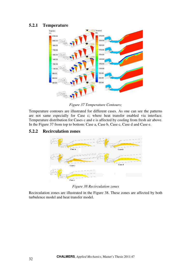
5.2.1 Temperature
Figure 37 Temperature Contours;
Temperature contours are illustrated for different cases. As one can see the patterns
are not same especially for Case c; where heat transfer enabled via interface.
Temperature distribution for Cases c and e is affected by cooling from fresh air above.
In the Figure 37 from top to bottom: Case a, Case b, Case c, Case d and Case e.
5.2.2 Recirculation zones
Figure 38 Recirculation zones
Recirculation zones are illustrated in the Figure 38. These zones are affected by both
turbulence model and heat transfer model.
Page 43
CHALMERS, Applied Mechanics, Master’s Thesis 2011:47 33
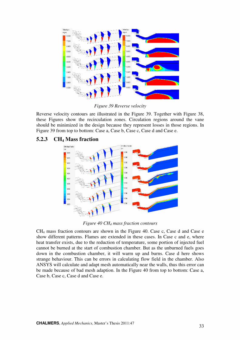
Figure 39 Reverse velocity
Reverse velocity contours are illustrated in the Figure 39. Together with Figure 38,
these Figures show the recirculation zones. Circulation regions around the vane
should be minimized in the design because they represent losses in those regions. In
Figure 39 from top to bottom: Case a, Case b, Case c, Case d and Case e.
5.2.3 CH4 Mass fraction
Figure 40 CH4 mass fraction contours
CH4 mass fraction contours are shown in the Figure 40. Case c, Case d and Case e
show different patterns. Flames are extended in these cases. In Case c and e, where
heat transfer exists, due to the reduction of temperature, some portion of injected fuel
cannot be burned at the start of combustion chamber. But as the unburned fuels goes
down in the combustion chamber, it will warm up and burns. Case d here shows
strange behaviour. This can be errors in calculating flow field in the chamber. Also
ANSYS will calculate and adapt mesh automatically near the walls, thus this error can
be made because of bad mesh adaption. In the Figure 40 from top to bottom: Case a,
Case b, Case c, Case d and Case e.
Page 44
CHALMERS, Applied Mechanics, Master’s Thesis 2011:47 34
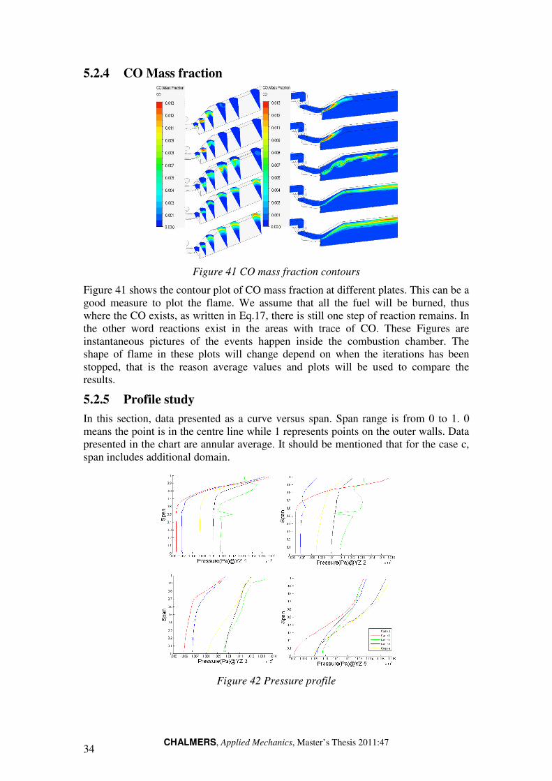
5.2.4 CO Mass fraction
Figure 41 CO mass fraction contours
Figure 41 shows the contour plot of CO mass fraction at different plates. This can be a
good measure to plot the flame. We assume that all the fuel will be burned, thus
where the CO exists, as written in Eq.17, there is still one step of reaction remains. In
the other word reactions exist in the areas with trace of CO. These Figures are
instantaneous pictures of the events happen inside the combustion chamber. The
shape of flame in these plots will change depend on when the iterations has been
stopped, that is the reason average values and plots will be used to compare the
results.
5.2.5 Profile study
In this section, data presented as a curve versus span. Span range is from 0 to 1. 0
means the point is in the centre line while 1 represents points on the outer walls. Data
presented in the chart are annular average. It should be mentioned that for the case c,
span includes additional domain.
Figure 42 Pressure profile
Page 45
CHALMERS, Applied Mechanics, Master’s Thesis 2011:47 35
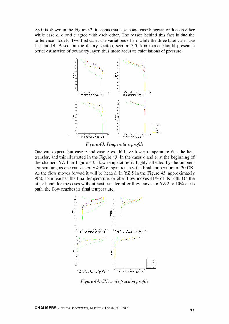
As it is shown in the Figure 42, it seems that case a and case b agrees with each other
while case c, d and e agree with each other. The reason behind this fact is due the
turbulence models. Two first cases use variations of k-ε while the three later cases use
k-ω model. Based on the theory section, section 3.5, k-ω model should present a
better estimation of boundary layer, thus more accurate calculations of pressure.
`
Figure 43. Temperature profile
One can expect that case c and case e would have lower temperature due the heat
transfer, and this illustrated in the Figure 43. In the cases c and e, at the beginning of
the chamer, YZ 1 in Figure 43, flow temperature is highly affected by the ambient
temperature, as one can see only 40% of span reaches the final temperature of 2000K.
As the flow moves forwad it will be heated. In YZ 5 in the Figure 43, approximately
90% span reaches the final temperature, or after flow moves 41% of its path. On the
other hand, for the cases without heat transfer, after flow moves to YZ 2 or 10% of its
path, the flow reaches its final temperature.
Figure 44. CH4 mole fraction profile
Page 46
CHALMERS, Applied Mechanics, Master’s Thesis 2011:47 36
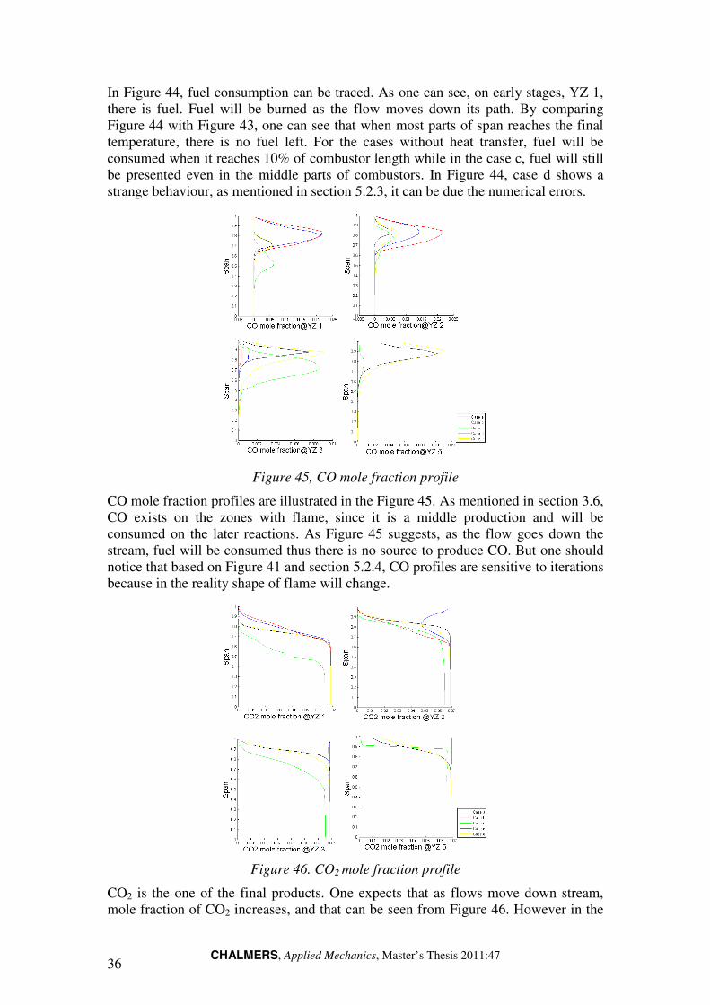
In Figure 44, fuel consumption can be traced. As one can see, on early stages, YZ 1,
there is fuel. Fuel will be burned as the flow moves down its path. By comparing
Figure 44 with Figure 43, one can see that when most parts of span reaches the final
temperature, there is no fuel left. For the cases without heat transfer, fuel will be
consumed when it reaches 10% of combustor length while in the case c, fuel will still
be presented even in the middle parts of combustors. In Figure 44, case d shows a
strange behaviour, as mentioned in section 5.2.3, it can be due the numerical errors.
Figure 45, CO mole fraction profile
CO mole fraction profiles are illustrated in the Figure 45. As mentioned in section 3.6,
CO exists on the zones with flame, since it is a middle production and will be
consumed on the later reactions. As Figure 45 suggests, as the flow goes down the
stream, fuel will be consumed thus there is no source to produce CO. But one should
notice that based on Figure 41 and section 5.2.4, CO profiles are sensitive to iterations
because in the reality shape of flame will change.
Figure 46. CO2 mole fraction profile
CO2 is the one of the final products. One expects that as flows move down stream,
mole fraction of CO2 increases, and that can be seen from Figure 46. However in the
Page 47
CHALMERS, Applied Mechanics, Master’s Thesis 2011:47 37
case c and case e, production rate of CO2 is less than other cases. As mentioned before
the reason behind this fact is due the cooling effects of environment, reaction rate of
combustion will drop, thus less CO2 will be produced compared with the cases
without heat transfer.
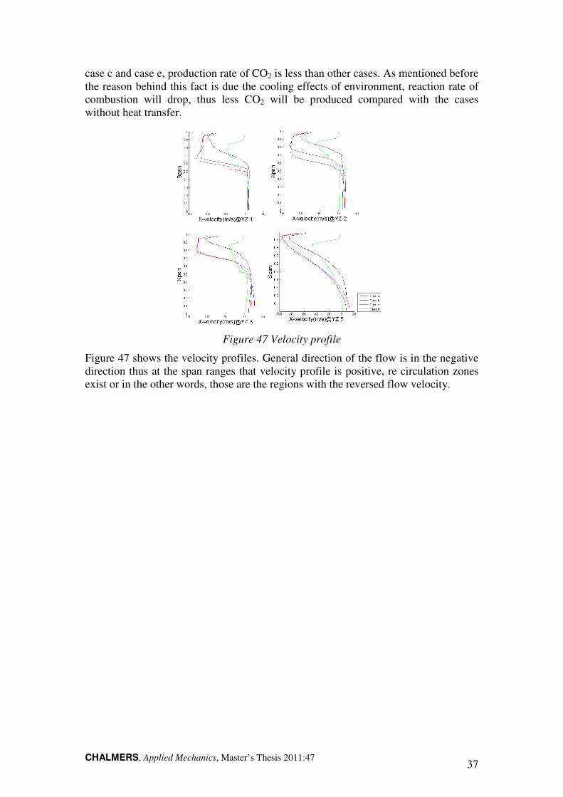
Figure 47 Velocity profile
Figure 47 shows the velocity profiles. General direction of the flow is in the negative
direction thus at the span ranges that velocity profile is positive, re circulation zones
exist or in the other words, those are the regions with the reversed flow velocity.
Page 48
CHALMERS, Applied Mechanics, Master’s Thesis 2011:47 38
5.2.6 Table
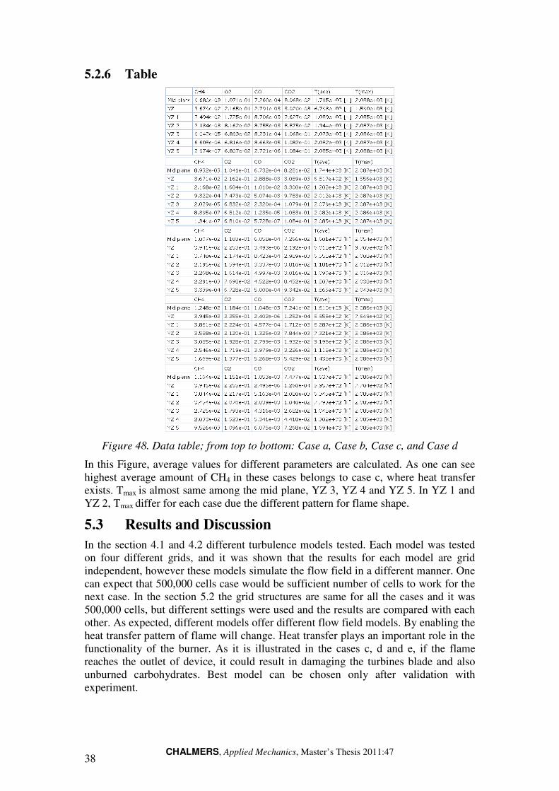
Figure 48. Data table; from top to bottom: Case a, Case b, Case c, and Case d
In this Figure, average values for different parameters are calculated. As one can see
highest average amount of CH4 in these cases belongs to case c, where heat transfer
exists. Tmax is almost same among the mid plane, YZ 3, YZ 4 and YZ 5. In YZ 1 and
YZ 2, Tmax differ for each case due the different pattern for flame shape.
5.3 Results and Discussion
In the section 4.1 and 4.2 different turbulence models tested. Each model was tested
on four different grids, and it was shown that the results for each model are grid
independent, however these models simulate the flow field in a different manner. One
can expect that 500,000 cells case would be sufficient number of cells to work for the
next case. In the section 5.2 the grid structures are same for all the cases and it was
500,000 cells, but different settings were used and the results are compared with each
other. As expected, different models offer different flow field models. By enabling the
heat transfer pattern of flame will change. Heat transfer plays an important role in the
functionality of the burner. As it is illustrated in the cases c, d and e, if the flame
reaches the outlet of device, it could result in damaging the turbines blade and also
unburned carbohydrates. Best model can be chosen only after validation with
experiment.
Page 49
CHALMERS, Applied Mechanics, Master’s Thesis 2011:47 39
6 Conclusion
It should be mentioned in the pressure plots and pressure profile of cases, pressure
distribution may vary with number of iteration and that is the reason the plots and
charts may vary. The variation of the pressure fall into acceptable error range for
numerical error, thus the results were accepted.
The conclusion from the grid-study is that the mesh-size that is used for the 500K case
is enough, or in other words the results are grid-independent. These conclusions are
based on steady-state simulations and were not tested on transient simulations due to
limitations of time in the project. This is also important to check in the future work.
The 500k mesh size would imply that the number of cells for a full 360o model would
be approximately 16M cells.
By consider all the three cases; the recommendation is to use the k-ω SST model with
heat transfer for the steady-state simulations. Because this model showed stable
convergence and also it predicts flow field better than the other cases.
6.1 Future works
The suggestion for future work is to test more models. Also, the simulations done in
this work uses CH4 as fuel, while there are varieties of fuels available to use.
Suggestion for future work:
• Test the open source software OpenFOAM
• Test different fuels
• Modelling the generic gas turbine combustor with different inlets for fuel and
air and use pre heated air.
• Grid study for transient simulations
Page 50
CHALMERS, Applied Mechanics, Master’s Thesis 2011:47 40
Page 51
CHALMERS, Applied Mechanics, Master’s Thesis 2011:47 41
7 References
1- http://en.wikipedia.org/wiki/Gas_turbine
2- H. K. Versteeg, W. Malalasekera, An Introduction to Computational Fluid
Dynamic. Second edition. London: Prentice Hall
3- Menter, F. R., Kuntz, M., Langtry, R., Ten Years of Industrial Experience with
the SST Turbulence Model, Turbulence, Heat and Mass Transfer 4, Begell
House, 2003, pp. 625-632
4- Charles K. Westbrook, Frederick L. Dryer, Chemical kinetics and modelling
of combustion processes, Journal of Symposium (International) on
combustion, Volume 18, Issue 1, pp. 749-767
5- http://iceberg2.shef.ac.uk/docs/cfx-pdf/reference/Combustion.pdf
6- ANSYS CFX®
v12.1 User Manual
7- J.C. Kok, Resolving the dependence on free stream values for k-omega
turbulence model, Nationaal Lucht- en Ruimtevaartlaboratorium, 1999
8- R. J. A. Howarda, D. Toporovb, The eddy dissipation combustion model
developed for large eddy simulation.
7.1 Picture references
p1- http://gcaptain.com/ship-engines-hood-monster-engines?9883
p2- http://www.bloodhoundssc.com/car/jet_propulsion.cfm
p3- http://www.citizendia.org/Turboshaft
Page 52
CHALMERS, Applied Mechanics, Master’s Thesis 2011:47 42
Page 53
CHALMERS, Applied Mechanics
8 Appendix
8.1 Pictures
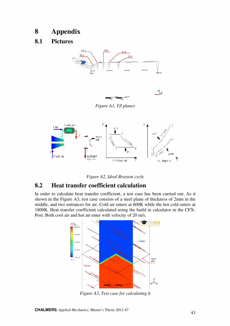
8.2 Heat transfer coefficient calculation
In order to calculate heat transfer coefficient, a test
shown in the Figure A3, test case consists of a steel plane of thickness of 2mm in the
middle, and two entrances for air. Cold air enters at 600K while the hot cold enters at
1800K. Heat transfer coefficient calcula
Post. Both cool air and hot air enter with velocity of 20 m/s.
Figure
Mechanics, Master’s Thesis 2011:47
Figure A1, YZ planes
Figure A2, Ideal Brayton cycle
Heat transfer coefficient calculation
In order to calculate heat transfer coefficient, a test case has been carried out.
, test case consists of a steel plane of thickness of 2mm in the
and two entrances for air. Cold air enters at 600K while the hot cold enters at
1800K. Heat transfer coefficient calculated using the build in calculator in the CFX
Both cool air and hot air enter with velocity of 20 m/s.
Figure A3, Test case for calculating h
43
case has been carried out. As it
, test case consists of a steel plane of thickness of 2mm in the
and two entrances for air. Cold air enters at 600K while the hot cold enters at
ted using the build in calculator in the CFX-


![CFD Modelling for Smoke Movementfe.hkie.org.hk/Upload/Doc/4c0725e5-5732-4355-9885... · CFD modelling examples 27 . Temperature Visibility [CO] 28 Key Parameters from CFD simulation](https://static.documents.pub/doc/80x56/5e903441bf32a85bcb51aef9/cfd-modelling-for-smoke-cfd-modelling-examples-27-temperature-visibility-co.jpg)


