22.38 PROBABILITY AND ITS APPLICATIONS TORELIABILITY, QUALITY CONTROL AND RISK ASSESSMENT

Fall 2005, Lecture 2

RISK-INFORMED OPERATIONALDECISION MANAGEMENT (RIODM):RELIABILITY AND AVAILABILITY

Michael W. GolayProfessor of Nuclear Engineering

Massachusetts Institute of Technology

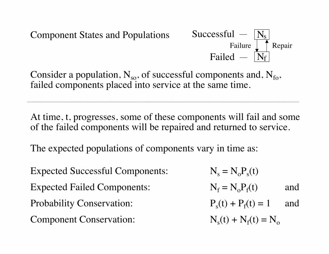
Component States and Populations Successful Failure

Ns

Nf

Repair Failed

Consider a population, Nso, of successful components and, Nfo, failed components placed into service at the same time.

At time, t, progresses, some of these components will fail and someof the failed components will be repaired and returned to service.

The expected populations of components vary in time as:

Expected Successful Components: Ns = NoPs(t) Expected Failed Components: Nf = NoPf(t) and Probability Conservation: Ps(t) + Pf(t) = 1 and Component Conservation: Ns(t) + Nf(t) = No

COMPONENT FAILURE PROBABILITYComponent (Conditional) Failure Rate, λ(t),

1Ps t( )

dPs t( )dt

=1

Ns t( )dNs t( )dt

= −λ t( )

wherePs(t) = probability that an individual component will be

successful at time, t;Ns(t) = expected number of components surviving at time, t (note

that Ns(t=0) = Nso);λ(t) = time-dependent (conditional) failure rate function.

Mean-Time-To-Failure (MTTF) = 1/λ = τf,

for λ = constant.

COMPONENT REPAIR PROBABILITYComponent Repair Coefficient, µ(t),

1Pf t( )

dPf t( )dt

=1

Nf t( )dNf t( )dt

= −µ t( )

wherePf(t) = probability that an individual component will be failed at

time, t;Nf(t) = expected number of components failed at time, t (note that

Nf(t=0) = Nfo);µ(t) = time-dependent (conditional) repair rate function.

Mean-Time-To-Repair (MTTR) = 1/µ = τR,

for µ = constant.

Combined Repair and FailuredNsdt

= −λNs t( ) + µNf t( )

dNfdt

= λNs t( ) − µNf t( )

can express as matrix equationdN dt

= MN ,where

N =Ns t( )

Nf t( )

, and M =

−λ µ

λ −µ

.

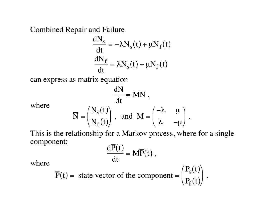
This is the relationship for a Markov process, where for a singlecomponent:

dP t( )dt

= MP t( ) ,where

P t( ) = state vector of the component =Ps t( )

Pf t( )

.

For initial condition Ps(t=0) = 1 and Pf(t=0) = 0,

Solution is:Ps t( ) =

µ

λ + µ+

λ

λ + µ

e− λ+µ( ) t

Pf t( ) =λ

λ + µ

1− e− λ+µ( )t[ ] .

Asymptotic result: (i.e., as t ∅ ∞)

Ps∞ =µ

λ + µ

, Pf∞ =

λ

λ + µ

.

a

1

00 Time, t

Pf∞

Ps∞Ps

Pf

COMPONENT CYCLE: RUN-TO-FAILURE,REPAIR AND RETURN-TO-SERVICE

Consider that total mean cycle time is τcycle for:Component Statusa) Serviceb) Failurec) Waiting for repaird) Repaired to service

τcycle = τs + τR =1λ+1µ=µ + λ

λµ

Ps∞ =τs

τcycle=

µ

µ + λ

Pf∞ =τRτcycle

=λ

µ + λ

= τs (= MTTF)

= τR (= MTTR)

a

τR

τcycleτs

EFFECTS OF COMPONENTTESTING AND INSPECTION

• Verify That Component Is Operable• Reveal Failures That Can Be Repaired• Exercise Component and Maintain Operability• Maintain Skills of Testing Team

BENEFICIAL

• Removal From Service Can Result in Complete ComponentUnavailability

• Wear and Tear Due to Testing (Wear, Fatigue, Corrosion, …)• Introduction of New Defects (e.g., via Damage During Inspection,

Fuel Depletion)• Acceleration of Dependent Failures• Damage or Degradation of Component via Incorrect Restoration to

Service• Human Error Can Cause Wrong Component to Be Removed From

Service

HARMFUL

TIME DEPENDENCE OF STANDBYCOMPONENT UNAVAILABILITY,INCLUDING TEST AND REPAIR

aa

1.0

0Time, tt1 t 2

t1 = time of first test

TestTest

Effect of tests, dem-onstrating that somefailure modes havenot become activated

Effect of untested failure modes andnew defects

Meanrepair, t ,duration

ti = time of i-th test

f ,fraction

of testedcomponents

requiring repair

R

Q1 Q2

Test, t ,duration

t

R

POST-TEST UNAVAILABILITY

• Failures Requiring Repairs, Caused by Tests

• Defects Introduced by Tests, Resulting in Later Failures

• Incorrect Component (and Supporting System)Disengagement, Re-Engagement

• Incorrect Component Having Been Tested

CAUSED BY

MEAN AVAILABILITY, <Q>, UNDERDIFFERENT COMBINATIONS OF TESTINGAND REPAIR: CASES TO BE CONSIDERED

(λ = CONSTANT)

1. Asymptotic Component Unavailability as Function of µ, λ2. Mean Component Unavailability During Standby Interval3. Cycle Mean Unavailability Due to

• Defects randomly introduced during standby,• Unavailability due to testing and repairs

4. Cycle Mean Unavailability Due to• Pre-existing defects,• Defects introduced during standby, and• Unavailability due to testing and repairs

5. Standby Interval That Minimizes <Q>

CASES

CASE 1. ASYMPTOTIC AVAILABILITY WHENFAILURES ARE MONITORED AND REPAIRED

Asymptotic Availability : A∞ = Ps∞ =µ

µ + λ

Note that MTTR (TD = repair-related down-time)=1µ= TD

⇒ A =1

1+ λTD and Q = 1− A =

λTD1+ λTD

also, Q ≈ λTD

a

1

0 0 Time, tPf∞

Ps∞Ps

Pf

CASE 2. MEAN UNAVAILABILITYDURING STANDBY PERIOD, ts

During Standby : Q t( ) = Pf t( ) = 1 − e−λts ≈ 1− 1− λts( )Q t( ) ≈ λts

a

Time

<Q>

Pf

ts

€

Q =tDtc

=Q ′ t ( )d ′ t 0

ts∫ts

=λ ′ t ( )d ′ t 0

ts∫ts

= λts2

2ts

Q = λts2

tc = cycle time

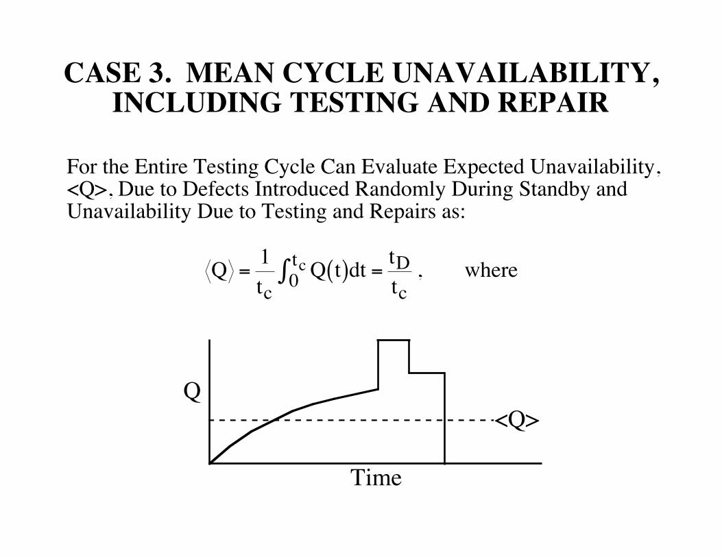
CASE 3. MEAN CYCLE UNAVAILABILITY,INCLUDING TESTING AND REPAIR

For the Entire Testing Cycle Can Evaluate Expected Unavailability,<Q>, Due to Defects Introduced Randomly During Standby andUnavailability Due to Testing and Repairs as:

€

Q =1tc

Q t( )dt =tDtc, where0

tc∫

a

Time

<Q>Q

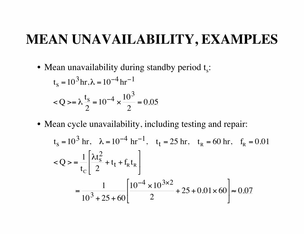
CASE 3. MEAN CYCLE UNAVAILABILITY(continued)

DOWNTIME: tD = tDs + tDt + tDR

During Standby: tDs =λts2

2During Testing: tDt = ttDuring Repair: tDR = fRtRfR = repair frequency, the fraction of tests for which a repair is

requiredCYCLE TIME: tc = ts + tt + tR

cycle standby testing repair

AVERAGE UNAVAILABILITY:

€

Q =tDtc

=1tc∗λts2

2+ tt + fRtR

ts + tt + tR( )

CASE 4. MEAN CYCLE UNAVAILABILITY,INCLUDING PRE-EXISTING

UNAVAILABILITY, Qo

Evaluate Expected System Unavailability, <Q>, Due to• Pre-Existing Defects• Defects Introduced Randomly During Standby and• Unavailability Due to Testing and Repairs as:

a

Time

<Q>Q

Qo

CASE 4. MEAN CYCLE UNAVAILABILITY,INCLUDING PRE-EXISTING UNAVAILABILITY,

Qo (continued)DOWNTIME: tD = tDs + tDt + tDR

During Standby: tDs = Qots +λ

2ts2 1−Qo( )

During Testing: tDt = ttDuring Repair: tDR = fRtR

Qo = expected unavailability due to pre-existing defects (i.e.,those not interrogated during testing)

CYCLE TIME: tc = ts + tt + tRcycle standby testing repair

AVERAGE UNAVAILABILITY:

Q =tDtc

=1tc

Qots + 1−Qo( )λ

2ts2

+ tt + fRtR

For Entire Cycle: tD = Qots + 1−Qo( )λ

2ts2 + t t + fRtR

COMBINED CASE OF EFFECT UPON STANDBYSYSTEM FAILURE OF PRE-EXISTING FAULT

AND RANDOMLY INTRODUCED FAULT

a

I R I = Pre-existing fault event

R = Random fault event

F = I+R = Component fault

P F( ) = P I + R( ) = P I( ) + P R( ) − P I( ) ⋅P R( )

P F( ) = Qo +λts2−Qo ⋅

λts2

P F( ) = Qo + 1−Qo( )λts2

CASE 5. STANDBY INTERVAL THATMINIMIZES <Q>

For a Good System: t t + fRtR << ts

€

Qo <<1

€

⇒ Q ≈1tcQots +

λ2ts2 + tt + fRtR

€

The value of ts which minimizes Q , ts*, is obtained from ∂ Q∂ts

= 0 as

ts* =

2 t t + fRtR( )λ

1/ 2

= 2τf t t + fRtR( )[ ]1/ 2

τf = random defects contribution(tt + fRtR) = testing and repair contribution

UNAVAILABILITY

• Failure density• Cumulative Density Function (CDF):• Unavailability

probability that system is down at time t,

fT (t) = λe−λt t ≥ 0

€

Q(t) :FT(t) = P(T ≤ t) = fT (t)dt

0

t

∫

€

Q(t) = FT(t) = fT(t)dt =1− e−λt ≈ 1− (1−λt)0t∫

Q(t) ≈ λt

MEAN UNAVAILABILITY DURINGSTANDBY PERIOD, ts

€

<Q >=1ts

Q(t)dt ≈ λtdt = λts2

2ts0ts∫0

ts∫

<Q >≈ λts2

MEAN CYCLE UNAVAILABILITY,INCLUDING TESTING AND REPAIR

Q(t)

<Q>

Timets

tt

tR

tC

€

Q(t) =

λt1fR

(0 ≤ t ≤ ts )(ts < t ≤ ts + tt )(ts + tt < t ≤ t C )

€

<Q > =1tC× Q(t)dt0

tC∫

=1tC× λtdt+ dtts

ts+t t∫ +0ts∫ fRdtts+t t

tC∫[ ]=1tC×λ2ts2 + tt + fRtR

MEAN CYCLE UNAVAILABILITY INCLUDINGPRE-EXISTING UNAVAILABILITY, Q0

Q(t)

<Q>

Timets

tt

tR

tC

Q0

€

Q(t) =

Q0 + (1−Q0)λt1fR

(0 ≤ t ≤ ts )(ts < t ≤ ts + tt )(ts + tt < t ≤ t C )

€

<Q > =1tC× Q(t)dt0

tC∫

=1tC× Q0 + (1−Q0)λtdt+ dtts

ts+t t∫ +0ts∫ fRdtts+t t

tC∫[ ]=1tC× Q0ts + (1−Q0)

λ2ts2

+ tt + fRtR

STANDBY INTERVAL, ts*, THAT

MINIMIZES <Q>

•

• For a good system

€

<Q >=1tC× Q0ts + (1−Q0)

λ2ts2

+ tt + fRtR

€

⇒ <Q > ≈1ts× Q0t+

λ2ts2

+ tt + fRtR

∂ <Q >∂ts

(ts*) = 0

∂ <Q >∂ts

(ts*) =λ2− (tt + fRtR )×

1ts*2 = 0

⇒ ts* =2(tt + fRtR )

λ

1/2

€

tt + fRtR << tsQ0 <<1

⇒tC = ts + tt + tR ≈ ts

(1−Q0) ≈ 1

STANDBY INTERVAL, ts*, THAT

MINIMIZES <Q> (continued)

<Q>

tC

1

ts*

€

ts* =2(tt + fRtR )

λ

1/2= 2τf tt + fRtR( )[ ]1/2

tf = random defects contribution

(tt+fRtR) = testing and repair contribution

MEAN UNAVAILABILITY, EXAMPLES

• Mean unavailability during standby period ts:

• Mean cycle unavailability, including testing and repair:

€

ts =103hr,λ =10−4hr−1

<Q >= λts2

=10−4 ×103

2= 0.05

€

ts =103 hr, λ =10−4 hr−1, tt = 25 hr, tR = 60 hr, fR = 0.01

<Q > =1tC

λts2

2+ tt + fRtR

=1

103 + 25+ 6010−4 ×103×2

2+ 25+ 0.01× 60

≈ 0.07

MEAN UNAVAILABILITY, EXAMPLES(continued)

• Mean cycle unavailability including Q0:

• Optimum standby interval ts:

€

ts =103 hr, λ =10−4 hr−1, tt = 25 hr, tR = 60 hr, fR = 0.01, Q0 = 0.02

<Q > =1tCQ0ts + (1−Q0)

λts2

2+ tt + fRtR

=1

103 + 25+ 600.02×103 + (1− 0.02)10

−4 ×103×2

2+ 25+ 0.01× 60

≈ 0.087

€

ts* =2(tt + fRtR )

λ

1/2=2(25+ 0.01× 60)

10−4

1/2≈ 715.54 hr

EXAMINATION OF SEQUENCING OF TESTS

EXAMPLE OF TWO PARALLEL IDENTICAL COMPONENTS*

A) Successive Testing

B) Staggered Testing

* • Consider random failures during standby, time out-of-service during testing • Ignore time out-of-service during repairs, pre-existing defects.

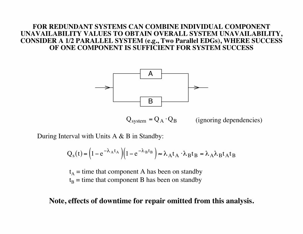
FOR REDUNDANT SYSTEMS CAN COMBINE INDIVIDUAL COMPONENTUNAVAILABILITY VALUES TO OBTAIN OVERALL SYSTEM UNAVAILABILITY,CONSIDER A 1/2 PARALLEL SYSTEM (e.g., Two Parallel EDGs), WHERE SUCCESS

OF ONE COMPONENT IS SUFFICIENT FOR SYSTEM SUCCESS

a

A

B

Qsystem = QA ⋅QB (ignoring dependencies)

During Interval with Units A & B in Standby:

Qs t( ) = 1− e−λA tA( ) 1− e−λBtB( ) ≈ λAtA ⋅λBtB = λAλBtAtBtA = time that component A has been on standbytB = time that component B has been on standby

Note, effects of downtime for repair omitted from this analysis.

Qs = fRB 1− e−λA tA( ) ≈ fRB ⋅λAtA

FOR REDUNDANT SYSTEMS CAN COMBINE INDIVIDUAL COMPONENTUNAVAILABILITY VALUES TO OBTAIN OVERALL SYSTEM UNAVAILABILITY,CONSIDER A 1/2 PARALLEL SYSTEM (e.g., Two Parallel EDGs), WHERE SUCCESS

OF ONE COMPONENT IS SUFFICIENT FOR SYSTEM SUCCESS (continued)

Qs = 1⋅ 1− e−λBt B( ) ≈ λBtBDuring Interval with Unit A in Testing:

Qs = 1− e−λA tA( ) ⋅1 ≈ λAtADuring Interval with Unit B in Testing:

Qs = fRA 1− e−λBt B( ) ≈ fRA ⋅λBtBDuring Interval with Unit A Possibly in Repair:

where fR A= repair frequency of Unit A

During Interval with Unit B Possibly in Repair:

where fR B= repair frequency of Unit B

ILLUSTRATION OF INDIVIDUAL COMPONENT (e.g., EDG) UNRELIABILITIESFOR A 1/2 PARALLEL SYSTEM GIVEN A STRATEGY OF TESTING EACH

COMPONENT AT SUCCESSIVE INTERVALS (e.g., TESTING BOTHCOMPONENTS DURING SAME OUTAGE)*

Component ATested First

Component BTested Second

Let λA = λB = λTesting Time Start

Component A Component Bτ1 = τ τ1′ = τ + tt

τ2 = 2τ + tt τ2′ = τ2 + tt - 2τ + 2tt

* Role of repair omitted from the analysis.

ILLUSTRATION OF INDIVIDUAL COMPONENT (e.g., EDG) UNRELIABILITYFOR A 1/2 PARALLEL SYSTEM GIVEN A STRATEGY OF TESTING EACH

COMPONENT AT EVENLY STAGGERED INTERVALS

Component ATested First

Component BTested Second

COMPARISON OF MAXIMUM AND AVERAGEVALUES OF Q, FIRST CYCLE OF TESTING

Successive Testing:

€

λ τ + tt( ) ≈ λτ

Staggered Testing:

€

λτ2

+ tt

≈ λ

τ2

Qmax

Successive Testing:

€

≈λτ3

Staggered Testing:

€

≈524λτ

<Q>cycle

HUMAN ERRORS ARETYPICALLY MOST IMPORTANT

Also, taking into account human errors committed during testsand repair and failure modes not tested previously.

Qo = unavailability due to defects existing at the start of thenext testing cycle

Qo = QU +QH , whereQU = unavailability due to failure modes not interrogated during

the tests performed, and those activated upon demandQH = λttt + λRtR, and λt = rate of introduction of defects due to human errors during

tests (e.g., system realignment errors), hr -1

λR = rate of introduction of defects due to human errors duringrepairs (e.g., incorrectly installed gaskets, tools or debrisleft within a component), hr -1

SUMMARY

• Testing and Inspections Contribute to Simultaneous Increasesand Decreases in System Availability

• These Contributions Can Be Balanced Optimally

• Staggered Testing Yield Lower Peak and Lower Mean SystemUnavailability vs. Successive Testing