1 2.3. Quantitative Properties of Finite Difference Schemes 2.3.1. Consistency, Convergence and Stability of F.D. schemes Reading: Tannehill et al. Sections 3.3.3 and 3.3.4. Three important properties of F.D. schemes: Consistency – An F.D. representation of a PDE is consistent if the difference between PDE and FDE, i.e., the truncation error, vanishes as the grid interval and time step size approach zero , i.e., when 0 lim(PDE FDE) 0 Δ→ − = . Comment: • Consistency deals with how well the FDE approximates the PDE. Stability – For a stable numerical scheme, the errors from any source will not grow unboundedly with time. Comments: • A concept that is applicable only to marching (time-integration) problems. • Generally we are much more concerned with stability than consistency. • Some hard work is often needed to establish analytically the stability of a scheme. Convergence – It means that the solution to a FDE approaches the true solution to the PDE as both grid interval and time step size are reduced.
Transcript
1
2.3. Quantitative Properties of Finite Difference Schemes
2.3.1. Consistency, Convergence and Stability of F.D. schemes Reading: Tannehill et al. Sections 3.3.3 and 3.3.4. Three important properties of F.D. schemes: Consistency – An F.D. representation of a PDE is consistent if the difference between PDE and FDE, i.e., the
truncation error, vanishes as the grid interval and time step size approach zero,
i.e., when 0
lim(PDE FDE) 0Δ→
− = .
Comment:
• Consistency deals with how well the FDE approximates the PDE. Stability – For a stable numerical scheme, the errors from any source will not grow unboundedly with time. Comments:
• A concept that is applicable only to marching (time-integration) problems. • Generally we are much more concerned with stability than consistency. • Some hard work is often needed to establish analytically the stability of a scheme.
Convergence – It means that the solution to a FDE approaches the true solution to the PDE as both grid interval
and time step size are reduced.
2
Lax's Equivalence Theorem
For a well-posed, linear initial value problem, the necessary and sufficient condition for convergence is that the FDE is stable and consistent. The theorem has been proved for initial value problems governed by linear PDE's (Richtmyer and Morton 1967).
We will discuss the three concepts one by one.
2.3.2. Consistency Consistency means PDE FDE 0− → when Δx 0 and Δt 0. Clearly consistency is the necessary condition for convergence. Example: Consider a 1-D diffusion equation:
2
2 ( 0 and constant)u uK Kt x
∂ ∂= >
∂ ∂
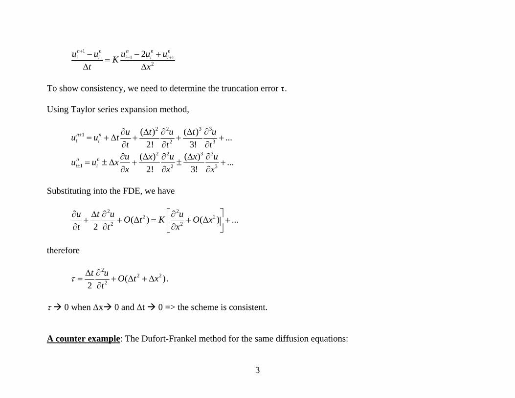
We use the forward-in-time and centered-in-space (FTCS) scheme:
3
11 1
2
2n n n n ni i i i iu u u u uK
t x
+− +− − +
=Δ Δ
To show consistency, we need to determine the truncation error τ. Using Taylor series expansion method,
2 2 3 31
2 3
( ) ( ) ...2! 3!
n ni i
u t u t uu u tt t t
+ ∂ Δ ∂ Δ ∂= + Δ + + +
∂ ∂ ∂
2 2 3 3
1 2 3
( ) ( ) ...2! 3!
n ni i
u x u x uu u xx x x±
∂ Δ ∂ Δ ∂= ± Δ + ± +
∂ ∂ ∂
Substituting into the FDE, we have
2 22 2
2 2( ) ( ) ...2
u t u uO t K O xt t x
⎡ ⎤∂ Δ ∂ ∂+ + Δ = + Δ +⎢ ⎥∂ ∂ ∂⎣ ⎦
therefore
22 2
2 ( )2t u O t x
tτ Δ ∂
= + Δ + Δ∂
.
τ 0 when Δx 0 and Δt 0 => the scheme is consistent.
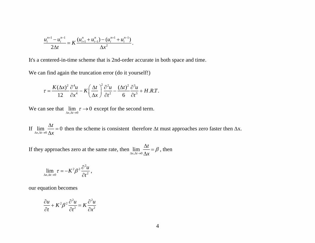
A counter example: The Dufort-Frankel method for the same diffusion equations:
4
1 1 1 1
1 12
( ) ( )2
n n n n n ni i i i i iu u u u u uK
t x
+ − + −+ −− + − +
=Δ Δ
.
It's a centered-in-time scheme that is 2nd-order accurate in both space and time. We can find again the truncation error (do it yourself!)
22 4 2 2 3
4 2 3
( ) ( ) . . .12 6
K x u t u t uK H R Tx x t t
τ Δ ∂ Δ ∂ Δ ∂⎛ ⎞= − − +⎜ ⎟∂ Δ ∂ ∂⎝ ⎠
We can see that
, 0lim 0x t
τΔ Δ →
→ except for the second term.
If , 0lim 0x t
txΔ Δ →
Δ=
Δ then the scheme is consistent therefore Δt must approaches zero faster then Δx.
If they approaches zero at the same rate, then, 0limx t
tx
βΔ Δ →
Δ=
Δ, then
2
2 22, 0
limx t
uKt
τ βΔ Δ →
∂= −
∂,
our equation becomes
2 22 2
2 2
u u uK Kt t x
β∂ ∂ ∂+ =
∂ ∂ ∂
5
Thus, we are solving the wrong equation. In fact this equation is hyperbolic instead of parabolic.
Note that if ~ 1tx
ΔΔ
you might see spurious waves in your solution, due to the hyperbolic nature of the "new" PDE.
2.3.3. Convergence General Discussion Definition is given earlier. Symbolically, it is
, 0lim ( , )n
ix tu u x t
Δ Δ →= .
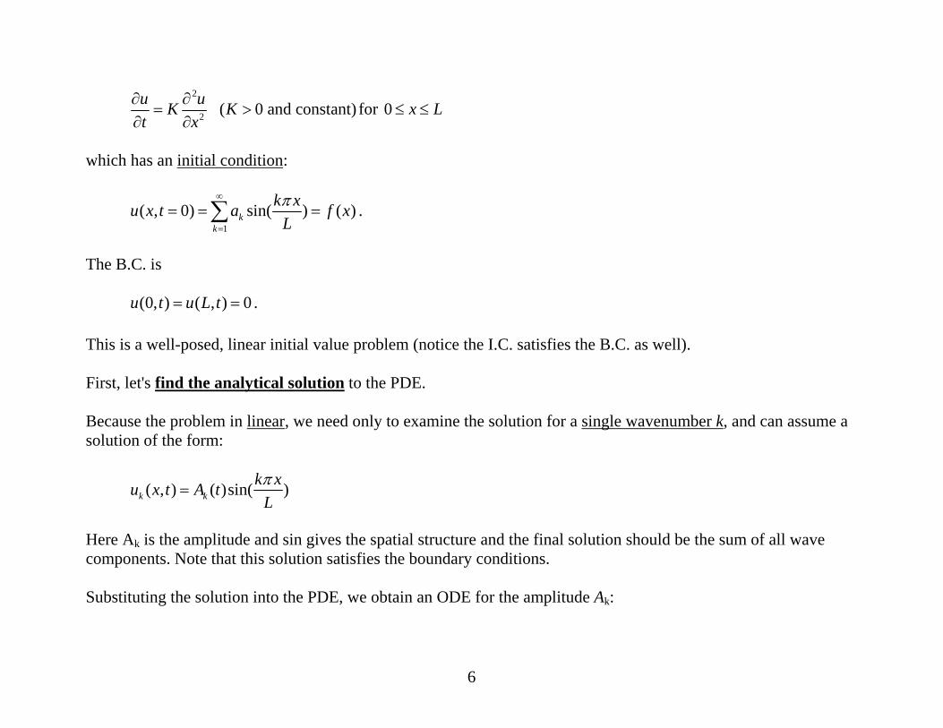
Convergence is generally hard to prove, especially for nonlinear problems. The Lax's Theorem we presented earlier is very helpful in understanding the convergence for linear systems, and is often extended to nonlinear systems. We will also discuss numerical convergence and methods for measuring solution accuracy later. We will first show a convergence proof for a diffusion problem. Certain concept introduced will be useful later. Convergence proof for a 1-D diffusion problem Consider
6
2
2 ( 0 and constant)u uK Kt x
∂ ∂= >
∂ ∂for 0 x L≤ ≤
which has an initial condition:
1
( , 0) sin( ) ( )kk
k xu x t a f xLπ∞
=
= = =∑ .
The B.C. is (0, ) ( , ) 0u t u L t= = . This is a well-posed, linear initial value problem (notice the I.C. satisfies the B.C. as well). First, let's find the analytical solution to the PDE. Because the problem in linear, we need only to examine the solution for a single wavenumber k, and can assume a solution of the form:
( , ) ( )sin( )k kk xu x t A t
Lπ
=
Here Ak is the amplitude and sin gives the spatial structure and the final solution should be the sum of all wave components. Note that this solution satisfies the boundary conditions. Substituting the solution into the PDE, we obtain an ODE for the amplitude Ak:
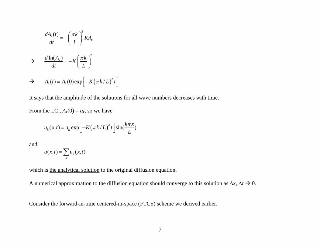
7
2( )kk
dA t k KAdt L
π⎛ ⎞= −⎜ ⎟⎝ ⎠
2ln( )kd A kK
dt Lπ⎛ ⎞= − ⎜ ⎟
⎝ ⎠
( )2( ) (0)exp /k kA t A K k L tπ⎡ ⎤= −⎣ ⎦ .
It says that the amplitude of the solutions for all wave numbers decreases with time. From the I.C., Ak(0) = ak, so we have
( )2( , ) exp / sin( )k kk xu x t a K k L t
Lππ⎡ ⎤= −⎣ ⎦
and ( , ) ( , )k
k
u x t u x t= ∑
which is the analytical solution to the original diffusion equation. A numerical approximation to the diffusion equation should converge to this solution as Δx, Δt 0. Consider the forward-in-time centered-in-space (FTCS) scheme we derived earlier.
8
Goal: Show that uit u(x,t) as Δx, Δt 0.
First, find the numerical solution. This time, we use the FDE and substitute a discrete Fourier series into the equation. Let the I.C. be given by
0
0
( ) sin( )J
ii i k
k
k xf x u aLπ
=
= = ∑ for i= 0, 1, 2, ….., J
where J+1 = total number of grid points used to represent the initial condition. The coefficient ka is given by a discrete Fourier transform:
0
2 ( )sin( )J
ik i
i
k xa f xJ L
π=
= ∑ for k=0, 1, 2, …., J.
Note 1: L = JΔx. As Δx 0, J ∞, the discrete Fourier series becomes continuous and k ka a→ . Note 2: The number of harmonics or Fourier wave components that can be represented is a function of the number of grid points (J+1), which is the number of degrees of freedom. Spectral methods represent fields in terms of spectral components, whose amplitudes are solved for.
The wavenumber for the wave components is kLπ in the above equations.
Recall that wavelength
9
2 2 2. . ( / )
Lw n k L k
π πλπ
= = =
where k is the number (index) of wave components. Longest wavelength = ∞ , corresponding to wavenumber zero (k=0). Next longest wave = 2L (k =1 )
.
.
. Shortest wave = 2L/J = 2JΔx/J = 2Δx. Comments:
A 2Δx wave is the shortest wave that can be resolved on any grid and it takes at least 3 points to represent a wave.
10
2Δx waves often have some special properties. They are also represented most poorly by numerical methods – recall that smooth fields are more accurately represented by a finite number of grid points.
As in the continuous case, we examine only one wavenumber k (the solution is the sum of all waves), so for our discrete problem, assume a solution of the form
( )sinn ii k
k xu A nLπ⎛ ⎞= ⎜ ⎟
⎝ ⎠
(It satisfies B.C.) and n is the time level. We also have from I.C.
(0) .k kA a= Substituting this into the FDE
11 1
2
2n n n n ni i i i iu u u u uK
t x
+− +− − +
=Δ Δ
,
and letting
11
sin ii
k xSLπ⎛ ⎞= ⎜ ⎟
⎝ ⎠,
we have
1 12
( 1) ( ) ( ) [ 2 ]( )
k i k i ki i i
A n S A n S KA n S S St x + −
+ −= − +
Δ Δ.
Since xi = i Δx, xi+1 = (i+1) Δx therefore
1( )sini
k x xSL
π+
+ Δ⎛ ⎞= ⎜ ⎟⎝ ⎠
.
Using standard trigonometric identities, we can write the above in the form of a recursion relation:
2( 1) ( ) 1 4 sin2k kk xA n A nL
πμ⎡ Δ ⎤⎛ ⎞+ = − ⎜ ⎟⎢ ⎥⎝ ⎠⎣ ⎦
where 2( )K t
xμ Δ
=Δ
.
If we let M(k) ≡ 21 4 sin2k xL
πμ⎡ Δ ⎤⎛ ⎞− ⎜ ⎟⎢ ⎥⎝ ⎠⎣ ⎦, then we have
( 1) ( ) ( )k kA n M k A n+ = .
12
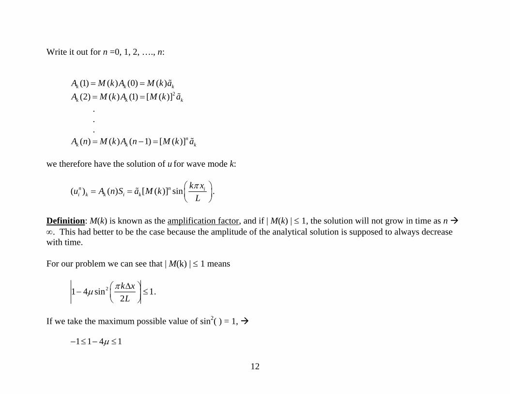
Write it out for n =0, 1, 2, …., n:
(1) ( ) (0) ( )k k kA M k A M k a= = 2(2) ( ) (1) [ ( )]k k kA M k A M k a= =
.
.
. ( ) ( ) ( 1) [ ( )]n
k k kA n M k A n M k a= − = we therefore have the solution of u for wave mode k:
( ) ( ) [ ( )] sinn n ii k k i k
k xu A n S a M kLπ⎛ ⎞= = ⎜ ⎟
⎝ ⎠.
Definition: M(k) is known as the amplification factor, and if | M(k) | ≤ 1, the solution will not grow in time as n ∞. This had better to be the case because the amplitude of the analytical solution is supposed to always decrease with time. For our problem we can see that | M(k) | ≤ 1 means
21 4 sin 12k xL
πμ Δ⎛ ⎞− ≤⎜ ⎟⎝ ⎠
.
If we take the maximum possible value of sin2( ) = 1,
1 1 4 1μ− ≤ − ≤
13
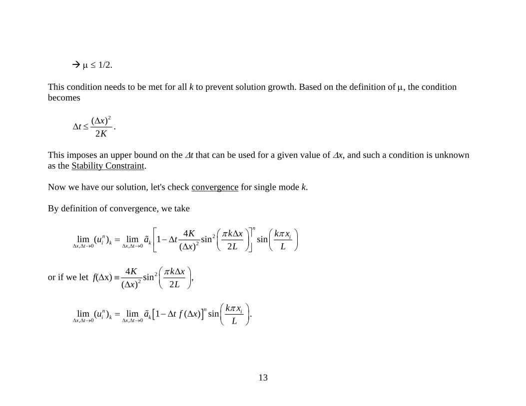
μ ≤ 1/2.
This condition needs to be met for all k to prevent solution growth. Based on the definition of μ, the condition becomes
2( )2
xtK
ΔΔ ≤ .
This imposes an upper bound on the Δt that can be used for a given value of Δx, and such a condition is unknown as the Stability Constraint. Now we have our solution, let's check convergence for single mode k. By definition of convergence, we take
22, 0 , 0
4lim ( ) lim 1 sin sin( ) 2
nn ii k kx t x t
K k x k xu a tx L L
π πΔ Δ → Δ Δ →
⎡ ⎤Δ⎛ ⎞ ⎛ ⎞= − Δ ⎜ ⎟ ⎜ ⎟⎢ ⎥Δ ⎝ ⎠ ⎝ ⎠⎣ ⎦
or if we let f(Δx) ≡ 22
4 sin( ) 2
K k xx L
π Δ⎛ ⎞⎜ ⎟Δ ⎝ ⎠
,
[ ], 0 , 0lim ( ) lim 1 ( ) sinnn i
i k kx t x t
k xu a t f xLπ
Δ Δ → Δ Δ →
⎛ ⎞= − Δ Δ ⎜ ⎟⎝ ⎠
.
14
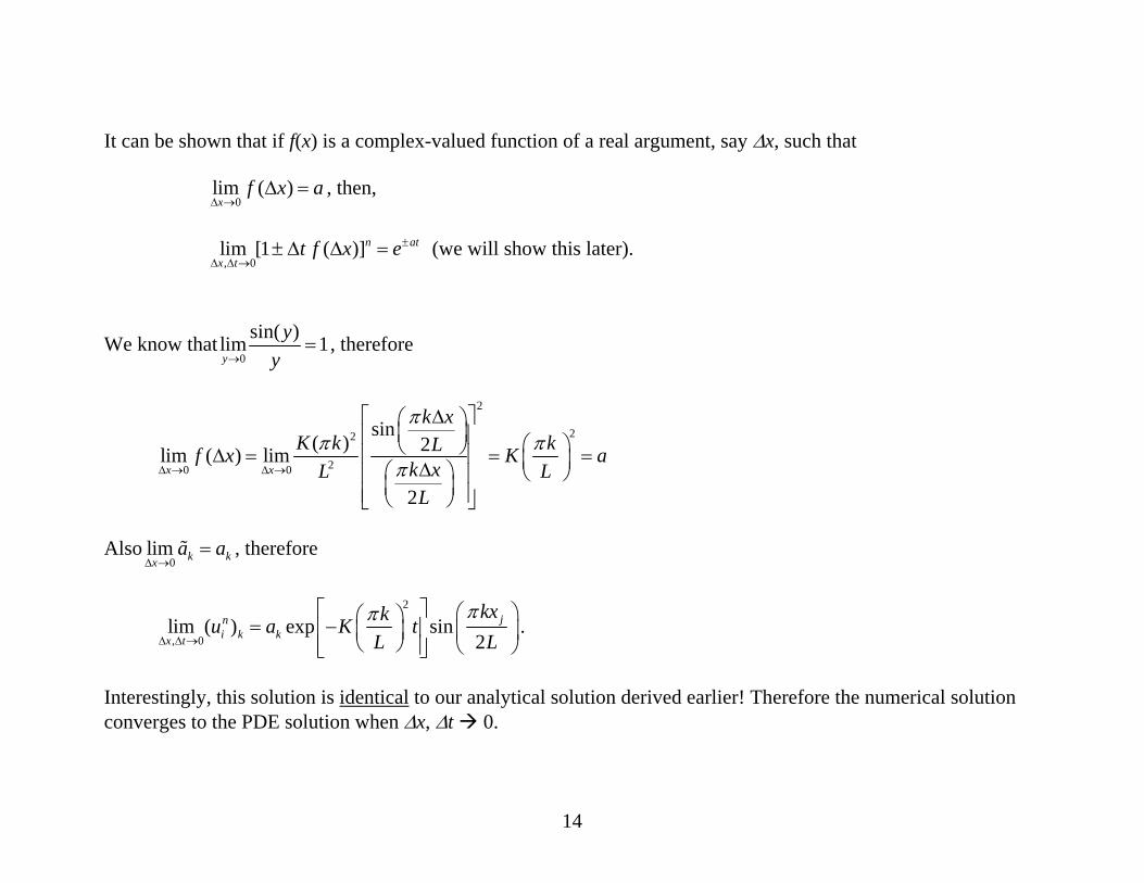
It can be shown that if f(x) is a complex-valued function of a real argument, say Δx, such that
Interestingly, this solution is identical to our analytical solution derived earlier! Therefore the numerical solution converges to the PDE solution when Δx, Δt 0.
2.3.4. Numerical Convergence Reading: Fletcher (handout), Sections 4.1.2, 4.2.1, 4.4.1. Numerical Convergence Convergence is often hard to demonstrate theoretically. True analytical solution is hard or even impossible to find is one of the reasons. We can, however, find out the convergence of a given scheme numerically. We compute solutions at successively higher resolutions and see how the error changes with the resolution.
Does τ 0 when Δx 0?
16
And how fast τ decreases? The procedure can be very expensive (remember the cost factor increase as Δ doubles). A typical measure of error is the L2 norm or RMS error:
2[ ]2 i x iu uLn
Δ −= ∑
where u is a true solution or a 'converged' numerical solution when exact solution is not available. Example: 1-D diffusion equation using FTCS scheme:
Table 4.1 (from Fletcher) shows the error reduction with Δx for two values of s.
The above figure shows plots of log10(err) as a function
of log10(Δx).
18
Recall that
τ = A (Δx)n
log τ = log A + n log Δx. This is a straight line in log-log diagram with a slope of n and intercept A. Thus the slope of the line gives the rate of convergence. In the above figure, we see that when s = 1/6, the error line has a steeper slope and the error is smaller for all Δx. This is because for this value of s, the first term in τ drops out and the scheme because 4th-order accurate. The scheme is second-order accurate for all other values of s. Note that you can choose Δx and Δt such that s=1/6 only when K is constant in the entire domain. In cases where no exact solutions is available, a so-called 'grid-convergence' or reference solution is often sought and this solution can be used in the place of true solution in the estimating the solution error.
19
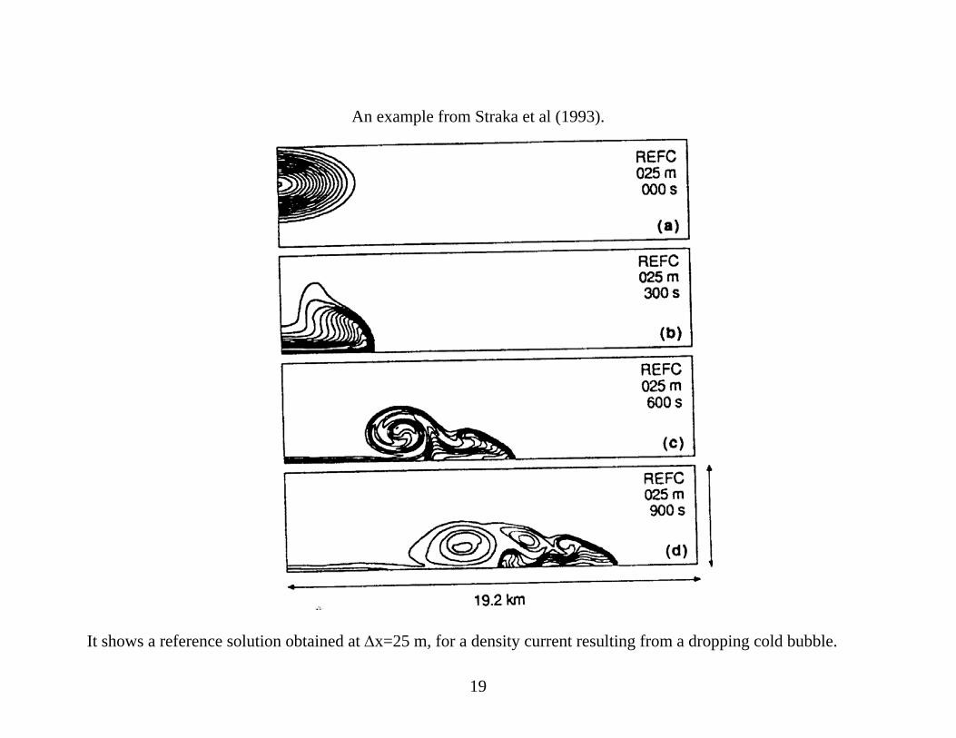
An example from Straka et al (1993).
It shows a reference solution obtained at Δx=25 m, for a density current resulting from a dropping cold bubble.
20
Figure (from Straka et al 1993). Graph of θ' L2 norms (°C) from self-convergence tests with the compressible reference model (REFC). The bold solid line labeled with 'self-convergence solutions' represents the L2 norms for spatial truncation errors of solutions made with Δt = constant and varying grid spacings. The L2 norms were computed against a 25.0 m reference solution. The bold dashed lines labeled with, for example, '200.0 m solutions' represent L2 norms for temporal truncation errors of solutions made with Δx =constant (e.g. 200.0 m) and varying time steps. The reference solutions for these computations were made using a time step consistent with Δt = 12.5 s times a constant in each of the cases. The solid fines labeled O(l) and O(2) represent first- and second-order convergence, respectively.
21
Richardson Extrapolation As the grid becomes very fine, the error behaves much like that predicted from the leading terms in τ. Further refinements are expensive, so we use another technique to improve the solution – Richardson Extrapolation. Consider two numerical solutions obtained at Δxa and Δxb. With FTCS scheme (assuming s ≠ 1/6),
2 44 2
4
( ) 1 ( )2 6
aa a
K x us O x tx
τ Δ ∂⎛ ⎞= − + Δ + Δ⎜ ⎟ ∂⎝ ⎠
2 4
4 24
( ) 1 ( )2 6
bb b
K x us O x tx
τ Δ ∂⎛ ⎞= − + Δ + Δ⎜ ⎟ ∂⎝ ⎠
Find a linear combination of the two solutions, ua and ub
uc = a ua + b ub where a + b =1 and a and b are chosen so that the leading terms in τa and τb cancel and the scheme becomes 4th-order accurate (Of course this assumes that 4 4u x∂ ∂ is the same in both case, which is reasonably assumption only at relatively high resolutions when the solution is well resolved). If Δxb = Δxa/2, then 4a + b = 0 with a + b = 1 a = -1/3, b = 4/3 and uc = -1/3 ua + 4/3 ub.
22
2.3.5. Stability Analysis Reading: Tannehill et al. Section 3.6.
Stability – For a stable numerical scheme, the errors in the initial condition will not grow unboundedly with
time. In this section, we discuss the methods for determining the stability of F.D. schemes. This is very important when
designing a F.D. scheme and for understanding its behavior. There are several methods:
• Energy method • von Neumann method • Matrix method (for systems of equations) • Discrete perturbation method (will not discuss)
Note: Stability refers to the F.D. Does not involve B.C. or I.C. Refers to time-matching problems only The energy method Read Durran Section 2.2 (handout, see web link)
23
This method is used much less often than the von Neumann method. It's attractive because it works for nonlinear problem and problems without periodic B.C. The key is to show that a positive definite quantity like 2( )n
ii
u∑ is bounded for all n.
We illustrate this method using the upstream-forward scheme for wave (advection) equation 0u uct x
∂ ∂+ =
∂ ∂:
1
1 0n n n ni i i iu u u uc
t x
+−− −
+ =Δ Δ
Let μ = cΔt/Δx
11(1 )n n n
i i iu u uμ μ+−= − +
Squaring both sides and summing over all grid points:
1 2 2 2 2 21 1( ) [(1 ) ( ) 2(1 ) ( ) ]n n n n n
i i i i ii i
u u u u uμ μ μ μ+− −= − + − +∑ ∑ (1)
Assuming periodic B.C.
2 21( ) ( )n n
i ii i
u u −=∑ ∑
and using the Schwarz inequality (which says that for two vectors U and V, | | | | | |U V U V⋅ ≤ ⋅ ),
24
2 2 2
1 1( ) ( ) ( )n n n n ni i i i i
i i i iu u u u u− −≤ =∑ ∑ ∑ ∑ .
If (1 ) 0μ μ− ≥ , all coefficients of RHS terms in (1) are positive and we have
1 2 2 2 2 2( ) [(1 ) 2(1 ) ] ( ) ( )n n ni i i
i i i
u u uμ μ μ μ+ ≤ − + − + =∑ ∑ ∑ ,
i.e., the L2 norm at n+1 is no greater than that at n, therefore the scheme is stable! The condition (1 ) 0μ μ− ≥ gives μ = c Δt/Δx ≤ 1 which is the stability condition for this scheme. As we discussed earlier, it says that waves cannot propagate more than one grid interval during one Δt in order to maintain stability. von Neumann method Read Tannehill et al, Section 3.6.1. In a sense, we have already used this method to find stability of the 1-D diffusion equation – when we were proving the convergence of the solution using FTCS scheme. We found then
un+1 = [ M(t) ]n+1 u0
25
where M(t) = amplification factor. If M(t) ≤ 1 by some measure (M can be a matrix or a complex number), then un+1 ≤ un and the solution cannot grow in time – the scheme is stable. Essentially, von Neumann method expands the F.D.E. in a Fourier series, finds the amplification factor and determines under what condition the factor is less than or equal to 1 for stability. Assumptions: 1. The equation has to be Linear with constant coefficients. 2. It is assumed that the solution is periodic. With this method, the dependent variable is decomposed into a complex (or a real) Fourier series:
, ,( , , , ) ( , , )exp[ ( )]
k l mu x y z t U k l m i kx ly mz tω= + + −∑ (2)
where U is the complex amplitude and ω = ωR + i ωΙ is the complex frequency. In fact ωR gives the wave propagation speed and ωΙ gives the growth and decaying rate.
[ ]R I R Ii i t i t ti te e e eω ω ω ωω − + −− = =
Ri te ω− - phase function of Fourier components I teω - growth or decay rate
26
If ωI >0, the solution will grow exponentially in time. Example 1: 1-D diffusion equation with FTCS scheme.
11 1( 2 )n n n n n
i i i i iu u u u uμ+− +− = − + (3)
where 2( )K t
xμ Δ
=Δ
.
Let's examine a single wave k:
( )n i kx ti ku U e ω−=
1 ( )n i kx t i ti ku U e eω ω+ − − Δ=
( )1
n i kx t ik xi ku U e eω− ± Δ± =
Substitute the above into (3)
( ) ( )( 1) [ 2 ]i kx t i t i kx t ik x ik xk kU e e U e e eω ω ωμ− − Δ − Δ − Δ− = − +
( )[ 1 2 (cos 1)] 0i kx t i t
kU e e k xω ω μ− − Δ − − Δ − =
( ) 2[ 1 4 sin ( / 2)] 0i kx t i tkU e e k xω ω μ− − Δ − + Δ =
For non-trivial solution, we require
27
21 4 sin ( / 2) 0i te k xω μ− Δ − + Δ =
21 4 sin ( / 2)i te k xω μ− Δ = − Δ
Here, i te ω− Δ is actually the amplification factor, the same as the M discussed earlier.
i te ωλ − Δ≡ = un+1/un - the amplification factor. For stability we require | λ | ≤ 1
21 1 4 sin ( / 2) 1k xμ− ≤ − Δ ≤ μ ≤ 1/2 as before!
In practice, when μ=1/2, the solution (amplification factor) switches between –1 and +1 for 2Δx waves ( 2sin ( / 2) 1k xΔ = ) very other step, which is unrealistic. The standard requirement is therefore
μ ≤ 1/4. Therefore, do not naively think diffusion terms in a numerical model does not cause numerical instability! When integrated stably, the diffusion term in CFD models tends to stabilize the solution by killing off/damping small scale waves, but when stability condition is not met, it tem itself will cause problem! Read Pielke (1984) section 10.1.2 (handout, see web link).
28
Shorthand notations for discrete/finite difference operators and discretization identities Notations:
/2 /2
2j n j nnx A A
A + −+=
/ 2 / 2j n j nnx
A Ax
n xδ + −−
=Δ
1j jx
A Ax
xδ +
+
−=
Δ
1j jx
A Ax
xδ −
−
−=
Δ
Identities: 2
xxx x xA A Aδ δ δ≡ ≡
( )
xxx x xA B A B B Aδ δ δ≡ −
2( / 2)x
x xA A Aδ δ≡
29
2.3.6. Implicit Methods Read Tannehill et al, second part of section 3.4.1. So far, we have dealt with only explicit schemes which have the form of
1 1( , ,...)n n nu f u u+ −= . With these schemes, the future state at each grid point is only dependent on the current and past time levels, therefore the solution can be obtained directly or explicitly. c.f., explicit functions such as y = x2. Implicit scheme involves variables of the future time level at more than one grid point (often resulting from finite difference of variable(s) at the future time level). Mathematically it can be expressed as
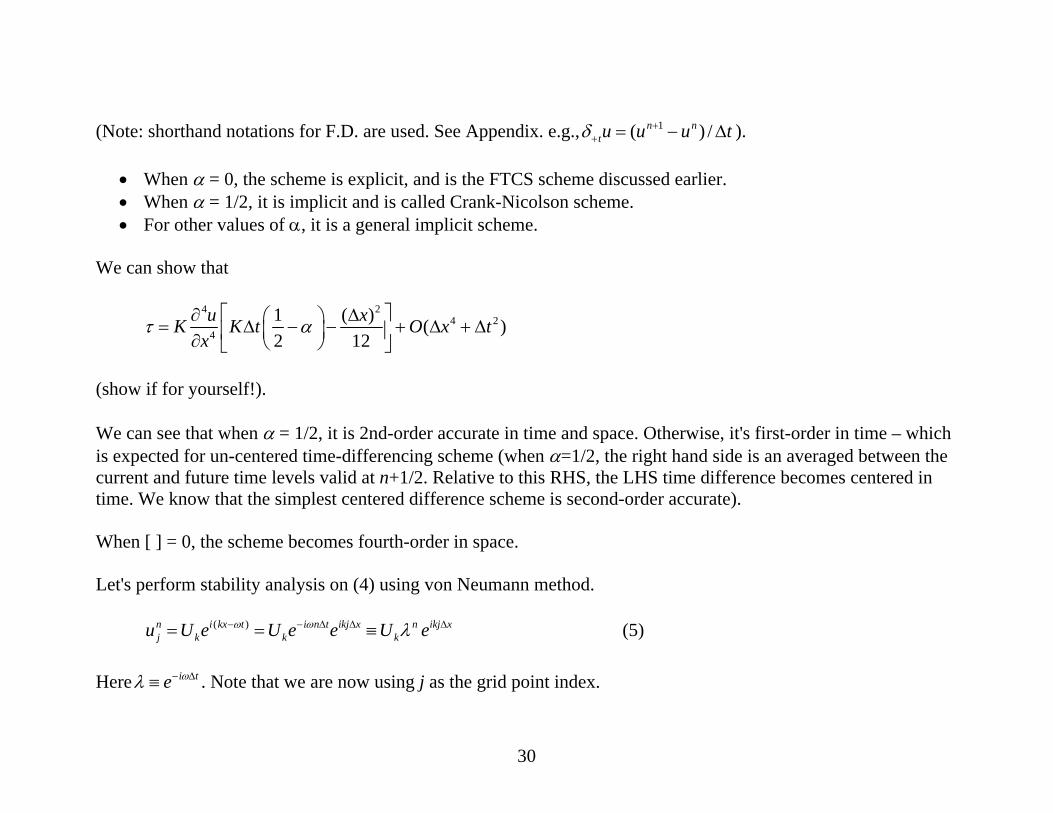
1 1 1( , , ,...)n n n nu f u u u+ + −= . This is analogous to implicit functions such as x = sin(x). As one can imagine, implicit schemes are more difficult to solve. Usually matrix inversion is involved. We will first look at the stability property of an implicit scheme. Example. Consider the 1-D diffusion equation ut = K uxx again. It is approximated by the following F.D. scheme:
1[ (1 ) ]n nt i xx i xx iu K u uδ αδ α δ+
+ = + − (4)
30
(Note: shorthand notations for F.D. are used. See Appendix. e.g., 1( ) /n n
tu u u tδ ++ = − Δ ).
• When α = 0, the scheme is explicit, and is the FTCS scheme discussed earlier. • When α = 1/2, it is implicit and is called Crank-Nicolson scheme. • For other values of α, it is a general implicit scheme.
We can show that
4 24 2
4
1 ( ) ( )2 12
u xK K t O x tx
τ α⎡ ⎤∂ Δ⎛ ⎞= Δ − − + Δ + Δ⎜ ⎟⎢ ⎥∂ ⎝ ⎠⎣ ⎦
(show if for yourself!). We can see that when α = 1/2, it is 2nd-order accurate in time and space. Otherwise, it's first-order in time – which is expected for un-centered time-differencing scheme (when α=1/2, the right hand side is an averaged between the current and future time levels valid at n+1/2. Relative to this RHS, the LHS time difference becomes centered in time. We know that the simplest centered difference scheme is second-order accurate). When [ ] = 0, the scheme becomes fourth-order in space.
Let's perform stability analysis on (4) using von Neumann method.
( )n i kx t i n t ikj x n ikj xj k k ku U e U e e U eω ω λ− − Δ Δ Δ= = ≡ (5)
Here i te ωλ − Δ≡ . Note that we are now using j as the grid point index.
31
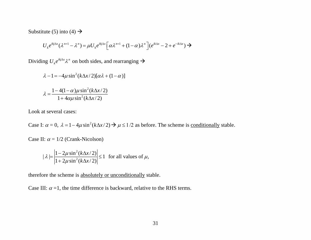
Substitute (5) into (4)
1 1( ) (1 ) ( 2 )ikj x n n ikj x n n ik x ik xk kU e U e e eλ λ μ αλ α λΔ + Δ + Δ − Δ⎡ ⎤− = + − − +⎣ ⎦
Dividing ikj x n
kU e λΔ on both sides, and rearranging
21 4 sin ( / 2)[ (1 )]k xλ μ αλ α− = − Δ + −
2
2
1 4(1 ) sin ( / 2)1 4 sin ( / 2)
k xk x
α μλαμ
− − Δ=
+ Δ
Look at several cases: Case I: α = 0, 21 4 sin ( / 2)k xλ μ= − Δ μ ≤ 1/2 as before. The scheme is conditionally stable. Case II: α = 1/2 (Crank-Nicolson)
2
2
1 2 sin ( / 2)| | 11 2 sin ( / 2)
k xk x
μλμ
− Δ= ≤
+ Δ for all values of μ,
therefore the scheme is absolutely or unconditionally stable. Case III: α =1, the time difference is backward, relative to the RHS terms.
32
2
1| | 11 4 sin ( / 2)k x
λμ
= ≤+ Δ
, again for all values of μ,
therefore the scheme is also absolutely stable. However, this scheme is only first-order accurate in time, as discussed earlier (consistent with the time difference scheme being un-centered). In general, when 0 ≤ α < 1/2, it is required that μ ≤ 1/(2 - 4α ), therefore the scheme is conditionally stable. When 1/2 ≤ α ≤ 1, the scheme is unconditionally stable (it is sometimes referred to as the forward-biased scheme). In the ARPS, the implicit diffusion scheme is an option for treating the vertical turbulent mixing terms. This treatment is necessary in order to remove the severe stability constraint from these terms when vertical mixing is strong inside the planetary boundary layer (PBL). The latter occurs when the PBL is convectively unstably and the non-local PBL mixing is invoked with the Sun and Chang (1986) parameterization. Parameter alfcoef in arps.input corresponds to 1-α here (see handout). Finally, we note that for multi-time level schemes, there is usually multiple solutions for the amplification factor λ. some of them might represent spurious computational modes due to the use of extra (artificial) initial conditions. The expression of λ can be too complicated so that a graphic plotting is needed to understand its dependency on wave number k. |λ| has to be no greater than 1 for all possible waves. The shortest wave resolvable on a grid has a wavelength of 2 Δ, and the longest is 2L, where L is the domain width.
33
Tridiagonal Solver 1-D implicit method often leads to tridiagonal systems of linear algebraic equations. (In the ARPS, this appears twice – once when sound waves are treated implicitly in the vertical direction and once when the vertical turbulence mixing is treated implicitly). For example, Eq. (4) can be rewritten as
1 1 1 11 1 1 1
2 2
2 2(1 )n n n n n n n ni i i i i i i iu u u u u u u uK K
t x xα α
+ + + +− + − +− − + − +
= + −Δ Δ Δ
(6)
It can be rearranged into
1 1 1 1
1 1 1 12 2( 2 ) (1 ) ( 2 )n n n n n n n ni i i i i i i i
tK tKu u u u u u u ux x
α α+ + + +− + − +
Δ Δ− − + = − − + +
Δ Δ
1 1 1
1 12 2 2(1 2 )n n n ni i i i
tK tK tKu u u dx x x
α α α+ + +− +
Δ Δ Δ− + + − =
Δ Δ Δ.
where 1 12
2(1 )n n n
n ni i ii i
u u ud t K ux
α − +− += Δ − +
Δ.
Let 2i itKA Cx
αΔ= = −
Δ, 2
2(1 )itKB
xαΔ
= +Δ
, we then have
1 1 1
1 1n n n n
i i i i i i iAu B u C u d+ + +− ++ + = , (7)
34
for i = 1, 2, …, N-1, assuming the boundaries are at i =0 and N. If we have Dirichlet boundary conditions, i.e., u at i=0 and N are known, then for i =1, the equation becomes
1 1 11 1 1 2 1 1 0
n n n nB u C u d Au+ + ++ = − (8) and for i = N, the equation is
1 1 11 2 1 1 1 1
n n n nN N N N N N NA u B u d C u+ + +
− − − − − −+ = − . (9) For i = 2, 3, …., N-2, the equation remains of the form in Eq.(7). If we write the equations (7-9) in a matrix form, we have
If we have Neumann boundary conditions, i.e., we know the gradient of u at the boundaries which in discretized form are 1 0u u L− = and 1N Nu u R−− = . Plug these relations into Eq.(7) for i=1 and i=N-1, we obtain equations similar to (8) and (9):
1 11 1 1 1 2 1 1( ) n nA B u C u d A L+ ++ + = + (11)
1 11 2 1 1 1 1 1( )n n
N N N N N N NA u B C u d C R+ +− − − − − − −+ + = − . (12)
In this case, the final coefficients in (10) are different for the first and last equation. Since in each except for the first and last row of the coefficient matrix, only three elements are non-zero and the non-zero elements of the matrix are aligned along the diagonal axis, this system is called tridiagonal system of equations. It can be solved efficiently using Thomas Algorithm. The procedure consists of two parts. First, Eq. (7) is manipulated into the following form:
in which the sub-diagonal coefficients A are eliminated and the diagonal coefficients are normalized. For the first equation
1 11 1
1 1
' , 'C DC DB B
= = . (14a)
For the general equations:
1
1 1
'' , '' '
i i i ii i
i i i i i i
C D A DC DB AC B AC
−
− −
−= =
− − for i=2, …, N-1. (14b)
Equations in (14) represent a forward sweep step (see figure below). It is followed by a backward substitution step that finds solution ui from (13). The solution is:
1 1
1
'' ' for from 2 to 1.
N N
i i i i
u Du D u C i N
− −
+
=
= − − (15)
37
Note both (14) and (15) involve reduction, the algorithm is inherently non-parallelizable. Fortunately, for multi-dimensional problems, multiple systems of equations often need to be solved, and one can exploit parallelism along other dimensions (e.g., j instead of i direction). Read Section 4.3.3 of Tannehill et al and Appendix A.
38
2.3.7. Stability Analysis for Systems of Equations When we are dealing with a system of equations, we can also apply the von Neumann method to find the stability property of a given F.D. scheme. As with single equations, von Neumann can only be used for linear systems of equations. For nonlinear systems, linearization has to be performed first. Without going into details, we point out that a system of linear equations can be expressed in a matrix form like
0t x
∂ ∂+ =
∂ ∂u uA (16)
The equation is first discretized using certain F.D. scheme, u can be written in terms of a discrete Fourier series and the wave component is then substituted into the discrete equation to obtain something like:
1 ( , )n nk kt x+ = Δ ΔU M U (17)
where n
kU is the amplitude vector for wave k at time level n, and M is called the amplification matrix. The scheme is stable when the maximum absolute eigenvalue of M is no greater than 1. Why the maximum absolute eigenvalue? Because as you saw earlier (in Chapter 1) that a system of equation like (17) can be transformed into a system of decoupled equations, and the eigenvalues of M become the amplification factors for each of the new dependent variables, vi (the element of vector V), i.e., we can obtain from (17)
39
1n n
k k+ =V N V ,
where N is a diagonal matrix with the eigenvalues of M as its diagonal elements.
T-1 M T = N
1 1 1 1n nk k
− + − −=T U T MTT U Let 1n n
k k−=V T U , we have
1n n
k k+ =V N V .
Therefore 1( ) ( )n n
i k i i kv vλ+ = where iλ are the eigenvalues. Since the system is stable only when all dependent variables remain bounded, the absolute value of the maximum eigenvalue has to be no greater than 1. Read section 3.6.2 of Tannehill et al.