236 IEEE JOURNAL OF OCEANIC ENGINEERING, … Coastal Geosciences Division Mine Burial Burial Program...

236 IEEE JOURNAL OF OCEANIC ENGINEERING, VOL. 32, NO. 1, JANUARY 2007

Progress on Nonlinear-Wave-Forced SedimentTransport Simulation

Richard W. Gilbert, Emily A. Zedler, Stéphan T. Grilli, and Robert L. Street

Abstract—In this paper, we report on the use of a numerical wavetank (NWT), based on fully nonlinear potential flow (FNPF) equa-tions, in driving simulations of flow and sediment transport aroundpartially buried obstacles. The suspended sediment transport ismodeled in the near-field in a Navier–Stokes (NS) model using animmersed-boundary method and an attached sediment transportsimulation module. Turbulence is represented by large eddy sim-ulation (LES). The NWT is based on a higher order boundaryelement method (BEM), with an explicit second-order time step-ping. Hence, only the NWT boundary is discretized. The solutionfor the velocity potential and its derivatives along the boundaryis obtained in the BEM, which subsequently provides a solutionat any required internal point within the domain. At initial time,the NS–LES model domain is initialized with the 3-D velocity fieldprovided by the NWT and driven for later time by the pressuregradient field obtained in the NWT. Incident wave fields, as spec-ified in the NWT to drive sediment transport, can be arbitrary.Applications are presented here for single frequency waves, suchas produced by a harmonic piston wavemaker in the laboratory,and modulated frequency wave groups. The feasibility of couplingthe irrotational flow and NS solutions is demonstrated.

Index Terms—Boundary element method (BEM), coastal pro-cesses, computational fluid dynamics, model coupling, nonlinearwaves, sediment transport.

I. INTRODUCTION

I N this paper, we report on our progress towards the modelingof wave-induced flow and suspended sediment transport

around partially buried cylindrical obstacles, using a coupledwave-hydrodynamic-sediment transport model. While mostsimilar work to date has usually been based on specifying asimple oscillatory flow to force the sediment transport [1]–[4],

Manuscript received March 31, 2005; revised April 4, 2006; accepted June29, 2006. This work was supported by the U.S. Office of Naval Research(ONR) Coastal Dynamics Program under Grant N00014-00-1-0440 and theONR Coastal Geosciences Division Mine Burial Burial Program under GrantN00014-05-1-0068 (code 321CG).

Guest Editor: M. D. Richardson.R. W. Gilbert was with the Department of Ocean Engineering, University of

Rhode Island, Narragansett, RI 02882 USA. He is now with the McLaren En-gineering Group, West Nyack, NY 10994 USA (e-mail: [email protected]).

E. A. Zedler was with the Environmental Fluid Mechanics Laboratory, De-partment of Civil and Environmental Engineering, Stanford University, Stan-ford, CA 94305 USA. She is now with the Santa Clara Valley Water District,San Jose, CA 95118 USA (e-mail: [email protected]).

S. T. Grilli is with the Department of Ocean Engineering, University of RhodeIsland, Narragansett, RI 02882 USA (e-mail: [email protected]).

R. L. Street is with the Environmental Fluid Mechanics Laboratory, Depart-ment of Civil and Environmental Engineering, Stanford University, Stanford,CA 94305 USA.

Color versions of one or more of the figures in this paper are available onlineat http://ieeexplore.ieee.org.

Digital Object Identifier 10.1109/JOE.2007.890979

here, we use the more realistic background wave velocityfield created by fully nonlinear waves, both over flat bottomand shoaling over slopes. Earlier research indeed shows thatnonlinear effects in shoaling wave fields lead to asymmetries inboth wave shape and near-bottom currents that strongly affectsediment transport (e.g., [5]–[9]) and the resulting burial orunburial of obstacles located on the bottom.

When approaching shore, due to refraction, shoaling oceanswells often become locally 2-D in the cross-shore direction.A 2-D waveform is thus a good approximation for simulatingwave-induced sediment transport in an essentially cross-shoredirection (e.g., Fig. 1). Recent laboratory experiments per-formed in a wave tank with moving bottom at the ArizonaState University (ASU, Tempe, AZ, [5], [6], [8]–[10]) showthat small scale disturbances in the bottom topography, as com-pared to the wavelength, such as sand ripples or small partiallyburied obstacles, usually affect flow velocities only within 2–3significant diameters of the object and have negligible effectson the waveform. This allows us to simulate the 2-D wave“far-fields,” to provide background wave velocities for drivingthe 3-D turbulent flow that occurs around bottom obstacles, inthe “near-field.”

We model far-field waves in a 2-D numerical wave tank(NWT), solving fully nonlinear potential flow (FNPF) equa-tions, based on a higher order boundary element method (BEM)and an explicit time stepping [7]–[9], [11]–[14]. The potentialflow approximation (i.e., irrotational motion of an inviscid,incompressible fluid) used in this NWT has been shown inearlier work to be very accurate for simulating both the shapeand velocities of shoaling waves, as compared to laboratorymeasurements (e.g., [7], [8], and [15]–[17]). Figs. 1 and 2,for instance, show the setup, and then, the results of a recentcomparison of simulations in this 2-D–NWT, with laboratoryexperiments at ASU [8], [9]. We see that both the simulatedperiod-averaged wave elevation close to breaking and thenear-bottom horizontal velocity are in good agreement withmeasurements. Discrepancies of only a few percent beforebreaking are typical.

Here, the 2-D–NWT is similarly used to simulate wavegeneration, propagation over a flat bottom, and transformations(i.e., shoaling) over a sloping bottom topography, and corre-sponding wave-induced internal velocities and pressure fields.These serve as both initialization and background forcing, asa function of time, for a near-field 3-D Navier–Stokes (NS)hydrodynamic model. At this time, no feedback of NS modelresults into the NWT is implemented. This so-called “weakmodel coupling” approach was successfully applied in earlierwork to the modeling of shoaling, breaking, and postbreakingwaves, by using a 2-D- or a 3-D–FNPF–NWT to initialize and

0364-9059/$25.00 © 2007 IEEE

GILBERT et al.: PROGRESS ON NONLINEAR-WAVE-FORCED SEDIMENT TRANSPORT SIMULATION 237

Fig. 1. Sketch of the 2-D–NWT setup for computations of wave shoaling and breaking over a sandy slope S = 1 : 24. Note that AB is absorbing beach for x � x ;a piston wavemaker is located at x = x ; and ( ) indicates the position of the sand layer in the laboratory wave tank used at ASU, for which dimensions arein meters [8], [9]. In these experiments, there was a 8.4-cm radius, 50% buried cylinder at x = 12.8 m.

Fig. 2. Example of comparison of the 2-D–NWT computations to laboratoryexperiments (�), from [8] and [9] for the case of Fig. 1 without the bottom ob-stacle, for x = 12.8 m (i.e., just before the AB). Results show period averaged:(a) surface elevation �; (b) horizontal velocity u ( ) and vertical velocity w(� � �) at 0.1 m above the bottom.

drive a 2-D- or 3-D–NS model, with a free surface describedby the volume of fluid (VOF) method [18]–[21].

In the NWT, waves can be generated either by a numericalwavemaker, such as used in laboratories, or as actual fullynonlinear waves. An absorbing beach is specified at the otherextremity of the NWT, to dissipate incident wave energybefore wave overturning and breaking occur [14]. In the NSmodel, turbulence is represented by large eddy simulation(LES) and sediment transport is computed by a suspendedsediment transport model. Although wave computations are2-D, the NS–LES model is 3-D and implemented over a smallernear-field computational domain than the NWT (e.g., Figs. 3and 4), where wave-induced suspended sediment transportis calculated. Resolved-scale turbulence, which accounts fora majority of sediment transport, is represented in the 3-Deddies that are simulated in the NS–LES model. Subgrid scaleturbulence is represented by an eddy viscosity model. In thesediment transport module, suspended sediment transport issimulated with an advection–diffusion scheme, forced by thewave-induced velocity field from the NS–LES model.

The NWT, NS–LES, and sediment transport models are de-scribed in Sections II-A and II-B. This includes a summary ofgoverning equations, boundary conditions, and an overview of

numerical methods for each model. In a first application, wesimulate the generation of an incident wave group through mod-ulating a periodic wave train and its shoaling over a mild slope.This is to illustrate the capabilities of the NWT to simulate thedevelopment of irregular and highly nonlinear waveforms, suchas occurs for ocean swells. In a second application, we illus-trate our coupled approach with the NWT, NS–LES, and sedi-ment transport models, by generating 2-D periodic waves over aflat bottom and driving sediment transport, in the 3-D near-fieldNS–LES domain, around a 75% buried cylindrical object (rep-resenting a mine).

Results for the wave fields generated and the sediment trans-port modeled are discussed in this paper.

II. BACKGROUND OF NUMERICAL MODELS

The fully nonlinear 2-D–NWT used in this paper is basedon a potential flow approximation, thus assuming irrotationalflows of an incompressible, inviscid fluid. Many earlier studiesand comparisons with experiments confirm the validity ofthis model-to-model highly nonlinear wave transformationsin coastal areas [7]–[9], [15]–[17]. The 3-D–NS–LES modelhas been successfully applied to the computation of turbulentboundary layer and separated flows over ripples, induced byoscillatory currents (e.g., [1] and [2]).

Next, we separately summarize the equations of these twomodels, and of the sediment transport model, and then, explainhow the three models were combined to address the problem ofsediment transport induced by shoaling waves.

A. Governing Equations and Boundary Conditions

1) Numerical Wave Tank: Equations for the 2-D–NWT arebriefly presented in the following (see [8] and [11]–[14], for de-tails). The velocity potential is introduced in the verticalplane and the velocity is defined by .Continuity equation in the fluid domain with boundary

is a Laplace’s equation for the potential (Fig. 1)

in (1)

Using Green’s second identity, (1) is transformed into aboundary integral equation (BIE)

(2)


Fig. 3. Typical BEM discretization for a flat bottom case, with a partially buried obstacle, and a periodic wave generation by a piston wavemaker (there is a 5 �vertical exaggeration). Symbol indicates the location of the submerged NS–LES domain.

Fig. 4. Closeup of BEM discretization and NS–LES domain with a 75% buriedobstacle. (�) BEM discretization nodes.

where the Green’s functions are defined as

(3)

with , , , and positionvectors for points on the boundary, the outwardunit normal vector to the boundary, and is a geometriccoefficient function of the exterior angle of the boundary at(usually for a smooth boundary geometry).

a) Boundary conditions: On the free surface , satisfiesthe kinematic and dynamic boundary conditions

on (4)

on (5)

respectively, with the position vector on the free surface,the gravitational acceleration, the vertical coordinate, thefree-surface pressure, and the water density. Along the bottomboundary , a no-flow condition is prescribed as

on (6)

where the overline denotes specified values.From Bernoulli equation (5), the wave-induced dynamic

pressure within , which will force the NS–LES model, isexpressed as

(7)

The computation of the internal solution based on the boundarysolution is explicit in the BEM. Details are given as follows.

b) Wave generation: Various methods have been usedfor wave generation in this NWT. Here, waves are generatedon boundary , as in laboratory experiments, using a solidpiston wavemaker moving according to a prescribed motion

. Thus, we have

on (8)

where the time derivative follows the wavemaker motion. Wave-maker laws are given in the application section. (Note that thepiston motion is usually ramped-up over three representativewave periods, by modulating the stroke using a functionof time. See references for details.)

c) Wave absorption: During shoaling of a periodic waveover a slope and before breaking (which, on a mild slope, ap-proximately occurs when the ratio of waveheight over depth

), wave steepness, and asymmetry (both be-tween trough and crest and between front and rear of each wave;e.g., Fig. 1) continuously increase. This paper focuses on sed-iment transport induced by such highly nonlinear and asym-metric waves, before breaking. Breaking is prevented in theNWT by dissipating incident wave energy in a numerical ab-sorbing beach (AB), located beyond the area of interest (e.g.,Fig. 1).

Following [14], the AB is specified for (Fig. 1). Inthe AB, an external free-surface pressure is applied tothe free surface, by way of the dynamic free-surface condition(5) (with ), to create a negative work and absorb waveenergy. Additional wave reduction is induced by causing wavesto deshoal, using a bottom geometry within the AB somewhatsimilar to a natural bar, with a depth increasing from to

. The AB “absorbing pressure” is specified proportional to thenormal particle velocity on the free surface

(9)

where is the AB absorption function. This function is firstramped-up from 0 to , and then, maintained constant overthe AB. More specifically

(10)

where is a nondimensional beach absorption coefficient, andfollows a variation for and

for .


An absorbing piston (AP; [14]) is also specified at the ex-tremity of the AB, for . This AP moves proportionally tothe hydrodynamic pressure force caused by waves, calculatedas a function of time in the NWT (see references for details).Grilli and Horrillo [14] showed that the combination AB/AP ef-fectively absorbs incident wave energy in the NWT to withinany specified small fraction.

d) Bottom friction: For short distances of propagation overa smooth bottom, wave damping due to bottom friction is quitesmall, and is usually neglected in numerical models, even forlong waves, when the computational domain only spans a fewwavelengths (e.g., [15] and [17]). To simulate wave shoalingover a rippled sandy bed, which may induce more significantwave damping due to bed roughness, Grilli et al. [8] simulatedan energy dissipation term due to bottom friction in the NWT.They did so by specifying a surface pressure distribution, similarto that detailed previously for the AB, over the shoaling regionfor (Fig. 1).

For the initial applications reported here, we did not imple-ment a moving sediment bed and, hence, neglected bottom fric-tion effects on wave shape and velocities. Such effects could,however, be included in a later time. More details regardingbottom friction can be found in [9].

e) Solution for internal fields: At each time step, the NWTprovides the solution for the velocity potential , its normalderivative , and the time derivative of these [ and

], along-boundary . Potential , for any pointwithin domain , can then be explicitly calculated based on theboundary solution, based on BIE (2), (3), expressed for .

Internal velocity fields are required to initialize the NS–LESmodel, and velocities together with the time derivative of thepotential are needed to calculate the wave-induced internal dy-namic pressure (7). If we denote bythe gradient operator with respect to the coordinates of point

, (2) yields

(11)

and

(12)

where

(13)

(Note that the derivatives with respect to internal point coordi-nates have been directly applied to the Green’s functions in theintegrand.)

Similarly, internal dynamic pressure gradient fields, whichwill be used to force the NS–LES model as a function of time,are obtained as

(14)

where the first term in the right-hand side of (14) is obtained byexpressing (12) for and , and the last term,by applying to (12), which yields

(15)where

(16)

in which index notation has been used for convenience, withcorresponding to directions and for 2-D prob-

lems and the Kronecker symbol. (Note that, in accordancewith Euler equation, the bracket in the right-hand side of (14)is in fact equal to the total flow acceleration at point minusgravity.)

2) NS Model: The equations governing fluid motion are con-tinuity and the volume-filtered incompressible NS equations,with the Boussinesq approximation invoked, and a source termfor forcing oscillatory or wave-like motion

(17)

(18)

(19)

Here, is the 3-D velocity ( ), is the subfilter scale(SFS) shear stress term, is the momentum sourceterm for the forcing wave motion, corresponding to the dynamicpressure gradient computed in the NWT using (14)–(16), isthe kinematic viscosity, is the Cartesian coordinate (is vertical), and the overbars denote spatial filtering with a boxfilter. Here, because of the inherent mismatch between the ir-rotational NWT and rotational NS solutions, we elected to useone-way coupling by driving the NS solution with the full dy-namic pressure from the NWT solution and have not forced thevelocities at the NS domain boundary.

The SFS term is represented by the Smagorinsky model, aneddy viscosity model which gives the local eddy viscosityas proportional to the magnitude of the local strain rate tensor

[22]. Namely

(20)

Here, is the grid-filter width and is a flow-dependentmodel coefficient; we use .

a) Boundary conditions: On the inflow/outflow bound-aries and , and along the top of our domain , we specify


a gradient-free condition, i.e., and ,respectively, where (Figs. 3 and 4).

The bottom boundary condition on is no-slip, or ,implemented via the immersed boundary method (IBM).

The lateral boundaries are treated as free slip surfaces, satis-fying , , and .

3) Sediment Transport Model: The suspended sediment con-centration is modeled with a volume-filtered advection–diffu-sion equation

(21)

where sediment concentration by volume fraction andscalar flux term.

Consistent with the common assumption in the literature thatthe turbulent Schmidt number , the same model is adoptedfor the SFS terms for both the momentum and sediment concen-tration equations, i.e., we have used the Smagorinsky model forboth.

a) Boundary conditions: For the inflow/outflow andtop boundaries ( , , and ), we have used gradient-freeboundary conditions (Fig. 4).

For the bottom boundary , we have used an empirical func-tion developed by van Rijn [23] for evaluating the sediment con-centration near the bed, as it varies along the bed

(22)

where the bottom shear velocity is , the critical shear velocityis , and the roughness height is .

To compute , we solved the boundary layer log-lawfor at each location along the

bed, using as inputs the velocity computed from the previoustime step at the grid point nearest to the bed location and thedistance of that point to the bed, where . Nakayamaet al. [24] show that, for smooth wall flows, the filtered (inthe LES sense) instantaneous wall shear stress and velocityat points above the bed correlate well, and that a log-lawrelationship is reasonable. Nakayama [25] confirmed that therelationship holds as well for rough walls. For , we usedvan Rijn’s representation of the Shields curve as a function of

[26, eq. (4.1.1)].Our selection of (22) for predicting the near-bed concentra-

tion was based on the following considerations.• It provides a reference concentration (as opposed to a

pickup rate), which was necessary for this first applicationand use with the IBM (see Section II-B2).

• It has the same form as van Rijn’s pickup function [27],employed in the bottom boundary condition in the sim-ulations over ripples performed by Zedler and Street [1],in that it is proportional to . Since van Rijn’s pickupfunction produced physically realistic transport patterns inthese simulations, it seemed a reasonable place to start.

• While originally developed to predict the spatially aver-aged sediment concentration at the top of dunes, it wasfound to provide the best estimate of concentration at a dis-tance from the bed equal to 5% of the total depth, as com-pared with six other formulas tested against data in Garciaet al. [28].

• Although we apply (22) at the bed, rather than at a dis-tance above it, we have reasons to believe (from previoussimulations) that its basic form (as proportional to a powerof ) produces physically realistic transport patterns. Forquantitative predictions, it will be desirable to introduce aflux-prediction boundary condition, as suggested by Ad-miraal et al. [29] and used by Zedler and Street [30].

Note, in this paper, we were intent on demonstrating the fea-sibility of coupling the irrotational wave forcing, the NS andadvection solutions, and the IBM of representing the bed. Im-plementing a flux boundary condition in the IBM is, as notedpreviously, a nontrivial exercise that is a natural next step be-yond this present effort. In addition, Admiraal et al. [29] citeevidence for a phase-lag between the peak shear stress and thesediment concentration at a given cross section. Indeed, that fea-ture of the transport is particularly evident in Zedler and Street[30]. Our formulation estimates the concentration at the bed inproportion to the shear stress (and while we would prefer to es-timate the flux there, that was not possible at this time in theevolution of our model), and then, calculates the transport ofsediment by advection and turbulent mixing (an LES algorithm)above the bed. Accordingly, based on advection effects alone,sediment concentration peaks above the bed will occur down-stream of the shear stress peaks; thus, the phase-lag mechanismis included in our formulation, but the bed boundary conditionis not ideal.

B. Numerical Methods Used in Models

1) Numerical Wave Tank: The BIE (2) is solved by a BEM,by expressing it for discretization nodes on the boundary( ; ), and defining higher order elementsto interpolate in between discretization nodes. In the presentapplications, quadratic isoparametric elements are used onlateral and bottom boundaries, and cubic elements ensuringcontinuity of the boundary slope are used on the free surface.In these elements, referred to as midcubic interpolation (MII)elements, both geometry and field variables are interpolatedbetween each pair of nodes, using the midsection of a four-node“sliding” isoparametric element. The Green’s function and itsnormal derivative in (3) are singular as . These singular-ities require additional treatments whose detailed derivationswill not be included here. These can be found in [11] and [13]for both isoparametric and MII elements. It should be notedthat, when applying (2) to points that are very close to adifferent part of the boundary (e.g., near corners in Fig. 1),almost-singular integrals will occur when is very small. Thenumerical accuracy of such integrals is improved by applyingan adaptive integration method.

a) Time integration: Free-surface boundary conditions (4)and (5) are time integrated based on two second-order Taylor


series expansions expressed in terms of a time step and ofthe Lagrangian time derivative , for and

(23)

respectively. First-order coefficients in the series correspond tofree-surface conditions (4) and (5), in which and areobtained from the BEM solution of the BIE (2) for ( , )at time . Second-order coefficients are expressed as of(4) and (5), and are calculated using the solution of a secondsimilar BIE for ( , ), for which boundary con-ditions are obtained from the solution of the first BIE and thetime derivative of (5)–(8). Detailed expressions for the Taylorseries coefficients can be found in [11].

At each time step, the overall numerical accuracy is estimatedby computing errors in volume and energy of the computationaldomain. Earlier work showed that these errors are function ofboth the size (i.e., distance between nodes) and the degree (i.e.,quadratic, cubic, etc.) of boundary elements used in the spatialdiscretization, and of the size of the selected time step [12], [13].Thus, the optimal time step is adaptively selected based on amesh Courant number, whose optimal value for MII elementswas shown to be about 0.45. This value is used in the presentapplications.

In computations involving finite amplitude waves, mean driftcurrents occur (“Stokes drift”), which continuously move free-surface discretization nodes/Lagrangian markers away from thewavemaker into the NWT. Hence, when performing compu-tations over many wave periods, nodes are redistributed (i.e.,regridded at constant arclength intervals over the free surface)after fixed numbers of time steps.

b) Solution for internal fields: All of the integrals in (11),(12), and (15) expressing interior fields are nonsingular and canbe evaluated by Gauss quadrature. However, for interior pointslocated very close to boundary , similarly to corner pointsin the original discretized BIE (2) (see [12]), the integral ker-nels will rapidly grow as becomes small, yielding inaccuratenumerical integration over parts of the boundary nearest thosepoints. This is even more so when the operator has been ap-plied to the Green’s functions, as in (13) and (16), where termsare to for small . Grilli and Svendsen [12]and Grilli and Subramanya [31] studied these numerical inte-grations in detail, referred to as quasi-singular integrals (QSI).Following their method, in NWT computations, a geometricalanalysis of the discretization is made at each time step, whereQSIs are identified based on a distance criterion. During nu-merical integration of the various BIEs, both for the boundarysolution and for internal points, QSIs are then integrated usingan adaptive integration method, in which elements are subdi-vided into an increasingly large number of subsegments, as afunction of a distance-based algorithm. The originally selectednumber of Gauss points is used within each subsegment. Grilliand Subramanya [31] showed that, given enough subsegments,

this method can provide almost arbitrary numerical accuracy ofthe QSIs.

2) NS Model: QUICK [32] is used for the spatial discretiza-tion of the advection terms in the momentum (19), and cen-tral differences for all other terms. The same methods are usedfor discretizing the advection–diffusion (21) for the sedimentconcentration field, except that simple high-accuracy resolu-tion program (SHARP) [33] is used in place of quadratic up-stream interpolation for convective kinematics (QUICK) for itsimproved handling of sharp gradients. Both equations employ aCrank–Nicolson averaging for the diagonal viscous terms, andthe Adams–Bashforth method for all other terms, which yieldsa semi-implicit, quasi-tridiagonal system of equations.

This system of equations is solved with a fractional stepmethod. In this method, an estimate of the velocity field is firstobtained by solving NS equations without the pressure term,the pressure Poisson equation is solved for the pressure asdriven by the estimated velocity field, and the velocity estimateis corrected with the pressure to satisfy continuity.

Further details about the equations, discretization, and numer-ical methods can be found in [34] and [35].

a) IBM: Of the many versions of the code originally de-veloped by Zang et al. [34], we employ a modified version ofthe Tseng and Ferziger [35] code, which includes implementa-tion of the IBM via a ghost cell method [35].

The IBM works by applying the force necessary at thelocation of the immersed boundary to enforce the physicalboundary condition, in this case. (The implementationof a log-law in the IBM over a complex boundary is exceedinglydifficult [36] so, as an approximation, we have assumed thatthe boundary lies at the location where the log-law velocityis zero.) In the ghost point method, this involves providing adescription of the immersed boundary shape, identifying thenearest neighbor grid points below (the ghost cells) and above(the interpolating points) the immersed boundary, and usinginterpolation methods to enforce the boundary condition at theimmersed boundary. Values at the ghost point are then set byextrapolation with the interpolation function. Essentially, thisamounts to translating the boundary conditions to the locationof the physical immersed boundary.

In this case, we fit a vertical second-order Lagrange polyno-mial function to the values at the two points above a ghost cell.

III. APPLICATIONS

Applications presented here include the following two cases:1) the simulation of shoaling wave groups in the NWT

(Figs. 6 and 7);2) the simulation of periodic wave flows in the NS–LES

model and induced suspended sediment transport, overa 75% buried cylindrical obstacle on the bottom, repre-senting a mine (Figs. 3–5 and 8–10).

We present the first application (case 1) to illustrate the capa-bilities of the NWT to simulate the shoaling of complex fullynonlinear wave trains. In case 2, results are qualitatively com-pared with those of [1] and [2], obtained for the forcing of theNS–LES and sediment transport models over a rippled bed by asimple oscillatory flow.


Fig. 5. Example of internal velocity field computed in the 2-D–NWT (at timet = 20.03 s after the start of simulations), within a vertical cross section inthe 3-D NS–LES domain, in a geometry similar to that of Figs. 3 and 4, witha 75% buried cylindrical obstacle on the bottom. Note, for clarity, the numberof internal points has been reduced by a factor of 6; c is the theoretical linearwave celerity at depth h .

A. Discretization and Parameters

1) Numerical Wave Tank: Table I gives a summary of waveand BEM discretization parameters used in the NWT for eachapplication presented here. More details are given later.

a) Discretization: Typical free-surface discretizations (on) usually have at least 20 nodes per dominant wavelength

(e.g., Fig. 3). Lateral boundaries ( and ) are typically dis-cretized with only 7–11 nodes. Bottom discretizations (on )are usually a little coarser than on the free surface, but horizontalnode spacing is reduced on the bottom under the NS–LESdomain , to further increase the accuracy of the integralsused to compute internal fields in the BEM solution (Figs. 3–5).Adaptive integrations, with up to subdivisions, are performedwithin four nodes of any corner of the BEM domain, and for allelements located directly under , where points at which in-ternal velocities and pressure gradients are calculated and usedfor model coupling are specified (Fig. 5). Initial time steps areselected based on the free-surface node spacing, to satisfy theoptimal mesh Courant number. Time step is subsequently au-tomatically adjusted as a function of the minimum distance be-tween nodes on the free surface to satisfy the Courant condition.Typical central processing unit (CPU) times in the NWT are lessthan one second per time step on a desktop computer.

b) Dissipation: In these applications, the NWT was runwithout bottom friction, and with no regridding applied on thefree surface, because no long term computations were run in theBEM model at this stage, as only one single representative pe-riod of wave forcing was used to force the NS–LES domain.Longer term computations, for instance with moving bottom(such as migrating ripples), would require regridding the freesurface (see [8] and [9]). An absorbing beach AB and an ab-sorbing piston AP (Fig. 1) were specified in each case, to dampincident wave energy and eliminate wave reflection at the NWTextremity.

TABLE INONDIMENSIONAL WAVE AND NWT PARAMETERS IN APPLICATIONS;! = 2�=T , WHERE T IS PERIOD; h = 0.80 m FOR FLAT BOTTOM

OR 2.62 m FOR WAVE GROUPS DENOTE THE REFERENCE

CONSTANT DEPTH (FIG. 1); g = 9.81 m/s IS ASSUMED

2) NS Model: In case 2, the NS–LES model grid di-mensions are 0.3 m long by 0.1727 m high by 0.0125 mwide (Fig. 4). For the partially buried obstacle, the bottomis flat in the streamwise direction to either side of a cen-tral bump, represented by a 75% buried cylinder of radius0.084 m, whose axis runs in the spanwise direction. TheNS–LES model is discretized by 82 98 6 grid points.Hence, we use 82 98 8036 points in each vertical planeof the 3-D NS–LES domain. The immersed boundary is locatedabove the actual grid boundary so that the total flow domainheight is 0.17 m (discretized by 95 points in the vertical direc-tion over the flat regions). The mine protrudes a vertical dis-tance of 0.042 m into the flow. The wave forcing is 2-D, as isthe bed and, based on our previous work [30], the main struc-ture of the vortices in the vertical plane is not significantly influ-enced by cross-stream resolution in channel flows. Accordingly,we used only a minimum of cross-stream grid points, assumingthat while the flow will not be well resolved in that direction,the results in the vertical plane are not noticeably impacted. Nochange in the model or setup, however, is required to increasethe cross-stream resolution, but the computer time required in-creases rapidly as one does that.

For the coupled simulations with a periodic wave flow, waveforcing is computed in the NWT, within the fixed embeddedNS–LES grid (Figs. 3–5). Thus, the NWT provides the far-fieldvelocities and free-surface wave forcing throughout most of thedomain , while the embedded NS solution provides a well-resolved description of the wave boundary layer within domain

, with no slip enforced at the bed. The computation of theNS–LES model forcing in the application is further discussedlater.

3) Sediment Transport Model: Here, we assume the sedi-ment is sand, with a particle size 200 m, a ratio ofsediment density to fluid density 2.65 (sediment densityis 2650 kg/m ), a roughness height 0.024 m, and a settlingvelocity 0.026 m/s, for sediment of this diameter. Becausethe vertical resolution is not sufficient for quasi-direct NS sim-ulations, and we do assume that the bed is rough, we have usedthe log-law to estimate the shear stress for use in the sedimenttransport simulations (see Section II-A3). This has no effect on


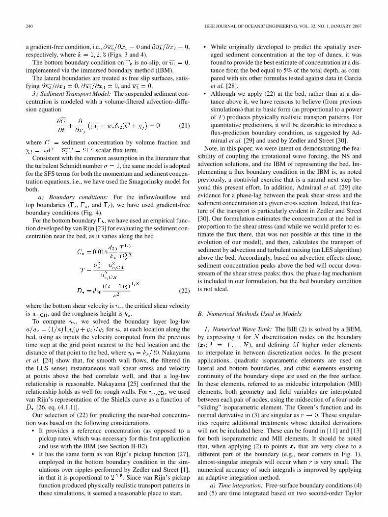
Fig. 6. Case 1: NWT domain used for wave group generation and shoaling over a 1 : 20 slope. The free surface is shown at t = 70 s. The AB is for x > 32 m andh = 2.62 m.

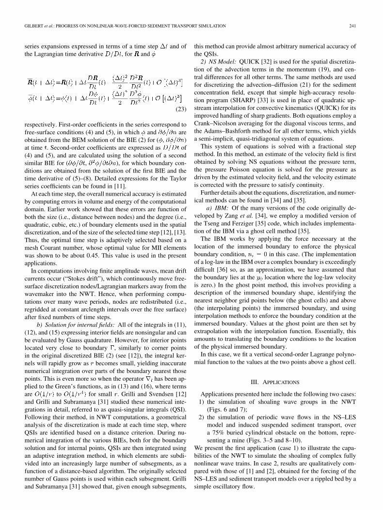
Fig. 7. Case 1: Time series of shoaling wave group (case of Fig. 6), for x being equal to (a) 9.7, (b) 20, and (c) 30 m.

the momentum calculations, but is reasonable as noted in thatsection.

B. NS–LES Flow Forcing by Internal Fields

For the NWT–NS–LES-coupled case 2, wave generation isramped-up over three periods in the NWT and computationsare performed until a quasi-steady regime is reached. This usu-ally takes ten wave periods or so. Internal velocity fields arethen calculated in the NWT using (12) and (13), to initialize theNS–LES model over a grid of points within the small immerseddomain (e.g., Fig. 5). Pressure gradient fields are calcu-lated over the same grid using (14)–(16), for later time steps,to provide the momentum source term in the NS–LES model(19). Thus, the NWT forcing is applied at each grid point of theNS–LES model, in the horizontal and vertical momentum equa-tions, and varies downstream, vertically, and in time. There is noNWT forcing in the transverse direction for this 2-D flow.

More specifically, in the NWT, to avoid having internalpoints located very close to the bottom boundary of ,which would cause severe QSIs in the calculation of internalfields, requiring time consuming element subdivisions, a

smaller number of internal points are used on vertical linescorresponding to the NS–LES grid. These points are placedat equal intervals between the free surface and the bottom ofdomain (e.g., Fig. 5). The internal fields computed at thesepoints are then vertically interpolated, using cubic splines, tothe exact vertical locations of the NS–LES domain grid points.

Internal fields computed in the 2-D–NWT, for grid points inthe vertical plane, are then copied uniformly to each verticalgrid in the third dimension of the 3-D NS–LES domain. Initialvelocities are thus assumed 2-D when passed from the NWTto the NS–LES model, i.e., with , and for later timesteps, internal pressure gradients forcing the NS–LES model arealso assumed 2-D, with . Note that, for periodicwaves, only a wave period worth of forcing fields is computedand used in a loop to force the NS–LES model computationsover many subsequent periods.

C. Shoaling Wave Groups

This is Case 1. The NWT wave tank is used to simulate theshoaling of wave groups over a 1 : 20 slope, starting from aninitial depth 2.62 m (Fig. 1). Fig. 6 shows the domain


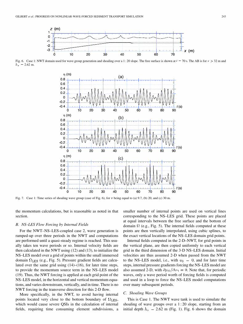
Fig. 8. Case 2: Time series of the horizontal and vertical velocity plotted for the NWT and NS–LES simulations, for the first period of run time, at the samelocation in the upper left corner of the NS–LES grid (x = 11.7 m and z = �0.63 m in Fig. 4). The x-axis: time (s).

geometry used for this case. Table I gives general data and pa-rameters. The AB is specified for 32 m.

The wavemaker law used for boundary condition (8) for thiscase is specified as the superposition of two periodic motions ofthe same amplitude, as , with0.27 m and 2.13 rad/s and 2.44 rad/s. This motionis ramped-up over three mean periods based on a law.

Fig. 6 shows the free surface computed at 70 s. We seethat wave asymmetry and steepness increase as the wave groupshoals up the slope, and one wave is close to overturning at31 m. Fig. 7 shows time series of surface elevations for threegages located at 9.7, 20, and 30 m. Early in the shoaling, at

9.7 m [Fig. 7(a)], the wave groups are already asymmetric,trough to crest, due to incident wave nonlinearity, with min-imum troughs of 0.33 m and maximum crests of 0.45 m. Non-linearity and asymmetry of the wave shape further increase for

20 and 30 m [Fig. 7(b) and (c)], with additional front-to-rearasymmetry at the top of the slope where waveheight reachesmore than 90% the local depth.

It is to be pointed out that, after an initial ramp-up lasting 10 sor so, all the time series in Fig. 7 show wave groups that recurin time with little change in amplitude, indicating that almostno reflection occurs in the NWT. This confirms that the AB/APscheme effectively absorbs incident wave energy, as can also beseen in Fig. 6, where waveheight rapidly decreases in the AB,for 32 m.

This application clearly shows the ability of the NWT to gen-erate complex, strongly nonlinear, shoaling wave climates, overan arbitrary sloping bottom.

D. Periodic Wave Flow Over a Cylindrical Obstacle

This is Case 2. Here, the dynamic pressure gradient calculatedin the NWT is used to force the NS–LES model. To verify thatthis yields realistic results for the flow in the NS–LES model,

we plotted the time series for the NWT and NS–LES models,respectively (Fig. 8), at the upper left corner of domainduring the first period of run time ( 11.7 m and 0.63 min Fig. 4). We see that velocities in both models agree reasonablywell at this time. Later in time, however, this agreement grad-ually deteriorates (results not shown here), likely for two mainreasons. First, waves generated in the NWT are not strictly pe-riodic, due to nonlinearity (e.g., Stokes drift), but in this firstillustrative application we force the NS–LES simulations by re-peating the NWT data periodically. This causes a slight phaseshift, which becomes gradually more pronounced after the ini-tial run period. Second, the magnitudes of the NS–LES sim-ulation results change as these adjust to the formation of theboundary layer over the bottom. For these reasons, the NS–LESsimulation results do not match those of the NWT exactly laterin time. However, they still produce a realistic periodic waveorbital motion.

Both detailed velocity and sediment concentration results areshown in Figs. 9 and 10, for the 11th period of run time (thefirst ten periods are model ramp-up). In this case, the suspendedsediment concentration field was initialized as a function of thebottom shear stress at the end of the tenth period.

Bedload was not computed for this initial illustration of ourcoupled model computations. For illustration purpose, we alsocaused sediment entrainment during most of the flow period, atmost locations along the bed, by adjusting upward the value of

.1) Boundary Layer Dynamics: Fig. 9(a)–(h) depicts the

boundary layer development as a series of instantaneoussnapshots of the velocity field in a streamwise-verticalplane.

Characteristic of all boundary layers, velocity profiles tend tozero along the bed, with larger near-bed velocities surroundingthe crest of the mine. This is consistent with observations that


Fig. 9. (a)–(h) Instantaneous plots of the (u; v) velocity field on the centerplane, extending roughly halfway up our numerical domain. The two vectors at the topof each plot indicate the flow direction and magnitude aloft (bottom vector) scaled relative to its maximum value (top vector), on much larger scale than the vectorsin the plots. Below: plot of the instantaneous streamwise-averaged u velocity at the top of our domain, with hash marks indicating the timing of vector plots (a)–(h).

the highest shear stresses over ripples occur either just upstream[1] or at the ripple crest [37].

Similar to the findings of [2] for a uniform oscillatory flowover sinusoidal ripples, shear layers form in the lee of the mineduring wave phases where the velocity tapers off from its max-imum value [Fig. 9(a), (b), and (e)–(g)]. However, the boundarylayer development for waves over a 75% buried cylindrical minediffers significantly from that observed in [2], where an oscilla-tory flow was forced over sinusoidal ripples. It is thought thatthe main differences are due to the phasing and spatial distri-bution of the wave forcing provided by the NWT, as compared

to a purely time-dependent oscillatory flow. This is further dis-cussed later.

As the velocity tapers off from its maximum value[Fig. 9(a)–(c) and (e)–(g)], a shear layer first forms on thelee side of the mine [Fig. 9(a), (b), (e), and (f)], as would beexpected for a typical oscillatory flow case. As the flow slowsenough so that it is about half its maximum value, some of thenear-bed velocities reverse [Fig. 9(c) and (g)] and form whatlooks to be the beginning of a typical lee vortex. However, asthe flow slows to zero [Fig. 9(d) and (h)], the pressure gradientdistribution on the mine from the NWT acts to intensify the


Fig. 10. (a) and (b) Instantaneous plots of sediment concentration contours superimposed on the (u; v), velocity field on the centerplane, extending roughly athird of the way up the numerical domain. The two vectors at the top of each plot indicate the flow direction and magnitude aloft (bottom vector), scaled relativeto its maximum value (top vector), on much larger scale than the vectors in the plots. Here, (a) corresponds to Fig. 9(g) and (b) to Fig. 9(h).

flow in the direction down the slope, contrary to the behaviorobserved in previous simulations of an oscillatory flow overripples [2].

This jet of fluid is now moving in the direction opposite tothe new flow direction. After the flow switches direction, thisnear-bed jet of fluid, which opposes the new main flow direc-tion, rolls up into a spanwise vortex on the stoss side of the mine[Fig. 9(c) and (g)]. Clearly, the vortex which forms in Fig. 9(g) ismuch larger and better defined than that in Fig. 9(c). This maybe attributed to the asymmetry of the wave (e.g., Fig. 2), be-cause the magnitude of the flow in the “positive” (left to right)direction is considerably weaker than that in the “negative” di-rection, and, therefore, less capable of destroying the stoss-sidevortex/shear layer.

2) Sediment Transport Patterns: As found in [2], the sed-iment transport patterns follow the flow field very closely.However, the entrainment patterns differ significantly becausethe boundary condition along the mine enforces the condition

. Strictly, this is only a first approximation to the correctboundary condition, which would allow for deposition andsubsequent pickup on the obstacle boundary , as the fluxcondition of [38, eq. (2)]. For the case studied here, this approx-imate boundary condition may have contributed to oscillationsin the concentration profiles which eventually lead to unrealisticbehavior in the sediment concentration field, so that the resultspresented in this section are taken from the first period after thesediment concentration was initialized. This poor behavior ofthe boundary condition (applied along the mine) was not

expected, since it produced physically reasonable results for apure-oscillatory case over the mine. We show results during thesecond half of the 11th flow period, when the flow has had achance to lose some of the influence of the initial conditions.

In general, sediment is picked up where the shear stresses aregreater than critical along the flat bottom regions both upstreamand downstream of the mine. It is then oscillated back and forthover the mine due to the action of the flow aloft. This behaviorwould be rather straightforward if it were not for the formationof vortices on the stoss slope of the mine during every half-pe-riod. As in the case of vortex ripples [37], the stoss vortex acts totrap any sediment aloft. Because this vortex forms while the hor-izontal velocity is large, most of the sediment upstream of themine (in much lower concentrations) is swept past the vortexduring its lifetime, and is trapped there. This process is visual-ized in Fig. 10. Fig. 10(a) shows the stoss vortex long after itsformation, after it has trapped a significant amount of sediment.This sediment trapping may be enhanced by the slightly down-ward velocity aloft due to the wave coupled with the blocking bythe mine. Fig. 10(b) shows that, as the velocity turns around, thispuff of sediment is then starting to be swept out of the domain.

IV. CONCLUSION

The coupling between the NWT and the NS–LES modelto simulate wave-induced sediment transport has producedinteresting boundary layer dynamics under a realistic orbitalwave motion. The main conclusions to be drawn include thefollowing.


• The approach employed here successfully produces a non-linear orbital wave-like flow in the NS–LES simulationsfor periodic waves.

• The boundary layer motions around the partially buriedcylindrical obstacle representing a mine, differ consider-ably between the wave and pure oscillatory flow cases, andas well with those which typically form around ripples inoscillatory flows, as in [2]. The major difference here isthat a spanwise vortex forms on the stoss slope of the mineevery half period, whereas a spanwise vortex would nor-mally form in the lee of the mine (or ripple) in a pure os-cillatory flow case.

• The sediment transport dynamics are very similar to pre-vious simulations with the NS–LES model [1], [2] in thatthey are heavily guided by the boundary layer motions.Of particular interest, we find that the stoss vortex, whichforms every half cycle, acts to trap previously entrainedsediment, which flows past it, as the velocity tapers offfrom its maximum value (cf., [30], which deals with trans-port over ripples in oscillatory flow and whose entrainmentpatterns are quite similar to those observed here, albeit withsomewhat different timing due to the effect of the obstacle).

The coupled simulations with the NWT, NS–LES, and sed-iment transport models reported here were only done for a flatbottom with the partially buried obstacle. Cases with a slopingbathymetry are still being worked on, particularly with respectto the NS–LES model convergence, which is slower in suchcases, likely due to stronger wave nonlinearity.

The computations of shoaling wave groups illustrate the capa-bilities of the NWT to simulate the development of irregular andhighly nonlinear waveforms, such as occurs for ocean swells.Cases of sediment transport over a sloping bottom, forced bysuch complex shoaling wave fields will be reported in futurework.

Finally, we can think of four model elements that could beadded in the future to our coupled model system, namely: 1) im-plementation of a log-law boundary condition in the momentumequation [36]; 2) a flux boundary condition for suspended sed-iment transport at the bed, as discussed earlier; 3) a bedloadmodule; and 4) an algorithm to allow dynamic movement of thebed as a function of time (n.b., the current simulations have afixed bed form). The last algorithm would allow simulation ofwave-induced ripple formation and migration [5], or scouring/burial near-bottom obstacles [6], [10]. Our modeling approachaffords this capability and the addition of a moving bottom isongoing work that will also be reported in future papers.

ACKNOWLEDGMENT

The authors would like to thank the U.S. Department of De-fense (DOD) High Performance Computing Modernization Pro-gram for providing a grant of computer time and the anonymousreviewers for the cogent and perceptive comments.

REFERENCES

[1] E. A. Zedler and R. L. Street, “Large-eddy simulation of sedimenttransport: Currents over ripples,” J. Hydraulic Eng., vol. 127, no. 6,pp. 444–452, 2001.

[2] E. A. Zedler and R. L. Street, “Nearshore sediment transport processes:Unearthed by large-eddy simulation,” in Proc. 28th Int. Conf. Coast.Eng., J. M. Smith, Ed., 2002, pp. 2416–2504.

[3] B. Barr, D. Slinn, T. Pierro, and K. Winters, “Modeling unsteady tur-bulent flows over ripples: Reynolds-averaged Navier-Stokes equations(RANS) versus large-eddy simulation (LES),” J. Geophys. Res., vol.109, no. C09009, pp. 1–19, 2004.

[4] Y. Chang and A. Scotti, “Numerical simulation of turbulent, oscillatoryflow over sand ripples,” J. Geophys. Res., vol. 109, no. C09012, pp.1–16, 1991.

[5] S. I. Voropayev, G. B. McEachern, D. L. Boyer, and H. J. S. Fernando,“Dynamics of sand ripples and burial/scouring of cobbles in oscillatoryflow,” Appl. Ocean Res., vol. 21, no. 5, pp. 249–261, 1999.

[6] S. I. Voropayev, F. Y. Testik, H. J. S. Fernando, and D. L. Boyer,“Burial and scour around short cylinder under progressive shoalingwaves,” Ocean Eng., vol. 30, no. 13, pp. 1647–1667, 2003.

[7] S. T. Grilli and J. Horrillo, “Shoaling of periodic waves over barred-beaches in a fully nonlinear numerical wave tank,” Int. J. Offshore PolarEng., vol. 9, no. 4, pp. 257–263, Dec. 1999.

[8] S. T. Grilli, S. Voropayev, F. Y. Testik, and H. J. S. Fernando, “Numer-ical modeling and experiments of wave shoaling over buried cylindersin sandy bottom,” in Proc. 13th Offshore Polar Eng. Conf., Honolulu,HI, 2003, pp. 405–412.

[9] S. T. Grilli, S. Voropayev, F. Y. Testik, and H. J. S. Fernando, “Numer-ical modeling and experiments of periodic waves shoaling over semi-buried cylinders in sandy bottom,” J. Waterways Port Coast. OceanEng., 2007, submitted for publication.

[10] S. I. Voropayev, F. Y. Testik, H. J. S. Fernando, and D. L. Boyer, “Mor-phodynamics and cobbles behavior in and near the surf zone,” OceanEng., vol. 30, no. 14, pp. 1741–1764, 2003.

[11] S. T. Grilli, J. Skourup, and I. A. Svendsen, “An efficient boundaryelement method for nonlinear water waves,” Eng. Anal. Boundary El-ements, vol. 6, no. 2, pp. 97–107, 1989.

[12] S. T. Grilli and I. A. Svendsen, “Corner problems and global accuracyin the boundary element solution of non-linear wave flows,” Eng. Anal.Boundary Elements, vol. 7, no. 4, pp. 178–195, 1990.

[13] S. T. Grilli and R. Subramanya, “Numerical modeling of wave breakinginduced by fixed or moving boundaries,” Comput. Mech., vol. 17, pp.374–391, 1996.

[14] S. T. Grilli and J. Horrillo, “Numerical generation and absorption offully nonlinear periodic waves,” J. Eng. Mech., vol. 123, no. 10, pp.1060–1069, 1997.

[15] S. T. Grilli, R. Subramanya, I. A. Svendsen, and J. Veeramony,“Shoaling of solitary waves on plane beaches,” J. Waterway PortCoast. Ocean Eng., vol. 120, no. 6, pp. 609–628, 1994.

[16] S. T. Grilli and J. Horrillo, “Fully nonlinear properties of periodicwaves shoaling over slopes,” in Proc. 25th Int. Conf. Coast. Eng., Or-lando, FL, Sep. 1996, pp. 717–730.

[17] S. T. Grilli, I. A. Svendsen, and R. Subramanya, “Breaking criterionand characteristics for solitary waves on slopes,” J. Waterway PortCoast. Ocean Eng., vol. 123, no. 3, pp. 102–112, 1997.

[18] S. Guignard, S. T. Grilli, R. Marcer, and V. Rey, “Computation ofshoaling and breaking waves in nearshore areas by the coupling ofBEM and VOF methods,” in Proc. 9th Offshore Polar Eng. Conf., Brest,France, May 1999, vol. III, pp. 304–309.

[19] C. Lachaume, B. Biausser, S. T. Grilli, P. Fraunie, and S. Guignard,“Modeling of breaking and post-breaking waves on slopes by couplingof BEM and VOF methods,” in Proc. 13th Offshore Polar Eng. Conf.,Honolulu, HI, May 2003, pp. 353–359.

[20] B. Biausser, S. T. Grilli, and P. Fraunie, “Numerical simulations ofthree-dimensional wave breaking by coupling of a VOF method and aboundary element method,” in Proc. 13th Offshore Polar Eng. Conf.,Honolulu, HI, May 2003, pp. 333–339.

[21] B. Biausser, S. T. Grilli, P. Fraunie, and R. Marcer, “Numericalanalysis of the internal kinematics and dynamics of three-dimensionalbreaking waves on slopes,” Int. J. Offshore Polar Eng., vol. 14, no. 4,pp. 247–256, 2004.

[22] Y. Zang, R. L. Street, and J. R. Koseff, “A dynamic mixed subgrid-scale model and its application to turbulent recirculating-flows,” Phys.Fluids, vol. 5, no. 12, pp. 3186–3196, 1993.

[23] L. C. vanRijn, “Sediment transport 1. Bed-load transport,” J. HydraulicEng., vol. 110, no. 10, pp. 1431–1456, 1984.

[24] A. Nakayama, H. Noda, and K. Maeda, “Similarity of instantaneousand filtered velocity fields in the near wall region of zero-pressure gra-dient boundary layer,” Fluid Dyn. Res., vol. 35, pp. 299–321, 2004.

[25] A. Nakayama, Personal communication. 2005.


[26] L. C. vanRijn, Principles of Sediment Transport in Rivers, Estuariesand Coastal Seas. Amsterdam, The Netherlands: Aqua, 1993.

[27] L. C. vanRijn, “Sediment transport 3. Bed forms and alluvial rough-ness,” J. Hydraulic Eng., vol. 110, no. 12, pp. 1733–1754, 1984.

[28] M. Garcia and G. Parker, “Entrainment of bed sediment into suspen-sion,” J. Hydraulic Eng., vol. 117, no. 4, pp. 414–435, 1991.

[29] D. M. Admiraal, M. H. Garcia, and J. F. Rodriquez, “Entrainment re-sponse of bed sediment to time-varying flows,” Water Resources Res.,vol. 36, no. 1, pp. 335–348, 2000.

[30] E. A. Zedler and R. L. Street, “Sediment transport over ripples in an os-cillatory flow,” J. Hydraulic Eng., vol. 132, no. 22, pp. 180–193, 2006.

[31] S. T. Grilli and R. Subramanya, “Quasi-singular integrations in themodelling of nonlinear water waves,” Eng. Anal. Boundary Elements,vol. 13, no. 2, pp. 181–191, 1994.

[32] B. P. Leonard, “A stable and accurate convective modelling procedurebased on quadratic upstream interpolation,” Comput. Methods Appl.Mech. Eng., vol. 19, no. 1, pp. 59–98, 1979.

[33] B. P. Leonard, “Simple high accuracy resolution program for convec-tive modeling of discontinuities,” Int. J. Numer. Meth. Fluids, vol. 8,pp. 1291–1318, 1988.

[34] Y. Zang, R. L. Street, and J. R. Koseff, “A non-staggered grid, frac-tional step method for time-dependent incompressible Navier Stokesequations in curvilinear coordinates,” J. Comput. Phys., vol. 114, no.1, pp. 18–33, 1994.

[35] Y. H. Tseng and J. H. Ferziger, “A ghost-cell immersed boundarymethod for flow in complex geometry,” J. Comput. Phys., vol. 192, no.2, pp. 593–623, Dec. 2003.

[36] I. Senocak, A. S. Ackerman, D. E. Stevens, and N. N. Mansour, “To-pography modeling in atmospheric flows using the immersed boundarymethod,” Center Turbulence Res., NASA, Stanford, CA, Annual Res.Briefs, 2004.

[37] J. F. A. Sleath, “The suspension of sand by waves,” J. Hydraulic Res.,vol. 20, no. 5, pp. 439–452, 1982.

[38] I. Celik and W. Rodi, “Suspended sediment transport capacity for openchannel flows,” J. Hydraulic Eng., vol. 128, no. 12, pp. 1051–1059,1991.

Richard W. Gilbert received the B.S. degree in civilengineering from the University of Arizona, Tempe,and the M.S. degree in ocean engineering from theUniversity of Rhode Island, Narragansett, in oceanengineering in spring 2006.

He practiced structural engineering for a fewyears and obtained his license as a professional engi-neer. Currently, he works for McLaren EngineeringGroup, West Nyack, NY, designing coastal structuresand performing coastal modeling throughout NewEngland. Study areas include current and wave mod-

eling within harbors, and coastal erosion hazard area mapping and mitigationdesign.

Emily A. Zedler received the B.S. degree inmathematics from the University of California atDavis, and the M.S. degree from the University ofCalifornia at Berkeley, and the Ph.D. degree from theStanford University, Palo Alto, CA, in environmentalengineering. Her Ph.D. and postdoctoral studies atStanford University focused on LES of sedimenttransport over rippled bedforms.

She works at the Santa Clara Valley Water District,San Jose, CA, where she applies her background inenvironmental engineering to tackle real-world flood

control problems. Her work at the District includes open channel flow modelingand sediment transport analysis towards the design of improved capacity andstable channels.

Stéphan T. Grilli received the M.S. and Ph.D. de-grees from the University of Liège, Liège, Belgium.

He moved to the United States in 1987. He spentthree years as a member of research faculty at theUniversity of Delaware, Newark, before he joinedthe faculty of the University of Rhode Island, Nar-ragansett, in 1991, where he is now a DistinguishedEngineering Professor and Chair of the Departmentof Ocean Engineering. He studies ocean waves,tsunamis, and related fluid mechanics and marinehydrodynamics problems. Although he conducted

experimental work, his research focuses on the numerical modeling of complexnonlinear wave flows, such as wave breaking, extreme wave effects on oceanstructures, and wave-induced sediment motion in coastal regions. He alsostudies waves induced by underwater landslides.

Robert L. Street received the M.S. and Ph.D. de-grees from the Stanford University, Palo Alto, CA.

He joined the faculty at Stanford University in1962. He is the William Alden and Martha CampbellProfessor [Emeritus] in the School of Engineeringand Emeritus Professor of Fluid Mechanics andApplied Mathematics in the Department of Civil andEnvironmental Engineering. He studies geophysicalfluid motions. His research focuses on the modelingof turbulence in fluid flows, which are often strat-ified, and includes numerical simulation of coastal

upwelling, internal waves and sediment transport in coastal regions, flow inrivers and estuaries, and valley winds in the atmosphere.

Date post:	07-May-2018
Category:	Documents
Upload:	nguyenkhanh
View:	215 times
Download:	1 times

236 IEEE JOURNAL OF OCEANIC ENGINEERING, … Coastal Geosciences Division Mine Burial Burial Program...

Documents