PERFORMANCE OF THE FIRST QDDD SPECTROGRAPH

M. Goldschmidt, D. Rieck and C.A. WiednerMax-Planck-Institut fur Kernphysik, Heidelberg, Germany

Abstract

A new type of magnetic spectrograph for pre­cision spectroscopy of charged particles fromnuclear reaction has been put into operation. Thisspectrograph consists of a quadrupole followedby three dipoles, a multipole element and an elec­trostatic deflector. The ion optical lay-outfeatures a point to point image in both planesand in addition an axial intermediate image. Thecomponents of the system have been mapped. Afterassembling the spectrograph has been ray tracedwith 3He particles of 24 MeV. The resolvingpower at tae full solid angle of 13 msr isdp/p ~ 10- for several reactions investigatedso far.

~--_......--~

1m

I. Introduction

Present problems in low energy nuclear spec­troscopy require magnetic spectrographs withhigh solid angle and a resolving power of p/dp104 i.e. comparable to the energy stability oftandem accelerators or single-turn extractioncyclotrons. The detection of particles in thefocal plane should be accomplished with positionsensitive detectors - e.g. multiwire proportionalchambers - to have on-line control of the measure­ments. Since the interest in nuclear reactionswith heavy particles is steadily increasing meansfor correcting the kinematic broadening have tobe provided.

QDDD SPECTROGRAPH

T - Target chamberQ. - QuadrupoleD1-D

3- Dipoles

ME - MUltipole elementED - Electrost. DeflectorFE - Focal planeD - Detector chamber

Fig. 1. Plan view of the spectrograph. With outermost particle trajectoriesand beam envelope of central momentum.

100

In detail the following specifications havebeen required for the spectrograph:a) Solid angle n = 13 msrb) Resolving power p/dp = 104

at the full solid anglec) Momentum range: 80 MeV/c to 500 MeV/cd) Simultaneously accepted momentum bite op/p=10%e) Dispersion D = 20 cm/% momentum bite along

the focal planef) D/M = 10gA Provision of a multipole element for kine­

matic correction up to dp/(p.d9) = 0.3/rad.

The high dispersion specified is necessaryto obtain the desired resolution with on-linedetectors having a spatial resolution of about1 mm.

The criteria mentioned can be met by thenew type spectrographs of the QDDD type, i.e.systems containing a quadrupole and three di-

poles. These feature in addition to doublefocussing an intermediate axial image between thefirst and second dipole magnet. The method ofdesigning intermediate image spectrographs usingnumerical raY1tracing has been described by Engeand Kowalski. Their paper also contains thedetails of the ion optical layout of the QDDDspectrograph, which is shown in Fig.1. To correctfor aberrations curvatures up to fifth order onthe pole faces had to be provided. The coeffi­cients of these curvatures will be compared tothose measured in paragrap~ III. Before the re­sults of ray tracing with He particles of24 MeV are discussed in IV, section II, dealswith some of the technological aspects.

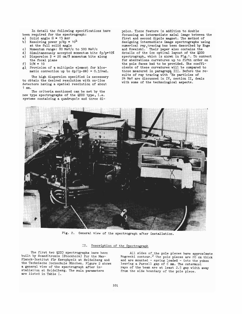
Fig. 2. General view of the spectrograph after installation.

II. Description of the Spectrograph

The first two QDDD spectrographs have beenbuilt by Scanditronix (Stockholm) for the Max­Planck-Institut fur Kernphysik at Heidelberg andthe Technische Hochschule Munchen. Figure 2 showsa general view of the spectrograph after in­stallation at Heidelberg. The main parametersare listed in Table I.

101

All sides of the pole pieces have approximateRogowski contour. 2 The pole pieces are 20 cm thickand are mounted - spring loaded - into the yokesleaving a Purcell gap of 6 mm. The outermostrays of the beam are at least 2.5 gap width awayfrom the side boundary of the pole piece.

TABLE II. Mechanical Displacements Correspondingto one Bin Width

Aperture of Quadrupole d 12 cm Entrance

Horizontal AcceptanceSecond Dipole

Exit8 2:. 55 mrd

Vertical Acceptance C/J 2:. 63 mrd Third Dipole EntranceExit

TABLE I. Technical Specifications

Bending Radius 95 cm ~ p ; 105 cm

Magnetic Field 2.7 kG ; B; 17 kG

Total Angle of Deflection ¢=1800

Magnet Type H-Magnets

Quadrupole Danby Figure-of-Eight

Magnet Pole Gap d = 8 cm

SystemComponent

Quadrupole

First Dipole

Pole Face

Entran<::eExit

EntranceExit

D(mm)

2.331.00

0.600.35

0.300.34

0.901. 10

ROA PVA(deg. ) (deg. )

0.50 not calc.

1. 10 0.05

1. 46 0.11

1.82 0.46

Length of Focal Plane L 2.20 m0< < 0

Angular Range -15 =8S =+ 155

Power Required for Max. Field 330 kW

Weight Including Support 140 tons

D - Displacement along the beam axis; ROA ­Rotation about optical axis; RVA-Rotation aboutvertical axis

The pole boundaries facing the beam are milledwith a computer-controlled contour cutter. It hadbeen helpful for both, the check of the accuracyof the mechnical tolerances and the alignmentand adjustment of the components with respectto each other that immediately after the millingprocedure small holes were drilled into the polepieces. For the Hall probe measurements of thefringe fields needles fitted snug into the holes.The strong nonuniformity of these was measuredin the coordinate system of the field mappingmachine taken on both faces of the pole pieceand the data hence could be transformed to onecoordinate system.

Tolerances

In order to obtain numerical values for thetolerances to be specified for the manufacturerfirst order calculations with the computer pro-'gram TRANSPORT have been made. 3 In each run oneof the system components was shifted or turnedwith respect to the others and by normal matrixmultiplication technique the beam trajectory wascalculated through the system.

The quotient of aispersion D = 20 cm/% and re­solving power R = 10 specifies one resolutionbin width, which corresponds to 2 mm. The mecha­nical displacements corresponding to one binwidth for the QDDD spectrograph are summarizedin Table II.

Attached to the magnets are field clampspreceding each pole piece boundary. By movingoff these the effective field boundary can beshifted to a certain extent, remachining themcould be used to correct for deviations from thedesigned shape of the pole boundary.

Material Properties and Results of Machining

The material used for the pole plates isforged steel with the following chemicalanalysis: 5

C(%) Si (%) Mn(%) p(%) S(%) N(%)

0.02 0.22 0.40 0.02 0.013 0.009

B(T)

2.

Q3DMAGNETISING CURVE

PROBE 6

0.5

300

30H (A/em)

o

0l--------l.-------I...---....l...----1200

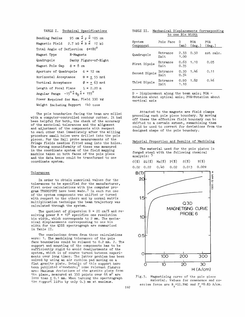
Fig.3. Magnetising curve of the pole piecematerial. Values for remanence and co­

ercive force are B =11.9kG and F =0.85 A/em.r c102

The conclusions drawn from these calculationswere: 1. The machining tolerances of the poleface boundaries could be relaxed to 0.2 mm. 2. Thesupport and mounting of the components has to besufficiently rigid to avoid deadjustments of thesystem, which is of course turned between experi­ments over long times. The latter problem has beensolved by using an air cushion pad moving on aflat gran~te plate. Detaius of this support havebeen publlshed elsewhere; some relevant fi~res

are: IlJaximum deviat ions of the grani te plate fromthe plane, measured at 350 points over 66 m2 areless than 2:. 0.1 mm. vfuen turning the spectrographthe support lifts by only 0.3 mm at maximum.

Magnetising curves on this material have beenmade; a typical example is shown in Fig. 3 .

Detailed mappings of the mechanical tole­rances revealed deviations from the designed poleshapes of less than 0.2 rom. The gap width of themagnets differed by not more than ~ 0.005 rom fromthe expected 80 rom measured in a grid of 5 cmbase length. To accomplish this, pole pieces havebeen partly handscraped after the final machining.

III. Field Mapping

Before assembly the components of the spec­trograph have been mapped at various excitations.The excitation procedure was crucial for the uni­formity and reproducibility of the field distri­bution, which is dealt with in another paper ofthis conference. 6 The homogeneous parts of thedipole magnets have been mapped with NMR probes,fringe fields and quadrupole by Hall probe measu­rements.

Homogeneous Parts of Dipoles

The excitation procedure yielding best uni­formity was found to be the following. First themagnet is excitedto 17 kG; with a speed of80 G/sec the field is run down and the desiredfield "undershot" by 20% of the final setting,which is then approached at a rate of 40 G/sec.Figure 4 shows a typical field map of dipole 1.NMR - probe measurements were taken in a grid ofapp. 5 cm x 5 cm. The deviation from the averagefield level is shown cross-hatched for measure­ments across the magnet. Essentially the same re­sults have been achieved for fields between 3and 15 kG and also for dipole 2. The maximumdeviation in a region 2.5 gap width away fromthe pole boundariee in no case exceededdB/B =~ 1.5 x 10-

Q30 SPECTROGRAPH 01

B· 9,16 kG

I! 10-4

¥: '63'10-5

'Fig. 4. Typical field map of dipole 1

Fig. 5. Fringe field fall-off along different cuts at exit dipole

g.. o mm

B·6KG.. 100 mmx, z 400mm,.." 260 mm

B" 3 KG . )(" 260 mm8.15KG x" 260 mm

8 Z[cm]

Q3D SPECTROGRAPHFRINGE FIELD FALL OFFEXIT 01NORM. AT EFB

o

EFB

-2-4-6-8-10

1.0

01

103

Fringe Fields

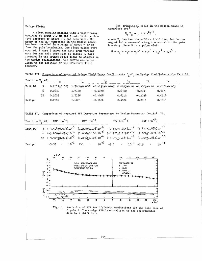
A field mapping machine with a positioningaccuracy of about 0.2 mm and a Hall probe with atest accuracy of about 2 G has been used. Thedecay of the ~r- component in the median planehas been measufed in a range of about + 30 cmfrom the pole boundaries. The field ci~ps weremounted. Figure 5 shows the data from variouscuts for the exit pole face of dipole 1. Alsoincluded is the fringe field decay as assumed inthe design calculations. The curves are norma­lised to the position of the effective fieldboundary.

The frin~ing By field in the median plane isdescribed by:

B IB = ( 1 + eS)-1,y 0

where Bo denotes the uniform field deep inside themagnet and s measured along the normal to the poleboundary. Here S is a polynomial:

2 3 4 5S = Co + c1s + c2s + c

3s + c4s + c

5s .

TABLE III. Comparison of Measured Fringe Field Decay Coefficients Co-C5 ~t~o~D~e~s~ig~n~C~o~e~f~f~i~c~i~e~n~t~s~f~or~E=x~~~'t~D~2~.

Position B (kG) c c1 c2 c3 c4 c

50 0

Exit D2 3 0.2612!-0.003 1. 7080!-0. 008 -0. 4132!-0. 0165 0.6295!-0.01 -0.2009.:t.0.01 0.0172.:t.0 •003

6 0.2639 1.7150 -0.4170 0.6300 -0.2043 0.0179

12 0.2622 1. 7176 -0.4098 0.6312 -0.2038 0.0118

Design 0.2049 1. 6821 -0.5654 0.4004 0.0011 0.1663

TABLE IV. Comparison of Measured EFB Curvature Parameters to Design Parameter for Exit D2.

RAP (cm-1 ) CAT (cm-3 ) -4 CNN (cm-5 )Position Bo(kG) CFV (cm )

Exit D2 3 (-3.504+0.074)10-3 (1.228+0.108)10-6 (2. 552.:t.7.195)10-9 (6. 447.:t.1. 884)10-10

6 (-3.400:0.074)10-3 (1.688:0.108)10-6 (-6. 720.:t.7.189)10-9 (2.026.:t.1.883)10-10

12 (-3.397~0.074)10-3 (1.836~0.108)10-6 (-5.972.:t.7.187)10-9 (1. 229.:t.1. 883)10-10

Design -3.37 10-3 2.1 10-6-9.7 10-9 -2.5 10-11

ENTRANCE 02• 3kGo 6kG~ 12kG-CALC.

a 3 0 SPECTROGRAPHVARIATION OF EFB FORDIFFERENT FIELDS

12 .....-~~--:-:;:...--~=------=;:...----.:.::.......-..:;:..---:;:...----T---.;:.-----;.:~-...,:----.,.:....---....,

10

8

6

'? 4

~ 2

o-2

-4 L---L__.L-_---L__....I..-_---l__....L__l....-_....J....__.L-_........J..__...L...._---J~_....L.....J

-25x [em]

-20-15-10-5o510

l:~~_..Ic:~:::::::_3k_1...1..2k_G_6k_G---l.__....L.._ L___.L...__.....J...__.J.__ ___L._=======__'_____l LI__::s~J35 30 25 20 15

Fig. 6. Variation of EFB for different excitations for the pole face ofdipole 2. The design EFB is normalized to the experimentaldata by a shift in z.

lOt"

60

~.

3003060r[mmJ

IZMI~4em

J=1778A

9=1.2 kGauss/em

30 0 30r [mmJ

~.~

.~

J =885.0 A 19 =0.6 kGauss/em .1

.1.~

.1:/

"".~

,Ix

~

\ I ZMI ~ 4 em;~

~··l".\".\:.\'g,:,,::-:

60

.......---------------, :rii:~

.......---------------, :ra:~

20

4.0

-20

-4.0

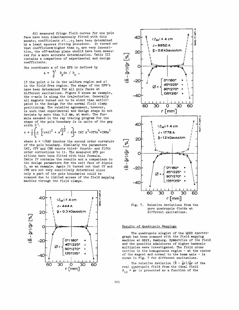
Fig. 7. Relative deviations from thepure quadrupole fields atdifferent excitations.

4.0

rJ 20~

UL

10) 0-L10)

1

lID -20--4.0

II~o

L...JL

10)--L10)

I

ICO

Results of Quadrupole Mappings

The quadrupole singlet of the QDDD spectro­graph has been scanned with the field mappingmachine at DESY, Hamburg. Symmetries of the fieldand the possible admixtures of higher harmonicmultipoles were investigated. The field crosssection in the homogeneous region - at the centerof the magnet and normal to the beam axis - isshown in Fig. 7 for different excitations.

The relative deviation (B - gr)/gr of thereal quadrupole field from the ideal fieldBid = gr is presented as a function of the

40IZMI~4em

J = 444 A

20 9 = 0.3 kGauss/emrI~

~L

101 0-L101

I

HD -20 rO/1800 •45°/225. 0

0= 90°/270° x

135°/315°

All measured fringe field curves for one poleface have been simultaneously fitted with thisansatz; coefficients c1 ••• c5 have been determinedby a least squares fitting procedure. It turned outthat coefficien$higher than c3 are very insensi­tive, the off-median plane should have been measu­red for a more accurate determination. Table IIIcontains a comparison of experimental and designcoefficients.

The coordinate a of the EFB is defined by

a = SJ1 B ds / B ,o Y 0

if the point 0 is in the uniform region and s1in the field free region. The shape of the EFB'shave been determined for all pole faces atdifferent excitations. Figure 6 shows an example,the z-axis is along the trajectories. Generallyall magnets turned out to be wider than antici­pated in the design for the normal field clamppositioning. The relative agreement, however,is such that experimental and design shape do notdeviate by more than 0.2 mm, at most. The for­mula assumed in the ray tracing program for theshape of the pole boundary is in units of the gapwidth D1 1

s =i(:t [cZ+A)2 + x2J2 -j+ CAT x

3+CFV}+CNNx

5

where A = 1/RAP denotes the second order curvatureof the pole boundary. Similarly the parametersCAT, CTV and CNN denote third- fourth- and fifthorder corrections to it. The measured EFB po­sitions have been fitted with this formula.Table IV contains the results and a comparison tothe design parameters for the exit face of dipole2, as an example. Again it turned out that CV andCNN are not very sensitively determined sinceonly a part of the pole boundaries could bescanned due to limited access of the field mappingmachine through the field clamps.

105

1.0x[mmJ

-20 )It m-10

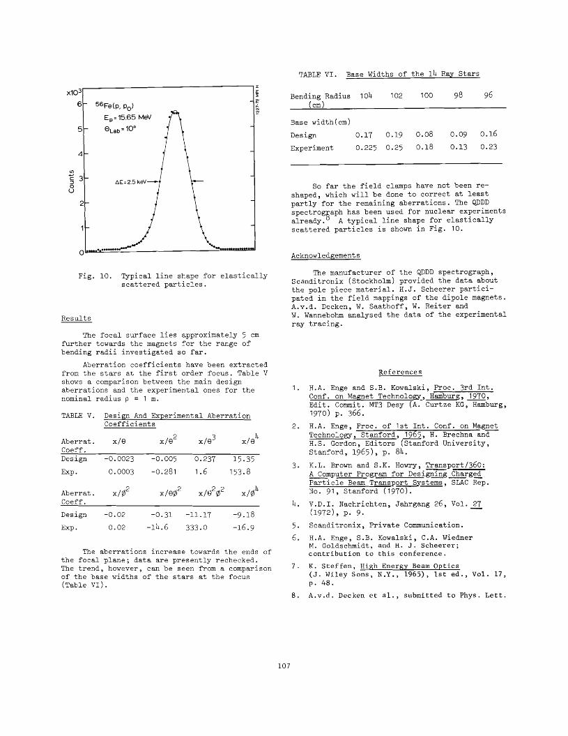
Effect of clamp displacement onEFB at exit Dl.

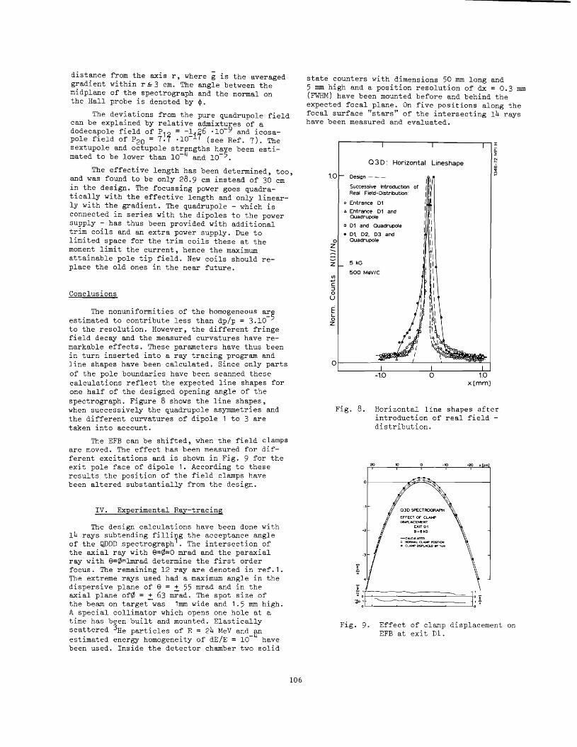
Horizontal line shapes afterintroduction of real field ­distribution.

20

Q 3 D: Horizontal Lineshape

5 kG

Design ---

Successive Introduction ofReal Field-Distribution:

o Entrance 01

"Entrance 01 andQuadrupole

o 01 and Quadrupole

• 01, 02, 03 andQuadrupole

Fig. 9.

Fig. 8.

EL.oZ

oZ

z

Ul+"C:JoU

1.0

state counters with dimensions 50 mm long and5 mm high and a position resolution of dx = 0.3 mm(FWHM) have been mounted before and behind theexpected focal plane. On five positions along thefocal surface "stars" of the intersecting 14 rayshave been measured and evaluated.

distance from the axis r, where g is the averagedgradient within r £:: 3 cm. The angle between themidplane of the spectrograph and the normal onthe Hall probe is denoted by ¢.

The deviations from the pure quadrupole fieldcan be explained by relative admixtures of adodeca~ole field of P12 = -~.26 .10-9 and icosa­pole fleld of P20 = 7.·( ·10 17 (see Ref. 7). Thesextupole and octupole strffngths have been esti­mated to be lower than 10- and 10-5•

The effective length has been determined, too,and was found to be only 28.9 cm instead of 30 cmin the design. The focussing power goes quadra­tically with the effective length and only linear­ly with the gradient. The quadrupole - which isconnected in series with the dipoles to the powersupply - has thus been provided with additionaltrim coils and an extra power supply. Due tolimited space for the trim coils these at themoment limit the current, hence the maximumattainable pole tip field. New coils should re­place the old ones in the near future.

IV. Experimental Ray-tracing

The design calculations have been done with14 rays subtending filling the acceptance angleof the QDDDspectrograph1. The intersection ofthe axial ray with e=¢=o mrad and the paraxialray with e=¢~lmrad determine the first orderfocus. The remaining 12 ray are denoted in ref.1.The extreme rays used had a maximum angle in thedispersive plane of e = ~ 55 mrad and in theaxial plane of¢ = ~ 63 mrad. The spot size ofthe beam on target was 1mm wide and 1.5 mm high.A special collimator which opens one hole at atime has been built and mounted. Elasticallysca:tered 3He particles 0: E = 24 MeV and_~nestlmated energy homogenelty of dElE = 10 havebeen used. Inside the detector chamber two solid

Conclusions

The nonuniformities of the homogeneous a~5

estimated to contribute less than dplp = 3.10to the resolution. However, the different fringefield decay and the measured curvatures have re­markable effects. These parameters have thus beenin turn inserted into a ray tracing program andline shapes have been calculated. Since only partsof the pole boundaries have been scanned thesecalculations reflect the expected line shapes forone half of the designed opening angle of thespectrograph. Figure 8 shows the line shapes,when successively the quadrupole asymmetries andthe different curvatures of dipole 1 to 3 aretaken into account.

The EFB can be shifted, when the field clampsare moved. The effect has been measured for dif­ferent excitations and is shown in Fig. 9 for theexit pole face of dipole 1. According to theseresults the position of the field clamps havebeen altered substantially from the design.

106

x103

6 56Fe(p, po)

Ep =15.65 MeV

5 6 Lab =100

4

(/)......

3c:J0u

2

Fig. 10. Typical line shape for elasticallyscattered particles.

Results

The focal surface lies approximately 5 cmfurther towards the magnets for the range ofbending radii investigated so far.

Aberration coefficients have been extractedfrom the stars at the first order focus. Table Vshows a comparison between the main designaberrations and the experimental ones for thenominal radius p = 1 m.

TABLE V. Design And Experimental AberrationCoefficients

Aberrat. x/e x/e2

x/e3 x/e4

Coeff.Design -0.0023 -0.005 0.237 15.35

Exp. 0.0003 -0.281 1.6 153.8

Aberrat. x/(!p x/e(/J2 x/fi(/J2 x/(/J4Coeff.

Design -0.02 -0.31 -11.17 -9.18

Exp. 0.02 -14.6 333.0 -16.9

The aberrations increase towards the ends ofthe focal plane; data are presently rechecked.The trend, however, can be seen from a comparisonof the base widths of the stars at the focus(Table VI).

TABLE VI. Base Widths of the 14 Ray Stars

Bending Radius 104 102 100 98 96(cm)

Base width(cm)

Design 0.17 0.19 0.08 0.09 0.16

Experiment 0.225 0.25 0.18 0.13 0.23

So far the field clamps have not been re­shaped, which will be done to correct at leastpartly for the remaining aberrations. The QDDDspectrogBaph has been used for nuclear experimentsalready. A typical line shape for elasticallyscattered particles is shown in Fig. 10.

Acknowledgements

The manufacturer of the QDDD spectrograph,Scanditronix (Stockholm) provided the data aboutthe pole piece material. H.J. Scheerer partici­pated in the field mappings of the dipole magnets.A.v.d. Decken, W. Saathoff, W. Reiter andW. Wannebohm analysed the data of the experimentalray tracing.

References

1. H.A. Enge and S.B. Kowalski, Proc. 3rd Int.Conf. on Magnet Technology_, Hamburg, 1970,Edit. Commit. MT3 Desy (A. Curtze KG, Hamburg,1970) p. 366.

2. H.A. Enge, Proc. of 1st Int. Conf. on MagnetTechnology, Stanford, 1965, H. Brechna an~H.S. Gordon, Editors (Stanford University,Stanford, 1965), p. 84.

3. K.L. Brown and S.K. Howry, Transport/360:A Computer Program for Designing Charg~

Particle Beam Transport Systems, SLAC Rep.No. 91, Stanford (1970).

4. V.D.I. Nachrichten, Jahrgang 26, Vol. 27(1972), p. 9. -

5. Scanditronix, Private Communication.

6. H.A. Enge, S.B. Kowalski, C.A. WiednerM. Goldschmidt, and H. J. Scheerer;contribution to this conference.

7. K. Steffen, High Energy Beam Optics(J. Wiley Sons, N.Y., 1965), 1st ed., Vol. 17,p. 48.

8. A.v.d. Decken et al., submitted to Phys. Lett.

107