260 IEEE TRANSACTIONS ON PATTERN ANALYSIS AND …€¦ · Geometric Mean for Subspace Selection...

Geometric Mean for Subspace SelectionDacheng Tao, Member, IEEE, Xuelong Li, Senior Member, IEEE, Xindong Wu, Senior Member, IEEE,

and Stephen J. Maybank, Senior Member, IEEE

Abstract—Subspace selection approaches are powerful tools in pattern classification and data visualization. One of the most

important subspace approaches is the linear dimensionality reduction step in the Fisher’s linear discriminant analysis (FLDA), which

has been successfully employed in many fields such as biometrics, bioinformatics, and multimedia information management. However,

the linear dimensionality reduction step in FLDA has a critical drawback: for a classification task with c classes, if the dimension of the

projected subspace is strictly lower than c� 1, the projection to a subspace tends to merge those classes, which are close together in

the original feature space. If separate classes are sampled from Gaussian distributions, all with identical covariance matrices, then the

linear dimensionality reduction step in FLDA maximizes the mean value of the Kullback-Leibler (KL) divergences between different

classes. Based on this viewpoint, the geometric mean for subspace selection is studied in this paper. Three criteria are analyzed:

1) maximization of the geometric mean of the KL divergences, 2) maximization of the geometric mean of the normalized KL

divergences, and 3) the combination of 1 and 2. Preliminary experimental results based on synthetic data, UCI Machine Learning

Repository, and handwriting digits show that the third criterion is a potential discriminative subspace selection method, which

significantly reduces the class separation problem in comparing with the linear dimensionality reduction step in FLDA and its several

representative extensions.

Index Terms—Arithmetic mean, Fisher’s linear discriminant analysis (FLDA), geometric mean, Kullback-Leibler (KL) divergence,

machine learning, subspace selection (or dimensionality reduction), visualization.

Ç

1 INTRODUCTION

FISHER’S linear discriminant analysis (FLDA) [28], [13], [9],a combination of a linear dimensionality reduction step

and a classification step, was first developed by Fisher [14]for binary classification and then extended by Rao [31] tomulticlass classification. The advantages of the lineardimensionality reduction step in FLDA have been widelydemonstrated in different applications, e.g., biometrics [22],bioinformatics [10], and multimedia information manage-ment [6]. In the rest of the paper, to simplify the notation,we refer to the linear dimensionality reduction step inFLDA as FLDA and the classification step in FLDA as thelinear discriminant analysis (LDA).

However, for a c-class classification task, if the dimension

of the projected subspace is strictly lower than c� 1, FLDA

merges classes, which are close in the original feature space.

This is defined as the class separation problem in this paper. As

pointed out by McLachlan in [28], Lotlikar and Kothari [23],

Loog et al. [25], and Lu et al. [27], this merging of classes

significantly reduces the recognition accuracy. The example

in Fig. 1 shows that FLDA does not always select the optimal

subspace for pattern classification. To improve its perfor-mance, Lotlikar and Kothari [23] developed the fractional-step FLDA (FS-FLDA) by introducing a complex weightingfunction. Loog et al. [25] developed another weightingscheme for FLDA, namely, the approximate pairwiseaccuracy criterion (aPAC). The advantage of aPAC is thatthe projection matrix can be obtained by the generalizedeigenvalue decomposition. Lu et al. [27] combined the FS-FLDA and the direct FLDA [43] for very high-dimensionalproblems such as face recognition. Although all existingmethods reduce this problem to some extent, there is stillsome room to obtain a further improvement.

In this paper, aiming to solve the class separation problem,we first generalize FLDA to obtain a general averageddivergence analysis [37]. If different classes are assumed tobe sampled from Gaussian densities with different expectedvalues but identical covariances, then FLDA maximizes thearithmetic mean value of the Kullback-Leibler (KL) diver-gences [5] between the different pairs of densities. Ourgeneralization of the FLDA is based on replacing thearithmetic mean by a general mean function. By choosingdifferent mean functions, a series of subspace selectionalgorithms is obtained, with FLDA included as a special case.

Under the general averaged divergence analysis, weinvestigate the effectiveness of the geometric mean-basedsubspace selection in solving the class separation problem.The geometric mean amplifies the effects of the smalldivergences and, at the same time, reduces the effects of thelarge divergences. Next, to further amplify the effects of thesmall divergences, the maximization of the geometric mean ofthe normalized divergences is studied. This turns out not to besuitable for subspace selection, because there exist projec-tion matrices, which make all the divergences very smalland, at the same time, make all the normalized divergences

260 IEEE TRANSACTIONS ON PATTERN ANALYSIS AND MACHINE INTELLIGENCE, VOL. 31, NO. 2, FEBRUARY 2009

. D. Tao is with the School of Computer Engineering, NanyangTechnological University, Singapore. E-mail: [email protected].

. X. Li and S.J. Maybank are with the School of Computer Science andInformation Systems, Birkbeck, University of London, Malet Street,London WC1E 7HX, UK. E-mail: {xuelong, sjmaybank}@dcs.bbk.ac.uk.

. X. Wu is with the Department of Computer Science, University ofVermont, 33 Colchester Avenue, Burlington, VT 05405.E-mail: [email protected].

Manuscript received 13 May 2007; revised 19 Nov. 2007; accepted 14 Jan.2008; published online 14 Mar. 2008.Recommended for acceptance by M. Figueiredo.For information on obtaining reprints of this article, please send e-mail to:[email protected], and reference IEEECS Log NumberTPAMI-2007-05-0280.Digital Object Identifier no. 10.1109/TPAMI.2008.70.

0162-8828/09/$25.00 � 2009 IEEE Published by the IEEE Computer Society

Authorized licensed use limited to: INSTITUTE OF COMPUTING TECHNOLOGY CAS. Downloaded on April 7, 2009 at 22:59 from IEEE Xplore. Restrictions apply.

similar in value. We therefore propose a third criterion,

which is a combination of the first two, maximization of the

geometric mean of all divergences (both the divergences and

the normalized divergences) or, briefly, MGMD. Prelimin-

ary experiments based on synthetic data, UCI data [29], and

handwriting digits show that MGMD achieves much better

classification accuracy than FLDA and several representa-

tive extensions of FLDA taken from the literature.The rest of the paper is organized as follows: In Section 2,

FLDA is briefly reviewed. In Section 3, we investigate the

geometric mean for discriminative subspace selection, pro-

pose the MGMD for discriminative subspace selection, and

analyze why it helps to reduce the class separation problem.

Three examples based on synthetic data are given in

Section 4 to demonstrate the advantages of MGMD. A

large number of statistical experiments based on synthetic

data are given in Section 5 to show the properties of MGMD

and demonstrate that MGMD significantly reduces the class

separation problem. To show the geometric mean is more

reasonable than arithmetic mean in discriminative subspace

selection, further empirical studies are given based on the

UCI Machine Learning Repository [29] in Section 6. In

Section 7, an experimental application to handwriting

recognition is given, and Section 8 concludes the paper.

2 FISHER’S LINEAR DISCRIMINANT ANALYSIS

The aim of FLDA [28], [13], [9] is to find in the feature space

a low-dimensional subspace, in which the different classes

of measurements are well separated for certain cases. The

subspace is spanned by a set of vectors, wi, 1 � ii � mm,

which form the columns of a matrix W ¼ ½w1; . . . ;wm�. It is

assumed that a set of training measurements is available.

The training set is divided into c classes. The ith class

contains nni measurements xi;jð1 � j � niÞ and has an

expected mean of ��i ¼ ð1=niÞPni

j¼1 xi;j. The between-class

scatter matrix Sb and the within-class scatter matrix Sw are

respectively defined by

Sb ¼ 1n

Pci¼1

nið��i � ��Þð��i � ��ÞT ;

Sw ¼ 1n

Pci¼1

Pnij¼1

ðxi;j � ��iÞðxi;j � ��iÞT ;

8>><>>: ð1Þ

where nn ¼Pc

i¼1 ni is the size of the training set, and �� ¼ð1=nÞ

Pci¼1

Pnij¼1 xi;j is the expected mean of all training

measurements. The projection matrix W� of FLDA is

defined by

W� ¼ arg maxW

tr WTSwW� ��1

WTSbW� �

: ð2Þ

The projection matrix W� is computed from the

eigenvectors of S�1w Sb, under the assumption that Sw is

invertible. If c is equal to 2, FLDA reduces to Fisher’s

discriminant analysis [14]; otherwise, FLDA is known as

Rao’s multiple discriminant analysis [31]. After the linear

subspace selection step, LDA is chosen as the classifier for

classification. LDA, a statistical classification method,

assumes the probability distribution of each class is

Gaussian with different means but identical class covar-

iances. This is consistent with the assumption of FLDA, i.e.,

if measurements in different classes are randomly drawn

from Gaussian densities with different expected means but

identical covariances, then FLDA maximizes the mean

value of the KL divergences between all pairs of densities.

In summary, FLDA maximizes all KL divergences between

different pairs of densities with the homoscedastic Gaussian

assumption. This is proved in the Observation 1 in

Section 3.1.FLDA is a preprocessing step for LDA to enhance the

classification performance. This is not the only way for this

objective and related works are listed as below. Friedman [12]

has proposed the regularized discriminant analysis (RDA),

which is a classification tool to smooth out the effects of ill or

poorly conditioned covariance estimates due to the lack of

training measurements. RDA is a combination of the ridge

shrinkage [28], LDA, and quadratic discriminant analysis

(QDA) [13]. It provides many regularization alternatives and

is an intermediate classifier between the linear, the quadratic,

and the nearest means classifier. It performs well but fails to

provide interpretable classification rules. To solve this

problem, Bensmail and Celeux [2] proposed the regularized

Gaussian discriminant analysis (RGDA) by reparameterizat-

ing class covariance matrices, and the optimization stage is

based on the eigenvalue decomposition. It provides a clear

classification rule and performs at least as well as RDA. By

introducing the reduced rank step, both RDA and RGDA can

beappliedfor discriminativesubspaceselection.However,all

extensions will have the class separation problem because

they do not consider the effects of different distances between

different classes. Bouveyron et al. [3] introduced the high-

dimensional discriminant analysis (HDDA) for classification.

HDDA reduces dimensions for different classes indepen-

dently and regularizes class covariance matrices by assuming

classes are spherical in their eigenspace. It can be deemed as a

generalization of LDA and QDA. In this paper, our focus is the

discriminative subspace selection, because it is important for

notonly classification but alsovisualization of measurements.

TAO ET AL.: GEOMETRIC MEAN FOR SUBSPACE SELECTION 261

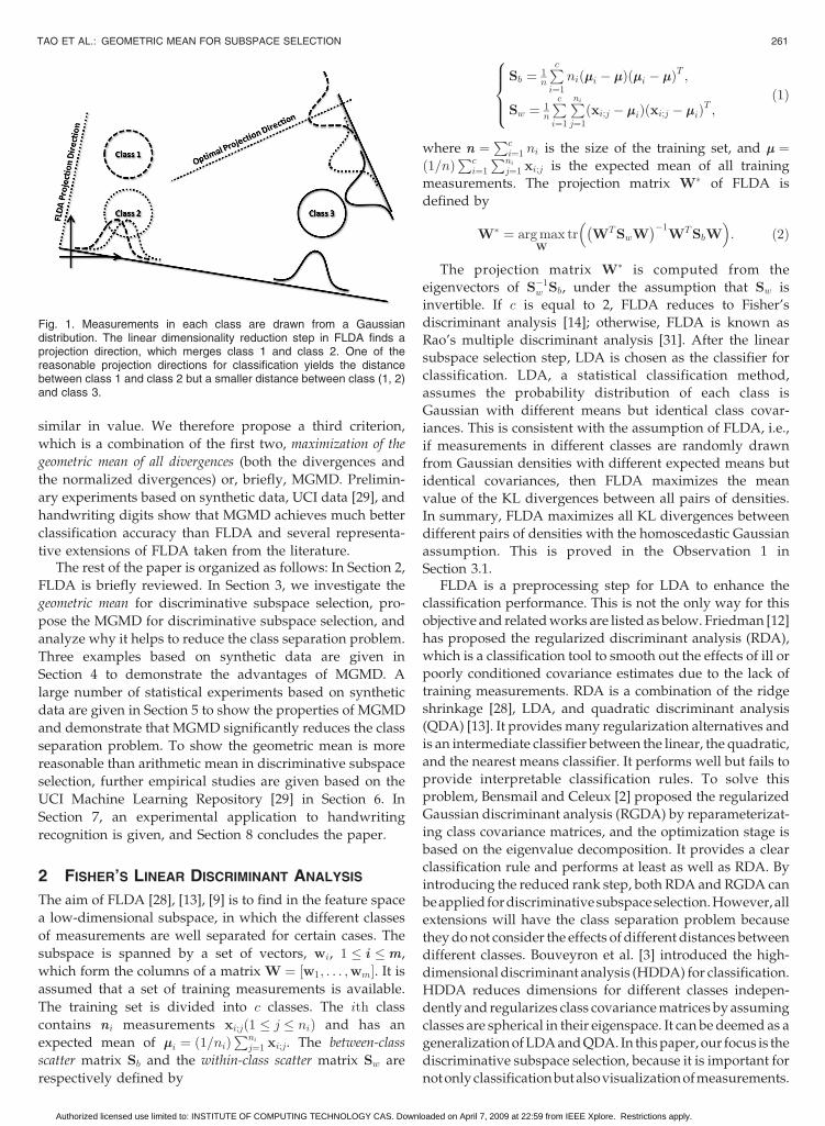
Fig. 1. Measurements in each class are drawn from a Gaussiandistribution. The linear dimensionality reduction step in FLDA finds aprojection direction, which merges class 1 and class 2. One of thereasonable projection directions for classification yields the distancebetween class 1 and class 2 but a smaller distance between class (1, 2)and class 3.


3 GEOMETRIC MEAN FOR SUBSPACE SELECTION

In FLDA, the arithmetic mean of the divergences is used tofind a suitable subspace into which to project the featurevectors. The main benefit of using the arithmetic mean isthat the projection matrix can be obtained by the general-ized eigenvalue decomposition. However, FLDA has theclass separation problem defined in Section 1, and it is notoptimal for multiclass classification [28], [23], [25], [27]because the effects of small divergences are not emphasizedin a proper way. This will merge two classes with a smalldivergence in the projected subspace so that large diver-gences can be preserved as much as possible to meet theobjective for subspace selection. To reduce this problem, thegeometric mean combined with the KL divergence iscarefully studied in this Section because this settingemphasizes effects of small divergences and thus reducesthe class separation problem significantly in the projectedsubspace. Moreover, the geometric mean can also beapplied to combine with Bregman divergence, as discussedin [37].

For Gaussian probability density functions, pi ¼ Nðx;��i;�iÞ, where ��i is the mean vector of the ith class measure-ments, and �i is the within-class covariance matrix of theith class, the KL divergence [5] is

D pikpj� �

¼ZdxN x;��i;�ið Þ ln N x;�i;�ið Þ

N x;��j;�j

� �¼ 1

2ln j�jj � ln j�ij þ tr ��1

j �i

� �þ tr ��1

j Dij

� �h i;

ð3Þ

where Dij ¼ ð��i � ��jÞð��i � ��jÞT and j�j ¼ detð�Þ. To sim-

plify the notation, we denote the KL divergence betweenthe projected densities pðWTxjy ¼ iÞ, and pðWTxjy ¼ jÞ:

DW pikpj� �

¼D p WTxjy ¼ i� �

kp WTxjy ¼ j� ��

¼ 1

2

�ln WT�jW�� ln WT�iW

�� þ tr WT�jW

� ��1WT �i þDij

� �W

� �� :

ð4Þ

3.1 General Averaged Divergence Analysis

We replace the arithmetic mean by the following generalmean,

V’ðWÞ ¼ ’�1

P1�i6¼j�c

qiqj’ DW pikpj� ��

P1�m 6¼n�c

qmqn

264

375; ð5Þ

where ’ð�Þ is a strict monotonic real-valued increasingfunction defined on ð0;þ1Þ; ’�1ð�Þ is the inverse functionof ’ð�Þ; qi is the prior probability of the ith class (usually, wecan set qi ¼ ni=n or simply set qi ¼ 1=c); pi is the conditionaldistribution of the ith class; x 2 RRn, where RRn is the featurespace containing the training measurements; and W 2Rn�k ðn � kÞ is the projection matrix. The general averageddivergence function measures the average of all divergencesbetween pairs of classes in the subspace. We obtain the

projection matrix W� by maximizing the general averaged

divergence function V’ðWÞ over W for a fixed ’ð�Þ.On setting ’ðxÞ ¼ x in (5), we obtain the arithmetic

mean-based method for choosing a subspace:

W� ¼ arg maxW

X1�i6¼j�c

qiqjDW pikpj� �P

1�m 6¼n�cqmqn

¼ arg maxW

X1�i6¼j�c

qiqjDW pikpj� �

:

ð6Þ

Observation 1. FLDA maximizes the arithmetic mean of the KL

divergences between all pairs of classes, under the assumption

that the Gaussian distributions for the different classes all have

the same covariance matrix. The projection matrix W� in

FLDA can be obtained by maximizing a particular VV ’ðWÞ.Proof. According to (3) and (4), the KL divergence between

the ith class and the jth class in the projected subspace

with the assumption of equal covariance matrices ð�i ¼�j ¼ �Þ is

DW pikpj� �

¼ 1

2tr WT�W� ��1

WTDijW� �

þ constant: ð7Þ

Then, we have

W� ¼ arg maxW

X1�i 6¼j�c

qiqjDW pikpj� �

¼ arg maxW

X1�i 6¼j�c

qiqjtr WT�W� ��1

WTDijW� ��

¼ arg maxW

tr WT�W� ��1

WTXc�1

i¼1

Xcj¼iþ1

qiqjDij

!W

!:

Because Sb ¼Pc�1

i¼1

Pcj¼iþ1 qiqjDij, as proved by Loog

in [24], and St ¼ Sb þ Sw ¼ � (see [13]), we have

arg maxW

X1�i6¼j�c

qiqjDW pikpj� �

¼ arg maxW

tr WTSwW� ��1

WTSbW� �

:ð8Þ

tu

It follows from (8) that a solution of FLDA can be

obtained by the generalized eigenvalue decomposition.

Example. Decell and Mayekar [8] maximize the summation

of all symmetric KL divergences between all pairs of

classes in the projected subspace. In essence, there is no

difference between [8] and maximizing the arithmetic

mean of all KL divergences.

3.2 Criterion 1: Maximization of the Geometric Meanof the Divergences

The log function is a suitable choice for ’ because it increases

the effects of the small divergences and, at the same time,

reduces the effects of the large divergences. On setting’ðxÞ ¼logðxÞ in (5), the generalized geometric mean of the diver-

gences is obtained. The required subspace W� is given by



W� ¼ arg maxW

Y1�i6¼j�c

DW pikpj� � qiqjP

1�m6¼n�cqmqn

: ð9Þ

It follows from the mean inequality that the generalized

geometric mean is upper bounded by the arithmetic mean

of the divergences, i.e.,

Y1�i 6¼j�c


1�m6¼n�cqmqn

�X

1�i6¼j�c

qiqjP1�m6¼n�c

qmqnDW pikpj

� �0B@

1CA:

ð10Þ

Furthermore, (9) emphasizes the total volume of all

divergences, e.g., in the special case qi ¼ qj for all i, j:

arg maxW

Y1�i6¼j�c


1�m6¼n�cqmqn

¼ arg maxW

Y1�i6¼j�c

DW pikpj� � qiqj

¼ arg maxW

Y1�i6¼j�c

DW pikpj� �

:

ð11Þ

3.3 Criterion 2: Maximization of the Geometric Meanof the Normalized Divergences

We can further strengthen the effects of the small

divergences on the selected subspace by maximizing the

geometric mean1 of all normalized divergences2 in the

projected subspace, i.e.,

W� ¼ arg maxW

Y1�i 6¼j�c

EW pikpj� �" # 1

cðc�1Þ

¼ arg maxW

Y1�i6¼j�c

EW pikpj� �

;

ð12Þ

where the normalized divergence EWðpikpjÞ between the

ith class and the jth class is defined by

EW pikpj� �

¼qiqjDW pikpj

� �P1�m 6¼n�c

qmqnDW pmkpnð Þ : ð13Þ

The intuition behind (12) is that the product of the

normalized divergences achieves its maximum value if and

when the normalized divergences are equal to each other.

Therefore, maximizing the geometric mean of the normal-

ized divergences tends to make the normalized divergences

as similar as possible. And, thus, the effects of the small

divergences are further emphasized.

3.4 Criterion 3: Maximization of the Geometric Meanof All Divergences

Although criterion 2 emphasizes the small divergencesduring optimization, direct use of this criterion is not

desirable for subspace selection. This is because experi-ments in Section 4.1 show that there exist W for which allthe divergences become small, but all the normalizeddivergences are comparable in value. In such cases, theprojection matrix W is unsuitable for classification, becauseseveral classes may be severely overlapped.

To reduce this problem, we combine criterion 2 withcriterion 1. The new criterion maximizes the linear combina-tion of 1) the log of the geometric mean of the divergences and2) the log of the geometric mean of the normalizeddivergences. This criterion is named the MGMD:

W� ¼ arg maxW

(� log

Y1�i6¼j�c

EW pikpj� �" # 1

cðc�1Þ

þð1� �Þ log

Y1�i6¼j�c


1�m6¼n�cqmqn

)

¼ arg maxW

1cðc�1Þ

P1�i6¼j�c

logDW pikpj� �

� logP

1�i6¼j�cqiqjDW pikpj

� � !

þ ð1��Þ�P

1�m6¼n�cqmqn

P1�i6¼j�c

qiqj logDW pikpj� �

8>>>>>>>><>>>>>>>>:

9>>>>>>>>=>>>>>>>>;;

ð14Þ

where the supremum of � is 1, and the infimum of � is 0.When � ¼ 0, (14) reduces to (9); and when � ¼ 1, (14)reduces to (12). By setting qi ¼ 1=c, we can simplify theabove formula as

W� ¼ arg maxW

( X1�i6¼j�c

logDW pikpj� �

� �cðc� 1Þ

logX

1�i 6¼j�cDW pikpj

� � !):

Based on (14), we define the value of the objectivefunction as

LðWÞ ¼ 1

cðc� 1ÞX

1�i6¼j�clogDW pikpj

� �

� logX

1�i6¼j�cqiqjDW pikpj

� � !

þ ð1� �Þ�

P1�m6¼n�c

qmqn

X1�i6¼j�c

qiqj logDW pikpj� �

:

ð15Þ

Therefore, W� ¼ arg maxW LðWÞ. The objective functionLðWÞ depends only on the subspace spanned by thecolumns of W or LðWÞ ¼ LðWQÞ when Q is an orthogonalr� r matrix. This is because DWðpikpjÞ ¼ DWQðpikpjÞaccording to [5] and [13]. In Section 3.5, we discuss howto obtain solutions for (14) based on the gradient steepestascent optimization procedure.

3.5 Optimization Procedure of MGMD

The gradient steepest ascent could be applied here to obtaina solution of MGMD. That is, the projection matrix can beupdated iteratively according to W Wþ � � @WLðWÞ,


1. In (12), we use the geometric mean but not the generalized geometricmean because the weights (the prior probabilities qi) are moved to thenormalized divergences, as shown in (13).

2. The sum of all normalized divergences is one.


where � is the learning rate parameter, and it affects thelearning procedure. If � is very small, it takes a largenumber of iterations to obtain a local optimal solution forthe projection matrix W. This means the training procedurewill be time consuming. Otherwise, the training procedurefails to converge to a local optimal solution for theprojection matrix W. To find a suitable � is not easy. Inthis paper, we just set it as a small value as 0.001 toguarantee the convergence of the training stage. To obtainthe optimization procedure for MGMD, we need the first-order derivative of LðWÞ,

@WLðWÞ ¼

P1�i6¼j�c

1cðc�1Þ þ

ð1��Þqiqj�P

1�m6¼n�cqmqn

0@

1AD�1

W pikpj� �

@WDW pikpj� �

�P

1�m6¼n�cqmqnDW pmkpnð Þ

!�1 P1�i6¼j�c

qiqj@WDW pikpj� � !

0BBBBBB@

1CCCCCCA;

ð16Þ

and

@WDW pikpj� �

¼

�jW WT�jW� ��1��iW WT�iW

� ��1þ

�i þDij

� �W WT�jW� ��1

��jW WT�jW� ��1

WT �i þDij

� �W WT�jW� ��1

0BB@

1CCA:ð17Þ

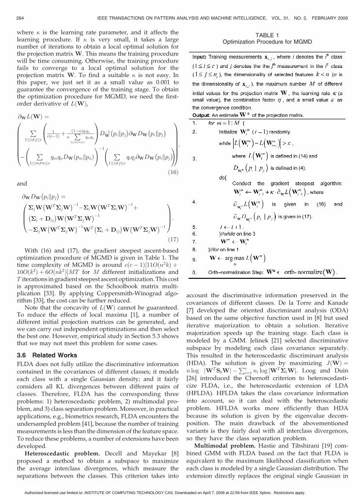
With (16) and (17), the gradient steepest ascent-basedoptimization procedure of MGMD is given in Table 1. Thetime complexity of MGMD is around cðc� 1Þ½11Oðn2kÞ þ10Oðk3Þ þ 6Oðnk2Þ�MT for M different initializations andT iterations in gradient steepest ascent optimization. This costis approximated based on the Schoolbook matrix multi-plication [33]. By applying Coppersmith-Winograd algo-rithm [33], the cost can be further reduced.

Note that the concavity of LðWÞ cannot be guaranteed.To reduce the effects of local maxima [1], a number ofdifferent initial projection matrices can be generated, andwe can carry out independent optimizations and then selectthe best one. However, empirical study in Section 5.3 showsthat we may not meet this problem for some cases.

3.6 Related Works

FLDA does not fully utilize the discriminative informationcontained in the covariances of different classes; it modelseach class with a single Gaussian density; and it fairlyconsiders all KL divergences between different pairs ofclasses. Therefore, FLDA has the corresponding threeproblems: 1) heteroscedastic problem, 2) multimodal pro-blem, and 3) class separation problem. Moreover, in practicalapplications, e.g., biometrics research, FLDA encounters theundersampled problem [41], because the number of trainingmeasurements is less than the dimension of the feature space.To reduce these problems, a number of extensions have beendeveloped.

Heteroscedastic problem. Decell and Mayekar [8]proposed a method to obtain a subspace to maximizethe average interclass divergences, which measure theseparations between the classes. This criterion takes into

account the discriminative information preserved in thecovariances of different classes. De la Torre and Kanade[7] developed the oriented discriminant analysis (ODA)based on the same objective function used in [8] but usediterative majorization to obtain a solution. Iterativemajorization speeds up the training stage. Each class ismodeled by a GMM. Jelinek [21] selected discriminativesubspace by modeling each class covariance separately.This resulted in the heteroscedastic discriminant analysis(HDA). The solution is given by maximizing JðWÞ ¼n log jWTSbWj �

Pci¼1 ni log jWT�iWj. Loog and Duin

[26] introduced the Chernoff criterion to heteroscedasti-cize FLDA, i.e., the heteroscedastic extension of LDA(HFLDA). HFLDA takes the class covariance informationinto account, so it can deal with the heteroscedasticproblem. HFLDA works more efficiently than HDAbecause its solution is given by the eigenvalue decom-position. The main drawback of the abovementionedvariants is they fairly deal with all interclass divergences,so they have the class separation problem.

Multimodal problem. Hastie and Tibshirani [19] com-bined GMM with FLDA based on the fact that FLDA isequivalent to the maximum likelihood classification wheneach class is modeled by a single Gaussian distribution. Theextension directly replaces the original single Gaussian in


TABLE 1Optimization Procedure for MGMD


each class by a Gaussian mixture model (GMM) inCampbell’s result [4]. De la Torre and Kanade [7] general-ized ODA for a multimodal case as the multimodal ODA(MODA) by combining it with the GMMs learned bynormalized cut [34].

Class separation problem. Lotlikar and Kothari [23]found for discriminative subspace selection that it isimportant to consider the nonuniform distances betweenclasses, i.e., some distances between different classes aresmall, while others are large. To take this information intoaccount, weightings are updated iteratively. According tothe analysis for the class separation problem, weightings arehelpful to reduce the class separation problem. It is worthnoting that Lotlikar and Kothari did not mention thisproblem formally, and polynomial functions over distancesbetween different classes are applied as weightings in aheuristic way. Unlike [23], Loog et al. [25] claimed thatð1=2x2Þerfðx=2

ffiffiffi2pÞ is a suitable weighting function, and x is

the distance between two classes weighted by the inverse ofthe total covariance matrix. In Loog’s weighting scheme,iterative optimization procedure is avoided and eigenvaluedecomposition is applied to have the projection matrix forsubspace selection. Moreover, Loog et al. proved that theirproposed criterion approximates the mean classificationaccuracy. However, both methods have the class separationproblem with the heteroscedastic setting, as demonstratedin Section 4.3, and it is difficult to extend them directly forheteroscedastic setting.

Undersampled problem. Friedman [12] proposed theRDA, which is a combination of ridge shrinkage, LDA, andQDA. Hastie et al. [17] viewed FLDA as multivariate linearregression and used the penalized least squares regressionto reduce the SSS problem. Swets and Weng [36] introducedPCA as the preprocessing step in FLDA for face recognition.Raudys and Duin [32] applied the pseudoinverse to thecovariance matrix in FLDA to reduce this problem. Ye et al.[41] introduced the generalized singular value decomposi-tion (GSVD) to avoid this problem in FLDA. Ye and Li [42]combined the orthogonal triangular decomposition withFLDA to reduce the SSS problem.

Nonparametric models. Recently, to take the nonlinearityof the measurement distribution into account, classificationdriven nonparametric models have been developed andachieved improvements. Hastie and Tibshirani [20] realizedthat the nearest neighbor classifier suffers from bias in high-dimensional space, and this affects the classification accu-racy. To reduce this problem, LDA is applied locally toestimate the local distance metric to estimate neighborhoodmeasurements for future classification. By reformulating thewithin-class scatter matrix and the between-class scatter matrixdefined in FLDA in a pairwise manner, Sugiyama [35]proposed the local FLDA (LFLDA). The original objective ofLFLDA is to reduce the multimodal problem in FLDA.Torkkola [40] applied the nonparametric Renyi entropy tomodel the mutual information between measurements in theselected subspace and corresponding labels. Because themutual information is relevant to the upper bound of theBayes error rate, it can be applied to select discriminativesubspaces. Fukumizu et al. [15] developed the kerneldimensionality reduction (KDR) based on the estimationand optimization of a particular class of operators on the

reproducing kernel Hilbert space, which provides character-izations of general notions of independence. These character-izations are helpful to design objective functions fordiscriminative subspace selection. Peltonen and Kaski [30]generalized FLDA through a probabilistic model by max-imizing mutual information. Unlike [40], they appliedShannon entropy for probabilistic inference. This model isequivalent to maximizing the mutual information withclasses asymptotically. Zhu and Hastie [44] developed ageneral model for discriminative subspace selection withoutassuming class densities belong to a particular family. Withnonparametric density estimators, this model maximizes thelikelihood ratio between class-specific and class-independentmodels. Goldberger et al. [16] developed the neighborhoodcomponents analysis (NCA) for learning a distance metric forthe k-nearest-neighbor ðkNNÞ classification. It maximizes astochastic variant of the leave-one-out kNN score overtraining measurements, and it is a nonparametric classifica-tion driven subspace selection method. Although nonpara-metric models achieve improvements for classification anddo not assume class densities belong to any particular family,it is still important to study models with specific priorprobability models for understanding statistical properties ofmeasurements. In addition, the new method could inprinciple be faster than several nonparametric methods sinceit only uses the covariance and Dij matrices for optimization,not the individual data point locations.

4 A COMPARATIVE STUDY USING SYNTHETIC DATA

In this section, we compare the effectiveness of MGMD withFLDA [13], HDA [21], aPAC [25], weighted FLDA(WFLDA) [13], FS-FLDA [23], HFLDA [26], ODA [7], andMODA [7] in handling three typical problems (heterosce-dastic problem, multimodal problem, and class separationproblem) appeared in FLDA. WFLDA [13] is similar toaPAC, but the weighting function is d�8, where d is theoriginal-space distance between a pair of class centers. InFS-FLDA, the weighting function is d�8, and the number offractional steps is 30. We denote the proposed method asMGMDð�Þ, where � is the combination factor defined in(14). The empirical studies in this section demonstrate thatMGMD has no heteroscedastic problem; the multimodalextension of MGMD has no multimodal problem, andMGMD can significantly reduce the class separationproblem. To better understand differences of these algo-rithms and to visualize measurements conveniently, mea-surements are generated in two-dimensional (2D) spaces. Inthe following experiments, projections with less classifica-tion errors are better choices as a classification goal becausethey better separate classes in the projected subspace. Wechoose the nearest class for each measurement by Mahala-nobis distance to the class center for classification.

4.1 Heteroscedastic Example

To examine the classification ability of these subspaceselection methods for the heteroscedastic problem [26], wegenerate two classes such that each class has 500 measure-ments, drawn from a Gaussian distribution. The two classeshave identical mean values but different covariances. Asshown in Fig. 2, FLDA, aPAC, WFLDA, and FS-FLDAseparate class means without taking the differences



between covariances into account. In contrast, HDA,

HFLDA, ODA, MGMD(0), and MGMD(1/2) consider both

the differences between class means and the differences

between class covariances, so they have less training errors,

and their projections are better in a classification goal.Based on the same data set, we demonstrate that the

geometric mean of the normalized divergences is not

sufficient for subspace selection. On setting � ¼ 1 in (14),

MGMD reduces to the maximization of the geometric mean

of the normalized KL divergences. Fig. 3a shows the

projection direction (indicated again by lines, as in Fig. 2)

of the training data from the 2D subspace to one-

dimensional (1D) space found by maximizing the geometric

mean of the normalized KL divergences, and the projection

direction will mix the two classes. Fig. 3b shows the

geometric mean of the normalized KLD in the 1D subspace

during training. From this experiment, we observe that

1) the KLD between class 1 and class 2 is 1.1451, and the

normalized KLD is 0.5091 at the 1,000th training iteration,

and 2) the KLD between class 2 and class 1 is 1.1043, and the

normalized KLD is 0.4909 at the 1,000th training iteration.

Fig. 3b shows that the normalized KL divergences is

maximized finally, but the Fig. 3a shows that the projection

direction is not suitable for classification. The suitable

projection direction for classification can be found in Fig. 2g.

4.2 Multimodal Example

In many applications, it is useful to model the distribution

of a class using a GMM, because measurements in the class

may be drawn from a non-Gaussian distribution. Themultimodal extension of MGMD (M-MGMD) is defined as

W� ¼ arg maxW

1cðc�1Þ

P1�i6¼j�c

P1�k�Ci

P1�l�Cj

log DW pki kplj� �h i

� logP

1�i6¼j�c

P1�k�Ci

P1�l�Cj

qki qlj DW pki kplj

� �h i" #

þ ð1��Þ�P

1�m6¼n�c

P1�k�Ci

P1�l�Cj

qkmqln

P1�i6¼j�c

P1�k�Ci

P1�l�Cj

qki qlj logDW pki kplj

� �h i

8>>>>>>>>>>>><>>>>>>>>>>>>:

9>>>>>>>>>>>>=>>>>>>>>>>>>;

;ð18Þ

where qki is the prior probability of the kth subcluster of theith class, pki is measurement probability of the kth subclusterin the ith class, andDWðpki kpljÞ is the divergence between thekth subcluster in the ith class and the lth subcluster in thejth class. The parameters for these subclusters can beobtained from the GMM-FJ method [11], which is a GMM-EM-like algorithm, proposed by Figueiredo and Jain. That is,we first run the GMM-FJ to obtain relevant parameters andthen apply (18) for discriminative subspace selection. Themerits of the incorporation of MGMD into GMM-FJ are givenas follows:

1. It reduces the class separation problem, defined inSection 1.

2. It inherits the merits of GMM-FJ [11]. In detail, itdetermines the number of subclusters in each classautomatically; it is less sensitive to the choice ofinitial values of the parameters than EM; and itavoids the boundary of the parameter space.

3. The objective function LGMMðWÞ is invariant torotation transformation.

To demonstrate the classification ability of M-MGMD,we generate two classes; each class has two subclusters; andmeasurements in each subcluster are drawn from aGaussian distribution. Fig. 4 shows the selected subspacesof different methods. In this case, FLDA, WFLDA, FS-FLDA, and aPAC do not select the suitable subspace forclassification. However, the multimodal extensions of ODAand MGMD can find the suitable subspace. Furthermore,although HDA and HFLDA do not take account ofmultimodal classes, they can select the suitable subspace.This is because in this case, the two classes have similarclass means but significantly different class covariancematrices when each class is modeled by a single Gaussian


Fig. 2. Heteroscedastic example: the projection directions (indicated bylines in each subfigure) obtained using (a) FLDA, (b) HDA, (c) aPAC,(d) WFLDA, (e) FS-FLDA, (f) HFLDA, (g) ODA, (h) MGMD(0), and(i) MGMD(1/2). The training errors of these methods, as measured byMahalanobis distance, are 0.3410, 0.2790, 0.3410, 0.3410, 0.3430,0.2880, 0.2390, 0.2390, and 0.2390, respectively. Therefore, HDA,HFLDA, ODA, MGMD(0), and MGMD(1/2) have less training errors inthis case.

Fig. 3. The maximization of the geometric mean of the normalized

divergences is insufficient for subspace selection.


distribution. For complex cases, e.g., when each class

consists of more than three subclusters, HDA and HFLDA

will fail to find the optimal subspace for classification.

4.3 Class Separation Problem

The most prominent advantage of MGMD is that it can

significantly reduce the classification errors caused by the

strong effects of the large divergences between certain

classes. To demonstrate this point, we generate three

classes, and measurements in each class are drawn from a

Gaussian distribution. Two classes are close together and

the third is further away.In this case, MGMD(0) can also reduce the problem, but

it cannot work as well as MGMD(5/6). In Fig. 5, MGMD(5/

6) shows a good ability of separating the last two classes of

measurements. Furthermore, in MGMD, we achieve the

same projection direction when setting � to 1/6, 2/6, 3/6,

4/6, and 5/6 for this data set. However, FLDA, HDA,

WFLDA, HFLDA, and ODA do not give good results. FS-

FLDA and aPAC algorithms are better than FLDA, but

neither of them gives the best projection direction.In Fig. 5, different Gaussians have identical class

covariances. In this case, FS-FLDA works better than aPAC.

In Fig. 6, different Gaussians have different class covar-

iances. In this case, aPAC works better than FS-FLDA.

Moreover, in both cases, the proposed MGMD(5/6)

achieves the best performance. Therefore, it is important

to consider the heteroscedastic problem and the class

separation problem simultaneously.

5 STATISTICAL EXPERIMENTS AND ANALYSIS

In this section, we utilize a synthetic data model, which is a

generalization of the data generation model used by Torre

and Kanade [7] to evaluate MGMD in terms of accuracy and

robustness. The accuracy is measured by the average error

rate and the robustness is measured by the standard

deviation of the classification error rates. In this data

generation model, there are five classes, which are repre-

sented by the symbols , �, þ, tu, and in Fig. 11. In our

experiments, for each of the training and testing sets, the data

generator gives 200 measurements for each of the five classes

(therefore, there are 1,000 measurements in total). Moreover,

the measurements in each class are obtained from a single

Gaussian. Each Gaussian density is a linear transformation of

a “standard normal distribution”. The linear transformations


Fig. 4. Multimodal problem: the optimal projection directions (indicatedby lines in each subfigure) by using (a) FLDA, (b) HDA, (c) aPAC,(d) WFLDA, (e) FS-FLDA, (f) HFLDA, (g) MODA, (h) M-MGMD(0), and(i) M-MGMD(1/2). The training errors measured by classificationaccording to the Mahalanobis distance to the nearest subcluster ofthese methods are 0.0917, 0.0167, 0.0917, 0.0917, 0.0917, 0.0167,0.0083, 0.0083, and 0.0083, respectively.

Fig. 5. Class separation problem: the projection directions (indicated bylines in each subfigure) by using (a) FLDA, (b) HDA, (c) aPAC,(d) WFLDA, (e) FS-FLDA, (f) HFLDA, (g) ODA, (h) MGMD(0), and(i) MGMD(5/6). The training errors measured by Mahalanobis distanceof these methods are 0.3100, 0.3033, 0.2900, 0.3033, 0.0567, 0.3100,0.3100, 0.1167, and 0.0200, respectively. MGMD(5/6) finds the bestprojection direction for classification.

Fig. 6. Class separation problem: the projection directions (indicated bylines in each subfigure) by using (a) aPAC, (b) FS-FLDA, and(c) MGMD(5/6). The training errors measured by Mahalanobis distanceof these methods are 0.1200, 0.1733, and 0.0267, respectively.MGMD(5/6) finds the best projection direction for classification.


are defined by xi;j ¼ Tizj þ ��i þ nj, where xi;j 2 R20,

Ti 2 R20�7, z � Nð0; IÞ 2 R7, n � Nð0; 2IÞ 2 R20, i denotes

the ith class, j denotes the jth measurement in this class, and

��i is the mean value of the corresponding normal distribu-

tion. The ��i are assigned as ��1 ¼ ð2Nð0; 1Þ þ 4Þ120, ��2 ¼ 020,

��3 ¼ ð2Nð0; 1Þ � 4Þ½010;110�T , ��4 ¼ ð2Nð0; 1Þ þ 4Þ½110;010�T ,

and ��5 ¼ ð2Nð0; 1Þ þ 4Þ½15;05;15;05�T . The projection matrix

Ti is a random matrix. Each of its elements is sampled from

Nð0; 5Þ. Based on this data generation model, 800 groups

(each group consists of the training and testing measure-

ments) of synthetic data are generated.For our comparative study, subspace selection methods,

e.g., MGMD, are first utilized to select a given number offeatures. Then, the nearest neighbor rule [9] and theMahalanobis distance [9] are used to examine the accuracyand the robustness of MGMD by comparing it with FLDAand its extensions. The baseline algorithms are FLDA [13],HDA [21], aPAC [25], WFLDA [13], FS-FLDA [23], LFLDA[35], HFLDA [26], and ODA [7]. For LFLDA, LFLDAachieved best performance by setting the metric as plaincompared with setting the metric as weighted andorthonormalized. Moreover, we set the kNN parameter to7 in LFLDA.

5.1 Performance Evaluation

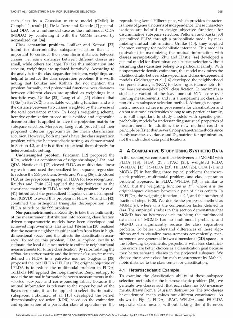
We conducted the designed experiments 800 times based onrandomly generated data sets. The experimental results arereported in Tables 2, 3, 4, and 5. Tables 2 and 4 show theaverage error rates of FLDA, HDA, aPAC, WFLDA, FS-FLDA, LFLDA, HFLDA, ODA, MGMD(0) , andMGMDð2=ðc� 1ÞÞ, where c is the number of classes. Tables 2

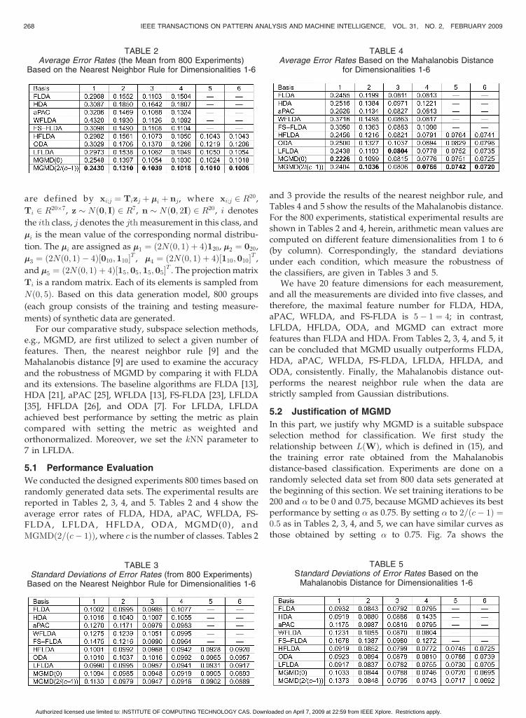
and 3 provide the results of the nearest neighbor rule, andTables 4 and 5 show the results of the Mahalanobis distance.For the 800 experiments, statistical experimental results areshown in Tables 2 and 4, herein, arithmetic mean values arecomputed on different feature dimensionalities from 1 to 6(by column). Correspondingly, the standard deviationsunder each condition, which measure the robustness ofthe classifiers, are given in Tables 3 and 5.

We have 20 feature dimensions for each measurement,and all the measurements are divided into five classes, andtherefore, the maximal feature number for FLDA, HDA,aPAC, WFLDA, and FS-FLDA is 5� 1 ¼ 4; in contrast,LFLDA, HFLDA, ODA, and MGMD can extract morefeatures than FLDA and HDA. From Tables 2, 3, 4, and 5, itcan be concluded that MGMD usually outperforms FLDA,HDA, aPAC, WFLDA, FS-FLDA, LFLDA, HFLDA, andODA, consistently. Finally, the Mahalanobis distance out-performs the nearest neighbor rule when the data arestrictly sampled from Gaussian distributions.

5.2 Justification of MGMD

In this part, we justify why MGMD is a suitable subspaceselection method for classification. We first study therelationship between LðWÞ, which is defined in (15), andthe training error rate obtained from the Mahalanobisdistance-based classification. Experiments are done on arandomly selected data set from 800 data sets generated atthe beginning of this section. We set training iterations to be200 and � to be 0 and 0.75, because MGMD achieves its bestperformance by setting � as 0.75. By setting � to 2=ðc� 1Þ ¼0:5 as in Tables 2, 3, 4, and 5, we can have similar curves asthose obtained by setting � to 0.75. Fig. 7a shows the


TABLE 2Average Error Rates (the Mean from 800 Experiments)

Based on the Nearest Neighbor Rule for Dimensionalities 1-6

TABLE 3Standard Deviations of Error Rates (from 800 Experiments)

Based on the Nearest Neighbor Rule for Dimensionalities 1-6

TABLE 4Average Error Rates Based on the Mahalanobis Distance

for Dimensionalities 1-6

TABLE 5Standard Deviations of Error Rates Based on the

Mahalanobis Distance for Dimensionalities 1-6


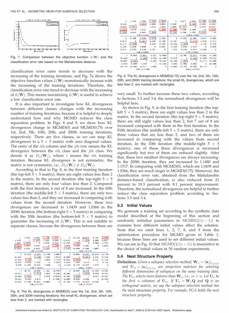
classification error rates trends to decrease with theincreasing of the training iterations, and Fig. 7a shows theobjective function values LðWÞmonotonically increase withthe increasing of the training iterations. Therefore, theclassification error rate trend to decrease with the increasingof LðWÞ. This means maximizing LðWÞ is useful to achievea low classification error rate.

It is also important to investigate how KL divergencesbetween different classes changes with the increasingnumber of training iterations, because it is helpful to deeplyunderstand how and why MGMD reduces the classseparation problem. In Figs. 8 and 9, we show how KLdivergences change in MGMD(0) and MGMD(0.75) over1st, 2nd, 5th, 10th, 20th, and 200th training iterations,respectively. There are five classes, so we can map KLdivergences to a 5 � 5 matrix with zero diagonal values.The entry of the ith column and the jth row means the KLdivergence between the ith class and the jth class. Wedenote it as DijðWtÞ, where t means the tth trainingiteration. Because KL divergence is not symmetric, thematrix is not symmetric, i.e., DijðWtÞ 6¼ DjiðWtÞ.

According to that in Fig. 8, in the first training iteration(the top-left 5 � 5 matrix), there are eight values less than 2in the matrix. In the second iteration (the top-right 5 � 5matrix), there are only four values less than 2. Comparedwith the first iteration, 6 out of 8 are increased. In the fifthiteration (the middle-left 5 � 5 matrix), there are only twovalues less than 2, and they are increased in comparing withvalues from the second iteration. However, these twodivergences are decreased to 1.0439 and 1.0366 in the200th iteration (the bottom-right 5 � 5 matrix) in comparingwith the 20th iteration (the bottom-left 5 � 5 matrix) toguarantee the increasing of LðWÞ. This is not suitable toseparate classes, because the divergences between them are

very small. To further increase these two values, accordingto Sections 3.3 and 3.4, the normalized divergences will behelpful here.

As shown in Fig. 9, in the first training iteration (the top-left 5 � 5 matrix), there are eight values less than 2 in thematrix. In the second iteration (the top-right 5 � 5 matrix),there are still eight values less than 2, but 7 out of 8 areincreased compared with them in the first iteration. In theFifth iteration (the middle-left 5 � 5 matrix), there are onlythree values that are less than 2, and two of them areincreased in comparing with the values from seconditeration. In the 10th iteration (the middle-right 5 � 5matrix), one of these three divergences is increasedsignificantly but two of them are reduced slightly. Afterthat, these two smallest divergences are always increasing.In the 200th iteration, they are increased to 1.1480 and1.1517. In comparing with MGMD(0), which are 1.0439 and1.0366, they are much larger in MGMD(0.75). Moreover, theclassification error rate, obtained from the Mahalanobisdistance-based classification, is also reduced from 21percent to 19.3 percent with 8.1 percent improvement.Therefore, the normalized divergences are helpful to furtherreduce the class separation problem according to Sec-tions 3.3 and 3.4.

5.3 Initial Values

We generate a training set according to the synthetic datamodel described at the beginning of this section andrandomly initialize parameters in MGMDð2=ðc� 1ÞÞ toexamine how different initial values affect the solution.Note that we omit lines 1, 2, 7, 8, and 9 from theoptimization procedure for MGMD given in Table 1,because these lines are used to set different initial values.We can see in Fig. 10 that MGMDð2=ðc� 1ÞÞ is insensitive tothe choice of initial values in 50 random experiments.

5.4 Nest Structure Property

Definition. Given a subspace selection method, Wn ¼ ½wi�1�i�nand Um ¼ ½ui�1�i�m are projection matrices for selectingdifferent dimensions of subspaces on the same training data.The Um selects more features than Wn, i.e., m > n. Let Un bethe first n columns of Um. If Un ¼WnQ and Q is anorthogonal matrix, we say the subspace selection method hasthe nest structure property. For example, PCA holds the neststructure property.


Fig. 7. Comparison between the objective function LðWÞ and the

classification error rate based on the Mahalanobis distance.

Fig. 8. The KL divergences in MGMD(0) over the 1st, 2nd, 5th, 10th,

20th, and 200th training iterations: the small KL divergences, which are

less than 2, are marked with rectangles.

Fig. 9. The KL divergences in MGMD(0.75) over the 1st, 2nd, 5th, 10th,

20th, and 200th training iterations: the small KL divergences, which are

less than 2, are marked with rectangles.


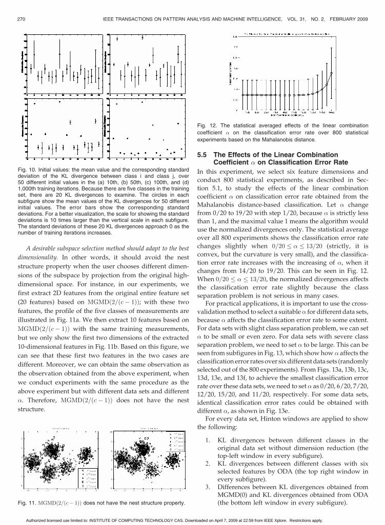
A desirable subspace selection method should adapt to the best

dimensionality. In other words, it should avoid the nest

structure property when the user chooses different dimen-

sions of the subspace by projection from the original high-

dimensional space. For instance, in our experiments, we

first extract 2D features from the original entire feature set

(20 features) based on MGMDð2=ðc� 1ÞÞ; with these two

features, the profile of the five classes of measurements are

illustrated in Fig. 11a. We then extract 10 features based on

MGMDð2=ðc� 1ÞÞ with the same training measurements,

but we only show the first two dimensions of the extracted

10-dimensional features in Fig. 11b. Based on this figure, we

can see that these first two features in the two cases are

different. Moreover, we can obtain the same observation as

the observation obtained from the above experiment, when

we conduct experiments with the same procedure as the

above experiment but with different data sets and different

�. Therefore, MGMDð2=ðc� 1ÞÞ does not have the nest

structure.

5.5 The Effects of the Linear CombinationCoefficient � on Classification Error Rate

In this experiment, we select six feature dimensions and

conduct 800 statistical experiments, as described in Sec-

tion 5.1, to study the effects of the linear combination

coefficient � on classification error rate obtained from the

Mahalanobis distance-based classification. Let � change

from 0/20 to 19/20 with step 1/20, because � is strictly less

than 1, and the maximal value 1 means the algorithm would

use the normalized divergences only. The statistical average

over all 800 experiments shows the classification error rate

changes slightly when 0=20 � � � 13=20 (strictly, it is

convex, but the curvature is very small), and the classifica-

tion error rate increases with the increasing of �, when it

changes from 14/20 to 19/20. This can be seen in Fig. 12.

When 0=20 � � � 13=20, the normalized divergences affects

the classification error rate slightly because the class

separation problem is not serious in many cases.For practical applications, it is important to use the cross-

validation method to select a suitable� for different data sets,

because � affects the classification error rate to some extent.

For data sets with slight class separation problem, we can set

� to be small or even zero. For data sets with severe class

separation problem, we need to set � to be large. This can be

seen from subfigures in Fig. 13, which show how� affects the

classification error rates over six different data sets (randomly

selected out of the 800 experiments). From Figs. 13a, 13b, 13c,

13d, 13e, and 13f, to achieve the smallest classification error

rate over these data sets, we need to set � as 0/20, 6/20, 7/20,

12/20, 15/20, and 11/20, respectively. For some data sets,

identical classification error rates could be obtained with

different �, as shown in Fig. 13e.For every data set, Hinton windows are applied to show

the following:

1. KL divergences between different classes in theoriginal data set without dimension reduction (thetop-left window in every subfigure).

2. KL divergences between different classes with sixselected features by ODA (the top right window inevery subfigure).

3. Differences between KL divergences obtained fromMGMD(0) and KL divergences obtained from ODA(the bottom left window in every subfigure).


Fig. 10. Initial values: the mean value and the corresponding standarddeviation of the KL divergence between class i and class j, over50 different initial values in the (a) 10th, (b) 50th, (c) 100th, and (d)1,000th training iterations. Because there are five classes in the trainingset, there are 20 KL divergences to examine. The circles in eachsubfigure show the mean values of the KL divergences for 50 differentinitial values. The error bars show the corresponding standarddeviations. For a better visualization, the scale for showing the standarddeviations is 10 times larger than the vertical scale in each subfigure.The standard deviations of these 20 KL divergences approach 0 as thenumber of training iterations increases.

Fig. 11. MGMDð2=ðc� 1ÞÞ does not have the nest structure property.

Fig. 12. The statistical averaged effects of the linear combination

coefficient � on the classification error rate over 800 statistical

experiments based on the Mahalanobis distance.


4. Differences between KL divergences obtained fromMGMD(�) and KL divergences obtained from ODA(the bottom right window in every subfigure).

Because there are five classes, KL divergences are mappedto a 5 � 5 matrix with zero diagonal values. The size of a

block represents the value of the entry. The larger of theblock is, the larger of the absolute value of the correspond-ing entry is. The green (light) block means the entry ispositive, and the red (dark) block means the entry isnegative.

Based on these Hinton windows, small divergences inMGMD(0) are always larger than the correspondingdivergences in ODA indicated by green (light) color in thebottom Hinton diagrams in each subfigure, and large

divergences in MGMD(0) are always smaller than thecorresponding divergences in ODA indicated by red (dark)color in the bottom Hinton diagrams in each subfigure.Moreover, the MGMDð�Þ helps to further enlarge smalldivergences in the projected low-dimensional subspace,and the cost is the large divergences are further reduced.This is because the normalized divergences are taken intoaccount. Although large � is helpful to enlarge smalldivergences in subspace selection, some classes will be

merged together, and this enlarges the classification error.Therefore, with suitable � in MGMD, small divergences willbe enlarged suitably for discriminative subspace selection.

5.6 KL Divergence versus SymmetricKL Divergence

In this part, we compare the KL divergence with thesymmetric divergence in classification based on theproposed MGMD. With (3), the symmetric KL divergence is

S pikpj� �

¼ 1

2D pikpj� �

þD pjkpi� �

¼ 1

4

�tr ��1

j �i

� �þ tr ��1

i �j

� �þ tr ��1

j þ��1i

� �Dij

� ��:

ð19Þ

To simplify the notation, we denote the symmetric KLdivergence between the projected densities pðWTxjy ¼ iÞand pðWTxjy ¼ jÞ by

SW pikpj� �

¼S p WTxjy ¼ i� �

kp WTxjy ¼ j� ��

¼ 1

4

�tr WT�jW� ��1

WT �i þDij

� �W

� ��

þ tr WT�iW� ��1

WT �j þDij

� �W

� �� :

ð20Þ

Therefore, (14) changes to

W� ¼ arg maxW

1cðc�1Þ

P1�i6¼j�c

logSW pikpj� �

� logP

1�m 6¼n�cqmqnSW pmkpnð Þ

!

þ ð1��Þ�P

1�m6¼n�cqmqn

P1�i6¼j�c

qiqj logSW pikpj� �

8>>>>>>>><>>>>>>>>:

9>>>>>>>>=>>>>>>>>;;

ð21Þ

where the supremum of � is 1, and the infimum of � is 0.When � ¼ 0, (14) reduces to (9); and when � ¼ 1, (14)reduces to (12).

For empirical justification, experiments are conducted on800 data sets for both KL divergence-based and symmetric KLdivergence-based MGMD, and the linear combinationcoefficient � changes from 0/20 to 19/20 with step 1/20.Therefore, two matrices E1 and E2 with size 800 � 20 areobtained the entries ofE1 andE2 store the classification errorrate, which is obtained from the Mahalanobis distance-basedclassification, for a specific data set and a specific � for KLdivergence-based and symmetric KL divergence-basedMGMD, respectively. Fig. 14a describes the error barinformation of the difference between E1 and E2, i.e.,E1 �E2, over different �. This figure shows the difference isvery small in terms of classification error rates between KLdivergence-based and symmetric divergence-based MGMDwhen � changes from 0/20 to 13/20. When � changes from14/20 to 19/20, the difference is a little large. These twoobservations are based on the length of the correspondingerror bars. In Fig. 15b, we show this point based on somespecific data sets. In this figure, the x-coordinate representsrandomly selected 40 data sets, and the y-coordinaterepresents the difference of the classification error rates,obtained from the Mahalanobis distance-based classification,


Fig. 13. The effects of the linear combination coefficient � on theclassification error rate over six different data sets based on theMahalanobis distance. To achieve the smallest classification error rateover these data sets, we need to set � as (a) 0/20, (b) 6/20, (c) 7/20,(d) 12/20, (e) 15/20, and (f) 11/20, respectively.

Fig. 14. (a) The difference of the classification error rates, which areobtained from the Mahalanobis distance-based classification over800 data sets, between KL divergence-based and symmetric KL (SKL)divergence-based MGMD over different linear combination coefficient �,which changes from 0/20 to 19/20. (b) The difference of theclassification error rates, which are obtained from the Mahalanobisdistance-based classification over 800 data sets, between KL diver-gence-based and symmetric KL divergence-based MGMD for randomlyselected data sets (the error bar is the standard deviation obtained fromdifferent �).


between KL divergence-based and symmetric KL diver-gence-based MGMD. The error bars in the right subfigure arecalculated over different �, which changes from 0/20 to 19/20. Usually, the difference of the classification error ratesbetween KL divergence-based and symmetric KL diver-gence-based MGMD is very small because averaged differ-ence over different � is almost zero, and the correspondingerror bar is short for different data sets. However, for the 9th,18th, 24th, 26th, and 35th data sets here, the averageddifferences are not zero, and the corresponding standarddeviations are large. Therefore, the cross validation could bealso applied to select suitable divergence, i.e., KL divergenceor symmetric KL divergence.

6 EXPERIMENTS WITH UCI MACHINE LEARNING

REPOSITORY

To justify the significance of the geometric mean forsubspace selection, we conduct experiments to compareMGMDð0=�Þ with ODA over six data sets in the UCIMachine Learning Repository [29]. In all experiments, weset � to be 2=c, and the nearest neighbor rule is applied forclassification. Variations on the averaged classificationerrors are obtained from conventional fivefold crossvalidation over different random runs, i.e., measurementsin each data set are divided into five folds, and one fold isused for testing and the rest for training in each turn.

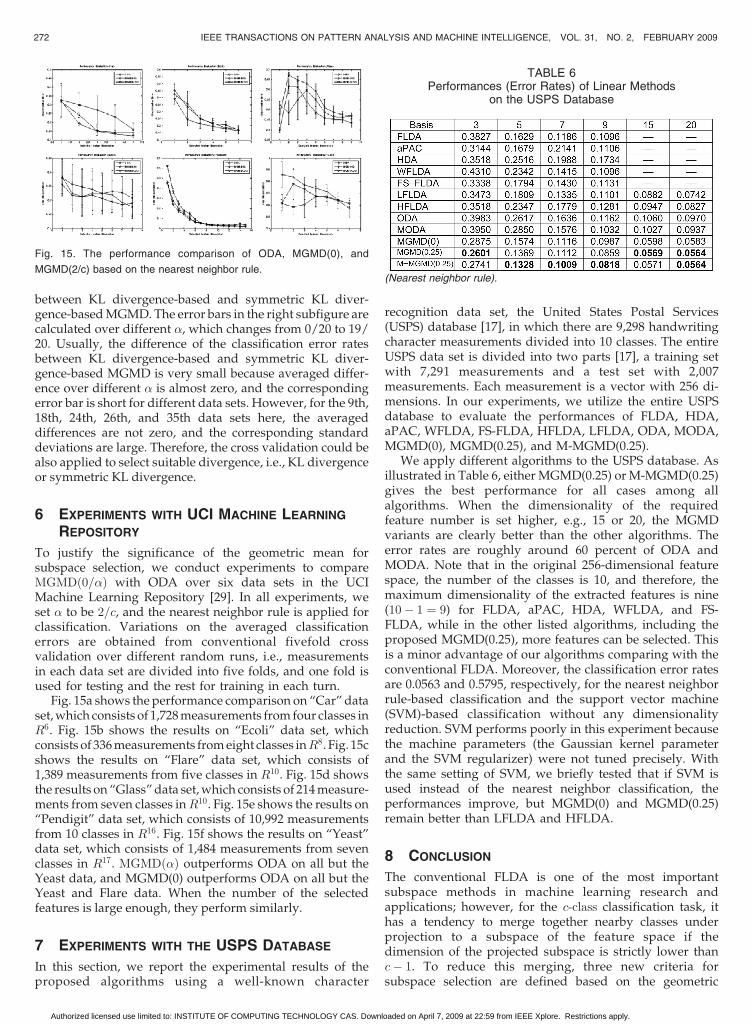
Fig. 15a shows the performance comparison on “Car” dataset, which consists of 1,728 measurements from four classes inR6. Fig. 15b shows the results on “Ecoli” data set, whichconsists of 336 measurements from eight classes inR8. Fig. 15cshows the results on “Flare” data set, which consists of1,389 measurements from five classes in R10. Fig. 15d showsthe results on “Glass” data set, which consists of 214 measure-ments from seven classes inR10. Fig. 15e shows the results on“Pendigit” data set, which consists of 10,992 measurementsfrom 10 classes in R16. Fig. 15f shows the results on “Yeast”data set, which consists of 1,484 measurements from sevenclasses in R17. MGMDð�Þ outperforms ODA on all but theYeast data, and MGMD(0) outperforms ODA on all but theYeast and Flare data. When the number of the selectedfeatures is large enough, they perform similarly.

7 EXPERIMENTS WITH THE USPS DATABASE

In this section, we report the experimental results of theproposed algorithms using a well-known character

recognition data set, the United States Postal Services(USPS) database [17], in which there are 9,298 handwritingcharacter measurements divided into 10 classes. The entireUSPS data set is divided into two parts [17], a training setwith 7,291 measurements and a test set with 2,007measurements. Each measurement is a vector with 256 di-mensions. In our experiments, we utilize the entire USPSdatabase to evaluate the performances of FLDA, HDA,aPAC, WFLDA, FS-FLDA, HFLDA, LFLDA, ODA, MODA,MGMD(0), MGMD(0.25), and M-MGMD(0.25).

We apply different algorithms to the USPS database. Asillustrated in Table 6, either MGMD(0.25) or M-MGMD(0.25)gives the best performance for all cases among allalgorithms. When the dimensionality of the requiredfeature number is set higher, e.g., 15 or 20, the MGMDvariants are clearly better than the other algorithms. Theerror rates are roughly around 60 percent of ODA andMODA. Note that in the original 256-dimensional featurespace, the number of the classes is 10, and therefore, themaximum dimensionality of the extracted features is nine(10� 1 ¼ 9) for FLDA, aPAC, HDA, WFLDA, and FS-FLDA, while in the other listed algorithms, including theproposed MGMD(0.25), more features can be selected. Thisis a minor advantage of our algorithms comparing with theconventional FLDA. Moreover, the classification error ratesare 0.0563 and 0.5795, respectively, for the nearest neighborrule-based classification and the support vector machine(SVM)-based classification without any dimensionalityreduction. SVM performs poorly in this experiment becausethe machine parameters (the Gaussian kernel parameterand the SVM regularizer) were not tuned precisely. Withthe same setting of SVM, we briefly tested that if SVM isused instead of the nearest neighbor classification, theperformances improve, but MGMD(0) and MGMD(0.25)remain better than LFLDA and HFLDA.

8 CONCLUSION

The conventional FLDA is one of the most importantsubspace methods in machine learning research andapplications; however, for the c-class classification task, ithas a tendency to merge together nearby classes underprojection to a subspace of the feature space if thedimension of the projected subspace is strictly lower thanc� 1. To reduce this merging, three new criteria forsubspace selection are defined based on the geometric


Fig. 15. The performance comparison of ODA, MGMD(0), and

MGMD(2/c) based on the nearest neighbor rule.

TABLE 6Performances (Error Rates) of Linear Methods

on the USPS Database

(Nearest neighbor rule).


mean of the divergences between the different pairs ofclasses, namely, 1) maximization of the geometric mean of thedivergences, 2) maximization of the geometric mean of thenormalized divergences, and 3) MGMD. The third criterion isa combination of the first two criteria. The new subspaceselection algorithm has been tested experimentally usingsynthetic data, UCI Machine Learning Repository, andhandwriting digits from the USPS database. The experi-ments show that the third criterion, namely, the maximiza-tion of the geometric mean of all KL divergences, is moreeffective than FLDA and its representative extensions.

ACKNOWLEDGMENTS

The authors would like to thank the associate editorProfessor Mario Figueiredo and the four anonymousreviewers for their constructive comments on the first twoversions of this paper. The research was partially supportedby the Start-up Grant of the Nanyang TechnologicalUniversity (under account number M58020010).

REFERENCES

[1] S. Boyd and L. Vandenberghe, Convex Optimization. CambridgeUniv. Press, 2004.

[2] H. Bensmail and G. Celeux, “Regularized Gaussian DiscriminantAnalysis through Eigenvalue Decomposition,” J. Am. StatisticalAssoc., vol. 91, pp. 1743-1748, 1996.

[3] C. Bouveyron, S. Girard, and C. Schmid, “High DimensionalDiscriminant Analysis,” Comm. in Statistics: Theory and Methods,vol. 36, no. 14, p. 2007,

[4] N. Campbell, “Canonical Variate Analysis—A General Formula-tion,” Australian J. Statistics, vol. 26, pp. 86-96, 1984.

[5] T.M. Cover and J.A. Thomas, Elements of Information Theory. Wiley,1991.

[6] L.S. Daniel and J. Weng, “Hierarchical Discriminant Analysis forImage Retrieval,” IEEE Trans. Pattern Analysis and MachineIntelligence, vol. 21, no. 5, pp. 386-401, May 1999.

[7] F. De la Torre and T. Kanade, “Multimodal Oriented DiscriminantAnalysis,” Proc. Int’l Conf. Machine Learning, Aug. 2005.

[8] H.P. Decell and S.M. Mayekar, “Feature Combinations and theDivergence Criterion,” Computers and Math. with Applications,vol. 3, pp. 71-76, 1977.

[9] R.O. Duda, P.E. Hart, and D.G. Stork, Pattern Classification, seconded. John Wiley & Sons, 2001.

[10] S. Dudoit, J. Fridlyand, and T.P. Speed, “Comparison ofDiscrimination Methods for the Classification of Tumors UsingGene Expression Data,” J. Am. Statistical Assoc., vol. 97, no. 457,pp. 77-87, 2002.

[11] M. Figueiredo and A.K. Jain, “Unsupervised Learning of FiniteMixture Models,” IEEE Trans. Pattern Analysis and MachineIntelligence, vol. 24, no. 3, pp. 381-396, Mar. 2002.

[12] J.H. Friedman, “Regularized Discriminant Analysis,” J. Am.Statistical Assoc., vol. 84, pp. 165-175, 1989.

[13] K. Fukunaga, Introduction to Statistical Pattern Recognition, seconded. Academic Press, 1990.

[14] R.A. Fisher, “The Use of Multiple Measurements in TaxonomicProblems,” Annals of Eugenics, vol. 7, pp. 179-188, 1936.

[15] K. Fukumizu, F.R. Bach, and M.I. Jordan, “DimensionalityReduction for Supervised Learning with Reproducing KernelHilbert Spaces,” J. Machine Learning Research, vol. 5, pp. 73-99,2004.

[16] J. Goldberger, S. Roweis, G. Hinton, and R. Salakhutdinov,“Neighbourhood Components Analysis,” Neural Information Pro-cessing Systems, 2004.

[17] T. Hastie, A. Buja, and R. Tibshirani, “Penalized DiscriminantAnalysis,” Annals of Statistics, vol. 23, pp. 73-102, 1995.

[18] T. Hastie, R. Tibshirani, and J.H. Friedman, The Elements of StatisticalLearning: Data Mining, Inference, and Prediction. Springer, 2001.

[19] T. Hastie and R. Tibshirani, “Discriminant Analysis by GaussianMixtures,” J. Royal Statistical Soc. B: Methodological, vol. 58, pp. 155-176, 1996.

[20] T. Hastie and R. Tibshirani, “Discriminant Adaptive NearestNeighbor Classification,” IEEE Trans. Pattern Analysis and MachineIntelligence, vol. 18, no. 6, pp. 607-615, June 1996.

[21] B. Jelinek,, “Review on Heteroscedastic Discriminant Analysis,”unpublished report, Center for Advanced Vehicular Systems,Mississippi State Univ., 2001.

[22] T.K. Kim and J. Kittler, “Locally Linear Discriminant Analysis forMultimodally Distributed Classes for Face Recognition with aSingle Model Image,” IEEE Trans. Pattern Analysis and MachineIntelligence, vol. 27, no. 3, pp. 318-327, Mar. 2005.

[23] R. Lotlikar and R. Kothari, “Fractional-Step DimensionalityReduction,” IEEE Trans. Pattern Analysis and Machine Intelligence,vol. 22, no. 6, pp. 623-627, June 2000.

[24] M. Loog, Approximate Pairwise Accuracy Criteria for MulticlassLinear Dimension Reduction: Generalizations of the Fisher Criterion.Delft Univ. Press, 1999.

[25] M. Loog, R.P.W. Duin, and R. Haeb-Umbach, “Multiclass LinearDimension Reduction by Weighted Pairwise Fisher Criteria,”IEEE Trans. Pattern Analysis and Machine Intelligence, vol. 23, no. 7,pp. 762-766, July 2001.

[26] M. Loog and R.P.W. Duin, “Linear Dimensionality Reduction viaa Heteroscedastic Extension of LDA: The Chernoff Criterion,”IEEE Trans. Pattern Analysis and Machine Intelligence, vol. 26, no. 6,pp. 732-739, June 2004.

[27] J. Lu, K.N. Plataniotis, and A.N. Venetsanopoulos, “FaceRecognition Using LDA Based Algorithms,” IEEE Trans. NeuralNetworks, vol. 14, no. 1, pp. 195-200, Jan. 2003.

[28] G.J. McLachlan, Discriminant Analysis and Statistical PatternRecognition. Wiley, 1992.

[29] D.J. Newman, S. Hettich, C.L. Blake, and C.J. Merz, UCI Repositoryof Machine Learning Databases, Dept. Information and ComputerSciences, Univ. of California, http://www.ics.uci.edu/~mlearn/MLRepository.html, 1998.

[30] J. Peltonen and S. Kaski, “Discriminative Components of Data,”IEEE Trans. Neural Networks, vol. 16, pp. 68-83, 2005.

[31] C.R. Rao, “The Utilization of Multiple Measurements in Problemsof Biological Classification,” J. Royal Statistical Soc. B: Methodolo-gical, vol. 10, pp. 159-203, Oct. 1948.

[32] S. Raudys and R.P.W. Duin, “On Expected Classification Error ofthe Fisher Linear Classifier with Pseudo-Inverse CovarianceMatrix,” Pattern Recognition Letter, vol. 19, nos. 5-6, 1998.

[33] A. Schonhage, A.F.W. Grotefeld, and E. Vetter, Fast Algorithms-AMultitape Turing Machine Implementation. BI Wissenschafts, 1994.

[34] J. Shi and J. Malik, “Normalized Cuts and Image Segmentation,”IEEE Trans. Pattern Analysis and Machine Intelligence, vol. 22, no. 8,pp. 888-905, Aug. 2000.

[35] M. Sugiyama, “Dimensionality Reduction of Multimodal LabeledData by Local Fisher Discriminant Analysis,” J. Machine LearningResearch, vol. 8, pp. 1027-1061, 2007.

[36] D.L. Swets and J. Weng, “Using Discriminant Eigenfeatures forImage Retrieval,” IEEE Trans. Pattern Analysis and MachineIntelligence, vol. 18, no. 8, pp. 831-836, Aug. 1996.

[37] D. Tao, X. Li, X. Wu, and S.J. Maybank, “General AveragedDivergences Analysis,” Proc. IEEE Int’l Conf. Data Mining, 2007.

[38] D. Tao, X. Li, X. Wu, and S.J. Maybank, “General TensorDiscriminant Analysis and Gabor Features for Gait Recognition,”IEEE Trans. Pattern Analysis and Machine Intelligence, vol. 29, no. 10,pp. 1700-1715, Oct. 2007.

[39] D. Tao, X. Li, X. Wu, and S.J. Maybank, “Supervised TensorLearning,” Knowledge and Information Systems, vol. 13, no. 1, pp. 1-42, 2007.

[40] K. Torkkola, “Feature Extraction by Non-Parametric MutualInformation Maximization,” J. Machine Learning Research, vol. 3,pp. 1415-1438, 2003.

[41] J. Ye, R. Janardan, C.H. Park, and H. Park, “An OptimizationCriterion for Generalized Discriminant Analysis on Under-sampled Problems,” IEEE Trans. Pattern Analysis and MachineIntelligence, vol. 26, no. 8, pp. 982-994, Aug. 2004.

[42] J. Ye and Q. Li, “A Two-Stage Linear Discriminant Analysis viaQR-Decomposition,” IEEE Trans. Pattern Analysis and MachineIntelligence, vol. 27, no. 6, pp. 929-941, June 2005.

[43] H. Yu and J. Yang, “A Direct LDA Algorithm for High-Dimensional Data with Application to Face Recognition,” PatternRecognition, vol. 34, no. 12, pp. 2067-2070, Dec. 2001.

[44] M. Zhu and T. Hastie, “Feature Extraction for Non-ParametricDiscriminant Analysis,” J. Computational and Graphical Statistics,vol. 12, pp. 101-120, 2003.



Dacheng Tao received the BEng degree fromthe University of Science and Technology ofChina (USTC), the MPhil degree from theChinese University of Hong Kong (CUHK), andthe PhD degree from the University of London.Currently, he is a Nanyang assistant professor inthe School of Computer Engineering at theNanyang Technological University, a visitingprofessor at Xi Dian University, a guest professorat Wu Han University, and a visiting research

fellow at the University of London. His research is mainly on applyingstatistics and mathematics for data analysis problems in data mining,computer vision, machine learning, multimedia, and visual surveillance.He has published more than 90 scientific papers in journals includingIEEE Transactions on Pattern Analysis and Machine Intelligence, IEEETransactions on Knowledge and Data Engineering, IEEE Transactionson Image Processing, etc., with best paper runner up awards. Previously,he gained several Meritorious Awards from the International Interdisci-plinary Contest in Modeling, which is the highest level mathematicalmodeling contest in the world, organized by COMAP. He is an associateeditor of the IEEE Transactions on Knowledge and Data Engineering,Neurocomputing (Elsevier), and Computational Statistics & DataAnalysis (Elsevier). He is a member of the IEEE.

Xuelong Li holds a senior lectureship atBirkbeck College, University of London andvisiting/guest professorships at Tianjin Univer-sity and the University of Science and Technol-ogy of China. His research focuses on cognitivecomputing, image/video processing, patternrecognition, and multimedia. His research activ-ities are partly sponsored by UK EPSRC, theBritish Council, and the Royal Society. He hasmore than 100 scientific publications (including

nearly 90 journal publications and more than 20 in IEEE transactions)with several Best Paper Awards and finalists. He is an author/editor offour books, an associate editor of the IEEE Transactions on ImageProcessing, the IEEE Transactions on Circuits and Systems for VideoTechnology, the IEEE Transactions on Systems, Man and CyberneticsPart B, and the IEEE Transactions on Systems, Man and CyberneticsPart C. He is also an associate editor (or editorial board member) of 10other international journals and a guest coeditor of eight special issues.He has served as a chair of more than 20 conferences and a programcommittee member for more than 80 conferences. He has been areviewer for more than 100 journals and conferences, including 11 IEEEtransactions. He is an academic committee member of the ChinaSociety of Image and Graphics, a senior member of the IEEE, the chairof IEEE Systems, Man and Cybernetics Society Technical Committeeon Cognitive Computing, and a member of several other technicalcommittees of IEEE Systems, Man and Cybernetics Society and IEEESignal Processing Society Technical Committee on Machine Learningfor Signal Processing. He is a Chapters Coordinator of the IEEESystems, Man and Cybernetics Society.

Xindong Wu is a professor and the chair of theComputer Science Department at the Universityof Vermont. He received the PhD degree inartificial intelligence from the University ofEdinburgh, Britain. His research interests in-clude data mining, knowledge-based systems,and Web information exploration. He has pub-lished more than 170 refereed papers in theseareas in various journals and conferences,including the IEEE Transactions on Knowledge

and Data Engineering (TKDE), the IEEE Transactions on PatternAnalysis and Machine Intelligence, ACM TOIS, DMKD, KAIS, IJCAI,AAAI, ICML, KDD, ICDM, and WWW, as well as 21 books andconference proceedings. He won the IEEE ICTAI-2005 Best PaperAward and the IEEE ICDM-2007 Best Theory/Algorithms Paper RunnerUp Award. His research has been supported by the US National ScienceFoundation (NSF), the National Natural Science Foundation of China(NSFC), and the US Department of Defense (DOD), as well as industrialcompanies including U.S. West Advanced Technologies and EmpactSolutions. Dr. Wu was the Editor-in-Chief of the IEEE TKDE, the founderand current Steering Committee Chair of the IEEE InternationalConference on Data Mining (ICDM), the founder and current HonoraryEditor-in-Chief of Knowledge and Information Systems (KAIS, bySpringer), the Founding Chair (2002-2006) of the IEEE ComputerSociety Technical Committee on Intelligent Informatics (TCII), and aSeries Editor of the Springer Book Series on Advanced Information andKnowledge Processing (AI&KP). He served as Program CommitteeChair for ICDM ’03 (the 2003 IEEE International Conference on DataMining) and as Program Committee Cochair for KDD-07 (the 13th ACMSIGKDD International Conference on Knowledge Discovery and DataMining). Professor Wu is the 2004 ACM SIGKDD Service Award winner,the 2006 IEEE ICDM Outstanding Service Award winner, and a 2005Chair Professor in the Changjiang (or Yangtze River) ScholarsProgramme at the Hefei University of Technology appointed by theMinistry of Education of China. He has been an invited/keynote speakerat numerous international conferences including NSF-NGDM ’07,PAKDD-07, IEEE EDOC ’06, IEEE ICTAI ’04, IEEE/WIC/ACM WI ’04/IAT ’04, SEKE 2002, and PADD-97. He is a senior member of the IEEE.

Stephen J. Maybank received the BA degree inmathematics from King’s College, Cambridge, in1976 and the PhD degree in computer sciencefrom Birkbeck College, University of London, in1988. He was a research scientist at GEC from1980 to 1995, first, at MCCS, Frimley, and, then,in 1989, at the GEC Marconi Hirst ResearchCentre, London. He became a lecturer in theDepartment of Computer Science, University ofReading, in 1995, and he became a professor in

the School of Computer Science and Information Systems, BirkbeckCollege, University of London, in 2004. His research interests includecamera calibration, visual surveillance, tracking, filtering, applications ofprojective geometry to computer vision and applications of probability,and statistics and information theory to computer vision. He is the authoror coauthor of more than 100 scientific publications and one book. He isa fellow of the Institute of Mathematics and its Applications, a fellow ofthe Royal Statistical Society, and a senior member of the IEEE. Forfurther information, see http://www.dcs.bbk.ac.uk/~sjmaybank.

. For more information on this or any other computing topic,please visit our Digital Library at www.computer.org/publications/dlib.



Date post:	28-May-2018
Category:	Documents
Upload:	vuongnhan
View:	215 times
Download:	0 times

260 IEEE TRANSACTIONS ON PATTERN ANALYSIS AND …€¦ · Geometric Mean for Subspace Selection...

Documents