2742 IEEE TRANSACTIONS ON WIRELESS COMMUNICATIONS, VOL…nextgenwrl/papers/kristem_2010_twc.pdf ·...

2742 IEEE TRANSACTIONS ON WIRELESS COMMUNICATIONS, VOL. 9, NO. 9, SEPTEMBER 2010

Transactions Papers

A Novel, Balanced, and Energy-EfficientTraining Method for Receive Antenna Selection

Vinod Kristem, Neelesh B. Mehta, Senior Member, IEEE, and Andreas F. Molisch, Fellow, IEEE

Abstract—In receive antenna selection (AS), only signals froma subset of the antennas are processed at any time by thelimited number of radio frequency (RF) chains available at thereceiver. Hence, the transmitter needs to send pilots multipletimes to enable the receiver to estimate the channel state ofall the antennas and select the best subset. Conventionally, thesensitivity of coherent reception to channel estimation errors hasbeen tackled by boosting the energy allocated to all pilots toensure accurate channel estimates for all antennas. Energy forpilots received by unselected antennas is mostly wasted, especiallysince the selection process is robust to estimation errors. In thispaper, we propose a novel training method uniquely tailoredfor AS that transmits one extra pilot symbol that generatesaccurate channel estimates for the antenna subset that actuallyreceives data. Consequently, the transmitter can selectively boostthe energy allocated to the extra pilot. We derive closed-formexpressions for the proposed scheme’s symbol error probabilityfor MPSK and MQAM, and optimize the energy allocated to pilotand data symbols. Through an insightful asymptotic analysis, weshow that the optimal solution achieves full diversity and is betterthan the conventional method.

Index Terms—Training, antenna selection, diversity methods,fading channels, estimation, error analysis, quadrature amplitudemodulation, quadrature phase shift keying, energy efficient.

I. INTRODUCTION

RECEIVE antenna selection (AS) provides a low hardwarecomplexity solution for exploiting the spatial diversity

benefits of receiving with multiple antennas [1]–[3]. In AS,the receiver does not receive and process signals from all itsantennas. Instead, it dynamically selects a subset of the an-tennas with the ‘best’ instantaneous channel conditions to thetransmitter, and processes signals through them. This enables

Manuscript received May 20, 2009; revised April 15, 2010; accepted June18, 2010. The associate editor coordinating the review of this paper andapproving it for publication was H.-C. Yang.

V. Kristem is with Beceem Communications, Bangalore, India. He was withthe Dept. of Electrical Communication Engineering (ECE), Indian Instituteof Science (IISc), Bangalore, India, during the course of this work (e-mail:[email protected]).

N. B. Mehta is with the Dept. of Electrical Communication Engineer-ing, Indian Institute of Science (IISc), Bangalore, India (e-mail: [email protected]).

A. F. Molisch is with the Dept. of Electrical Eng., University of SouthernCalifornia, Los Angeles, CA, USA (e-mail: [email protected]).

A part of this paper has appeared in ICC 2010.Digital Object Identifier 10.1109/TWC.2010.072610.090744

the receiver to employ fewer of the expensive radio frequency(RF) chains. Consequently, AS has been adopted in nextgeneration wireless systems such as IEEE 802.11n [4]. Despiteits lower hardware complexity, AS achieves the full diversityorder with perfect channel state information (CSI) [5], [6].

In practice, the CSI needs to be acquired using a pilot-basedtraining scheme [7]. The basic operation of AS imposes theconstraint that only 𝐿 antennas can be estimated at any timewith 𝐿 RF chains. Therefore, in receive AS, the transmitterneeds to transmit pilots multiple times so that the receivercan estimate the channels of all the available antennas andchoose the antennas with the best channels. As an example,consider an AS system with 𝑁 = 6 antennas and 𝐿 = 2 RFchains. To estimate the channels of all 6 antennas, at least 3pilot transmissions are needed. The first pilot helps estimatechannel gains of antennas #1 and #2, the second pilot helpsestimate channel gains of antennas #3 and #4, and the thirdpilot helps estimate channel gains of antennas #5 and #6. Ingeneral, with 𝑁 antennas and 𝐿 RF chains, at least ⌈𝑁/𝐿⌉pilot transmissions are required, where ⌈.⌉ denotes the ceilfunction.

In AS, estimation errors may cause a suboptimal antennasubset to get selected and will also impair coherent demodu-lation. While selection is quite robust to such errors, as hasbeen observed empirically in [8], coherent demodulation isnot. This forces the transmitter to increase/boost, if possible,the energy allocated to the pilot symbols. Since the transmitterdoes not know a priori which antennas will be selected,it needs to uniformly boost the energy of all the pilotsused to estimate the channel gains of all the antennas. Thisprocess is energy-inefficient because it obtains highly accuratechannel estimates for unselected antennas, as well. Under atotal energy constraint, it also draws energy away from datasymbols, and, thus, increases their symbol error probability(SEP).

In this paper, we propose a novel training method for ASthat significantly improves the energy-efficiency of AS. Inthe proposed method, the transmitter sends an extra pilotsymbol after the first ⌈𝑁/𝐿⌉ pilots, which we call selectionpilots. While the selection pilots help in selecting the bestantenna subset, the extra pilot helps in refining the channel

1536-1276/10$25.00 c⃝ 2010 IEEE

KRISTEM et al.: A NOVEL, BALANCED, AND ENERGY-EFFICIENT TRAINING METHOD FOR RECEIVE ANTENNA SELECTION 2743

estimates of the selected antenna subset that will be used fordata reception. A key point to note is that the impact ofthe extra pilot on the SEP of receive AS is vastly differentcompared to a non-AS system, which has as many RF chainsas antennas. In the latter case, sending two pilots – one withenergy 𝐸𝑠 and the other with energy 𝐸𝑒 – leads to the sameestimation error as sending a single pilot with an energy of𝐸𝑠 + 𝐸𝑒. With AS there exists a unique trade-off between𝐸𝑠 and 𝐸𝑒 since the first pilot can be used for selectionand the second one for refining the estimates for coherentdemodulation. This is because increasing 𝐸𝑠 improves theprobability that the optimal antenna subset is selected, whileincreasing 𝐸𝑒 specifically reduces the error in the channelestimates of the selected antenna subset used for coherentdemodulation. Intuitively, the robustness of AS to selectionerrors suggests that the transmitter can significantly reduce thetotal energy it allocates to the many selection pilots. Instead,it need only boost the energy of the extra pilot in order to getaccurate estimates for demodulation. The energy thus savedcan be transferred to the data symbols to reduce their SEP.

This trade-off has not been explored in the AS literature, tothe best of our knowledge. When more pilot symbols than re-quired (i.e., ⌈𝑁/𝐿⌉) are transmitted, it has been conventionallyassumed that this affects the performance of AS only throughthe product of the number of pilot symbols per antenna andthe energy per pilot symbol. This is the case, for example,in [9], which analyzed the impact of imperfect estimates onboth subset selection and coherent demodulation. While [10]–[15] also considered the impact of channel estimation errorson AS, the way in which estimates are obtained was notmodified. Similar results for Selection Diversity receivers inthe presence of estimation errors were also derived in [16],[17]. While optimal power allocation for pilots and data hasbeen considered for multiple antenna systems in [18]–[21] andfor a time division code division multiple access (TD-CDMA)system in [22], it was not done for AS; consequently, the abovetrade-off did not occur.

The paper makes the following additional contributions inunderstanding and exploiting the above trade-off. Under a totalenergy constraint, it derives closed-form expressions for thefading-averaged SEP of MPSK and MQAM constellations ofthe proposed method as a function of the fractions of energyallocated to the various pilot and data symbols. The analysisaccounts for imperfect estimation in both the selection anddata transmission phases, and enables the fraction of energyallocated to pilots and data to be optimized. The analyticalexpressions clearly bring out the dependence of the SEP onthe number of available and selected antennas, the number ofdata symbols, and the total energy available to the transmitter.To provide a fair comparison, we also optimize the energiesallocated to pilots and data in the conventional AS trainingmethod of [9], and develop a new closed-form solution for itsoptimal energy allocation. The analysis, which is verified usingextensive Monte Carlo simulations, shows that an energy gainas large as 3 dB over the conventional AS training methodcan be achieved.

In the asymptotic scenario where the total available energyis large, we show that the proposed AS training schemeachieves the full diversity order. The asymptotic analysis

𝜀𝐸1

Selection

2 a

Pilot symbols

1

Data symbols

2 d1

𝐸1𝜀𝐸1 𝜀𝐸1 𝐸1 𝐸1

(a) Conventional AS training method

1

𝐸2𝛼𝐸2 𝐸2𝛼𝐸2 𝐸2𝛽𝐸2𝛼𝐸2

2 a

Pilot symbols

a+1

Refine estimate

Selection

1

Data symbols

2 d

(b) Proposed AS training method

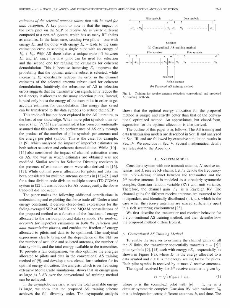
Fig. 1. Training for receive antenna selection: conventional and proposedAS training methods.

shows that the optimal energy allocation for the proposedmethod is unique and strictly better than that of the conven-tional optimized method. An approximate, but closed-form,expression for the optimal allocation is also derived.

The outline of this paper is as follows. The AS training anddata transmission models are described in Sec. II and analyzedin Sec. III, and are followed by extensive simulation results inSec. IV. We conclude in Sec. V. Several mathematical detailsare relegated to the Appendix.

II. SYSTEM MODEL

Consider a system with one transmit antenna, 𝑁 receive an-tennas, and 𝐿 receive RF chains. Let ℎ𝑘 denote the frequency-flat, block-fading channel between the transmitter and the𝑘th receive antenna. It is modeled as a circularly symmetriccomplex Gaussian random variable (RV) with unit variance.Therefore, the channel gain ∣ℎ𝑘∣ is a Rayleigh RV. Thechannel gains for different receive antennas are assumed to beindependent and identically distributed (i. i. d.), which is thecase when the receive antennas are spaced sufficiently apartin a rich scattering environment [23].

We first describe the transmitter and receiver behavior forthe conventional AS training method, and then describe howthe proposed method differs from it.

A. Conventional AS Training Method

To enable the receiver to estimate the channel gains of allthe 𝑁 links, the transmitter sequentially transmits 𝑎 = ⌈𝑁𝐿 ⌉pilot symbols [9], [15] each with energy 𝜀𝐸1, sequentially, asshown in Figure 1(a), where 𝐸1 is the energy allocated to adata symbol and 𝜀 ≥ 0 is the energy scaling factor for pilots.Each pilot symbol is received by at most 𝐿 receive antennas.

The signal received by the 𝑘th receive antenna is given by

𝑟𝑘 =√𝜀𝐸1𝑝ℎ𝑘 + 𝑛𝑘, (1)

where 𝑝 is the (complex) pilot with ∣𝑝∣ = 1, 𝑛𝑘 is acircular symmetric complex Gaussian RV with variance 𝑁0

that is independent across different antennas, 𝑘, and time. The


minimum mean square estimate (MMSE) channel estimate forthe 𝑘th antenna is [24]

ℎ̂𝑘 =

√𝜀𝐸1𝑝

∗

𝜀𝐸1 +𝑁0𝑟𝑘. (2)

Since the channel estimates of different antenna elementsare independent, the receiver selects the 𝐿 antennas with thehighest estimated channel gains. Let Ω̂𝐿 denote the selected

subset of antennas. Note that Ω̂𝐿 depends on{ℎ̂𝑘

}𝑁𝑘=1

.

The pilot symbols are followed by 𝑑 data symbols, eachtransmitted with energy 𝐸1. All the 𝑑 data symbols arereceived by the same antenna subset Ω̂𝐿. The received signalat the 𝑘th antenna for the 𝑙th data symbol, 𝑠(𝑙), equals

𝑦(𝑙)𝑘 = ℎ𝑘𝑠

(𝑙) + 𝑛(𝑙)𝑘 , 𝑘 ∈ Ω̂𝐿. (3)

The data symbols are equi-probable and derived from eitherthe MPSK or MQAM constellations. For MPSK, 𝑠(𝑙) ∈{√

𝐸1 exp(𝑗2𝜋𝑚𝑀 ),𝑚 = 0, . . . ,𝑀 − 1}. For MQAM, 𝑠(𝑙) =√

3𝐸1

2(𝑀−1) (𝑎𝐼 + 𝑗𝑎𝑄), where 𝑎𝐼 , 𝑎𝑄 ∈ {2𝑖 − 1 − √𝑀, 𝑖 =

1, . . . ,√𝑀}. To simplify the notation, we shall henceforth

drop the symbol index 𝑙, unless required otherwise.The maximum likelihood (ML) decision variable for decod-

ing a data symbol is 𝒟 =∑𝑘∈Ω̂𝐿

ℎ̂∗𝑘𝑦𝑘. The constraint on total

energy, 𝐸𝑇 , takes the form1

(𝑎𝜀+ 𝑑)𝐸1 = 𝐸𝑇 . (4)

Let 𝛾 ≜ 𝐸𝑇

𝑁0. Therefore, 𝐸1

𝑁0= 𝛾𝑎𝜀+𝑑 . Notice that the choice

of 𝜀 affects the energy allocated, 𝐸1, to each data symbol.

B. Proposed Method

We now describe the proposed AS training method, whichis shown in Figure 1(b). As before, the transmitter now firstsequentially transmits 𝑎 = ⌈𝑁𝐿 ⌉ pilot symbols so that all the𝑁channels can be estimated, with 𝐿 channels getting estimatedevery time a pilot is transmitted. But, each pilot symbol isnow transmitted with energy 𝛼𝐸2, where 𝐸2 is the energyper data symbol and 𝛼 is now the energy scaling factor forthese pilots.

The pilot symbol received by the 𝑘th receive antenna is𝑟𝑘 =

√𝛼𝐸2𝑝ℎ𝑘 + 𝑛𝑘, where 𝑛𝑘, as before, is a circular

symmetric complex Gaussian RV with variance 𝑁0. As in (2),the MMSE channel estimate for the 𝑘th antenna is given by

ℎ̂𝑘 =

√𝛼𝐸2𝑝

∗

𝛼𝐸2 +𝑁0𝑟𝑘 = 𝑎1ℎ𝑘 + 𝑒𝑘, (5)

where 𝑝 is the (complex) pilot with ∣𝑝∣ = 1, 𝑎1 ≜ 𝛼𝐸2

𝛼𝐸2+𝑁0,

and the zero-mean Gaussian noise term 𝑒𝑘 ≜ 𝑛𝑘𝑝∗√𝛼𝐸2

𝛼𝐸2+𝑁0has

a variance 𝜎2𝑒 =

𝛼𝐸2𝑁0

(𝛼𝐸2+𝑁0)2.

Since the channel estimates of different antennas are un-correlated, the 𝐿 antennas with the highest estimated channelgains are selected. As before, Ω̂𝐿 denotes the selected antenna

subset, and depends on{ℎ̂𝑘

}𝑁𝑘=1

.

1The case where the total pilot and data energy is less than 𝐸𝑇 issuboptimal, and is, therefore, not considered here.

Extra Pilot and Refined Estimates: The key difference in theproposed method is that an extra pilot symbol is transmittedwith energy 𝛽𝐸2, and is received by the selected 𝐿 antennas.The extra pilot helps in refining the channel estimates of theselected 𝐿 antennas as explained below. Note that, in general,𝛽 ∕= 𝛼. The received signal, 𝑟′𝑘, for the extra pilot is

𝑟′𝑘 =√𝛽𝐸2𝑝ℎ𝑘 + 𝑛′

𝑘, 𝑘 ∈ Ω̂𝐿, (6)

where 𝑛′𝑘 is a circular symmetric complex Gaussian RV with

variance 𝑁0, and is independent of 𝑛𝑘.The channel estimate of a selected antenna 𝑘 ∈ Ω̂𝐿 can

be refined using the two observations 𝑟′𝑘 and 𝑟𝑘 . The refined

MMSE estimate, ˆ̂ℎ𝑘, that uses both 𝑟𝑘 and 𝑟′𝑘 equals [24]

ˆ̂ℎ𝑘 =

√𝛼𝐸2𝑝

∗𝑟𝑘 +√𝛽𝐸2𝑝

∗𝑟′𝑘(𝛼+ 𝛽)𝐸2 +𝑁0

= 𝑎2ℎ𝑘 + 𝑒′𝑘, (7)

where 𝑎2 ≜ (𝛼+𝛽)𝐸2

(𝛼+𝛽)𝐸2+𝑁0and the zero-mean Gaussian noise

term 𝑒′𝑘 ≜√𝛼𝐸2𝑝

∗𝑛𝑘+√𝛽𝐸2𝑝

∗𝑛′𝑘

(𝛼+𝛽)𝐸2+𝑁0has a variance of 𝜎2

𝑒′ =(𝛼+𝛽)𝐸2𝑁0

((𝛼+𝛽)𝐸2+𝑁0)2. Note that 𝑒′𝑘 and 𝑒𝑘 are correlated.

Data Reception: The pilot symbols are followed by 𝑑data symbols, each transmitted with energy 𝐸2. They are allreceived by the antenna subset Ω̂𝐿.2 The received signal fora data symbol 𝑠 is

𝑦𝑘 = ℎ𝑘𝑠+ 𝑛′′𝑘, 𝑘 ∈ Ω̂𝐿. (8)

The maximum likelihood decision variable, 𝒟, for data de-coding is 𝒟 =

∑𝑘∈Ω̂𝐿

ˆ̂ℎ∗𝑘𝑦𝑘. The total energy constraint is

𝐸𝑇 = (𝑎𝛼+ 𝛽 + 𝑑)𝐸2. (9)

Let 𝛾 ≜ 𝐸𝑇

𝑁0. Hence, 𝐸2

𝑁0= 𝛾𝑎𝛼+𝛽+𝑑 . Now, 𝛼 and 𝛽 together

affect the energy 𝐸2 allocated to a data symbol. When 𝛽 = 0,the SEP of the proposed method is the same as that of theconventional AS training method with 𝜀 = 𝛼.

While a corresponding scheme can be developed for multi-ple transmit antennas, its analysis is beyond the scope of thispaper. Even the one transmit antenna case considered in thispaper will turn out to be analytically interesting and insightful.

III. SEP ANALYSIS AND OPTIMIZATION

We now analyze the fading-averaged SEP for MPSK orMQAM for receive AS with imperfect CSI for the conven-tional and proposed AS training methods, and optimize theirparameters to minimize the SEP. The case where channelcoding is used across the 𝑑 symbols is beyond the scope of thispaper due to its analytical intractability. This approach has alsobeen followed in [6], [9], [12], [17], which focus on the SEP togain insights. While [25] did analyze AS with channel coding,channel estimation errors or training details for AS were notaddressed. Henceforth, E [𝐴] and var [𝐴] shall denote theexpectation and variance, respectively, of RV 𝐴. E [𝐴∣𝐵] andvar [𝐴∣𝐵] will denote the conditional expectation and varianceof 𝐴 given 𝐵, respectively; 𝑥∗ denotes the complex conjugateof scalar 𝑥; 𝑌 𝐻 denotes the Hermitian transpose of vector 𝑌 .

2After receiving the extra pilot, the receiver can, in fact, reselect the

antennas based on ℎ̂𝑘 or ˆ̂ℎ𝑘, depending on whether 𝑘 is in Ω̂𝐿 or not. We

do not allow this to keep the analysis tractable. Simulations show that theperformance gains from such a reselection are negligible.


A. Conventional Method Optimization

We discuss the conventional method only briefly given theanalysis in [9]. The main contribution of this section liesin determining the optimal value of 𝜀 that minimizes theSEP subject to total energy constraint, and in deriving theexpression for the optimal SEP; these were are not consideredin [9]. This provides a fair benchmark for our new method,which is analyzed next.

In terms of the notation used in our paper, the SEP ex-pressions for MPSK and MQAM, denoted by 𝑃 𝜀MPSK(𝛾) and𝑃 𝜀MQAM(𝛾), respectively, are [9]:

𝑃 𝜀MPSK(𝛾) =1

𝜋

∫ 𝑀−1𝑀 𝜋

0

(sin2 𝜃

sin2 𝜃 + 𝑐PSK

)𝐿

×𝑁∏

𝑛=𝐿+1

(sin2 𝜃

sin2 𝜃 + 𝑐PSK𝐿𝑛

)𝑑𝜃, (10)

𝑃 𝜀MQAM(𝛾) =4

𝜋

(1− 1√

𝑀

)∫ 𝜋2

0

𝜉(𝜃)

(sin2 𝜃

sin2 𝜃 + 𝑐QAM

)𝐿

×𝑁∏

𝑛=𝐿+1

(sin2 𝜃

sin2 𝜃 + 𝑐QAM𝐿𝑛

)𝑑𝜃, (11)

where 𝜉(𝜃) = 1√𝑀

, for 0 ≤ 𝜃 < 𝜋4 , and 𝜉(𝜃) = 1, for

𝜋4 ≤ 𝜃 ≤ 𝜋

2 ; 𝑐PSK ≜ 𝜀𝛾2 sin2( 𝜋𝑀 )

(𝑎𝜀+𝑑)((𝜀+1)𝛾+𝑎𝜀+𝑑) , and 𝑐QAM ≜1.5𝜀𝛾2/(𝑀−1)

(𝑎𝜀+𝑑)((𝜀+1)𝛾+𝑎𝜀+𝑑) .Lemma 1: The optimal value of 𝜀, denoted by 𝜀∗(𝛾), that

minimizes the SEP of both MPSK and MQAM is

𝜀∗(𝛾) =

√𝑑(𝛾 + 𝑑)

𝑎(𝛾 + 𝑎). (12)

Proof: The proof is given in Appendix A.

When 𝛾 → ∞, we have lim𝛾→∞𝜀

∗(𝛾) ≜ 𝜀∗∞ =√𝑑𝑎 . Note

that this asymptotic result (but not the general expressionfor any 𝛾 in Lemma 1) can also be construed as a specialcase of the result in [22, (15)], which considered energyallocation between data symbols and mid-amble pilots in aTD-CDMA system to minimize mean square estimation error.Consequently, the asymptotic expression for the optimal SEPof MPSK, 𝑃 𝜀,∞MPSK(𝛾), simplifies to

𝑃 𝜀,∞MPSK (𝛾) = 𝛾−𝑁(𝐿+ 1) (𝐿+ 2) ⋅ ⋅ ⋅ (𝑁)

𝜋4𝑁𝐿𝑁−𝐿(√

𝑑+√𝑎)2𝑁

× sin−2𝑁( 𝜋𝑀

)𝜓

(𝑀 − 1𝑀

𝜋,𝑁

), (13)

where 𝜓 (𝑇,𝑁) ≜(2𝑁𝑁

)𝑇+

𝑁−1∑𝑗=0

(−1)𝑗+𝑁

𝑁−𝑗(2𝑁𝑗

)sin(2(𝑁−𝑗)𝑇 ).

The derivation is relegated to Appendix B. The asymptoticexpression for the optimal SEP of MQAM can be writtensimilarly.

B. Analysis and Optimization of SEP of Proposed Method

We now analyze the SEP of the proposed method given 𝛼and 𝛽, and then minimize it. The following result about thestatistics of 𝒟 shall be useful in deriving the SEP.

Lemma 2: Conditioned on{ℎ̂𝑙,ˆ̂ℎ𝑙

}𝑙∈Ω̂𝐿

and 𝑠, the deci-

sion variable, 𝒟, is a complex Gaussian RV with conditionalmean, 𝜇𝒟 , and variance, 𝜎2

𝒟 , given by

𝜇𝒟 ≜ E

[𝒟⏐⏐⏐{ℎ̂𝑙, ˆ̂ℎ𝑙}

𝑙∈Ω̂𝐿

, 𝑠

]= 𝑠

∑𝑘∈Ω̂𝐿

∣∣∣ˆ̂ℎ𝑘∣∣∣2 , (14)

𝜎2𝒟≜var

[𝒟⏐⏐⏐{ℎ̂𝑙, ˆ̂ℎ𝑙}

𝑙∈Ω̂𝐿

, 𝑠

]= ((1−𝑎2)𝐸2+𝑁0)

∑𝑘∈Ω̂𝐿

∣∣∣ˆ̂ℎ𝑘∣∣∣2.(15)

Proof: The proof is given in Appendix C.

Since 𝜇𝒟 and 𝜎2𝒟 depend only on ˆ̂ℎ𝑘, we see that all the

information in ℎ̂𝑘 is captured by ˆ̂ℎ𝑘. We now derive the SEPfor MPSK and MQAM for the proposed method as a functionof 𝛼 and 𝛽.

Theorem 1: With noisy channel estimates, the fading-averaged SEP of MPSK and MQAM is:

𝑃𝛼,𝛽MPSK(𝛾) =1

𝜋

∫ 𝑀−1𝑀 𝜋

0

(sin2 𝜃

𝑎2𝑏PSK + sin2 𝜃

)𝐿

×𝑁∏

𝑛=𝐿+1

(1 +

𝑎1𝑏PSK𝐿/𝑛

(𝑎2 − 𝑎1)𝑏PSK + sin2 𝜃

)−1

𝑑𝜃, (16)

𝑃𝛼,𝛽MQAM(𝛾)=4

𝜋

(1− 1√

𝑀

)∫ 𝜋2

0

𝜉(𝜃)

(sin2 𝜃

𝑎2𝑏QAM+sin2 𝜃

)𝐿

×𝑁∏

𝑛=𝐿+1

(1+

𝑎1𝑏QAM𝐿/𝑛

(𝑎2−𝑎1)𝑏QAM+sin2 𝜃

)−1

𝑑𝜃, (17)


, for 0 ≤ 𝜃 < 𝜋4 , and 𝜉(𝜃) = 1, for 𝜋4 ≤

𝜃 ≤ 𝜋2 , 𝑎1 =

𝛼𝛾(𝑎+𝛾)𝛼+𝛽+𝑑 , 𝑎2 =

(𝛼+𝛽)𝛾(𝑎+𝛾)𝛼+(𝛾+1)𝛽+𝑑 , 𝑏PSK =

𝛾 sin2( 𝜋𝑀 )

(1−𝑎2)𝛾+𝑎𝛼+𝛽+𝑑 , and 𝑏QAM =1.5𝛾/(𝑀−1)

(1−𝑎2)𝛾+𝑎𝛼+𝛽+𝑑 .Proof: The proof is given in Appendix D.

Closed-form expressions can be derived from (16) and (17)using [26, (5A.42), (5A.56)]. However, they are quite involved,and are not shown here. The optimal values of 𝛼 and 𝛽 arethen found numerically using gradient search. Considerableinsight about them can be gained by analyzing the asymptoticenergy regime, as we show below.

C. Asymptotic Characterization of SEP (𝛾 → ∞)

In the asymptotic regime, the SEP of MPSK and MQAMshall be denoted by 𝑃𝛼,𝛽,∞MPSK (𝛾) and 𝑃𝛼,𝛽,∞MQAM (𝛾), respectively.In the results below, we do not show higher order termsinvolving 𝛾 since their contribution becomes negligible as𝛾 → ∞.

Lemma 3: The asymptotic SEPs of MPSK and MQAMare given by

𝑃𝛼,𝛽,∞MPSK (𝛾) = 𝛾−𝑁(𝐿+ 1) (𝐿+ 2) ⋅ ⋅ ⋅ (𝑁)𝜋𝐿𝑁−𝐿 (4(𝛼+ 𝛽))

𝑁

× (𝑎𝛼+ 𝛽 + 𝑑)𝑁(𝛼+ 𝛽 + 1)

𝑁sin−2𝑁

( 𝜋𝑀

)

×𝑁−𝐿∑𝑘=0

(𝑁−𝐿𝑘

)(4𝛽 sin2

(𝜋𝑀

)𝛼(𝛼+𝛽+1)

)𝑘𝜓

(𝑀−1𝑀

𝜋,𝑁−𝑘), (18)


𝑃𝛼,𝛽,∞MQAM (𝛾) = 𝛾−𝑁4 (𝐿+1) (𝐿+2) ⋅ ⋅ ⋅ (𝑁)𝜋𝐿𝑁−𝐿 (6(𝛼+ 𝛽))

𝑁

× (𝑎𝛼+ 𝛽 + 𝑑)𝑁(𝛼+ 𝛽 + 1)

𝑁(𝑀 − 1)𝑁

(1− 1√

𝑀

)

×𝑁−𝐿∑𝑘=0

[(𝑁 − 𝐿

𝑘

)(6𝛽/(𝑀 − 1)𝛼(𝛼+ 𝛽 + 1)

)𝑘

×(𝜓(𝜋2, 𝑁 − 𝑘

)−(1− 1√

𝑀

)𝜓(𝜋4, 𝑁 − 𝑘

))].

(19)

Proof: The proof is given in Appendix E.The above expressions show that the diversity order is 𝑁 forany 𝛼 > 0 and 𝛽 ≥ 0. This is to be expected since theconventional training method, which is a special case of theproposed scheme with regard to SEP, also achieves a diversityorder of 𝑁 .

Even the form in (18) is intractable for determining theoptimal values of 𝛼 and 𝛽. We, therefore, minimize an upperbound on the SEP that is obtained by replacing sin2 𝜃 with 1in (16) [27]. Let 𝛼∗

∞ and 𝛽∗∞ denote the optimal values of 𝛼

and 𝛽, respectively, that minimize the SEP upper bound.From the proof of Lemma 3 in Appendix E (see (41)), it

can be shown that 𝑃𝛼,𝛽,∞MPSK (𝛾) ≤ 𝛾−𝑁𝑈𝛼,𝛽MPSK (𝛾), where

𝑈𝛼,𝛽MPSK ≜ (𝐿+1) (𝐿+2) ⋅ ⋅ ⋅ (𝑁)𝐿𝑁−𝐿

(𝑀−1𝑀

)sin−2𝑁

( 𝜋𝑀

)

×((𝑎𝛼+𝛽+𝑑)(𝛼+𝛽+1)

𝛼+𝛽

)𝑁(1+

𝛽 sin2(𝜋𝑀

)𝛼(𝛼+𝛽+1)

)𝑁−𝐿. (20)

Similarly, for MQAM, 𝑃𝛼,𝛽,∞MQAM (𝛾) ≤ 𝛾−𝑁𝑈𝛼,𝛽MQAM, where

𝑈𝛼,𝛽MQAM ≜ (𝐿+1) (𝐿+2) ⋅ ⋅ ⋅ (𝑁)𝐿𝑁−𝐿

(𝑀−1𝑀

)(1.5

𝑀−1)−𝑁

×((𝑎𝛼+𝛽+𝑑)(𝛼+𝛽+1)

𝛼+𝛽

)𝑁 ⎛⎝1+ 𝛽(

1.5𝑀−1

)𝛼(𝛼+𝛽+1)

⎞⎠𝑁−𝐿

. (21)

As we see below, the upper bounds provide considerableinsight about the optimal parameters. Specifically, for MPSK,𝛼∗∞ and 𝛽∗

∞ satisfy the following properties:Theorem 2: 1) 𝛼∗

∞ and 𝛽∗∞ are related by

𝛽∗∞ = −𝛼∗

∞ +

√𝑑− (𝛼∗∞)

2(𝑎− 1). (22)

2) 𝛼∗∞ is a zero of the function 𝑔1(𝛼), where

𝑔1(𝛼)≜√𝑑−𝛼2(𝑎−1)

(𝑁𝛼2csc2

( 𝜋𝑀

)+ 𝐿𝛼−𝑑

(𝑁−𝐿𝑎−1

))

+ 𝛼2(𝑁 csc2

( 𝜋𝑀

)− 𝐿)− 𝑑

(𝑁 − 𝐿

𝑎− 1). (23)

3) And, 𝛼∗∞ is unique and lies in the following range:

0 < 𝛼∗∞ ≤

√𝑑(𝑁 − 𝐿)

𝑁(𝑎− 1) sin( 𝜋𝑀

)≤ 𝜀∗∞ =

√𝑑

𝑎, (24)

with the equalities holding only if both the following condi-tions hold: 𝑀 = 2 (BPSK) and 𝐿 divides 𝑁 .

Proof: The proof is given in Appendix F.

For large constellation sizes (𝑀 → ∞), the optimal values𝛼∗∞ and 𝛽∗

∞ can, in fact, be determined in closed-form asshown below.

Corollary 1:

lim𝑀→∞

𝛼∗∞sin(𝜋𝑀

) =√𝑑(𝑁 − 𝐿)

𝑁(𝑎− 1) . (25)

Proof: The proof is given in Appendix G.Corollary 1 motivates the following approximation for any

𝑀 , which is obtained by substituting (25) in (22):

𝛼∗∞≈

√𝑑(𝑁−𝐿)𝑁(𝑎−1) sin

( 𝜋𝑀

), (26)

𝛽∗∞≈ −


( 𝜋𝑀

)+√𝑑

√1−(1− 𝐿

𝑁

)sin2

( 𝜋𝑀

).

(27)

From the Corollary, it directly follows that the error in theapproximation disappears as 𝑀 → ∞. Interestingly, we shallsee that the error in (26) is small even when 𝑀 is as smallas 4.

Corresponding Results for MQAM: Results analogous toTheorem 2 and Corollary 1 are obtained for MQAM by

simply replacing sin(𝜋𝑀

)with

√1.5𝑀−1 . This follows because

the expressions in (20) and (21) are very similar except that

sin(𝜋𝑀

)is replaced by

√1.5𝑀−1 .

The asymptotic expressions for SEP provide the followinginsights about the proposed scheme.

1) Variation with System Parameters: While 𝜀∗∞ in theconventional method depends only on 𝑑 and the number ofpilot symbols, 𝑎; in the proposed scheme, 𝛼∗

∞ depends onall system parameters 𝑁 , 𝐿, 𝑑, 𝑀 , and 𝑎. Furthermore, as 𝑑increases, the relative energy allocated to training increasesin the conventional and proposed methods. This trend isconsistent with the observations in [18], which consideredtraining for multiple antenna systems to maximize averagethroughput.

2) BPSK (𝑀 = 2): Theorem 2 shows that this is the onlycase when the proposed method provides no benefits over theconventional method if 𝐿 divides 𝑁 . As expected, for thiscase, (24) implies that 𝛼∗

∞ = 𝜀∗∞ and 𝛽∗∞ = 0. However,

the conclusion is different when 𝐿 does not divide 𝑁 evenfor BPSK. In this case, 𝛼∗

∞ < 𝜀∗∞, and the proposed schemenecessarily improves performance.

3) Asymptotic Energy Gain: The conventional and pro-posed methods both achieve the full diversity order of 𝑁 .Hence, we can compare them in terms of the asymptoticenergy gain, Δ, which measures the savings in total energyachieved by the proposed method over the conventional op-timized method for the same SEP. It is easy to see that, forMPSK, Δ = 10

𝑁 log10

(𝑃 𝜀,∞MPSK/𝑃

𝛼,𝛽,∞MPSK

)dB.

Taking the ratio of (13) and (18), we get

Δ = 10 log10

⎛⎜⎝

(√𝑑+

√𝑎)2(𝛼∗

∞ + 𝛽∗∞)

(𝛼∗∞ + 𝛽∗∞ + 1) (𝑎𝛼∗∞ + 𝛽∗∞ + 𝑑)

⎞⎟⎠


− 10

𝑁log10

[𝑁−𝐿∑𝑘=0

(𝑁−𝐿𝑘

)(4𝛽∗

∞ sin2(𝜋𝑀

)𝛼∗∞ (𝛼∗∞ + 𝛽∗∞ + 1)

)𝑘

×(𝜓

(𝑀−1𝑀

𝜋,𝑁−𝑘)/

𝜓

(𝑀 − 1𝑀

𝜋,𝑁

))], (28)

where 𝛼∗∞ and 𝛽∗

∞ are either found numerically or approxi-mated using (26).

4) Energy Allocation: 𝐸1 ≤ 𝐸2 and 𝛼∗∞ + 𝛽∗

∞ ≥ 𝜀∗∞.From (4) and (9), for optimal values of the parameters, it can

be seen that 𝐸1

𝐸2− 1 = (𝑎−1)𝛼∗

∞+√𝑑−(𝛼∗∞)2(𝑎−1)−𝑎𝜀∗∞𝑎𝜀∗∞+𝑑 . This is

negative because 𝑑−(𝛼∗∞)

2(𝑎−1)−(𝑎𝜀∗∞ − (𝑎− 1)𝛼∗

∞)2=

−𝑎(𝑎 − 1) (𝜀∗∞ − 𝛼∗∞)

2 ≤ 0 (since 𝑎 ≥ 1). Thus, 𝐸1 ≤ 𝐸2.

From (26), 𝛼∗∞+𝛽∗

∞𝜀∗∞

=√𝑎√1− (1− 𝐿

𝑁

)sin2

(𝜋𝑀

). Since

𝑎 ≥ 𝑁𝐿 , it follows that (𝛼∗

∞ + 𝛽∗∞)/𝜀

∗∞ ≥ 1. Furthermore,

the ratio increases as 𝑀 increases.Note that 𝜀∗∞𝐸1 and (𝛼∗

∞ + 𝛽∗∞)𝐸2 respectively denote

the quality of channel estimates used for data decoding inthe conventional method and the proposed method. Thus, theproposed method not only allocates more energy to each datasymbol (since 𝐸2 ≥ 𝐸1), but it also ensures that the qualityof estimates is better than the conventional method (since(𝛼∗∞ + 𝛽∗∞)𝐸2 ≥ 𝜀∗∞𝐸1).

5) Behavior of 𝐸2/𝐸1, i.e., Ratio of Data Energies Allo-cated by The Two Methods: Understanding the behavior of𝐸2/𝐸1 will help explain the behavior of SEP and Δ in thenext section.

(i) 𝐸2/𝐸1 increases with 𝑀 : To show this, it is sufficient toshow that ∂

∂𝛼∗∞𝐸2

𝐸1≤ 0 since 𝛼∗∞ scales as sin

(𝜋𝑀

). From (4)

and (9), it can be seen that 𝐸2

𝐸1=

𝑎𝜀∗∞+𝑑

(𝑎−1)𝛼∗∞+√𝑑−(𝛼∗∞)2(𝑎−1)+𝑑

.

Since 𝜀∗∞ does not depend on 𝑀 , its sufficient to showthat the denominator is non-decreasing in 𝛼∗

∞. This follows

because ∂∂𝛼∗∞

((𝑎− 1)𝛼∗

∞ +

√𝑑− (𝛼∗∞)

2(𝑎− 1)

)= (𝑎 −

1)

(1− 𝛼∗

∞√𝑑−(𝛼∗∞)2(𝑎−1)

)≥ 0 since 𝛼∗

∞ ≤√𝑑𝑎 .

(ii) 𝐸2/𝐸1 increases with 𝐿 and decreases with 𝑁 (when𝑎 is fixed): From (4), (9), and Theorem 2, we see that 𝐸2

𝐸1=

𝑎𝜀∗∞+𝑑

(𝑎−1)𝛼∗∞+√𝑑−(𝛼∗∞)2(𝑎−1)+𝑑

. Substituting the optimal values

of the parameters and simplifying further, we get

𝐸2

𝐸1=

√𝑎+

√𝑑√

(𝑎− 1)𝜏 +√1− 𝜏 +

√𝑑, (29)

where 𝜏 ≜(1− 𝐿

𝑁

)sin2

(𝜋𝑀

). To prove the desired result it

is sufficient to show that the denominator is non-decreasingin 𝜏 . This follows because

∂

∂𝜏(√(𝑎− 1)𝜏 +√

1− 𝜏 ) = 0.5

(√𝑎− 1𝜏

−√

1

1− 𝜏

).

This is non-negative because the inequality 𝑎 ≥ 𝑁𝐿 implies that(

1− 1𝑎

) ≥ 𝜏 , which after algebraic manipulations implies that√𝑎−1𝜏 ≥

√1

1−𝜏 .(iii) 𝐸2/𝐸1 decreases with 𝑑: On substituting the optimal

values of parameters, the expression for the ratio simplifiesto 𝐸2

𝐸1=

√𝑎+

√𝑑√

(𝑎−1)(1− 𝐿𝑁 ) sin(

𝜋𝑀 )+

√1−(1− 𝐿

𝑁 ) sin2( 𝜋𝑀 )+

√𝑑. Since

0 5 10 15 20

10−2

10−1

100

ET/dN

0 = γ/d (dB)

Ave

rage

SE

P (γ

)

Conventional methodProposed methodSimulationGradient search

M = 16

M = 8

M = 4

Fig. 2. Effect of constellation size on average SEP of MPSK (𝑁 = 6,𝐿 = 1, and 𝑑 = 10).

0 5 10 15 20

10−2

10−1

100

ET/dN

0 = γ/d (dB)

Ave

rage

SE

P (γ

)

Conventional methodProposed methodSimulationGradient search

M = 16

M = 4

Fig. 3. Effect of constellation size on average SEP of MQAM (𝑁 = 6,𝐿 = 1, and 𝑑 = 10).

𝐸2 ≥ 𝐸1, as shown in Sec. III-C4, the expression takes theform 𝐸2

𝐸1= 1 + 𝑓1

𝑓2, with 𝑓1 is positive and independent of 𝑑,

and 𝑓2 is positive and monotonically increases with 𝑑. Hence,the ratio decreases with 𝑑.

IV. SIMULATION RESULTS

We now plot the analytical results derived in Sec. III andvalidate them with Monte Carlo simulations that use 105

samples for each SNR. As specified in the system model, thechannel remains constant for 𝑑 + 𝑎 + 1 symbols. We alsocompare the conventional and proposed AS training methodsas a function of all the system parameters 𝑁 , 𝐿, 𝑑, and 𝑀 .

Figures 2 and 3 plot the SEP as a function of normalizedtotal energy, 𝐸𝑇

𝑑𝑁0(= 𝛾

𝑑 ), for MPSK and MQAM, respectively,for a given 𝐿 and 𝑁 . While the SEP of both methodsexpectedly increases with 𝑀 , the performance gain of theproposed method increases with 𝑀 . This is because 𝜀∗∞ of theconventional method is insensitive to 𝑀 despite the fact that


−10 −5 0 5 10 15 200

0.5

1

1.5

2

2.5

3

3.5

ET/dN

0 = γ/d (dB)

Par

amet

er V

alue

(γ)

α∗(γ)

β∗(γ)

ε∗(γ)

ε∞∗

β∞∗

α∞∗

Fig. 4. Optimal values of different parameters as a function of 𝐸𝑇𝑑𝑁0

(8PSK,𝑁 = 6, 𝐿 = 1, and 𝑑 = 10).

the SEP of larger constellations is more sensitive to channelestimation errors. The optimal values of 𝛼 and 𝛽 that areused in the figures are found by using a gradient search overthe SEP formulae of Theorem 1.3 The figures also plot theSEP obtained by using the approximate values of 𝛼∗∞ and 𝛽∗∞given in (26). Notice that the SEP using the approximation isaccurate even at low values of 𝛾. Furthermore, there is anexcellent match between the analytical and simulation results.The small mismatch between analytical and simulation resultsfor MQAM is explained in Appendix D.

Figure 4 shows the optimal energy allocation (𝜀∗, 𝛼∗, and𝛽∗) as a function of the normalized total energy. 𝛼∗(𝛾) and𝛽∗(𝛾) are obtained by performing a gradient search that min-imizes 𝑃𝛼−𝛽MPSK(𝛾). Also shown are the asymptotically optimalvalues 𝛼∗

∞ and 𝛽∗∞ of (26). These are very close to the exact

optimal values for 𝛾𝑑 ≥ 15 dB. Henceforth, we, therefore,

only use 𝛼∗∞ and 𝛽∗

∞ of (26), unless mentioned otherwise. Inthe conventional method, 𝜀∗ monotonically decreases with 𝛾

and saturates at√𝑑𝑎 = 1.291. However, the proposed method

behaves differently. At low 𝛾, 𝛼∗(𝛾) is close to zero and 𝛽∗(𝛾)is large since selection does not matter, only coherent receptiondoes. Once 𝛾 crosses a threshold, the system allocates moreenergy to the selection pilots. This triggers a correspondingdecrease in 𝛽∗(𝛾) since the selection pilot and the last pilotare both used for coherent reception.

Figure 5 shows the effect of the antenna subset size, 𝐿, onthe SEP. As 𝐿 increases, the number of pilots that need to betransmitted decreases. Hence, relatively less energy is spent ontraining. Consequently, for both methods, the SEP improvesfor all 𝛾.4

3Since the optimal solution is unique in the asymptotic regime (𝛾 → ∞),we know that the gradient search will converge to the global minimum atleast for large 𝛾. In our numerical computations, we have observed the samefor smaller 𝛾, as well.

4The behavior with 𝑁 turns out to be different. At low 𝛾, a smaller 𝑁 isbetter because the energy-starved system cannot afford to spend energy ontraining. At high 𝛾, where diversity order matters, a larger 𝑁 does better.Due to the better utilization of energy by the proposed method, this crossoverturns out to occur at a smaller value of 𝛾.

0 5 10 15 20

10−2

10−1

100

ET/dN

0 = γ/d (dB)

Ave

rage

SE

P (γ

)

Conventional methodProposed methodSimulation

L = 1

L = 2

L = 3

L = 6

Fig. 5. Effect of number of receive RF chains on average SEP (8PSK,𝑁 = 6, and 𝑑 = 10).

1 2 3 4 5 6 7 8 9 100

0.5

1

1.5

2

2.5

3

N (Number of receive antennas)

Asy

mpt

otic

Ene

rgy

Gai

n (d

B)

Gradient searchAsymptotic approximation

M = 16

M = 8

M = 4

M = 2

Fig. 6. Effect of number of receive antennas on asymptotic energy gain(MPSK, 𝑑 = 10, and 𝐿 = 1).

Figure 6 plots the asymptotic energy gain, Δ, as a functionof 𝑁 and 𝑀 . We can see that the energy gain increaseswith 𝑀 . This is because: (i) The relative quality of estimatesimproves with 𝑀 . (This can be seen from the behavior of theratio 𝛼∗

∞+𝛽∗∞

𝜀∗∞, which was discussed in Sec. III-C4.) (ii) The

proposed method allocates relatively more energy to the datasymbols, as shown in Sec. III-C5. A similar argument, notrepeated here due to space constraints, also explains thevariation with 𝑁 .

Figure 7 plots the energy gain as a function of 𝐿 for fixed𝑁 and different values of 𝑀 . We choose 𝑁 as 16 in order toillustrate how the energy gain increases as 𝐿 increases from𝑁2 to 𝑁 − 1. This figure can be understood as follows: (i) For𝑁2 ≤ 𝐿 < 𝑁 , 𝑎 is fixed at 2. Hence, 𝛼

∗∞+𝛽∗

∞𝜀∗∞

increases with 𝐿.(ii) 𝐸2/𝐸1 increases with 𝐿, as shown in Sec. III-C5. Hence,the energy gain increases with 𝐿 in this region. The same istrue even when 𝐿 increases from 4 to 5 (𝑎 = 4) and 6 to 7(𝑎 = 3). In other regions, as 𝐿 increases, 𝑎 decreases. Hence,the energy gain decreases.

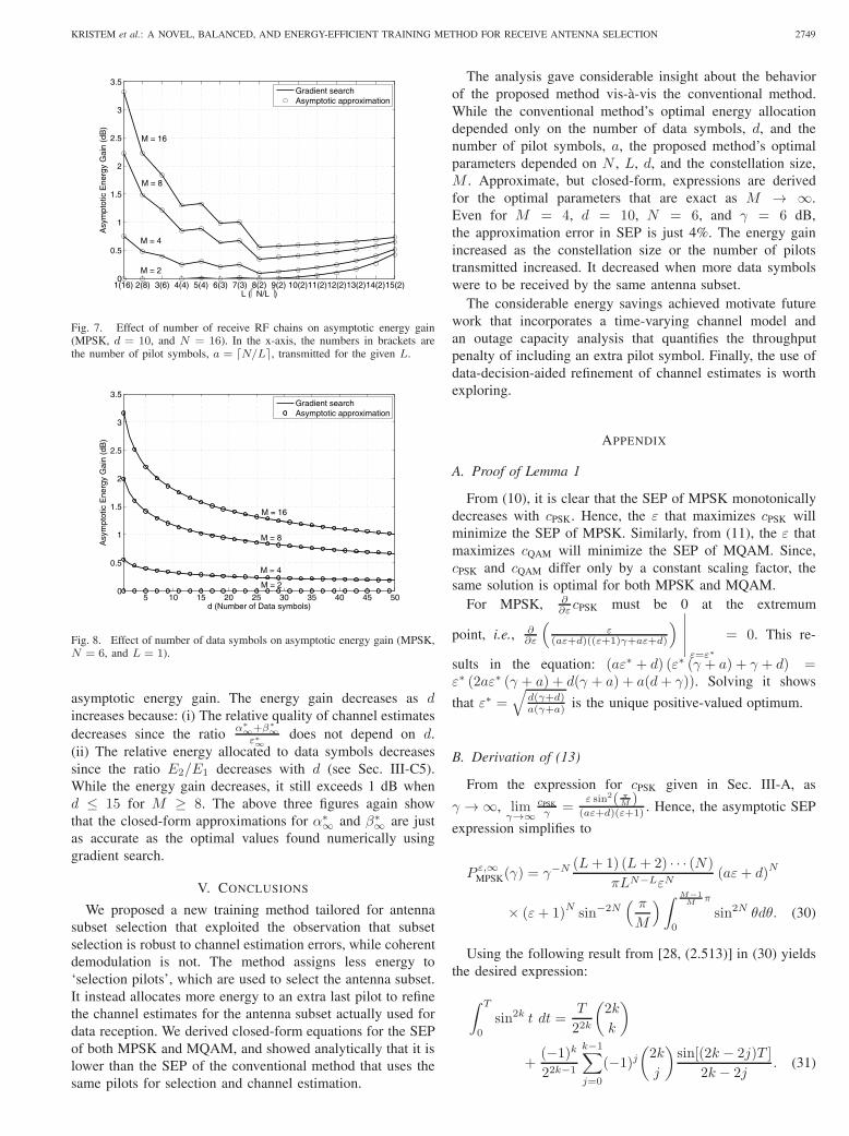
Figure 8 studies the joint impact of 𝑑 and 𝑀 on the


1(16) 2(8) 3(6) 4(4) 5(4) 6(3) 7(3) 8(2) 9(2) 10(2)11(2)12(2)13(2)14(2)15(2)0

0.5

1

1.5

2

2.5

3

3.5

L (⎡ N/L ⎤)

Asy

mpt

otic

Ene

rgy

Gai

n (d

B)


M = 16

M = 8

M = 4

M = 2

Fig. 7. Effect of number of receive RF chains on asymptotic energy gain(MPSK, 𝑑 = 10, and 𝑁 = 16). In the x-axis, the numbers in brackets arethe number of pilot symbols, 𝑎 = ⌈𝑁/𝐿⌉, transmitted for the given 𝐿.

5 10 15 20 25 30 35 40 45 500

0.5

1

1.5

2

2.5

3

3.5

d (Number of Data symbols)

Asy

mpt

otic

Ene

rgy

Gai

n (d

B)


M = 16

M = 8

M = 4

M = 2

Fig. 8. Effect of number of data symbols on asymptotic energy gain (MPSK,𝑁 = 6, and 𝐿 = 1).

asymptotic energy gain. The energy gain decreases as 𝑑increases because: (i) The relative quality of channel estimatesdecreases since the ratio 𝛼∗

∞+𝛽∗∞

𝜀∗∞does not depend on 𝑑.

(ii) The relative energy allocated to data symbols decreasessince the ratio 𝐸2/𝐸1 decreases with 𝑑 (see Sec. III-C5).While the energy gain decreases, it still exceeds 1 dB when𝑑 ≤ 15 for 𝑀 ≥ 8. The above three figures again showthat the closed-form approximations for 𝛼∗∞ and 𝛽∗∞ are justas accurate as the optimal values found numerically usinggradient search.

V. CONCLUSIONS

We proposed a new training method tailored for antennasubset selection that exploited the observation that subsetselection is robust to channel estimation errors, while coherentdemodulation is not. The method assigns less energy to‘selection pilots’, which are used to select the antenna subset.It instead allocates more energy to an extra last pilot to refinethe channel estimates for the antenna subset actually used fordata reception. We derived closed-form equations for the SEPof both MPSK and MQAM, and showed analytically that it islower than the SEP of the conventional method that uses thesame pilots for selection and channel estimation.

The analysis gave considerable insight about the behaviorof the proposed method vis-à-vis the conventional method.While the conventional method’s optimal energy allocationdepended only on the number of data symbols, 𝑑, and thenumber of pilot symbols, 𝑎, the proposed method’s optimalparameters depended on 𝑁 , 𝐿, 𝑑, and the constellation size,𝑀 . Approximate, but closed-form, expressions are derivedfor the optimal parameters that are exact as 𝑀 → ∞.Even for 𝑀 = 4, 𝑑 = 10, 𝑁 = 6, and 𝛾 = 6 dB,the approximation error in SEP is just 4%. The energy gainincreased as the constellation size or the number of pilotstransmitted increased. It decreased when more data symbolswere to be received by the same antenna subset.

The considerable energy savings achieved motivate futurework that incorporates a time-varying channel model andan outage capacity analysis that quantifies the throughputpenalty of including an extra pilot symbol. Finally, the use ofdata-decision-aided refinement of channel estimates is worthexploring.

APPENDIX

A. Proof of Lemma 1

From (10), it is clear that the SEP of MPSK monotonicallydecreases with 𝑐PSK. Hence, the 𝜀 that maximizes 𝑐PSK willminimize the SEP of MPSK. Similarly, from (11), the 𝜀 thatmaximizes 𝑐QAM will minimize the SEP of MQAM. Since,𝑐PSK and 𝑐QAM differ only by a constant scaling factor, thesame solution is optimal for both MPSK and MQAM.

For MPSK, ∂∂𝜀𝑐PSK must be 0 at the extremum

point, i.e., ∂∂𝜀

(𝜀

(𝑎𝜀+𝑑)((𝜀+1)𝛾+𝑎𝜀+𝑑)

)⏐⏐⏐⏐⏐𝜀=𝜀∗

= 0. This re-

sults in the equation: (𝑎𝜀∗ + 𝑑) (𝜀∗ (𝛾 + 𝑎) + 𝛾 + 𝑑) =𝜀∗ (2𝑎𝜀∗ (𝛾 + 𝑎) + 𝑑(𝛾 + 𝑎) + 𝑎(𝑑+ 𝛾)). Solving it shows

that 𝜀∗ =√𝑑(𝛾+𝑑)𝑎(𝛾+𝑎) is the unique positive-valued optimum.

B. Derivation of (13)

From the expression for 𝑐PSK given in Sec. III-A, as

𝛾 → ∞, lim𝛾→∞

𝑐PSK𝛾 =

𝜀 sin2( 𝜋𝑀 )

(𝑎𝜀+𝑑)(𝜀+1) . Hence, the asymptotic SEP

expression simplifies to

𝑃 𝜀,∞MPSK(𝛾) = 𝛾−𝑁(𝐿+ 1) (𝐿+ 2) ⋅ ⋅ ⋅ (𝑁)

𝜋𝐿𝑁−𝐿𝜀𝑁(𝑎𝜀+ 𝑑)𝑁

× (𝜀+ 1)𝑁 sin−2𝑁( 𝜋𝑀

)∫ 𝑀−1𝑀 𝜋

0

sin2𝑁 𝜃𝑑𝜃. (30)

Using the following result from [28, (2.513)] in (30) yieldsthe desired expression:

∫ 𝑇0

sin2𝑘 𝑡 𝑑𝑡 =𝑇

22𝑘

(2𝑘

𝑘

)

+(−1)𝑘22𝑘−1

𝑘−1∑𝑗=0

(−1)𝑗(2𝑘

𝑗

)sin[(2𝑘 − 2𝑗)𝑇 ]

2𝑘 − 2𝑗 . (31)


C. Proof of Lemma 2

From (5), we see that ℎ𝑘 is independent of 𝑒𝑘 but notℎ̂𝑘. We, therefore, need to take recourse to the following twostandard results on moments of conditional Gaussians: If 𝑋 ,a complex Gaussian RV, and 𝑌 , a complex Gaussian randomvector, are jointly Gaussian, then

E [𝑋 ∣𝑌 ] = E [𝑋 ] + Σ𝑋𝑌 Σ−1𝑌 (𝑌 −E [𝑌 ]),

var [𝑋 ∣𝑌 ] = var [𝑋 ]− Σ𝑋𝑌 Σ−1𝑌 Σ𝐻𝑋𝑌 , (32)

where Σ𝑋𝑌 is the cross-correlation of 𝑋 and 𝑌 and Σ𝑌 isthe covariance of 𝑌 .

In our case, 𝑋 ≜ ℎ𝑘 and 𝑌 ≜[ℎ̂𝑘ˆ̂ℎ𝑘

]. We can show from (5)

and (7) that Σ𝑌 = [ 𝑎1 𝑎1𝑎1 𝑎2 ] and Σ𝑋𝑌 = [ 𝑎1 𝑎2 ], where, asmentioned, 𝑎1 = 𝛼𝐸2

𝛼𝐸2+𝑁0and 𝑎2 =

(𝛼+𝛽)𝐸2

(𝛼+𝛽)𝐸2+𝑁0. Hence,

E[ℎ𝑘

⏐⏐⏐ℎ̂𝑘, ˆ̂ℎ𝑘] = [𝑎1 𝑎2] [𝑎1 𝑎1𝑎1 𝑎2

]−1[ℎ̂𝑘ˆ̂ℎ𝑘

]=ˆ̂ℎ𝑘,

and

var[ℎ𝑘

⏐⏐⏐ℎ̂𝑘, ˆ̂ℎ𝑘] = 1− [𝑎1 𝑎2] [𝑎1 𝑎1𝑎1 𝑎2

]−1 [𝑎1𝑎2

]= 1− 𝑎2.

Therefore, the decision variable’s conditional mean and vari-ance are

E

[𝒟⏐⏐⏐{ℎ̂𝑙, ˆ̂ℎ𝑙}

𝑙∈Ω̂𝐿

, 𝑠

]=∑𝑘∈Ω̂𝐿

ˆ̂ℎ∗𝑘E

[𝑦𝑘

⏐⏐⏐ℎ̂𝑘, ˆ̂ℎ𝑘, 𝑠] ,var

[𝒟⏐⏐⏐{ℎ̂𝑙, ˆ̂ℎ𝑙}

𝑙∈Ω̂𝐿

, 𝑠

]=∑𝑘∈Ω̂𝐿

∣∣∣ˆ̂ℎ𝑘∣∣∣2 var [𝑦𝑘⏐⏐⏐ℎ̂𝑘, ˆ̂ℎ𝑘, 𝑠] .From (8), we have E

[𝑦𝑘

⏐⏐⏐ℎ̂𝑘, ˆ̂ℎ𝑘, 𝑠] =ˆ̂ℎ𝑘𝑠 and

var[𝑦𝑘

⏐⏐⏐ℎ̂𝑘, ˆ̂ℎ𝑘, 𝑠] = var[ℎ𝑘

⏐⏐⏐ℎ̂𝑘, ˆ̂ℎ𝑘] ∣𝑠∣2 + 𝑁0 = (1 −𝑎2)𝐸2 +𝑁0. Hence, the desired result follows.

D. Proof of Theorem 1

MPSK: The standard SEP expression for MPSK when 𝒟 isa Gaussian RV [27, (40)] is

𝑃MPSK

({ℎ̂𝑙,ˆ̂ℎ𝑙

}𝑙∈Ω̂𝐿

)=1

𝜋

∫ 𝑀−1𝑀 𝜋

0

exp

(−∣𝜇𝒟∣2sin2

(𝜋𝑀

)𝜎2𝒟 sin

2 𝜃

)d𝜃.

(33)The notation above clearly shows the dependence of 𝑃MPSK on

the observables ℎ̂𝑙,ˆ̂ℎ𝑙, and Ω̂𝐿. Note that Ω̂𝐿, in turn, depends

on ℎ̂𝑙. From Lemma 2, the above equation can be simplifiedto

𝑃MPSK


}𝑙∈Ω̂𝐿

)=1

𝜋

∫ 𝑀−1𝑀 𝜋

0

exp

⎛⎝− 𝑏PSK

sin2 𝜃

∑𝑘∈Ω̂𝐿

∣∣∣ˆ̂ℎ𝑘∣∣∣2⎞⎠d𝜃,

(34)

where 𝑏PSK =𝐸2 sin2( 𝜋

𝑀 )(1−𝑎2)𝐸2+𝑁0

=𝛾 sin2( 𝜋

𝑀 )(1−𝑎2)𝛾+𝑎𝛼+𝛽+𝑑 . Let 𝑌 ≜∑

𝑘∈Ω̂𝐿

∣∣∣ˆ̂ℎ𝑘∣∣∣2. Averaging over{ˆ̂ℎ𝑙

}𝑙∈Ω̂𝐿

, the SEP simplifies to

𝑃MPSK

({ℎ̂𝑙

}𝑙∈Ω̂𝐿

)=1

𝜋

∫ 𝑀−1𝑀 𝜋

0

ℳ𝑌⏐⏐{ℎ̂𝑙}

𝑙∈Ω̂𝐿

(−𝑏PSK

sin2 𝜃

)d𝜃,

(35)

where ℳ𝑌⏐⏐{ℎ̂𝑙}

𝑙∈Ω̂𝐿

(.) is the moment generating function

(MGF) of∑𝑘∈Ω̂𝐿

∣∣∣ˆ̂ℎ𝑘∣∣∣2 conditioned on{ℎ̂𝑙

}𝑙∈Ω̂𝐿

[30]. We

know that ˆ̂ℎ𝑘 conditioned on ℎ̂𝑘 is a Gaussian RV. Using the

conditional results in (32), we can show that E[ˆ̂ℎ𝑘

⏐⏐⏐ℎ̂𝑘] = ℎ̂𝑘

and var[ˆ̂ℎ𝑘

⏐⏐⏐ℎ̂𝑘] = 𝑎2 − 𝑎1. Hence, 𝑌 is a non-central Chi-square distributed RV, whose conditional MGF is [31]

ℳ𝑌⏐⏐{ℎ̂𝑙}

𝑙∈Ω̂𝐿

(𝑥)=(1−(𝑎2−𝑎1)𝑥)−𝐿exp

⎛⎜⎝∑𝑘∈Ω̂𝐿

∣∣∣ℎ̂𝑘∣∣∣2𝑥1−(𝑎2−𝑎1)𝑥

⎞⎟⎠.(36)

Substituting (36) in (35) and averaging over the channelestimates of the selected subset of antennas,

{ℎ̂𝑙

}𝑙∈Ω̂𝐿

, yields

𝑃MPSK =1

𝜋

∫ 𝑀−1𝑀 𝜋

0

(1 +

(𝑎2 − 𝑎1)𝑏PSK

sin2 𝜃

)−𝐿

×ℳ ∑𝑘∈Ω̂𝐿

∣ℎ̂𝑘∣2( −𝑏PSK

sin2 𝜃 + (𝑎2 − 𝑎1)𝑏PSK

)d𝜃, (37)

where ℳ∑𝑘∈Ω̂𝐿

∣ℎ̂𝑘∣2 is the MGF of∑𝑘∈Ω̂𝐿

∣∣∣ℎ̂𝑘∣∣∣2. Using the virtual

branch combining technique of [6], the MGF of∑𝑘∈Ω̂𝐿

∣∣∣ℎ̂𝑘∣∣∣2becomes [9]

ℳ ∑𝑘∈Ω̂𝐿

∣ℎ̂𝑘∣2(𝑥) = (1− 𝑎1𝑥)−𝐿

𝑁∏𝑛=𝐿+1

(1− 𝑎1𝐿𝑥

𝑛

)−1

.

Substituting this in (37) and simplifying further gives thefading-averaged SEP expression.5

MQAM: Using Lemma 2, the standard MQAM SEP expres-sion is [27, (48)]6

𝑃MQAM


}𝑙∈Ω̂𝐿

)

=4

𝜋

(1− 1√

𝑀

)∫ 𝜋2

0

𝜉(𝜃) exp

⎛⎝− 𝑏QAM

sin2 𝜃

∑𝑘∈Ω̂𝐿

∣∣∣ˆ̂ℎ𝑘∣∣∣2⎞⎠ d𝜃,

(38)


, for 0 ≤ 𝜃 < 𝜋4 , and 𝜉(𝜃) = 1, for 𝜋4 ≤

𝜃 ≤ 𝜋2 , and 𝑏QAM =

1.5𝐸2

(𝑀−1)((1−𝑎2)𝐸2+𝑁0)= 1.5𝛾/(𝑀−1)

(1−𝑎2)𝛾+𝑎𝛼+𝛽+𝑑 .Proceeding along lines similar to that of MPSK, gives therequired result. This involves a two step process that first

averages over{ˆ̂ℎ𝑙

}𝑙∈Ω̂𝐿

given{ℎ̂𝑙

}𝑙∈Ω̂𝐿

, and then averages

over{ℎ̂𝑙

}𝑙∈Ω̂𝐿

. We skip intermediate steps to avoid repetition

and to conserve space.

5Note that the initial steps in this proof such as computing the momentsof the decision variable and using (33) are similar to [9]. However, it differs

thereafter from [9] because the SEP in our case depends on both ℎ̂𝑙 and ˆ̂ℎ𝑙.

6This expression implicitly assumes in its derivation that the variance of 𝒟is the same for all symbols, which is not so for the MQAM constellation inthe presence of estimation errors. However, as the simulation results in [9],[15], and this paper show, the expression is accurate.


E. Proof of Lemma 3

From the expressions for 𝑎2, 𝑎1, and 𝑏PSK given inSec. III-B, as 𝛾 → ∞, we have the following:

lim𝛾→∞(𝑎2 − 𝑎1)𝑏PSK =

𝛽 sin2(𝜋𝑀

)𝛼(𝛼+ 𝛽 + 1)

, (39)

and

lim𝛾→∞

𝑎1𝑏PSK

𝛾= lim𝛾→∞

𝑎2𝑏PSK

𝛾=

(𝛼+ 𝛽) sin2(𝜋𝑀

)(𝛼+ 𝛽 + 1)(𝑎𝛼+ 𝛽 + 𝑑)

.

(40)Hence,

𝑃𝛼,𝛽,∞MPSK (𝛾) = 𝛾−𝑁(𝐿+ 1) (𝐿+ 2) ⋅ ⋅ ⋅ (𝑁)

𝜋𝐿𝑁−𝐿

×((𝑎𝛼+ 𝛽 + 𝑑)(𝛼 + 𝛽 + 1)

𝛼+ 𝛽

)𝑁sin−2𝑁

( 𝜋𝑀

)

×∫ 𝑀−1

𝑀 𝜋

0

sin2𝐿 𝜃

(𝛽 sin2

(𝜋𝑀

)𝛼(𝛼+ 𝛽 + 1)

+ sin2 𝜃

)𝑁−𝐿𝑑𝜃. (41)

Expanding

(𝛽 sin2( 𝜋

𝑀 )𝛼(𝛼+𝛽+1) + sin

2 𝜃

)𝑁−𝐿in a binomial series

and using (31) gives the desired result. The asymptotic ex-pression for SEP of MQAM can be derived similarly.

F. Proof of Theorem 2

1) Proof of (22): At the optimal values of 𝛼 and 𝛽, we have∂∂𝛼𝑈

𝛼,𝛽MPSK

⏐⏐⏐𝛼∗∞,𝛽∗∞

= 0 and ∂∂𝛽𝑈

𝛼,𝛽MPSK

⏐⏐⏐𝛼∗∞,𝛽∗∞

= 0. Hence,

from (20), 𝛼∗∞ and 𝛽∗

∞ satisfy the following two equations:

(𝑁 − 𝐿)𝛽(𝑎𝛼 + 𝛽 + 𝑑)(2𝛼 + 𝛽 + 1) sin2(𝜋𝑀

)𝛼2(𝛼 + 𝛽)(𝛼+ 𝛽 + 1)

= 𝑁

(1 +

𝛽 sin2(𝜋𝑀

)𝛼(𝛼+ 𝛽 + 1)

)(𝑎+

𝛽(𝑎− 1)− 𝑑

(𝛼+ 𝛽)2

), (42)

and

(𝑁 − 𝐿)(𝑎𝛼+ 𝛽 + 𝑑)(𝛼 + 1) sin2(𝜋𝑀

)𝛼(𝛼+ 𝛽)(𝛼 + 𝛽 + 1)

= 𝑁

(1 +

𝛽 sin2(𝜋𝑀

)𝛼(𝛼 + 𝛽 + 1)

)(−1 + 𝛼(𝑎− 1) + 𝑑

(𝛼+ 𝛽)2

). (43)

Taking the ratio of (42) and (43), we get

𝛽(2𝛼+ 𝛽 + 1)

𝛼(𝛼+ 1)=

𝑎(𝛼+ 𝛽)2 + 𝛽(𝑎− 1)− 𝑑

−(𝛼+ 𝛽)2 + 𝛼(𝑎− 1) + 𝑑. (44)

When 1 is added to both sides, it becomes obvious that 𝛼+𝛽and 𝛼+𝛽+1 are common factors of both sides of the equation,which can be canceled since 𝛼+𝛽 > 0 for the optimal values.We then get 𝛽2 + 2𝛼𝛽 + 𝑎𝛼2 − 𝑑 = 0. This implies (22).

2) Derivation of (23): The partial derivative with respectto 𝛼 of (20) takes the form

∂

∂𝛼𝑈𝛼,𝛽MPSK = 𝑓(𝛼, 𝛽)

[(𝑁𝛼(𝛼(𝛼 + 𝛽 + 1)+𝛽sin2

( 𝜋𝑀

))

× (𝑎(𝛼+ 𝛽)2 + 𝛽(𝑎− 1)−𝑑))−((𝛼+ 𝛽)(𝑎𝛼 + 𝛽 + 𝑑)

× (𝑁 − 𝐿)𝛽 sin2( 𝜋𝑀

)(2𝛼+ 𝛽 + 1)

)]. (45)

Here,

𝑓(𝛼, 𝛽) ≜ (𝐿+1) (𝐿+2) ⋅ ⋅ ⋅ (𝑁)𝐿𝑁−𝐿

(𝑀−1𝑀

)sin−2𝑁

( 𝜋𝑀

)

× (𝑎𝛼+𝛽+𝑑)𝑁−1(𝛼+𝛽+1)𝑁−2

𝛼2 (𝛼+ 𝛽)𝑁+1

(1+

𝛽 sin2(𝜋𝑀

)𝛼(𝛼+𝛽+1)

)𝑁−𝐿−1,

is positive, for 𝛼 > 0 and 𝛽 ≥ 0. Using the relationship in (22)between the optimal 𝛼 and 𝛽, we can simplify (45) to

∂

∂𝛼𝑈𝛼,𝛽MPSK

⏐⏐⏐𝛼∗∞,𝛽∗∞

= 𝛽∗∞ (2𝛼∗

∞ + 𝛽∗∞ + 1) 𝑓(𝛼∗

∞, 𝛽∗∞)

× (𝑎− 1) sin2( 𝜋𝑀

)𝑔1(𝛼

∗∞), (46)

where 𝑔1(.) is as defined in (23). Hence, the solution of∂∂𝛼𝑈

𝛼,𝛽MPSK

⏐⏐⏐𝛼∗∞,𝛽∗∞

= 0 is either 𝛽∗∞ = 0 or 𝑔1 (𝛼∗

∞) = 0.

We first characterize the positive roots of 𝑔1 (𝛼) = 0.3) At Least One Positive Root of 𝑔1(𝛼) Lies in(0,√𝑑(𝑁−𝐿)𝑁(𝑎−1) sin

(𝜋𝑀

)]: 𝑔1(𝛼) is continuous and differen-

tiable for 0 ≤ 𝛼 ≤√𝑑𝑎 . Furthermore, 𝑔1(0) = −(√𝑑 +

1)𝑑(𝑁−𝐿𝑎−1

)< 0. Let 𝛼1 ≜


(𝜋𝑀

). Then,

𝑔1(𝛼1) ≥ 0 because(√

𝑑− 𝛼21(𝑎− 1) + 𝛼1

)𝑔1(𝛼1) =

𝑎𝑑𝐿2𝛼1

𝑁

(𝑁𝐿

𝑎 − 𝑁𝐿 −1

𝑎−1 sin2(𝜋𝑀

)) ≥ 0. The last expression is

non-negative because 𝑎 = ⌈𝑁𝐿 ⌉ ≥ 𝑁𝐿 , which implies that

𝑁𝐿

𝑎 ≥ 𝑁𝐿 −1

𝑎−1 ≥ 𝑁𝐿 −1

𝑎−1 sin2(𝜋𝑀

). Note that 𝑔1(𝛼1) = 0 only

when 𝐿 divides 𝑁 and sin(𝜋𝑀

)= 1, which occurs only when

𝑀 = 2 (BPSK). In this case, 𝛼1 is itself the root of 𝑔1(𝛼)and equals 𝜀∗∞. For all other cases, which will be the focusof the steps below, it follows from the Intermediate valuetheorem [32] that at least one root of 𝑔1(𝛼) lies in the interval

[0, 𝛼1]. Since 𝛼1 <√𝑑(𝑁−𝐿)𝑁(𝑎−1) ≤ 𝜀∗∞ (see Lemma 1), this root

of 𝑔1(𝛼) is necessarily different from 𝜀∗∞.4) Positive Root of 𝑔1(𝛼) is Unique: 𝑔1(𝛼) cannot have

an even number of real roots in the interval

[0,√𝑑𝑎

]because

𝑔1(0) < 0, 𝑔1(𝛼1) > 0, and 𝑔1

(√𝑑𝑎

)> 0. If 𝑔1(𝛼) has three

or more real roots in the interval

[0,√𝑑𝑎

], then ∂

∂𝛼𝑔1(𝛼) must

have more than one real root in the same interval. We willnow rule out this possibility. From (23),

∂

∂𝛼𝑔1(𝛼) =

𝑔2(𝛼)√𝑑− 𝛼2(𝑎− 1) + 2𝛼

(𝑁 csc2

( 𝜋𝑀

)− 𝐿),

(47)where

𝑔2(𝛼) ≜ 𝛼3(−3𝑁(𝑎− 1) csc2

( 𝜋𝑀

))+ 𝛼2 (−2𝐿(𝑎− 1))

+ 𝛼(2𝑁𝑑 csc2

( 𝜋𝑀

)+ 𝑑(𝑁 − 𝐿)

)+ 𝐿𝑑. (48)

Notice that the second term, 2𝛼(𝑁 csc2

(𝜋𝑀

)− 𝐿), in the

right hand side (RHS) of (47) is positive for 𝛼 > 0. We makethe following three observations about 𝑔2(𝛼): (i) 𝑔2(0) =𝐿𝑑 > 0. (ii) 𝑔2(𝛼) has only one positive real root. Thisfollows from Descartes’ rule of signs [32] since 𝑔2(𝛼) hasone sign change. And, (iii) 𝑔2(𝛼) is concave for 𝛼 ≥ 0


since ∂2

∂𝛼2 𝑔2(𝛼) = −2(𝑎− 1) (9𝑁𝛼 csc2 ( 𝜋𝑀 )+ 2𝐿) < 0, for𝛼 ≥ 0.

Let 𝛼𝑝 be the positive root of 𝑔2(𝛼). If 𝛼𝑝 >√𝑑𝑎 , then,

∂∂𝛼𝑔1(𝛼) > 0 for all 𝛼 ∈

[0,√𝑑𝑎

]since each of the terms in

the RHS of (47) is positive. This implies that ∂∂𝛼𝑔1(𝛼) has no

real root in the interval

[0,√𝑑𝑎

], in which case we are done.

Else, let 𝛼𝑝 ≤√𝑑𝑎 . Then, the following two observations

hold: (i) ∂∂𝛼𝑔1(𝛼) > 0 for 𝛼 ∈ [0, 𝛼𝑝]. This is because the

concavity of 𝑔2(𝛼) implies that the first term in the RHSof (47) is positive in this interval. And, (ii) in the interval[𝛼𝑝,√𝑑𝑎

], ∂∂𝛼𝑔1(𝛼) is concave, i.e., ∂3

∂𝛼3 𝑔1(𝛼) < 0. This

follows from the reasoning below.

We have

∂3

∂𝛼3𝑔1(𝛼) =

∂2

∂𝛼2 𝑔2(𝛼)√𝑑− 𝛼2(𝑎− 1) +

2𝛼(𝑎− 1) ∂∂𝛼𝑔2(𝛼)(𝑑− 𝛼2(𝑎− 1))3/2

+(𝑎− 1)(𝑑+ 2𝛼2(𝑎− 1))𝑔2(𝛼)

(𝑑− 𝛼2(𝑎− 1))5/2 . (49)

The first term in the RHS of (49) is negative since 𝑔2(𝛼) isconcave. The second and third terms are also negative because𝑔2(𝛼), which is concave for 𝛼 > 0, must be both negative

and monotonically decreasing in

[𝛼𝑝,√𝑑𝑎

]. The above two

observations together imply that ∂∂𝛼𝑔1(𝛼) has at most one real

root in the interval

[0,√𝑑𝑎

].

Irrespective of 𝛼𝑝, we have shown that ∂∂𝛼𝑔1(𝛼) cannot

have more that one real root in the interval

[0,√𝑑𝑎

]. Hence,

there is only one unique positive root of 𝑔1(𝛼).

5) 𝛼∗∞ < 𝜀∗∞ (i.e., 𝛽∗

∞ ∕= 0): The results thus far haveestablished that ∂

∂𝛼𝑈𝛼,𝛽MPSK = 0 occurs at exactly two values

of 𝛼: one value lies between 0 and 𝛼1 < 𝜀∗∞ and the otherone equals 𝜀∗∞. Since 𝑓(0, 𝛽) > 0, it follows from (45) that∂∂𝛼𝑈

𝛼,𝛽MPSK

⏐⏐⏐𝛼=0

< 0. Thus, ∂∂𝛼𝑈𝛼,𝛽MPSK increases from a negative

value at 𝛼 = 0 to zero at exactly one point in the interval(0, 𝛼1) and then decreases back to zero at 𝛼 = 𝜀∗∞. Hence,∂2

∂𝛼2𝑈𝛼,𝛽MPSK must be negative at 𝛼 = 𝜀∗∞, which implies that

it is a maxima that is not of interest to us. Furthermore, thisalso proves that the optimum solution must lie in (0, 𝛼1) andis unique.

At the same time, we know that the SEP of the proposedmethod equals that of the conventional AS training methodwhen 𝛼 = 𝜀∗∞ and 𝛽 = 0. Since the optimal value of 𝛼is different from 𝜀∗∞, this implies that the optimal SEP ofthe proposed method is strictly lower than the conventionalmethod. In fact, the proof above shows that any feasible valueof 𝛽 > 0 (and the corresponding 𝛼) will lead to an SEP upperbound that is lower than that for the conventional method forlarge 𝛾. A similar behavior is observed in the non-asymptoticregime as well.

G. Proof of Corollary 1

We will now show that 𝑔1(√

𝑑(𝑁−𝐿)𝑁(𝑎−1) sin

(𝜋𝑀

)) → 0 as

𝑀 → ∞. This will imply that√𝑑(𝑁−𝐿)𝑁(𝑎−1) sin

(𝜋𝑀

)is a root of

𝑔1(𝛼), and, hence, must be 𝛼∗∞.

From (23), after simplification, we get

𝑔1

(√𝑑(𝑁 − 𝐿)

𝑁(𝑎− 1) sin( 𝜋𝑀

))= 𝐿𝑑

√𝑁 − 𝐿

𝑁(𝑎− 1) sin2( 𝜋𝑀

)

×(−√(𝑁 − 𝐿)

𝑁(𝑎− 1) +√cot2

( 𝜋𝑀

)+𝐿

𝑁

). (50)

As 𝑀 → ∞, we know that sin2(𝜋𝑀

) → 0. Therefore,

𝑔1

(√𝑑(𝑁−𝐿)𝑁(𝑎−1) sin

(𝜋𝑀

))→ 0.

REFERENCES

[1] A. F. Molisch and M. Z. Win, “MIMO systems with antenna selection,"IEEE Microwave Mag., vol. 5, pp. 46-56, Mar. 2004.

[2] S. Sanayei and A. Nosratinia, “Antenna selection in MIMO systems,"IEEE Commun. Mag., pp. 68-73, Oct. 2004.

[3] N. B. Mehta and A. F. Molisch, “Antenna selection in MIMO systems,"in MIMO System Technol. Wireless Commun. (G. Tsulos, editor), ch. 6.CRC Press, 2006.

[4] “Draft amendment to wireless LAN media access control (MAC) andphysical layer (PHY) specifications: enhancements for higher through-put," Tech. Rep. P802.11n/D0.04, IEEE, Mar. 2006.

[5] A. Ghrayeb and T. M. Duman, “Performance analysis of MIMO systemswith antenna selection over quasi-static fading channels," IEEE Trans.Veh. Technol., vol. 52, pp. 281-288, Mar. 2003.

[6] M. Z. Win and J. H. Winters, “Virtual branch analysis of symbol errorprobability for hybrid selection/maximal-ratio combining in Rayleighfading," IEEE Trans. Commun., vol. 49, pp. 1926-1934, Nov. 2001.

[7] L. Tong, B. M. Sadler, and M. Dong, “Pilot-assisted wireless trans-missions: general model, design criteria, and signal processing," IEEESignal Process. Mag., pp. 12-25, Nov. 2004.

[8] A. F. Molisch, M. Z. Win, and J. H. Winters, “Performanceof reduced-complexity transmit/receive-diversity systems," in Proc.PIMRC, pp. 739-742, Oct. 2002.

[9] W. M. Gifford, M. Z. Win, and M. Chiani, “Antenna subset diversitywith non-ideal channel estimation," IEEE Trans. Wireless Commun.,vol. 7, pp. 1527-1539, May 2008.

[10] A. B. Narasimhamurthy and C. Tepedelenlioglu, “Antenna selectionfor MIMO OFDM systems with channel estimation error," in Proc.Globecom, pp. 3290-3294, 2007.

[11] T. Gucluoglu and E. Panayirci, “Performance of transmit and receiveantenna selection in the presence of channel estimation errors," IEEECommun. Lett., vol. 12, pp. 371-373, May 2008.

[12] P. Polydorou and P. Ho, “Error performance of MPSK with diversitycombining in non-uniform Rayleigh fading and non-ideal channel esti-mation," in Proc. VTC (Spring), pp. 627-631, May 2000.

[13] W. Xie, S. Liu, D. Yoon, and J.-W. Chong, “Impacts of Gaussianerror and Doppler spread on the performance of MIMO systems withantenna selection," in Proc. Int. Conf. Wireless. Commun., Netw., MobileComput., pp. 1-4, 2006.

[14] K. Zhang and Z. Niu, “Adaptive receive antenna selection for orthogonalspace-time block codes with channel estimation errors with antennaselection," in Proc. Globecom, pp. 3314-3318, 2005.

[15] V. Kristem, N. B. Mehta, and A. F. Molisch, “Optimal weighted antennaselection for imperfect channel knowledge from training," IEEE Trans.Commun., vol. 58, pp. 2023-2034, July 2010.

[16] L. Xiao and X. Dong, “Error performance of selection combining andswitched combining systems in Rayleigh fading channels with imperfectchannel estimation," IEEE Trans. Veh. Technol., vol. 54, pp. 2054-2065,Nov. 2005.

[17] R. Annavajjala and L. B. Milstein, “Performance analysis of optimumand suboptimum selection diversity schemes on Rayleigh fading chan-nels with imperfect channel estimates," IEEE Trans. Veh. Technol.,vol. 56, pp. 1119-1130, May 2007.

[18] B. Hassibi and B. M. Hochwald, “How much training is needed inmultiple-antenna wireless links?" IEEE Trans. Inf. Theory, pp. 951-963,2003.


[19] Y. Peng, S. Cui, and R. You, “Optimal pilot-to-data power ratio fordiversity combining with imperfect channel estimation," IEEE Commun.Lett., vol. 10, pp. 97-99, Feb. 2006.

[20] A. Maaref and S. Aissa, “Optimized rate-adaptive PSAM for MIMOMRC systems with transmit and receive CSI imperfections," IEEETrans. Commun., vol. 57, pp. 821-830, Mar. 2009.

[21] K. Yadav, N. Singh, and M. C. Srivatsava, “Analysis of adaptive pilotsymbol assisted modulation with optimized pilot spacing for Rayleighfading channel," in Proc. ICSCN, pp. 405-410, Jan. 2008.

[22] M. Chiani, A. Conti, and C. Fontana, “Improved performance in TD-CDMA mobile radio system by optimizing energy partition in channelestimation," IEEE Trans. Commun., vol. 51, pp. 352-355, Mar. 2003.

[23] A. F. Molisch, Wireless Communications. Wiley-IEEE Press, 2005.[24] S. M. Kay, Fundamentals of Statistical Signal Processing: Estimation

Theory, vol. 1. Prentice Hall Signal Processing Series, 1st edition, 1993.[25] X. N. Zeng and A. Ghrayeb, “Performance bounds for combined channel

coding and space-time block coding with receive antenna selection,"IEEE Trans. Veh. Technol., vol. 55, pp. 1441-1446, July 2006.

[26] M. Simon and M.-S. Alouini, Digital Communication over FadingChannels. Wiley-Interscience, 2nd edition, 2005.

[27] M.-S. Alouini and A. Goldsmith, “A unified approach for calculatingerror rates of linearly modulated signals over generalized fading chan-nels," IEEE Trans. Commun., vol. 47, pp. 1324-1334, Sep. 1999.

[28] L. S. Gradshteyn and L. M. Ryzhik, Tables of Integrals, Series andProducts. Academic Press, 2000.

[29] M. K. Simon and D. Divsalar, “Some new twists to problems involvingthe Gaussian probability integral," IEEE Trans. Commun., vol. 46,pp. 200-210, Feb. 1998.

[30] A. Papoulis, Probability, Random Variables and Stochastic Processes.McGraw Hill, 3rd edition, 1991.

[31] M. Abramowitz and I. Stegun, Handbook of Mathematical Functionswith Formulas, Graphs, and Mathematical Tables. Dover, 9th edition,1972.

[32] H. S. Hall and S. R. Knight, Higher Algebra. Macmillan, 4th edition,1891.

Vinod Kristem received his Bachelor of Technologydegree in Electronics and Communications Engi-neering from the National Institute of Technology(NIT), Warangal in 2007. He received his Masterof Engineering degree in Telecommunications fromIndian Institute of Science, Bangalore, India in 2009.Since then, he has been with Beceem Commu-nications Pvt Ltd, Bangalore, India, working onchannel estimation and physical layer measurementsfor WiMAX and LTE. His research interests includethe design and analysis of algorithms for wireless

communication networks, MIMO systems, and cooperative communications.

Neelesh B. Mehta (S’98-M’01-SM’06) receivedhis Bachelor of Technology degree in Electronicsand Communications Engineering from the IndianInstitute of Technology (IIT), Madras in 1996, andhis M.S. and Ph.D. degrees in Electrical Engineer-ing from the California Institute of Technology,Pasadena, CA in 1997 and 2001, respectively. Hewas a visiting graduate student researcher at Stan-ford University in 1999 and 2000. He is now anAssistant Professor at the Dept. of Electrical Com-munication Engineering, Indian Institute of Science

(IISc), Bangalore, India. Until 2002, he was a research scientist in the WirelessSystems Research group in AT&T Laboratories, Middletown, NJ. In 2002-2003, he was a Staff Scientist at Broadcom Corp., Matawan, NJ, and wasinvolved in GPRS/EDGE cellular handset development. From 2003-2007, hewas a Principal Member of Technical Staff at the Mitsubishi Electric ResearchLaboratories, Cambridge, MA, USA.

His research includes work on link adaptation, multiple access protocols,WCDMA downlinks, system-level performance analysis of cellular systems,MIMO and antenna selection, and cooperative communications. He was alsoactively involved in radio access network physical layer (RAN1) standard-ization activities in 3GPP. He has served on several TPCs. He was a tutorialco-chair for SPCOM 2010, and was a TPC co-chair for WISARD 2010 andWISARD 2011, the Transmission technologies track of VTC 2009 (Fall), andthe Frontiers of Networking and Communications symposium of Chinacom2008. He is an Editor of the IEEE TRANSACTIONS ON WIRELESS COM-MUNICATIONS and an executive committee member of the IEEE BangaloreSection and the Bangalore chapter of the IEEE Signal Processing Society.

Andreas F. Molisch (S’89, M’95, SM’00, F’05)received the Dipl. Ing., Dr. techn., and habilitationdegrees from the Technical University Vienna (Aus-tria) in 1990, 1994, and 1999, respectively. From1991 to 2000, he was with the TU Vienna, becomingan associate professor there in 1999. From 2000-2002, he was with the Wireless Systems ResearchDepartment at AT&T (Bell) Laboratories Researchin Middletown, NJ. From 2002-2008, he was withMitsubishi Electric Research Labs, Cambridge, MA,USA, most recently as Distinguished Member of

Technical Staff and Chief Wireless Standards Architect. Concurrently he wasalso Professor and Chairholder for radio systems at Lund University, Sweden.Since 2009, he is Professor of Electrical Engineering at the University ofSouthern California, Los Angeles, CA, USA.

Dr. Molisch has done research in the areas of SAW filters, radiative transferin atomic vapors, atomic line filters, smart antennas, and wideband systems.His current research interests are measurement and modeling of mobileradio channels, UWB, cooperative communications, and MIMO systems. Dr.Molisch has authored, co-authored or edited four books (among them thetextbook Wireless Communications, Wiley-IEEE Press), eleven book chapters,some 130 journal papers, and numerous conference contributions, as well asmore than 70 patents.

Dr. Molisch is an Area editor of the IEEE TRANSACTIONS ON WIRELESS

COMMUNICATIONS for Antennas and Propagation and co-editor of specialissues of several journals. He has been member of numerous TPCs, vice-chair of the TPCs of VTC 2005 spring and VTC 2010 spring, general chair ofICUWB 2006, TPC co-chair of the wireless symposium of Globecomm 2007,TPC chair of Chinacom2007, general chair of Chinacom 2008, TPC co-chairof the Commun. Theory Workshop 2009, tutorial co-chair of WCNC 2009,and workshop co-chair at ICC 2010. He has participated in the Europeanresearch initiatives “COST 231," “COST 259," and “COST273," where hewas chairman of the MIMO channel working group, he was chairman ofthe IEEE 802.15.4a channel model standardization group. From 2005-2008,he was also chairman of Commission C (signals and systems) of URSI(International Union of Radio Scientists), and since 2009, he is the Chair of theRadio Communications Committee of the IEEE Communications Society. Dr.Molisch is a Fellow of the IEEE, a Fellow of the IET, an IEEE DistinguishedLecturer, and recipient of several awards.

Date post:	22-Jul-2018
Category:	Documents
Upload:	vukhanh
View:	233 times
Download:	0 times

2742 IEEE TRANSACTIONS ON WIRELESS COMMUNICATIONS, VOL…nextgenwrl/papers/kristem_2010_twc.pdf ·...

Documents