2824 IEEE TRANSACTIONS ON CYBERNETICS ... - Shantou University

2824 IEEE TRANSACTIONS ON CYBERNETICS, VOL. 47, NO. 9, SEPTEMBER 2017

Decomposition-Based-Sorting andAngle-Based-Selection for Evolutionary

Multiobjective and Many-Objective OptimizationXinye Cai, Member, IEEE, Zhixiang Yang, Zhun Fan, Senior Member, IEEE,

and Qingfu Zhang, Senior Member, IEEE

Abstract—Multiobjective evolutionary algorithm based ondecomposition (MOEA/D) decomposes a multiobjective optimiza-tion problem (MOP) into a number of scalar optimizationsubproblems and then solves them in parallel. In many MOEA/Dvariants, each subproblem is associated with one and only onesolution. An underlying assumption is that each subproblem hasa different Pareto-optimal solution, which may not be held, forirregular Pareto fronts (PFs), e.g., disconnected and degener-ate ones. In this paper, we propose a new variant of MOEA/Dwith sorting-and-selection (MOEA/D-SAS). Different from otherselection schemes, the balance between convergence and diversityis achieved by two distinctive components, decomposition-based-sorting (DBS) and angle-based-selection (ABS). DBS only sorts Lclosest solutions to each subproblem to control the convergenceand reduce the computational cost. The parameter L has beenmade adaptive based on the evolutionary process. ABS takes useof angle information between solutions in the objective space tomaintain a more fine-grained diversity. In MOEA/D-SAS, differ-ent solutions can be associated with the same subproblems; andsome subproblems are allowed to have no associated solution,more flexible to MOPs or many-objective optimization problems(MaOPs) with different shapes of PFs. Comprehensive experi-mental studies have shown that MOEA/D-SAS outperforms other

Manuscript received January 5, 2016; revised May 25, 2016; acceptedJune 15, 2016. Date of publication July 19, 2016; date of current ver-sion August 16, 2017. This work was supported in part by the NationalNatural Science Foundation of China under Grant 61300159, Grant 61473241,Grant 61332002, Grant 61370185 and Grant 61175073, in part by theNatural Science Foundation of Jiangsu Province of China under GrantBK20130808, in part by the China Post-Doctoral Science Foundation underGrant 2015M571751, in part by the Science and Technology Planning Projectof Guangdong Province of China under Grant 2013B011304002, in part bythe Educational Commission of Guangdong Province of China under Grant2015KGJHZ014, in part by the Fundamental Research Funds for the CentralUniversities of China under Grant NZ2013306, and in part by the GuangdongHigh-Level University Project “Green Technologies” for Marine Industries.This paper was recommended by Associate Editor G. G. Yen.

X. Cai and Z. Yang are with the College of Computer Scienceand Technology, Nanjing University of Aeronautics and Astronautics,Nanjing 210016, China (e-mail: [email protected]; [email protected]).

Z. Fan is with the Guangdong Provincial Key Laboratory of DigitalSignal and Image Processing and the Department of Electronic Engineering,School of Engineering, Shantou University, Shantou 515063, China (e-mail:[email protected]).

Q. Zhang is with the Department of Computer Science, City Universityof Hong Kong, Hong Kong, and also with the School of Computer Scienceand Electronic Engineering, University of Essex, Colchester CO4 3SQ, U.K.(e-mail: [email protected]).

This paper has supplementary downloadable multimedia material availableat http://ieeexplore.ieee.org as a PDF file provided by the authors. The totalsize of the file is 414 KMB in size.

Color versions of one or more of the figures in this paper are availableonline at http://ieeexplore.ieee.org.

Digital Object Identifier 10.1109/TCYB.2016.2586191

approaches; and is especially effective on MOPs or MaOPs withirregular PFs. Moreover, the computational efficiency of DBSand the effects of ABS in MOEA/D-SAS are also investigatedand discussed in detail.

Index Terms—Angle-based-selection (ABS), decomposition-based-sorting (DBS), diversity, evolutionary multiobjective opti-mization, many-objective optimization.

I. INTRODUCTION

MULTIOBJECTIVE optimization problems (MOPs)involve the optimization of more than one objective

function. Since these objectives usually conflict with eachother, no single optimal solution exists to optimize all theobjectives simultaneously. Instead, Pareto-optimal solutions,which are their best tradeoff candidates, can help decisionmakers to understand the tradeoff relationship among differentobjectives and choose their preferred solutions. In the field ofmultiobjective optimization, the set of all the Pareto-optimalsolutions is usually called the Pareto set (PS) and the imageof (PS) on the objective vector space is called the Paretofront (PF) [30]. Over the past decades, multiobjective evolu-tionary algorithms (MOEAs) have been recognized as a majormethodology for approximating the PF [5], [9], [10], [12],[18], [36]–[38].

In MOEAs, selection is of great importance for the perfor-mance of MOEAs. Usually, it is desirable to balance betweenconvergence and diversity for obtaining good approximationto the set of Pareto-optimal solutions [4], [17]. Convergencecan be measured as the distance of solutions toward the PF,which should be as small as possible. Diversity can be mea-sured as the spread of solutions along the PF, which shouldbe as uniform as possible.

Based on the above two requirements for selec-tion, the current MOEAs can be categorized into thedomination-based (see [15], [42], [44]), the indicator-based (see [2], [3], [24], [43]), and the decomposition-basedMOEAs (see [20], [21], [35], [40]). A representative ofdecomposition-based MOEAs is MOEA based on decompo-sition (MOEA/D) [40], which can be regarded as a general-ization of cMOGA [31]. MOEA/D decomposes an MOP intoa number of single objective optimization subproblems andthen solves them in parallel. The objective function in eachsubproblem can be a linear or nonlinear weighted aggregationfunction of all the objective functions in the MOP in question.

2168-2267 c© 2016 IEEE. Personal use is permitted, but republication/redistribution requires IEEE permission.See http://www.ieee.org/publications_standards/publications/rights/index.html for more information.

CAI et al.: DBS AND ABS FOR EVOLUTIONARY MULTIOBJECTIVE AND MANY-OBJECTIVE OPTIMIZATION 2825

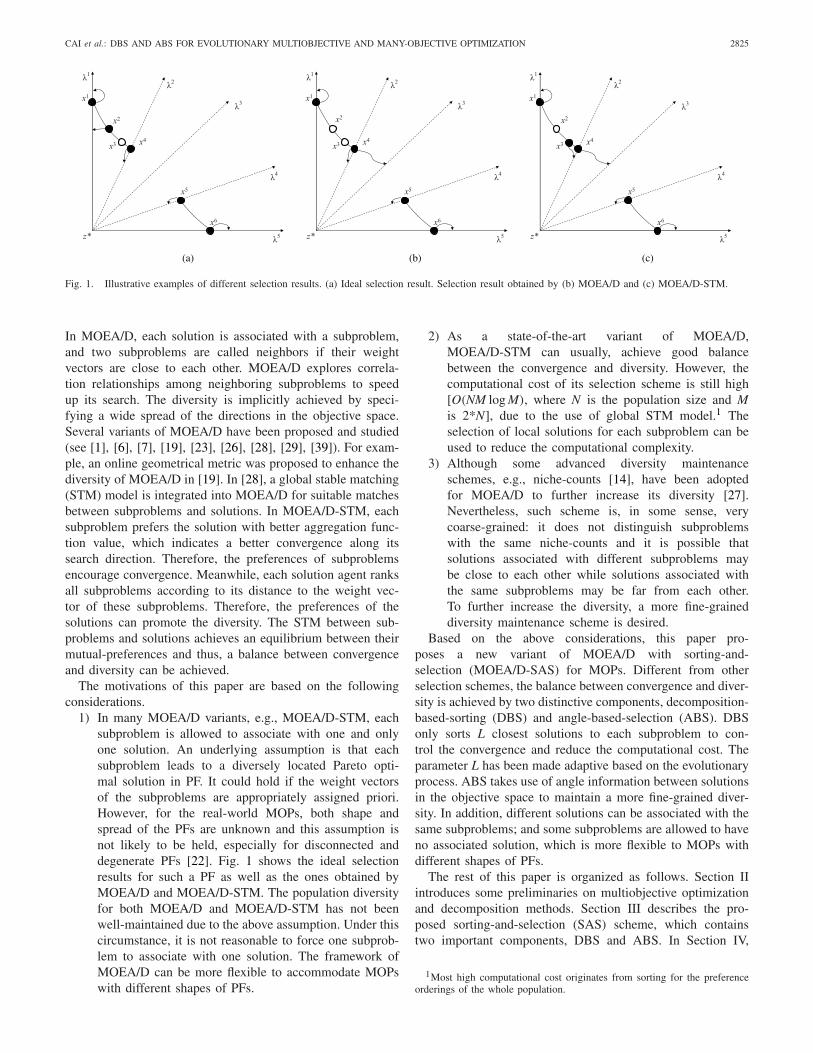
Fig. 1. Illustrative examples of different selection results. (a) Ideal selection result. Selection result obtained by (b) MOEA/D and (c) MOEA/D-STM.

In MOEA/D, each solution is associated with a subproblem,and two subproblems are called neighbors if their weightvectors are close to each other. MOEA/D explores correla-tion relationships among neighboring subproblems to speedup its search. The diversity is implicitly achieved by speci-fying a wide spread of the directions in the objective space.Several variants of MOEA/D have been proposed and studied(see [1], [6], [7], [19], [23], [26], [28], [29], [39]). For exam-ple, an online geometrical metric was proposed to enhance thediversity of MOEA/D in [19]. In [28], a global stable matching(STM) model is integrated into MOEA/D for suitable matchesbetween subproblems and solutions. In MOEA/D-STM, eachsubproblem prefers the solution with better aggregation func-tion value, which indicates a better convergence along itssearch direction. Therefore, the preferences of subproblemsencourage convergence. Meanwhile, each solution agent ranksall subproblems according to its distance to the weight vec-tor of these subproblems. Therefore, the preferences of thesolutions can promote the diversity. The STM between sub-problems and solutions achieves an equilibrium between theirmutual-preferences and thus, a balance between convergenceand diversity can be achieved.

The motivations of this paper are based on the followingconsiderations.

1) In many MOEA/D variants, e.g., MOEA/D-STM, eachsubproblem is allowed to associate with one and onlyone solution. An underlying assumption is that eachsubproblem leads to a diversely located Pareto opti-mal solution in PF. It could hold if the weight vectorsof the subproblems are appropriately assigned priori.However, for the real-world MOPs, both shape andspread of the PFs are unknown and this assumption isnot likely to be held, especially for disconnected anddegenerate PFs [22]. Fig. 1 shows the ideal selectionresults for such a PF as well as the ones obtained byMOEA/D and MOEA/D-STM. The population diversityfor both MOEA/D and MOEA/D-STM has not beenwell-maintained due to the above assumption. Under thiscircumstance, it is not reasonable to force one subprob-lem to associate with one solution. The framework ofMOEA/D can be more flexible to accommodate MOPswith different shapes of PFs.

2) As a state-of-the-art variant of MOEA/D,MOEA/D-STM can usually, achieve good balancebetween the convergence and diversity. However, thecomputational cost of its selection scheme is still high[O(NM log M), where N is the population size and Mis 2*N], due to the use of global STM model.1 Theselection of local solutions for each subproblem can beused to reduce the computational complexity.

3) Although some advanced diversity maintenanceschemes, e.g., niche-counts [14], have been adoptedfor MOEA/D to further increase its diversity [27].Nevertheless, such scheme is, in some sense, verycoarse-grained: it does not distinguish subproblemswith the same niche-counts and it is possible thatsolutions associated with different subproblems maybe close to each other while solutions associated withthe same subproblems may be far from each other.To further increase the diversity, a more fine-graineddiversity maintenance scheme is desired.

Based on the above considerations, this paper pro-poses a new variant of MOEA/D with sorting-and-selection (MOEA/D-SAS) for MOPs. Different from otherselection schemes, the balance between convergence and diver-sity is achieved by two distinctive components, decomposition-based-sorting (DBS) and angle-based-selection (ABS). DBSonly sorts L closest solutions to each subproblem to con-trol the convergence and reduce the computational cost. Theparameter L has been made adaptive based on the evolutionaryprocess. ABS takes use of angle information between solutionsin the objective space to maintain a more fine-grained diver-sity. In addition, different solutions can be associated with thesame subproblems; and some subproblems are allowed to haveno associated solution, which is more flexible to MOPs withdifferent shapes of PFs.

The rest of this paper is organized as follows. Section IIintroduces some preliminaries on multiobjective optimizationand decomposition methods. Section III describes the pro-posed sorting-and-selection (SAS) scheme, which containstwo important components, DBS and ABS. In Section IV,

1Most high computational cost originates from sorting for the preferenceorderings of the whole population.


SAS is integrated into MOEA/D. Section V introducesthe benchmark test functions and the performance indica-tors used in this paper. Experimental studies and discussionare presented in Section VI, where we compare our pro-posed algorithm with four classical MOEAs: 1) NSGA-II;2) MOSOPS-II; 3) MOEA/D; and 4) MOEA/D-DE; and threestate-of-the-art MOEA: 1) MOEA/D-STM; 2) NSGA-III; and3) MOEA/D-AWA on MOPs or many-objective optimizationproblem (MaOPs). The effects of DBS and ABS are also inves-tigated and discussed in Section VI. Section VII concludes thispaper.

II. PRELIMINARIES

This section first gives some basic definitions of multiob-jective optimization. Then, some basic knowledge about thedecomposition methods used in this paper is also introduced.

A. Basic Definitions

An MOP can be defined as follows:

minimize F(x) = (f1(x), . . . , fm(x))T

subject to x ∈ � (1)

where � is the decision space, F : � → Rm consists of mreal-valued objective functions. The attainable objective set is{F(x)|x ∈ �}.

Let u, v ∈ Rm, u is said to dominate v, denoted by u ≺ v,if and only if ui ≤ vi for every i ∈ {1, . . . , m} and uj < vj

for at least one index j ∈ {1, . . . , m}.2 A solution x∗ ∈ � isPareto-optimal to (1) if there exists no solution x ∈ � such thatF(x) dominates F(x∗). F(x∗) is then called a Pareto-optimal(objective) vector. In other words, any improvement in oneobjective of a Pareto-optimal solution is bound to deteriorateat least another objective.

B. Decomposition Methods

In principle, many methods can be used to decompose anMOP into a number of scalar optimization subproblems [30].Among them, the most popular ones are weighted sum (WS),Tchebycheff (TCH), and penalty boundary intersection (PBI)approaches [40]. The mathematical definition of these decom-position methods are as follows.

1) WS Approach: This approach considers a convex com-bination of all the objectives. One single objectivesubproblem sk is defined as

minimize gws(

x|λk)=

m∑i=1

λki fi(x)


where λk = (λk1, . . . , λ

km)T is the direction vector of sub-

problem sk, and λki ≥ 0, i ∈ 1, . . . , m and

∑mi=1 λk

i = 1.The optimal solution to (2) is a Pareto-optimal solutionto (1). A set of different Pareto-optimal solutions can beobtained simply by using different direction vectors, toapproximate the PF when it is convex.

2In the case of maximization, the inequality signs should be reversed.

2) TCH Approach: In this approach, one single objectivesubproblem sk is defined as

minimize gte(

x|λk, z∗)= max

1≤i≤m

{|fi(x)− z∗i |/λk

i

}


z∗ = (z∗1, . . . , z∗m)T is the ideal objective vector, wherez∗i < min{fi(x)|x ∈ �}, i ∈ 1, . . . , m. For convenience,λk

i = 0 is replaced by λki = 10−6, because λk

i = 0 is notallowed as a denominator in (3).

3) PBI Approach: This approach is a variant of normal-boundary intersection approach [11]. A subproblem sk

is defined as

minimize gpbi(

x|λk, z∗)= d1 + βd2

d1 =(F(x)− z∗

)Tλk/||λk||

d2 = ||F(x)− z∗ −(

d1/||λk||)λk||


where ||.|| denotes the L2-norm, and β is the penaltyparameter.

III. SELECTION OPERATORS

This section elaborates the selection operator based on theDBS and the ABS (SAS) scheme.

Given a set of N subproblems S and a set of M solutions,Z, the goal of SAS is to select N solutions from Z to form P.

For each subproblem j that has a direction vector λj, Pj(L)

denotes the set of the first L closest solutions to λj in Z. The“closeness” is defined by the acute angle between the solutionx and the direction vector λj, based on

angle(x, λj) = arccos

((F(x)− z∗)Tλj

‖F(x)− z∗‖‖λj‖

). (5)

The input parameter L in the current call of SAS has beenadaptive, based on the value of output α in the previous call ofSAS (see step 3 of Algorithm 4). L is defined as the numberof closest solutions to each subproblem and α is the numberof selected solution sets, which is explained in Section III-A.

A. Framework of SAS

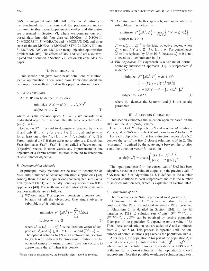
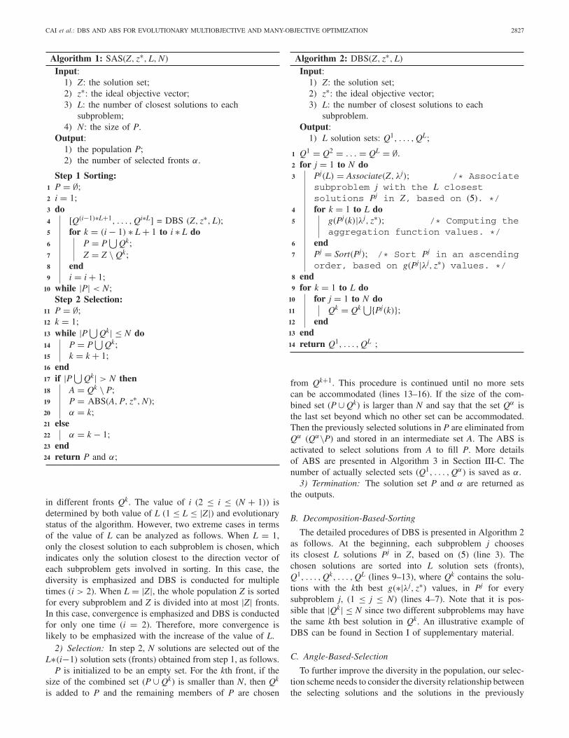
The pseudo-code of SAS is presented in Algorithm 1.1) Sorting: In step 1, P is first initialized to be an

empty set. The DBS is conducted iteratively. DBS, presentedin Algorithm 2, is detailed in Section III-B. In the ithiteration of DBS, L solution sets (fronts) Q(i−1)∗L+1, . . . ,

Q(i−1)∗L+j, . . . , Qi∗L can be obtained by sorting populationZ (or part of the population Z, depending on the value of L).Then, these sorted solution sets are added to P and eliminatedfrom Z (lines 5–8). This process is repeated until the totalnumber of sorted solutions |P| exceeds the population size N.

After step 1, the population Z (or part of the population Z) isdivided into L∗ (i−1) solution sets (fronts): Q1, . . . , QL∗(i−1),where i − 1 is the total number of iterations of DBS and Lis the number of closest solutions in the population Z to eachsubproblem. Note that possible overlapped solutions may exist


Algorithm 1: SAS(Z, z∗, L, N)Input:

1) Z: the solution set;2) z∗: the ideal objective vector;3) L: the number of closest solutions to each

subproblem;4) N: the size of P.

Output:1) the population P;2) the number of selected fronts α.

Step 1 Sorting:1 P = ∅;2 i = 1;3 do4 [Q(i−1)∗L+1, . . . , Qi∗L] = DBS (Z, z∗, L);5 for k = (i− 1) ∗ L+ 1 to i ∗ L do6 P = P

⋃Qk;

7 Z = Z \ Qk;8 end9 i = i+ 1;

10 while |P| < N;Step 2 Selection:

11 P = ∅;12 k = 1;13 while |P ⋃

Qk| ≤ N do14 P = P

⋃Qk;

15 k = k + 1;16 end17 if |P ⋃

Qk| > N then18 A = Qk \ P;19 P = ABS(A, P, z∗, N);20 α = k;21 else22 α = k − 1;23 end24 return P and α;

in different fronts Qk. The value of i (2 ≤ i ≤ (N + 1)) isdetermined by both value of L (1 ≤ L ≤ |Z|) and evolutionarystatus of the algorithm. However, two extreme cases in termsof the value of L can be analyzed as follows. When L = 1,only the closest solution to each subproblem is chosen, whichindicates only the solution closest to the direction vector ofeach subproblem gets involved in sorting. In this case, thediversity is emphasized and DBS is conducted for multipletimes (i > 2). When L = |Z|, the whole population Z is sortedfor every subproblem and Z is divided into at most |Z| fronts.In this case, convergence is emphasized and DBS is conductedfor only one time (i = 2). Therefore, more convergence islikely to be emphasized with the increase of the value of L.

2) Selection: In step 2, N solutions are selected out of theL∗(i−1) solution sets (fronts) obtained from step 1, as follows.

P is initialized to be an empty set. For the kth front, if thesize of the combined set (P ∪ Qk) is smaller than N, then Qk

is added to P and the remaining members of P are chosen

Algorithm 2: DBS(Z, z∗, L)Input:

1) Z: the solution set;2) z∗: the ideal objective vector;3) L: the number of closest solutions to each

subproblem.Output:

1) L solution sets: Q1, . . . , QL;

1 Q1 = Q2 = . . . = QL = ∅.2 for j = 1 to N do3 Pj(L) = Associate(Z, λj); /* Associate

subproblem j with the L closestsolutions Pj in Z, based on (5). */

4 for k = 1 to L do5 g(Pj(k)|λj, z∗); /* Computing the

aggregation function values. */6 end7 Pj = Sort(Pj); /* Sort Pj in an ascending

order, based on g(Pj|λj, z∗) values. */8 end9 for k = 1 to L do

10 for j = 1 to N do11 Qk = Qk ⋃{Pj(k)};12 end13 end14 return Q1, . . . , QL ;

from Qk+1. This procedure is continued until no more setscan be accommodated (lines 13–16). If the size of the com-bined set (P ∪Qk) is larger than N and say that the set Qα isthe last set beyond which no other set can be accommodated.Then the previously selected solutions in P are eliminated fromQα (Qα\P) and stored in an intermediate set A. The ABS isactivated to select solutions from A to fill P. More detailsof ABS are presented in Algorithm 3 in Section III-C. Thenumber of actually selected sets (Q1, . . . , Qα) is saved as α.

3) Termination: The solution set P and α are returned asthe outputs.

B. Decomposition-Based-Sorting

The detailed procedures of DBS is presented in Algorithm 2as follows. At the beginning, each subproblem j choosesits closest L solutions Pj in Z, based on (5) (line 3). Thechosen solutions are sorted into L solution sets (fronts),Q1, . . . , Qk, . . . , QL (lines 9–13), where Qk contains the solu-tions with the kth best g(∗|λj, z∗) values, in Pj for everysubproblem j, (1 ≤ j ≤ N) (lines 4–7). Note that it is pos-sible that |Qk| ≤ N since two different subproblems may havethe same kth best solution in Qk. An illustrative example ofDBS can be found in Section I of supplementary material.

C. Angle-Based-Selection

To further improve the diversity in the population, our selec-tion scheme needs to consider the diversity relationship betweenthe selecting solutions and the solutions in the previously


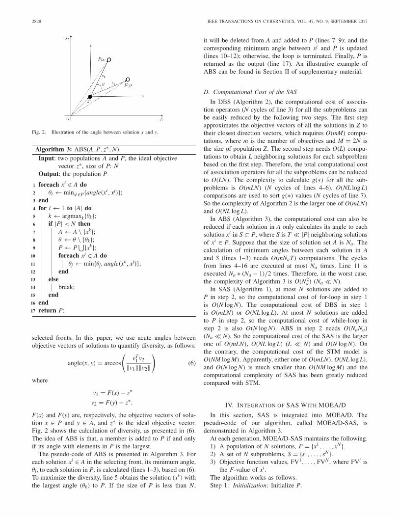
Fig. 2. Illustration of the angle between solution x and y.

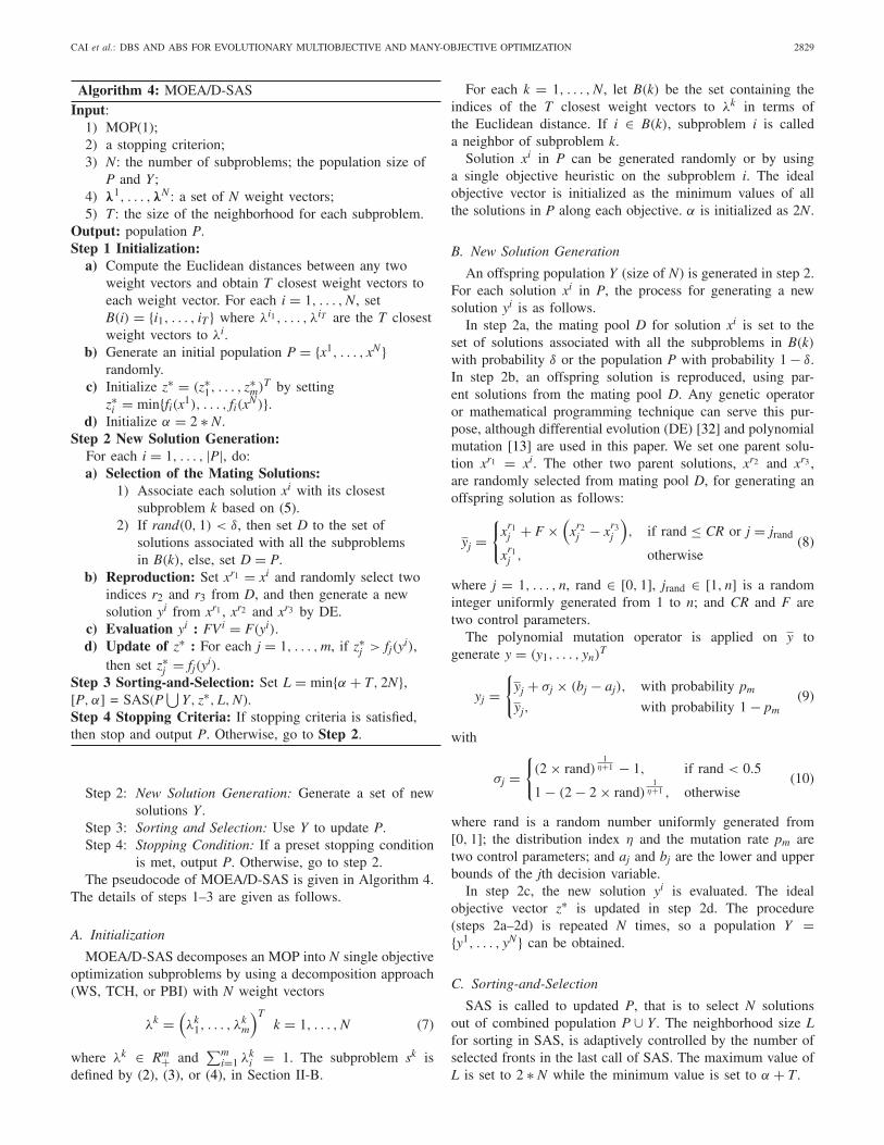
Algorithm 3: ABS(A, P, z∗, N)Input: two populations A and P, the ideal objective

vector z∗, size of P: NOutput: the population P

1 foreach xi ∈ A do2 θi ← minxj∈P{angle(xi, xj)};3 end4 for i← 1 to |A| do5 k← argmaxk{θk};6 if |P| < N then7 A← A \ {xk};8 θ ← θ \ {θk};9 P← P

⋃{xk};10 foreach xj ∈ A do11 θj ← min{θj, angle(xk, xj)};12 end13 else14 break;15 end16 end17 return P;

selected fronts. In this paper, we use acute angles betweenobjective vectors of solutions to quantify diversity, as follows:

angle(x, y) = arccos

(vT

1 v2

‖v1‖‖v2‖

)(6)

where

v1 = F(x)− z∗

v2 = F(y)− z∗.

F(x) and F(y) are, respectively, the objective vectors of solu-tion x ∈ P and y ∈ A, and z∗ is the ideal objective vector.Fig. 2 shows the calculation of diversity, as presented in (6).The idea of ABS is that, a member is added to P if and onlyif its angle with elements in P is the largest.

The pseudo-code of ABS is presented in Algorithm 3. Foreach solution xi ∈ A in the selecting front, its minimum angle,θi, to each solution in P, is calculated (lines 1–3), based on (6).To maximize the diversity, line 5 obtains the solution (xk) withthe largest angle (θk) to P. If the size of P is less than N,

it will be deleted from A and added to P (lines 7–9); and thecorresponding minimum angle between xj and P is updated(lines 10–12); otherwise, the loop is terminated. Finally, P isreturned as the output (line 17). An illustrative example ofABS can be found in Section II of supplementary material.

D. Computational Cost of the SAS

In DBS (Algorithm 2), the computational cost of associa-tion operators (N cycles of line 3) for all the subproblems canbe easily reduced by the following two steps. The first stepapproximates the objective vectors of all the solutions in Z totheir closest direction vectors, which requires O(mM) compu-tations, where m is the number of objectives and M = 2N isthe size of population Z. The second step needs O(L) compu-tations to obtain L neighboring solutions for each subproblembased on the first step. Therefore, the total computational costof association operators for all the subproblems can be reducedto O(LN). The complexity to calculate g(∗) for all the sub-problems is O(mLN) (N cycles of lines 4–6). O(NL log L)

comparisons are used to sort g(∗) values (N cycles of line 7).So the complexity of Algorithm 2 is the larger one of O(mLN)

and O(NL log L).In ABS (Algorithm 3), the computational cost can also be

reduced if each solution in A only calculates its angle to eachsolution xi in S ⊂ P, where S is T � |P| neighboring solutionsof xi ∈ P. Suppose that the size of solution set A is Na. Thecalculation of minimum angles between each solution in Aand S (lines 1–3) needs O(mNaT) computations. The cyclesfrom lines 4–16 are executed at most Na times. Line 11 isexecuted Na ∗ (Na − 1)/2 times. Therefore, in the worst case,the complexity of Algorithm 3 is O(N2

a) (Na � N).In SAS (Algorithm 1), at most N solutions are added to

P in step 2, so the computational cost of for-loop in step 1is O(N log N). The computational cost of DBS in step 1is O(mLN) or O(NL log L). At most N solutions are addedto P in step 2, so the computational cost of while-loop instep 2 is also O(N log N). ABS in step 2 needs O(NaNa)

(Na � N). So the computational cost of the SAS is the largerone of O(mLN), O(NL log L) (L � N) and O(N log N). Onthe contrary, the computational cost of the STM model isO(NM log M). Apparently, either one of O(mLN), O(NL log L),and O(N log N) is much smaller than O(NM log M) and thecomputational complexity of SAS has been greatly reducedcompared with STM.

IV. INTEGRATION OF SAS WITH MOEA/D

In this section, SAS is integrated into MOEA/D. Thepseudo-code of our algorithm, called MOEA/D-SAS, isdemonstrated in Algorithm 3.

At each generation, MOEA/D-SAS maintains the following.1) A population of N solutions, P = {x1, . . . , xN}.2) A set of N subproblems, S = {s1, . . . , sN}.3) Objective function values, FV1, . . . , FVN , where FVi is

the F-value of xi.The algorithm works as follows.Step 1: Initialization: Initialize P.


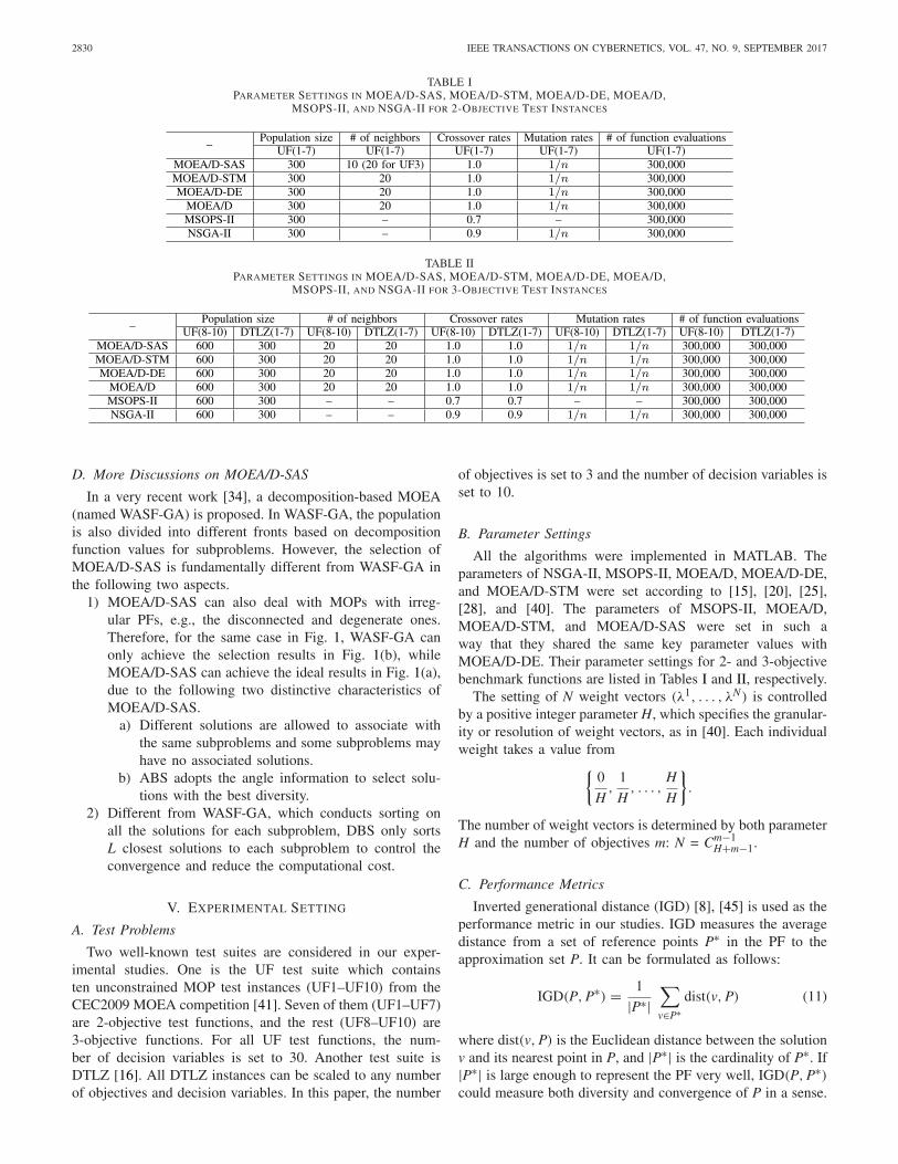
Algorithm 4: MOEA/D-SASInput:

1) MOP(1);2) a stopping criterion;3) N: the number of subproblems; the population size of

P and Y;4) λ1, . . . ,λN : a set of N weight vectors;5) T: the size of the neighborhood for each subproblem.

Output: population P.Step 1 Initialization:

a) Compute the Euclidean distances between any twoweight vectors and obtain T closest weight vectors toeach weight vector. For each i = 1, . . . , N, setB(i) = {i1, . . . , iT} where λi1, . . . , λiT are the T closestweight vectors to λi.

b) Generate an initial population P = {x1, . . . , xN}randomly.

c) Initialize z∗ = (z∗1, . . . , z∗m)T by settingz∗i = min{fi(x1), . . . , fi(xN)}.

d) Initialize α = 2 ∗ N.Step 2 New Solution Generation:

For each i = 1, . . . , |P|, do:a) Selection of the Mating Solutions:

1) Associate each solution xi with its closestsubproblem k based on (5).

2) If rand(0, 1) < δ, then set D to the set ofsolutions associated with all the subproblemsin B(k), else, set D = P.

b) Reproduction: Set xr1 = xi and randomly select twoindices r2 and r3 from D, and then generate a newsolution yi from xr1 , xr2 and xr3 by DE.

c) Evaluation yi : FVi = F(yi).d) Update of z∗ : For each j = 1, . . . , m, if z∗j > fj(yi),

then set z∗j = fj(yi).Step 3 Sorting-and-Selection: Set L = min{α + T, 2N},[P, α] = SAS(P

⋃Y, z∗, L, N).

Step 4 Stopping Criteria: If stopping criteria is satisfied,then stop and output P. Otherwise, go to Step 2.

Step 2: New Solution Generation: Generate a set of newsolutions Y .

Step 3: Sorting and Selection: Use Y to update P.Step 4: Stopping Condition: If a preset stopping condition

is met, output P. Otherwise, go to step 2.The pseudocode of MOEA/D-SAS is given in Algorithm 4.

The details of steps 1–3 are given as follows.

A. Initialization

MOEA/D-SAS decomposes an MOP into N single objectiveoptimization subproblems by using a decomposition approach(WS, TCH, or PBI) with N weight vectors

λk =(λk

1, . . . , λkm

)Tk = 1, . . . , N (7)

where λk ∈ Rm+ and∑m

i=1 λki = 1. The subproblem sk is

defined by (2), (3), or (4), in Section II-B.

For each k = 1, . . . , N, let B(k) be the set containing theindices of the T closest weight vectors to λk in terms ofthe Euclidean distance. If i ∈ B(k), subproblem i is calleda neighbor of subproblem k.

Solution xi in P can be generated randomly or by usinga single objective heuristic on the subproblem i. The idealobjective vector is initialized as the minimum values of allthe solutions in P along each objective. α is initialized as 2N.

B. New Solution Generation

An offspring population Y (size of N) is generated in step 2.For each solution xi in P, the process for generating a newsolution yi is as follows.

In step 2a, the mating pool D for solution xi is set to theset of solutions associated with all the subproblems in B(k)with probability δ or the population P with probability 1− δ.In step 2b, an offspring solution is reproduced, using par-ent solutions from the mating pool D. Any genetic operatoror mathematical programming technique can serve this pur-pose, although differential evolution (DE) [32] and polynomialmutation [13] are used in this paper. We set one parent solu-tion xr1 = xi. The other two parent solutions, xr2 and xr3 ,are randomly selected from mating pool D, for generating anoffspring solution as follows:

yj ={

xr1j + F ×

(xr2

j − xr3j

), if rand ≤ CR or j = jrand

xr1j , otherwise

(8)

where j = 1, . . . , n, rand ∈ [0, 1], jrand ∈ [1, n] is a randominteger uniformly generated from 1 to n; and CR and F aretwo control parameters.

The polynomial mutation operator is applied on y togenerate y = (y1, . . . , yn)

T

yj ={

yj + σj × (bj − aj), with probability pm

yj, with probability 1− pm(9)

with

σj ={

(2× rand)1

η+1 − 1, if rand < 0.5

1− (2− 2× rand)1

η+1 , otherwise(10)

where rand is a random number uniformly generated from[0, 1]; the distribution index η and the mutation rate pm aretwo control parameters; and aj and bj are the lower and upperbounds of the jth decision variable.

In step 2c, the new solution yi is evaluated. The idealobjective vector z∗ is updated in step 2d. The procedure(steps 2a–2d) is repeated N times, so a population Y ={y1, . . . , yN} can be obtained.

C. Sorting-and-Selection

SAS is called to updated P, that is to select N solutionsout of combined population P ∪ Y . The neighborhood size Lfor sorting in SAS, is adaptively controlled by the number ofselected fronts in the last call of SAS. The maximum value ofL is set to 2 ∗ N while the minimum value is set to α + T .


TABLE IPARAMETER SETTINGS IN MOEA/D-SAS, MOEA/D-STM, MOEA/D-DE, MOEA/D,

MSOPS-II, AND NSGA-II FOR 2-OBJECTIVE TEST INSTANCES

TABLE IIPARAMETER SETTINGS IN MOEA/D-SAS, MOEA/D-STM, MOEA/D-DE, MOEA/D,

MSOPS-II, AND NSGA-II FOR 3-OBJECTIVE TEST INSTANCES

D. More Discussions on MOEA/D-SAS

In a very recent work [34], a decomposition-based MOEA(named WASF-GA) is proposed. In WASF-GA, the populationis also divided into different fronts based on decompositionfunction values for subproblems. However, the selection ofMOEA/D-SAS is fundamentally different from WASF-GA inthe following two aspects.

1) MOEA/D-SAS can also deal with MOPs with irreg-ular PFs, e.g., the disconnected and degenerate ones.Therefore, for the same case in Fig. 1, WASF-GA canonly achieve the selection results in Fig. 1(b), whileMOEA/D-SAS can achieve the ideal results in Fig. 1(a),due to the following two distinctive characteristics ofMOEA/D-SAS.

a) Different solutions are allowed to associate withthe same subproblems and some subproblems mayhave no associated solutions.

b) ABS adopts the angle information to select solu-tions with the best diversity.

2) Different from WASF-GA, which conducts sorting onall the solutions for each subproblem, DBS only sortsL closest solutions to each subproblem to control theconvergence and reduce the computational cost.

V. EXPERIMENTAL SETTING

A. Test Problems

Two well-known test suites are considered in our exper-imental studies. One is the UF test suite which containsten unconstrained MOP test instances (UF1–UF10) from theCEC2009 MOEA competition [41]. Seven of them (UF1–UF7)are 2-objective test functions, and the rest (UF8–UF10) are3-objective functions. For all UF test functions, the num-ber of decision variables is set to 30. Another test suite isDTLZ [16]. All DTLZ instances can be scaled to any numberof objectives and decision variables. In this paper, the number

of objectives is set to 3 and the number of decision variables isset to 10.

B. Parameter Settings

All the algorithms were implemented in MATLAB. Theparameters of NSGA-II, MSOPS-II, MOEA/D, MOEA/D-DE,and MOEA/D-STM were set according to [15], [20], [25],[28], and [40]. The parameters of MSOPS-II, MOEA/D,MOEA/D-STM, and MOEA/D-SAS were set in such away that they shared the same key parameter values withMOEA/D-DE. Their parameter settings for 2- and 3-objectivebenchmark functions are listed in Tables I and II, respectively.

The setting of N weight vectors (λ1, . . . , λN) is controlledby a positive integer parameter H, which specifies the granular-ity or resolution of weight vectors, as in [40]. Each individualweight takes a value from

{0

H,

1

H, . . . ,

H

H

}.

The number of weight vectors is determined by both parameterH and the number of objectives m: N = Cm−1

H+m−1.

C. Performance Metrics

Inverted generational distance (IGD) [8], [45] is used as theperformance metric in our studies. IGD measures the averagedistance from a set of reference points P∗ in the PF to theapproximation set P. It can be formulated as follows:

IGD(P, P∗) = 1

|P∗|∑v∈P∗

dist(v, P) (11)

where dist(v, P) is the Euclidean distance between the solutionv and its nearest point in P, and |P∗| is the cardinality of P∗. If|P∗| is large enough to represent the PF very well, IGD(P, P∗)could measure both diversity and convergence of P in a sense.


TABLE IIIMEAN AND STANDARD DEVIATION VALUES OF IGD, OBTAINED BY MOEA/D-SAS, MOEA/D,

MOEA/D-DE, MSOPS-II, AND NSGA-II ON UF AND DTLZ INSTANCES

VI. EXPERIMENTAL STUDIES AND DISCUSSION

To study the performance of MOEA/D-SAS and understandits behavior, this section conducts the following experimentalworks.

1) Comparisons of MOEA/D-SAS with NSGA-II [15],MOEA/D [40], MOEA/D-DE [25], and MSOPS-II [20].

2) Comparisons of MOEA/D-SAS with MOEA/D-STM [28].

3) Investigation of the computational efficiency of DBS.4) Investigation of the effects of ABS in MOEA/D-SAS.In our experiments, each algorithm was run 30 times inde-

pendently for each test instance. To make fair comparisons,TCH approach has been used as decomposition approachin MOEA/D, MOEA/D-DE, and MOEA/D-SAS on 2- or3-objective optimization problems.

A. Comparisons With Classical MOEAs

In this section, we compare MOEA/D-SAS with four clas-sical domination or decomposition-based MOEAs—NSGA-II,MSOPS-II, MOEA/D, and MOEA/D-DE.

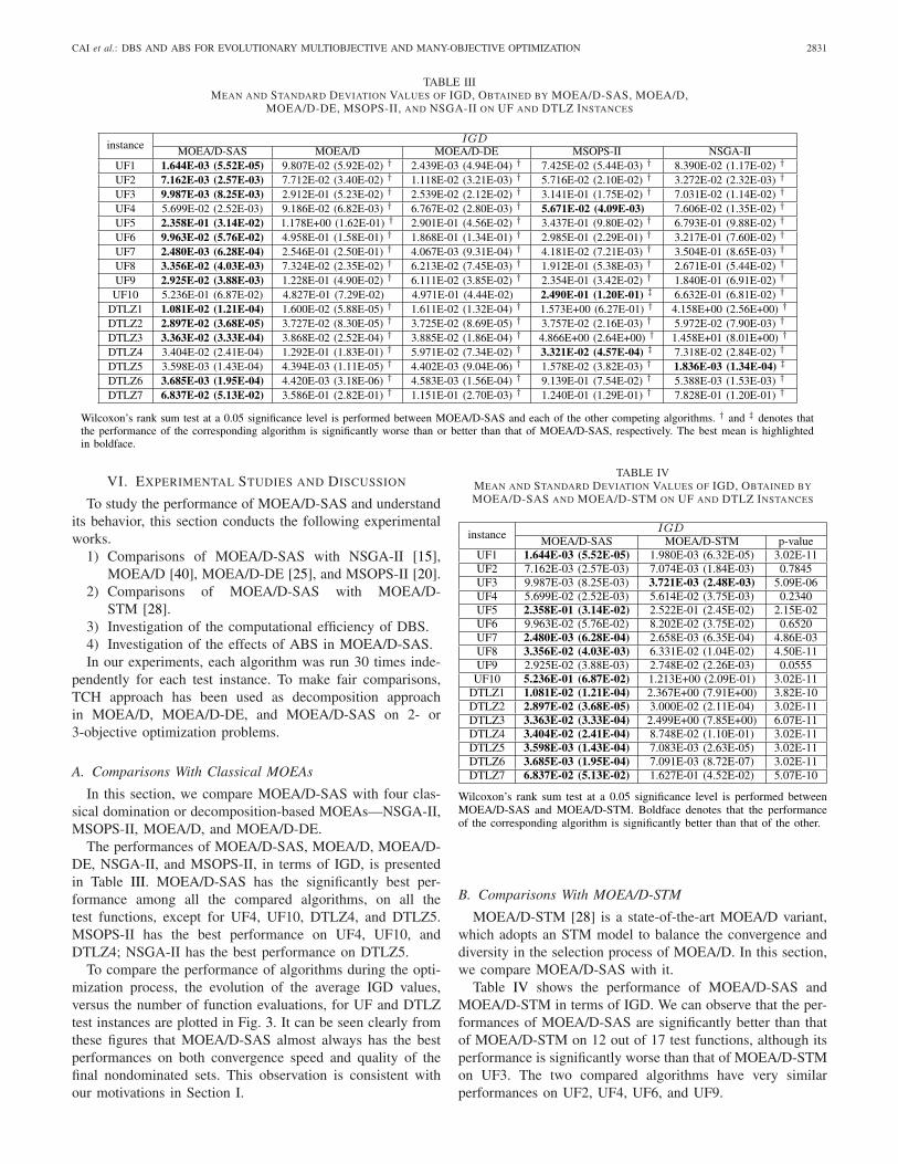
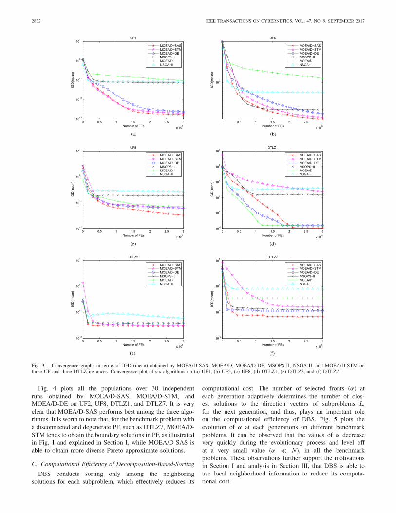
The performances of MOEA/D-SAS, MOEA/D, MOEA/D-DE, NSGA-II, and MSOPS-II, in terms of IGD, is presentedin Table III. MOEA/D-SAS has the significantly best per-formance among all the compared algorithms, on all thetest functions, except for UF4, UF10, DTLZ4, and DTLZ5.MSOPS-II has the best performance on UF4, UF10, andDTLZ4; NSGA-II has the best performance on DTLZ5.

To compare the performance of algorithms during the opti-mization process, the evolution of the average IGD values,versus the number of function evaluations, for UF and DTLZtest instances are plotted in Fig. 3. It can be seen clearly fromthese figures that MOEA/D-SAS almost always has the bestperformances on both convergence speed and quality of thefinal nondominated sets. This observation is consistent withour motivations in Section I.

TABLE IVMEAN AND STANDARD DEVIATION VALUES OF IGD, OBTAINED BY

MOEA/D-SAS AND MOEA/D-STM ON UF AND DTLZ INSTANCES

B. Comparisons With MOEA/D-STM

MOEA/D-STM [28] is a state-of-the-art MOEA/D variant,which adopts an STM model to balance the convergence anddiversity in the selection process of MOEA/D. In this section,we compare MOEA/D-SAS with it.

Table IV shows the performance of MOEA/D-SAS andMOEA/D-STM in terms of IGD. We can observe that the per-formances of MOEA/D-SAS are significantly better than thatof MOEA/D-STM on 12 out of 17 test functions, although itsperformance is significantly worse than that of MOEA/D-STMon UF3. The two compared algorithms have very similarperformances on UF2, UF4, UF6, and UF9.


Fig. 3. Convergence graphs in terms of IGD (mean) obtained by MOEA/D-SAS, MOEA/D, MOEA/D-DE, MSOPS-II, NSGA-II, and MOEA/D-STM onthree UF and three DTLZ instances. Convergence plot of six algorithms on (a) UF1, (b) UF5, (c) UF8, (d) DTLZ1, (e) DTLZ2, and (f) DTLZ7.

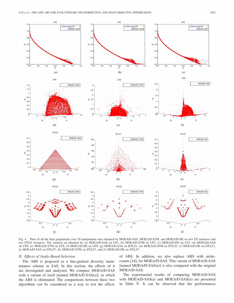
Fig. 4 plots all the populations over 30 independentruns obtained by MOEA/D-SAS, MOEA/D-STM, andMOEA/D-DE on UF2, UF8, DTLZ1, and DTLZ7. It is veryclear that MOEA/D-SAS performs best among the three algo-rithms. It is worth to note that, for the benchmark problem witha disconnected and degenerate PF, such as DTLZ7, MOEA/D-STM tends to obtain the boundary solutions in PF, as illustratedin Fig. 1 and explained in Section I, while MOEA/D-SAS isable to obtain more diverse Pareto approximate solutions.

C. Computational Efficiency of Decomposition-Based-Sorting

DBS conducts sorting only among the neighboringsolutions for each subproblem, which effectively reduces its

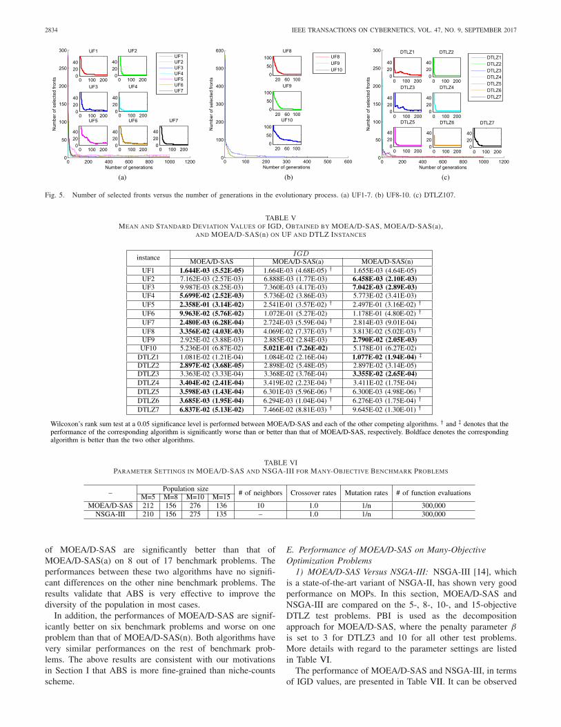
computational cost. The number of selected fronts (α) ateach generation adaptively determines the number of clos-est solutions to the direction vectors of subproblems L,for the next generation, and thus, plays an important roleon the computational efficiency of DBS. Fig. 5 plots theevolution of α at each generations on different benchmarkproblems. It can be observed that the values of α decreasevery quickly during the evolutionary process and level offat a very small value (α � N), in all the benchmarkproblems. These observations further support the motivationsin Section I and analysis in Section III, that DBS is able touse local neighborhood information to reduce its computa-tional cost.


Fig. 4. Plots of all the final populations over 30 independent runs obtained by MOEA/D-SAS, MOEA/D-STM, and MOEA/D-DE on two UF instances andtwo DTLZ instances. The solution set obtained by (a) MOEA/D-SAS on UF2, (b) MOEA/D-STM on UF2, (c) MOEA/D-DE on UF2, (d) MOEA/D-SASon UF8, (e) MOEA/D-STM on UF8, (f) MOEA/D-DE on UF8, (g) MOEA/D-SAS on DTLZ1, (h) MOEA/D-STM on DTLZ1, (i) MOEA/D-DE on DTLZ1,(j) MOEA/D-SAS on DTLZ7, (k) MOEA/D-STM on DTLZ7, and (l) MOEA/D-DE on DTLZ7.

D. Effects of Angle-Based-SelectionThe ABS is proposed as a fine-grained diversity main-

tenance scheme in SAS. In this section, the effects of itare investigated and analyzed. We compare MOEA/D-SASwith a variant of itself [named MOEA/D-SAS(a)], in whichthe ABS is eliminated. The comparisons between these twoalgorithms can be considered as a way to test the effects

of ABS. In addition, we also replace ABS with niche-counts [14], for MOEA/D-SAS. This variant of MOEA/D-SAS[named MOEA/D-SAS(n)] is also compared with the originalMOEA/D-SAS.

The experimental results of comparing MOEA/D-SASwith MOEA/D-SAS(a) and MOEA/D-SAS(n) are presentedin Table V. It can be observed that the performances


Fig. 5. Number of selected fronts versus the number of generations in the evolutionary process. (a) UF1-7. (b) UF8-10. (c) DTLZ107.

TABLE VMEAN AND STANDARD DEVIATION VALUES OF IGD, OBTAINED BY MOEA/D-SAS, MOEA/D-SAS(a),

AND MOEA/D-SAS(n) ON UF AND DTLZ INSTANCES

TABLE VIPARAMETER SETTINGS IN MOEA/D-SAS AND NSGA-III FOR MANY-OBJECTIVE BENCHMARK PROBLEMS

of MOEA/D-SAS are significantly better than that ofMOEA/D-SAS(a) on 8 out of 17 benchmark problems. Theperformances between these two algorithms have no signifi-cant differences on the other nine benchmark problems. Theresults validate that ABS is very effective to improve thediversity of the population in most cases.

In addition, the performances of MOEA/D-SAS are signif-icantly better on six benchmark problems and worse on oneproblem than that of MOEA/D-SAS(n). Both algorithms havevery similar performances on the rest of benchmark prob-lems. The above results are consistent with our motivationsin Section I that ABS is more fine-grained than niche-countsscheme.

E. Performance of MOEA/D-SAS on Many-ObjectiveOptimization Problems

1) MOEA/D-SAS Versus NSGA-III: NSGA-III [14], whichis a state-of-the-art variant of NSGA-II, has shown very goodperformance on MOPs. In this section, MOEA/D-SAS andNSGA-III are compared on the 5-, 8-, 10-, and 15-objectiveDTLZ test problems. PBI is used as the decompositionapproach for MOEA/D-SAS, where the penalty parameter β

is set to 3 for DTLZ3 and 10 for all other test problems.More details with regard to the parameter settings are listedin Table VI.

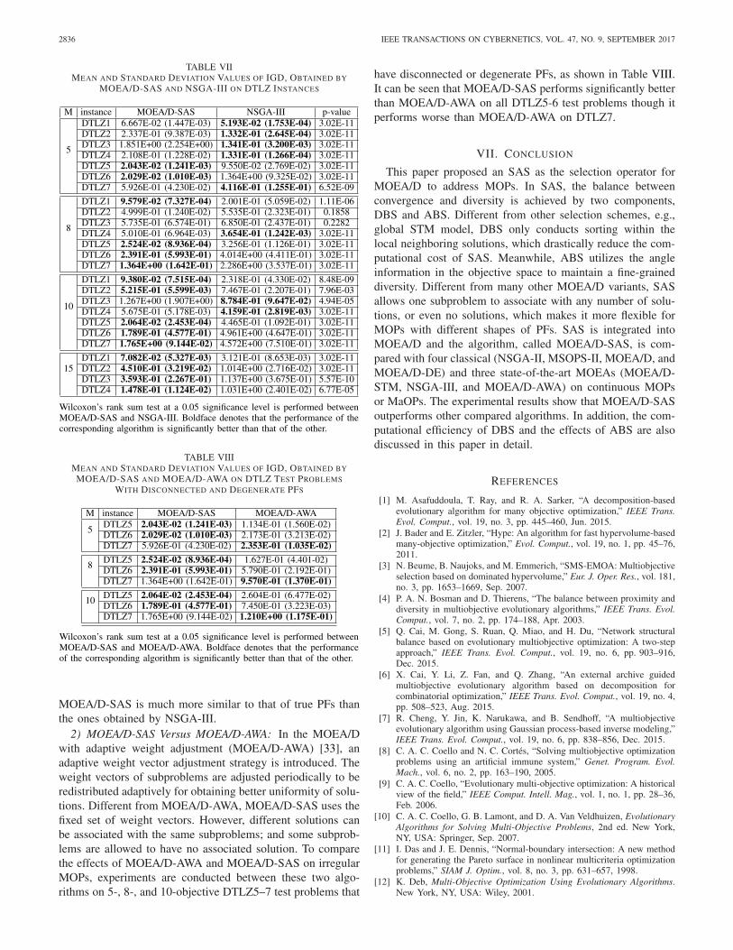
The performance of MOEA/D-SAS and NSGA-III, in termsof IGD values, are presented in Table VII. It can be observed


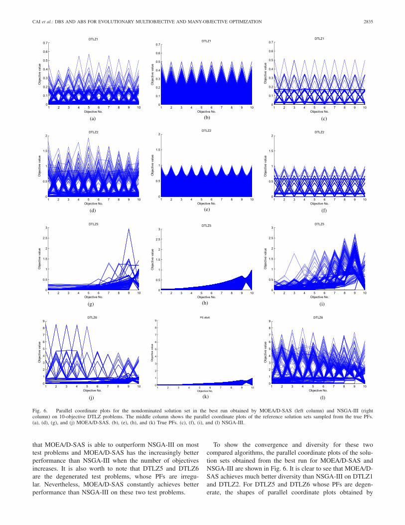
Fig. 6. Parallel coordinate plots for the nondominated solution set in the best run obtained by MOEA/D-SAS (left column) and NSGA-III (rightcolumn) on 10-objective DTLZ problems. The middle column shows the parallel coordinate plots of the reference solution sets sampled from the true PFs.(a), (d), (g), and (j) MOEA/D-SAS. (b), (e), (h), and (k) True PFs. (c), (f), (i), and (l) NSGA-III.

that MOEA/D-SAS is able to outperform NSGA-III on mosttest problems and MOEA/D-SAS has the increasingly betterperformance than NSGA-III when the number of objectivesincreases. It is also worth to note that DTLZ5 and DTLZ6are the degenerated test problems, whose PFs are irregu-lar. Nevertheless, MOEA/D-SAS constantly achieves betterperformance than NSGA-III on these two test problems.

To show the convergence and diversity for these twocompared algorithms, the parallel coordinate plots of the solu-tion sets obtained from the best run for MOEA/D-SAS andNSGA-III are shown in Fig. 6. It is clear to see that MOEA/D-SAS achieves much better diversity than NSGA-III on DTLZ1and DTLZ2. For DTLZ5 and DTLZ6 whose PFs are degen-erate, the shapes of parallel coordinate plots obtained by


TABLE VIIMEAN AND STANDARD DEVIATION VALUES OF IGD, OBTAINED BY

MOEA/D-SAS AND NSGA-III ON DTLZ INSTANCES

TABLE VIIIMEAN AND STANDARD DEVIATION VALUES OF IGD, OBTAINED BY

MOEA/D-SAS AND MOEA/D-AWA ON DTLZ TEST PROBLEMS

WITH DISCONNECTED AND DEGENERATE PFS

MOEA/D-SAS is much more similar to that of true PFs thanthe ones obtained by NSGA-III.

2) MOEA/D-SAS Versus MOEA/D-AWA: In the MOEA/Dwith adaptive weight adjustment (MOEA/D-AWA) [33], anadaptive weight vector adjustment strategy is introduced. Theweight vectors of subproblems are adjusted periodically to beredistributed adaptively for obtaining better uniformity of solu-tions. Different from MOEA/D-AWA, MOEA/D-SAS uses thefixed set of weight vectors. However, different solutions canbe associated with the same subproblems; and some subprob-lems are allowed to have no associated solution. To comparethe effects of MOEA/D-AWA and MOEA/D-SAS on irregularMOPs, experiments are conducted between these two algo-rithms on 5-, 8-, and 10-objective DTLZ5–7 test problems that

have disconnected or degenerate PFs, as shown in Table VIII.It can be seen that MOEA/D-SAS performs significantly betterthan MOEA/D-AWA on all DTLZ5-6 test problems though itperforms worse than MOEA/D-AWA on DTLZ7.

VII. CONCLUSION

This paper proposed an SAS as the selection operator forMOEA/D to address MOPs. In SAS, the balance betweenconvergence and diversity is achieved by two components,DBS and ABS. Different from other selection schemes, e.g.,global STM model, DBS only conducts sorting within thelocal neighboring solutions, which drastically reduce the com-putational cost of SAS. Meanwhile, ABS utilizes the angleinformation in the objective space to maintain a fine-graineddiversity. Different from many other MOEA/D variants, SASallows one subproblem to associate with any number of solu-tions, or even no solutions, which makes it more flexible forMOPs with different shapes of PFs. SAS is integrated intoMOEA/D and the algorithm, called MOEA/D-SAS, is com-pared with four classical (NSGA-II, MSOPS-II, MOEA/D, andMOEA/D-DE) and three state-of-the-art MOEAs (MOEA/D-STM, NSGA-III, and MOEA/D-AWA) on continuous MOPsor MaOPs. The experimental results show that MOEA/D-SASoutperforms other compared algorithms. In addition, the com-putational efficiency of DBS and the effects of ABS are alsodiscussed in this paper in detail.

REFERENCES

[1] M. Asafuddoula, T. Ray, and R. A. Sarker, “A decomposition-basedevolutionary algorithm for many objective optimization,” IEEE Trans.Evol. Comput., vol. 19, no. 3, pp. 445–460, Jun. 2015.

[2] J. Bader and E. Zitzler, “Hype: An algorithm for fast hypervolume-basedmany-objective optimization,” Evol. Comput., vol. 19, no. 1, pp. 45–76,2011.

[3] N. Beume, B. Naujoks, and M. Emmerich, “SMS-EMOA: Multiobjectiveselection based on dominated hypervolume,” Eur. J. Oper. Res., vol. 181,no. 3, pp. 1653–1669, Sep. 2007.

[4] P. A. N. Bosman and D. Thierens, “The balance between proximity anddiversity in multiobjective evolutionary algorithms,” IEEE Trans. Evol.Comput., vol. 7, no. 2, pp. 174–188, Apr. 2003.

[5] Q. Cai, M. Gong, S. Ruan, Q. Miao, and H. Du, “Network structuralbalance based on evolutionary multiobjective optimization: A two-stepapproach,” IEEE Trans. Evol. Comput., vol. 19, no. 6, pp. 903–916,Dec. 2015.

[6] X. Cai, Y. Li, Z. Fan, and Q. Zhang, “An external archive guidedmultiobjective evolutionary algorithm based on decomposition forcombinatorial optimization,” IEEE Trans. Evol. Comput., vol. 19, no. 4,pp. 508–523, Aug. 2015.

[7] R. Cheng, Y. Jin, K. Narukawa, and B. Sendhoff, “A multiobjectiveevolutionary algorithm using Gaussian process-based inverse modeling,”IEEE Trans. Evol. Comput., vol. 19, no. 6, pp. 838–856, Dec. 2015.

[8] C. A. C. Coello and N. C. Cortés, “Solving multiobjective optimizationproblems using an artificial immune system,” Genet. Program. Evol.Mach., vol. 6, no. 2, pp. 163–190, 2005.

[9] C. A. C. Coello, “Evolutionary multi-objective optimization: A historicalview of the field,” IEEE Comput. Intell. Mag., vol. 1, no. 1, pp. 28–36,Feb. 2006.

[10] C. A. C. Coello, G. B. Lamont, and D. A. Van Veldhuizen, EvolutionaryAlgorithms for Solving Multi-Objective Problems, 2nd ed. New York,NY, USA: Springer, Sep. 2007.

[11] I. Das and J. E. Dennis, “Normal-boundary intersection: A new methodfor generating the Pareto surface in nonlinear multicriteria optimizationproblems,” SIAM J. Optim., vol. 8, no. 3, pp. 631–657, 1998.

[12] K. Deb, Multi-Objective Optimization Using Evolutionary Algorithms.New York, NY, USA: Wiley, 2001.


[13] K. Deb and M. Goyal, “A combined genetic adaptive search (GeneAS)for engineering design,” Comput. Sci. Informat., vol. 26, no. 4,pp. 30–45, 1996.

[14] K. Deb and H. Jain, “An evolutionary many-objective optimizationalgorithm using reference-point-based nondominated sorting approach,part I: Solving problems with box constraints,” IEEE Trans. Evol.Comput., vol. 18, no. 4, pp. 577–601, Aug. 2014.

[15] K. Deb, A. Pratap, S. Agarwal, and T. Meyarivan, “A fast and elitistmultiobjective genetic algorithm: NSGA-II,” IEEE Trans. Evol. Comput.,vol. 6, no. 2, pp. 182–197, Apr. 2002.

[16] K. Deb, L. Thiele, M. Laumanns, and E. Zitzler, “Scalable test prob-lems for evolutionary multiobjective optimization,” EvolutionaryMultiobjective Optimization. London, U.K.: Springer, 2005,pp. 105–145.

[17] J. J. Durillo, A. J. Nebro, F. Luna, and E. Alba, “On the effect of thesteady-state selection scheme in multi-objective genetic algorithms,” inProc. 5th Int. Conf. Evol. Multi-Criterion Optim. (EMO), vol. 5467.Nantes, France, Apr. 2009, pp. 183–197.

[18] C. M. Fonseca and P. J. Fleming, “An overview of evolutionary algo-rithms in multiobjective optimization,” Evol. Comput., vol. 3, no. 1,pp. 1–16, 1995.

[19] S. B. Gee, K. C. Tan, V. A. Shim, and N. R. Pal, “Online diversityassessment in evolutionary multiobjective optimization: A geometricalperspective,” IEEE Trans. Evol. Comput., vol. 19, no. 4, pp. 542–559,Aug. 2015.

[20] E. J. Hughes, “MSOPS-II: A general-purpose many-objective optimiser,”in Proc. IEEE Congr. Evol. Comput. (CEC), Singapore, Sep. 2007,pp. 3944–3951.

[21] E. J. Hughes, “Multiple single objective Pareto sampling,” in Proc.Congr. Evol. Comput. (CEC), vol. 4. Canberra, ACT, Australia,Dec. 2003, pp. 2678–2684.

[22] H. Ishibuchi, H. Masuda, and Y. Nojima, “Pareto fronts of many-objective degenerate test problems,” IEEE Trans. Evol. Comput., to bepublished.

[23] H. Ishibuchi, Y. Sakane, N. Tsukamoto, and Y. Nojima, “Adaptationof scalarizing functions in MOEA/D: An adaptive scalarizing function-based multiobjective evolutionary algorithm,” in Proc. 5th Int. Conf.Evol. Multi Criterion Optim. (EMO), vol. 5467. Nantes, France,Apr. 2009, pp. 438–452.

[24] B. Li, K. Tang, J. Li, and X. Yao, “Stochastic ranking algorithm formany-objective optimization based on multiple indicators,” IEEE Trans.Evol. Comput., Mar. 2016, doi: 10.1109/TEVC.2016.2549267. .

[25] H. Li and Q. Zhang, “Multiobjective optimization problems with compli-cated Pareto sets, MOEA/D and NSGA-II,” IEEE Trans. Evol. Comput.,vol. 13, no. 2, pp. 284–302, Apr. 2009.

[26] K. Li, K. Deb, Q. Zhang, and S. Kwong, “An evolutionary many-objective optimization algorithm based on dominance and decompo-sition,” IEEE Trans. Evol. Comput., vol. 19, no. 5, pp. 694–716,Oct. 2015.

[27] K. Li, S. Kwong, Q. Zhang, and K. Deb, “Inter-relationship basedselection for decomposition multiobjective optimization,” IEEE Trans.Cybern., vol. 45, no. 10, pp. 2076–2088, Oct. 2015.

[28] K. Li, Q. Zhang, S. Kwong, M. Li, and R. Wang, “Stable matching-basedselection in evolutionary multiobjective optimization,” IEEE Trans. Evol.Comput., vol. 18, no. 6, pp. 909–923, Dec. 2014.

[29] H.-L. Liu, F. Gu, and Q. Zhang, “Decomposition of a multiobjectiveoptimization problem into a number of simple multiobjective sub-problems,” IEEE Trans. Evol. Comput., vol. 18, no. 3, pp. 450–455,Jun. 2014.

[30] K. Miettinen, Nonlinear Multiobjective Optimization. Boston, MA,USA: Kluwer Academic, 1999.

[31] T. Murata, H. Ishibuchi, and M. Gen, “Specification of genetic searchdirections in cellular multi-objective genetic algorithms,” in Proc. 1stInt. Conf. Evol. Multi-Criterion Optim., Zürich, Switzerland, 2001,pp. 82–95.

[32] K. Price, R. M. Storn, and J. A. Lampinen, Differential Evolution:A Practical Approach to Global Optimization (Natural ComputingSeries). Heidelberg, Germany: Springer, 2005.

[33] Y. Qi et al., “MOEA/D with adaptive weight adjustment,” Evol. Comput.,vol. 22, no. 2, pp. 231–264, 2014.

[34] A. B. Ruiz, R. Saborido, and M. Luque, “A preference-basedevolutionary algorithm for multiobjective optimization: The weightingachievement scalarizing function genetic algorithm,” J. Glob. Optim.,vol. 62, no. 1, pp. 101–129, 2015.

[35] J. D. Schaffer and J. J. Grefenstette, “Multi-objective learning viagenetic algorithms,” in Proc. 9th Int. Joint Conf. Artif. Intell. (IJCAI),Los Angeles, CA, USA, 1985, pp. 593–595.

[36] X.-N. Shen and X. Yao, “Mathematical modeling and multi-objectiveevolutionary algorithms applied to dynamic flexible job shop schedulingproblems,” Inf. Sci., vol. 298, pp. 198–224, Mar. 2015.

[37] K. C. Tan, E. F. Khor, and T. H. Lee, Multiobjective EvolutionaryAlgorithms and Applications (Advanced Information and KnowledgeProcessing). London, U.K.: Springer, 2005.

[38] J. Wang et al., “Multiobjective vehicle routing problems with simulta-neous delivery and pickup and time windows: Formulation, instances,and algorithms,” IEEE Trans. Cybern., vol. 46, no. 3, pp. 582–594,Mar. 2016.

[39] R. Wang, Q. Zhang, and T. Zhang, “Decomposition based algorithmsusing Pareto adaptive scalarizing methods,” IEEE Trans. Evol. Comput.,to be published.

[40] Q. Zhang and H. Li, “MOEA/D: A multiobjective evolutionary algorithmbased on decomposition,” IEEE Trans. Evol. Comput., vol. 11, no. 6,pp. 712–731, Dec. 2007.

[41] Q. Zhang et al., “Multiobjective optimization test instances for the CEC2009 special session and competition,” School Comput. Sci. Elect. Eng.,Univ. Essex, Colchester, U.K. and Nanyang Technol. Univ., Singapore,and Nanyang Technol. Univ., Singapore, Tech. Rep. CES-487, 2008.

[42] X. Zhang, Y. Tian, R. Cheng, and Y. Jin, “An efficient approach to non-dominated sorting for evolutionary multiobjective optimization,” IEEETrans. Evol. Comput., vol. 19, no. 2, pp. 201–213, Apr. 2015.

[43] E. Zitzler and S. Künzli, “Indicator-based selection in multiobjec-tive search,” in Parallel Problem Solving From Nature—PPSN VIII(LNCS 3242), X. Yao et al., Eds. Heidelberg, Germany: Springer-Verlag,Sep. 2004, pp. 832–842.

[44] E. Zitzler, M. Laumanns, and L. Thiele, “SPEA2: Improvingthe strength Pareto evolutionary algorithm for multiobjective opti-mization,” in Evolutionary Methods for Design, Optimization andControl With Applications to Industrial Problems—EUROGEN 2001,K. C. Giannakoglou, D. Tsahalis, J. Periaux, P. Papailou, andT. Fogarty, Eds. Athens, Greece: CIMNE, 2002, pp. 95–100.

[45] E. Zitzler, L. Thiele, M. Laumanns, C. M. Fonseca, andV. G. da Fonseca, “Performance assessment of multiobjectiveoptimizers: An analysis and review,” IEEE Trans. Evol. Comput., vol. 7,no. 2, pp. 117–132, Apr. 2003.

Authors’ photographs and biographies not available at the time of publication.

Date post:	15-Mar-2022
Category:	Documents
Upload:	others
View:	1 times
Download:	0 times

2824 IEEE TRANSACTIONS ON CYBERNETICS ... - Shantou University

Documents