2934 IEEE TRANSACTIONS ON ANTENNAS AND PROPAGATION,...

2934 IEEE TRANSACTIONS ON ANTENNAS AND PROPAGATION, VOL. 58, NO. 9, SEPTEMBER 2010

Closed-Form Uniform Asymptotic Expansions ofGreen’s Functions in Layered Media

Rafael Rodriquez Boix, Member, IEEE, Ana L. Fructos, and Francisco Mesa, Member, IEEE

Abstract—Far-field closed-form expressions are derived for spa-tial domain multilayered Green’s functions (GF). For the deriva-tion of these far-field expressions, the spectral domain multilayeredGF are approximated by means of the total least square algorithm(TLSA) in terms of the spectral variable � � � � �

�� ,

and uniform asymptotic expansions are determined for the Som-merfeld integrals of the resulting TLSA approximations. Numer-ical results show that the far-field asymptotic expressions are ac-curate within 0.1% for distances between source and field pointslarger than one free-space wavelength. Also, it is shown that thehybrid use of the discrete complex image method and the TLSAin terms of the spectral variable leads to near-field closed-formexpressions of multilayered GF that are typically accurate within0.1% for distances between source and field points smaller thanone free-space wavelength. Therefore, the combination of the novelfar-field asymptotic expressions and the well known near-field ex-pressions makes it possible to compute multilayered GF with agreat accuracy in the whole range of distances between source andfield points, and in a wide range of frequencies.

Index Terms—Green’s functions, multilayered media, surfacewaves.

I. INTRODUCTION

O NE of the most popular approaches to the electromag-netic analysis of multilayered structures is the applica-

tion of the method of moments (MoM) to the solution of mixedpotential integral equations (MPIE). This approach is in the coreof several well-known commercial software products for theanalysis of planar circuits and printed antennas such as “AnsoftDesigner,” “Zeland IE3D,” and “Agilent Momentum.” A neces-sary step in the MPIE analysis of multilayered structures is thecomputation of the spatial domain Green’s functions (GF) forthe scalar and vector potentials in multilayered media [1], [2].These spatial domain GF can be obtained by computing infiniteintegrals of spectral domain GF which are commonly knownas Sommerfeld integrals (SI). Unfortunately, the highly-oscil-latory nature of the integrands involved makes the brute-forcenumerical computation of SI cumbersome and very time con-suming [1].

Manuscript received September 17, 2009; revised March 08, 2010; acceptedMarch 23, 2010. Date of publication June 14, 2010; date of current versionSeptember 03, 2010. This work was supported in part by the Spanish Min-isterio de Educación y Ciencia and European Union FEDER funds (projectTEC2007-65376) and in part by Junta de Andalucía (project TIC-253).

R. R. Boix and A. L. Fructos are with the Microwaves Group, Departmentof Electronics and Electromagnetism, College of Physics, University of Seville,41012 Seville, Spain (e-mail: [email protected]; [email protected]).

F. Mesa is with the Microwaves Group, Department of Applied Physics 1,ETS de Ingeniería Informática, University of Seville, 41012 Seville, Spain(e-mail: [email protected]).

Digital Object Identifier 10.1109/TAP.2010.2052569

Among the many different techniques that have been pro-posed for speeding up the evaluation of SI (see, for instance,the references in [3]), the most efficient ones are those that ap-proximate the spectral domain GF in terms of simple functionsthat lead to closed-form expressions of SI, and therefore, toclosed-form expressions of the spatial domain GF. These lattertechniques can be sorted in two groups. The first group uses theso-called discrete complex image method (DCIM), and tries toobtain approximations of the spatial domain GF that primarilyconsist of spherical waves, where the amplitudes of the spher-ical waves are computed via Prony’s method or the generalizedPencil of function (GPOF) method [4]–[6]. The second groupof techniques uses the rational function fitting method (RFFM),and tries to obtain approximations of the spatial domain GF interms of cylindrical waves, where the amplitudes and propaga-tion constants of the cylindrical waves are computed via the so-lution of an eigenvalue problem [7], [8], via an iterative vectorfitting algorithm [9], [10], or via the method of total least squares[3]. Both the DCIM and the RFFM do not provide accurateresults for the spatial domain GF in the whole range of dis-tances between source and field points, and this is because thetwo methods only use part of the information contained in thespectral domain GF. On the one hand, for moderate and largevalues of the spectral variable , the spectral domain multi-layered GF can be well approximated by an asymptotic termplus a combination of exponentials, where the asymptotic termstands for the source singularity and the exponentials stand forthe quasi-static or quasi-dynamic images of the source at the in-terfaces between layers [4], [11]. The DCIM makes it possibleto reproduce with great accuracy both the asymptotic term andthe exponentials, and therefore, leads to a good approximationof the spectral domain GF for moderate and large values of thespectral variable, which corresponds to a good approximationof the spatial domain GF in the near field. However, it has beenreported that the DCIM fails to provide accurate results in thefar field [12], [13]. There have been several attempts to increasethe range of validity of the DCIM in the spatial domain, butthis has been achieved at the expense of a considerable increasein the number of exponentials required in the approximation ofthe spectral domain GF, and a consequent increase in the CPUtime consumption [14], [15]. On the other hand, for low valuesof the spectral variable , the spectral domain GF are domi-nated by pole singularities and branch points singularities [16].The pole singularities are associated with surface waves in thespatial domain (discrete spectrum), and the branch-point sin-gularities are connected to the so-called residual waves in thespatial domain (continuous spectrum) [17]. The RFFM is basedon a pole-residue representation of the spectral domain GF, and

0018-926X/$26.00 © 2010 IEEE

BOIX et al.: CLOSED-FORM UNIFORM ASYMPTOTIC EXPANSIONS OF GREEN’S FUNCTIONS IN LAYERED MEDIA 2935

therefore, leads to a very accurate estimation of the pole sin-gularities of these spectral GF [3], [10]. This implies that theRFFM provides a very accurate approximation of the far fieldof spatial domain GF in the cases where this far field is dom-inated by surface waves. Unfortunately, since the RFFM doesnot account for the branch-point singularities of the spectral do-main GF, it fails to reproduce the far field of the spatial domainGF when this far field is dominated by residual waves [17]. TheRFFM also encounters difficulties in the approximation of thenear field of the spatial domain GF because the near-field in-formation is buried in the spectral domain GF for moderate andlarge values of , and the RFFM does not fully incorporatethis information. Therefore, the RFFM requires a large numberof poles in order to obtain accurate values of the spatial domainGF in the near field [7] (the use of a large number of poles fornear-field calculations is also addressed in [18], [19], where asemi-numerical approach is used for obtaining the spatial do-main GF in terms of surface waves, leaky waves, and a modifiedsteepest descent integral).

In order to alleviate the problems of the DCIM in the far field,several researchers have proposed to incorporate a surface waveterm in the DCIM approximation of the spectral domain GF [4],[20]. An alternative possibility is to use a “relay race” approachin which the DCIM is used in the near field of the spatial do-main GF and the surface waves are introduced in the far field[13], [21]. Very recently, some modifications have been intro-duced in the DCIM so that residual waves can be approximatelycaptured as a combination of spherical waves [22]. Additionalstrategies have been proposed to deal with the near-field prob-lems of the RFFM. In fact, the authors of [3], [9] and [10] sug-gest that a quasi-static asymptotic term should be added to theRFFM approximation of the spectral domain GF. The authorsof [23] and [24] have proposed to hybridize the DCIM and theRFFM in order to have an approximation of the spectral domainGF that contains information about the spatial domain GF bothin the near field and the far field. The inclusion of residual wavesin the RFFM has been addressed in the authors’ papers [17] and[25]. In [17] the residual waves are incorporated to the far fieldof spatial domain multilayered GF in the case where the spectraldomain GF have a pair of branch points at , and thereare poles very close to the branch points. However, the resultsof [25, Fig. 4] indicate that the approach of [17] does not workproperly when all the poles are relatively far from the branchpoints. In order to circumvent this problem, alternative expres-sions for the residual waves contribution are provided in [25,Eq. (6)], but these alternative expressions are only a coarse ap-proximation.

In this paper, we derive very accurate closed-form asymptoticexpressions for the far field of spatial domain multilayered GF,which account for both surface wave and residual wave contri-butions. These asymptotic expressions, which are strictly validin the case where the spectral domain GF have branch-point sin-gularities at , are based on RFFM approximationsof these spectral domain GF in terms of the spectral variable

[25]. Although the SI of these RFFM ap-proximations cannot be obtained in closed form, we work outuniform asymptotic expansions for these integrals. The resultinguniform asymptotic expressions provide results for the spatial

GF which are accurate within 1% for distances between sourceand field points larger than a few tenths of one free-space wave-length, and within 0.1% for distances between source and fieldpoints larger than one free-space wavelength. The level of ac-curacy obtained in this paper by the uniform asymptotic expres-sions of spatial domain GF in multilayered media is similar tothat obtained in [26] and [27] by uniform asymptotic expres-sions of spatial domain GF in a single dielectric slab. In order tohave a complete representation of the spatial domain GF for allthe range of distances between source and field points, in thispaper we use an alternative version of the hybrid DCIM-RFFMapproach of [23], [24] to derive closed-form expressions of spa-tial domain multilayered GF that are accurate in the near field.These near-field closed-form expressions have a minimum ac-curacy of about 0.1% for distances between source and fieldpoints smaller than one free-space wavelength. Therefore, thenear-field expressions and the far-field asymptotic expressionsfor the spatial domain GF stand for a “relay race” representa-tion of the GF that covers the whole range of distances betweensource and field points with an error typically smaller than 0.1%.An additional advantage of the proposed closed-form expres-sions are that they evenly work for both lossless and lossy media,and that they keep their accuracy in a wide range of frequencies(ranging from MHz to several tens of GHz for the typical di-mensions of multilayered media used in printed circuits and/orantennas).

The contents of the paper are organized as follows. Section IIshows the application of the RFFM in terms of the spectral vari-able to derive closed-form uniform asymp-totic expressions for the far field of spatial domain multilayeredGF. Section III briefly describes the derivation of closed-formexpressions for the near field of spatial domain multilayeredGF. In Section IV the results obtained with the far-field andnear-field closed-form expressions of multilayered GF are com-pared with results obtained via numerical computation of SI.Conclusions are summarized in Section V.

II. DERIVATION OF ASYMPTOTIC EXPRESSIONS FOR THE

FAR FIELD

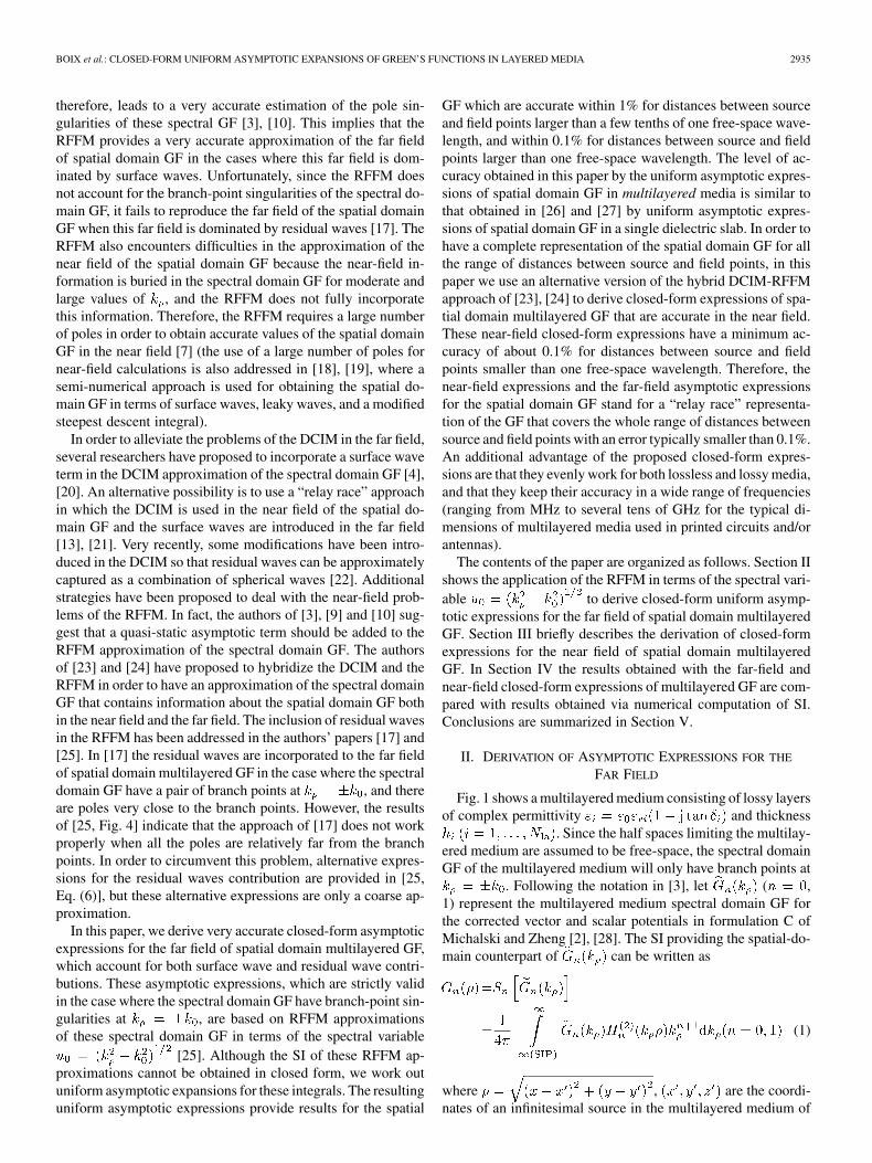
Fig. 1 shows a multilayered medium consisting of lossy layersof complex permittivity and thickness

. Since the half spaces limiting the multilay-ered medium are assumed to be free-space, the spectral domainGF of the multilayered medium will only have branch points at

. Following the notation in [3], let ( ,1) represent the multilayered medium spectral domain GF forthe corrected vector and scalar potentials in formulation C ofMichalski and Zheng [2], [28]. The SI providing the spatial-do-main counterpart of can be written as

(1)

where , are the coordi-nates of an infinitesimal source in the multilayered medium of


Fig. 1. Multilayered lossy medium limited by free-space at the upper end, andlimited either by a PEC or by free-space at the lower end. The source and fieldpoints are arbitrarily located inside the multilayered medium.

Fig. 1, are the coordinates of an arbitrary field point inFig. 1, is the Hankel function of order and second kind[29], and SIP is the Sommerfeld integration path that detoursaround the poles and branch points of (see Fig. 3(a)).Although in principle and are also functions of

and , in this paper we will derive approximate closed-formexpressions of and for fixed values of and ,and we will ignore the dependence of and onand . If were required in a certain range of values of

and , it would be necessary to obtain a set of closed-formexpressions of for pairs of samples of and withinthe required range, and then perform interpolation among thesets of expressions for the pairs of samples as suggested in [30,Fig. 2].

As is well known, in the complex -plane the spectral do-main GF, , of the multilayered medium of Fig. 1 have apair of branch-point singularities , a finite numberof poles in the proper Riemann sheet, and an infinite number ofpoles in the improper Riemann sheet. However, when the spec-tral domain GF are defined in terms of the new spectral variable

, in the complex -plane the functionsbecome single valued functions of with an infinite number ofpoles and without branch points [25]. Bearing in mind this idea,in this paper we propose to approximate the functionsin the vicinity of (i.e., in the vicinity of inthe -plane) by means of the following pole-residue represen-tation (see [25, Eq. (3)] for a similar representation):

(2)

where and are polynomials in the vari-able of degrees and , respectively. In this paper thecoefficients of these two polynomials are obtained by means ofthe total least squares algorithm (TLSA) [31] as explained in[3, Eqs. (8)–(10)], and the coefficients and ( , 1;

) are subsequently obtained in terms of the co-efficients of the polynomials as explained in [3, Eq. (12)]. Thesamples required for the application of the TLSA are chosen inthe -plane along the paths and of Fig. 2(a). These twopaths and map into an ellipse in the -plane detouringaround the branch point , around the proper poles, andaround the improper poles that are closest to the branch point

. The lower half of the ellipse (mapped by ) is placed

Fig. 2. Paths chosen in the complex � -plane (a) and the complex � -plane (b)when applying the total least squares algorithm to Eq. (2). The upper half-ellipseof (b) (solid line) is located in the proper Riemann sheet, and the lower half-ellipse of (b) (dashed line) is located in the improper Riemann sheet. � �� where � � �� .

in the improper Riemann sheet of the -plane, and the upperhalf of the ellipse (mapped by ) is placed in the proper Rie-mann sheet (see [25] for details).

In the results Section we will show that (2) provides an ex-tremely accurate approximation of on the paths and

of Fig. 2(a). In fact, (2) not only provides a very accurateapproximation of in the vicinity of but also pro-vides a very accurate approximation of in the vicinity ofthe branch points , in the vicinity of the proper poles,and in the vicinity of the improper poles which are closest tothe branch points. As a consequence of this, the spatial domaincounterpart of (2) should yield a very accurate approximationof the far field of [25].

When the approximation of (2) is introduced in (1), we obtainthe following approximate expression for :

(3)

where ( , 1; ) are integrals given by

(4)

Before proceeding with the calculation of , we will sortthe poles of (2) into three types.

• Type 1: poles for which . These poles map intopoles placed on the proper sheet of thecomplex -plane [see Fig. 3(a) and (b)].

• Type 2: , , and. These poles map into poles of the

improper sheet of the complex -plane which are placedinside the shadowed region of Fig. 3(b).

• Type 3: , oror . These


Fig. 3. (a) Deformation of the Sommerfeld integration path SIP to the paths�and � (all proper poles are captured in the deformation). (b) Deformation ofthe path � to the paths � and � (all type 2 improper poles are captured inthe deformation).

poles map into poles of the improper sheet of the complex-plane which are placed outside the shadowed region of

Fig. 3(b).Bearing in mind the definition of the three types of poles, the

integration path SIP of (4) can be deformed into the pathsand of Fig. 3(a), and can be further deformed into thepaths and of Fig. 3(b) (see also [17, Figs. 2 and 3]). As aresult of the integration paths deformations, the integrals of (4)can be rewritten as

(5)

where for poles of the type 1 and type 2, forpoles of the type 3, and ( , 1; ) arenew integrals given by

(6)

The Hankel functions of (5) are surface waves that repre-sent the contribution of the approximation of (2) to the discretespectrum of , and the integrals of (6) are residual wavesthat represent the contribution of the approximation of (2) tothe continuous spectrum of [17]. The integrals in(5) cannot be obtained in closed form. However, we should re-mind that the approximation of (2) is likely to provide an accu-rate approximation of the far field of , and therefore, weshould only be interested in the asymptotic expression offor large values of . In order to obtain that asymptotic expres-

sion, we introduce the change of variables in (6)[17], [32]. After this transformation, the integrals can berewritten as

(7)

where

(8)

(9)

and where the functions ( , 1) are given by

(10)

Since the functions are regular functions of , Pauli-Clemmow method can be used to carry out a uniform asymptoticexpansion of the integrals of (7) for large [33], [34]. In order toobtain the asymptotic expansion, the functions ( ,1) are first expanded in Taylor series in the neighborhood of

as shown below

(11)

After (11) is substituted in (7), the following uniform asymptoticexpansion of is obtained:

(12)

where

(13)

are integrals that can be obtained in closed form in terms ofthe error function (see [35, Appendix II]). In Appendix A weprovide expressions for ( , 1) and ( ,1; ) in the range .

Numerical simulations have shown that in the case where, the functions and of (12) can

be substituted by their asymptotic expressions for large , andin that case, the uniform asymptotic expansion of (12) adoptsthe simplified expression

(14)

In Appendix B we provide expressions for the coefficients( , 1; ) in the range .

III. EXPRESSIONS FOR THE NEAR FIELD

In the next Section we will check that (3), (5), (12), and (14)can be used to compute the far field of with an error


Fig. 4. Paths � and � used in the complex � -plane for the two-levelapplication of the discrete complex image method. If the source point isembedded in the �th layer of the multilayered medium of Fig. 1, then� � �� .

smaller than 0.1% when (provided ). Thus,in order to have closed-form approximations of that arevalid for all values of within a reasonable accuracy, we needadditional approximations of the near field of that areaccurate enough when . Bearing in mind the suggestionsof [3], [17] and [23], we propose to use near-field closed-formexpressions of that can be written in the spectral domainas

(15)

The functions of (15) stand for the asymptotic behaviorof for large values of [3]. Their spatial counter-parts, , contain the singularity of the source in thelimit and the first images of this static singularitythrough the interfaces of the layer containing the source. Allthe functions can be expressed as linear combinationsof functions of the type shown in [3, Eqs. (44) and (46)], andtheir closed-form spatial counterparts can be obtained as shownin [3, Eqs. (45) and (47)]. The functions and

of (15) are first and second level exponentialapproximations of that are ob-tained by means of the DCIM [6, Eq. (27)]. The amplitudesand exponents of the exponential functions and

are obtained via the GPOF, and the samples ofare computed in the paths and of Fig. 4 respectively.

The reasons for sampling in and are that onlyhave relevant values in the interval of thereal axis of the complex -plane, and that cannot beappropriately approximated by exponentials via the DCIM inthe interval since all the proper poles of

are placed in the vicinity of this interval (and theseproper poles cannot be reproduced by the “poles-free” expo-nentials of the DCIM). The functions of (15) con-tain the contribution to of the two proper poles( , 1) which are closest to the two branch points

[17, Eqs. (32) and (36)]. This contribution must be explic-itly included in the approximation of because the poles

are difficult to capture [17], especially when they are veryclose to the branch points [25, Sect. III]. The poles andtheir residues can be determined with a great accuracy when theTLSA is applied to (2) for far-field calculations [25]. Finally,the functions of (15) are pole-residue approxima-tions of

in terms of the spectral variable [3, Eq. (6)]. The

Fig. 5. Magnitude of the maximum relative error along the path of Fig. 2(a) inthe total least squares approximation of � via Eq. (2). The maximum relativeerror is plotted versus the number of pole-residue terms retained in (2). Theresults are presented for the multilayered medium of Fig. 1 (PEC at the bottom):� � �� , � � �� , � � �, � � � ��, � � �� ,� � ��, � � ��, � ��, � � ��, � ��, � ��,�� .

poles and residues of are determined via the TLSAdescribed in [3], and the samples of are computed in the path

of [3, Eq. (11)] along the interval .

IV. NUMERICAL RESULTS

In Fig. 5 we show the values of the maximum relative errorobtained along the paths and of Fig. 2(a) between theexact spectral domain scalar potential GF of a multilayeredmedium and the approximate spectral GF provided by thepole-residue representation of (2). The relative errors areplotted versus the number of terms used in (2) for twodifferent frequencies. Please note that maximum relative errorsbetween and are achieved when a sufficiently largevalue of is used. These maximum errors are substantiallysmaller than those obtained with the pole-residue representa-tions of [3, Eq. (6)] and [17, Eq. (38)] in the -plane, whichtypically range between 0.01% and 1% (e.g., see [3, Fig. (5)]).Therefore, Fig. 5 proves that the application of the RFFM inthe -plane leads to more accurate approximations than theapplication of the RFFM in the -plane. Fig. 5 also shows thatthe number of terms required in (2) to obtain a good accuracyincreases with increasing frequency. This is due to the fact that,as frequency increases, there is also an increase in the numberof proper poles of and in the number of improper polesof located in close proximity to the branch points.Therefore, as frequency increases, more poles are required in(2) for an accurate approximation of along the paths

and .In Figs. 6 and 7 we present numerical integration results

for (6) in two particular cases: an “improper” pole far fromthe origin of the -plane (which maps into improper polesof the complex -plane located far from the branch points)and an “improper” pole close to the origin of the -plane(which maps into improper poles of the complex -planelocated close to the branch points). We compare these resultswith those obtained with (12) and (14) in the cases ,


Fig. 6. Magnitude of the integral � of (6) in the case where � �� (“improper” pole far from the origin of the� -plane). This pole appears in the total least squares approximation of �for the structure studied in Fig. 5 when � � �� . Numerical integrationresults (solid line) are compared with those obtained by means of Eqs. (12)[Fig. 6(a)] and (14) [Fig. 6(b)] ��. The relative errors between numer-ical integration results and the approximate formulas of (12) and (14) are alsoplotted (dots and dashes, and dotted lines).

, and . Figs. 6(a) and 7(a) show that (12)provides with an error smaller than 0.1% when( is the free-space wavelength) and . Thisgives an estimation of the level of accuracy that we can reachwith (3), (5), and (12) in the approximation of thefar field of . Note that the errors plotted in Figs. 6(a)and 7(a) for the different values of show a decay of thetype as increases, which is to be expected as higherorder terms are successively retained in the uniform asymptoticexpansion of . Although we could have obtained resultsfor in Figs. 6(a) and 7(a), these two figures seem toindicate that this would have reduced the errors in the far-fieldestimation of but would have kept the errors in thenear field. Since the level of error obtained in the far fieldwith (smaller than 0.1% when ) suffices forpractical purposes, in the rest of this paper we will always workwith . Figs. 6(b) and 7(b) show the results obtainedwith (14), and the errors made with (14) in the estimation of

. Note that whereas the accuracy of (14) is similar to that

Fig. 7. Magnitude of the integral � of (6) in the case where � �� (“improper” pole close to the origin of the � -plane). Thispole appears in the total least squares approximation of � for the structurestudied in Fig. 5 when � � �� . Numerical integration results (solidline) are compared with those obtained by means of Eqs. (12) [Fig. 7(a)] and(14) [Fig. 7(b)] ��. The relative errors between numerical integrationresults and the approximate formulas of (12) and (14) are also plotted (dots anddashes, and dotted lines).

of (12) when [Fig. 6(b)], the accuracy of (14) canbecome very poor when [Fig. 7(b)]. Since themathematical expression of (14) is much simpler than that of(12), (14) should be always used when and (12)should be used when . Numerical simulations haveshown that when the TLSA is applied to (2), at least two-thirdsof the poles fulfill the condition , and (14) canbe safely applied to the calculation of for all thesepoles. In [25] we proposed to use a simplified version of (14)for all the poles which are not in close proximity to thebranch points of (specifically, for the poles fulfillingthe condition ). In the followingresults we will show that the values of the far field ofthat are obtained with the approach presented in this paper aremore accurate than those obtained via the approach of [25].

In Figs. 8 to 10 we plot the numerical results obtained for thespatial domain GF of different multilayered media by means of(3), (5), (12), and (14) when (these results are expectedto be accurate in the the far-field region). In all these figures, our


numerical results are compared with numerical integration re-sults obtained with either the weighted average method [1], [36]or the complex plane numerical integration technique describedin [37]. Please note that the errors between the results providedby the far-field expressions of Section II and the numerical inte-gration results are always basically below 0.1% when ,which agrees with the accuracy provided by (12) and (14) when

[see Fig. 6(a), (b), and 7(a)]. Also, in Figs. 8 to 10most of the relative-error curves provided by the present ap-proach show a decay of the type as increases, whichagrees with the slope observed for the errors in the logarithmicplots of Figs. 6(a), (b), and 7(a) when .

In Fig. 8(a)–(c) we present results for the component ofthe vector potential GF. The numerical results obtained with thefar-field expressions of (3) are compared with the results ob-tained with the far-field expressions of [25, Eq. (4)], and withnumerical integration results. Three different frequencies areconsidered. At , the spectral domain GF hasno proper poles and the improper poles are relatively far fromthe branch points. At , still has no properpoles, but it has two improper poles that are very close to thebranch points . Finally, at , has twoproper poles and all the poles (proper and improper) are againrelatively far from the branch point. Owing to this different lo-cation of the poles of , at the far field ofis dominated by a residual wave with a decay of the type ,at the far field of is dominated by a residualwave with a decay of the type that transitions to a decay ofthe type , and at the far field of is dom-inated by a damped surface wave that transitions to a residualwave with a decay of the type [17]. Fig. 8(a) to (c) show thatall these far-field scenarios are captured by (3) with amazing ac-curacy. In contrast, the far-field expressions of [25] lead to errorssuperior to 1% in wide ranges of , especially atand . This indicates that even though the resultsobtained with both (3) and [25, Eq. (4)] overlap the numericalintegration results at first glance, the far-field expressions ob-tained in Section II of this paper are clearly more reliable thanthose obtained in [25].

Next, Fig. 9(a)–(c) show results for the scalar potential GF.As expected, in Fig. 9(a) and (b) the errors between the resultsof (3) and numerical integration results decrease with increasing

(with a slope of 3 in the logarithmic plots) until either ma-chine roundoff errors or limitations in numerical integration ac-curacy cause the errors to stop decreasing. However, the errorsof Fig. 9(c) do not follow this behavior. On the one hand, thereare error peaks which coincide with the peaks of . Theselatter peaks are originated by interferences between two dampedsurface waves. On the other hand, the errors decrease until theyreach a stagnation level of 0.01%, which is larger than thoseobserved in Fig. 9(a) and (b). The larger errors of Fig. 9(c) areattributed to the loss of accuracy of the TLSA algorithm withincreasing frequency. As commented in [25], the TLSA stopsproviding accurate values of the poles and residues of(2) when . For frequencies above the thresholdfrequency of validity of the TLSA, the values of and sup-plied by (2) will cause that (3) provides unreasonable values ofthe far field of . As shown in Fig. 9(a) to (c), the closer the

Fig. 8. Magnitude of the spatial-domain GF � for a lossy four-layeredmedium of the type shown in Fig. 1 (PEC at the bottom). (a) � � �� , (b)� � ��, (c) � � ��. Numerical integration results (solid line) arecompared with those obtained via Eq. (3) �� and with those obtained via [25,Eqs. (4)–(6)] ��. The relative errors between numerical integration results andthe results of (3) and [25] are also plotted (dots and dashes, and dotted line). Pa-rameters of the multilayered media: � � �� , � � �� , � � ,� � �� , � � �� , � � �� , � � �� , � � ��,� � ��, � � ��, � � ��, �� ,�� . Parameter of the TLSA: � � ��.

frequency to the threshold frequency, the larger the errors of (3)will be. However, this does not invalidate the theory presentedin Section II for the computation of the far field of multilayered


Fig. 9. Magnitude of the spatial-domain GF � for a lossy four-lay-ered medium of the type shown in Fig. 1 (free-space at the bottom). (a)� � �� , (b) � � � ��, (c) � � �� . Numerical integra-tion results (solid line) are compared with those obtained via Eq. (3) �.The relative errors between numerical integration results and the results of(3) are also plotted (dashed line). Parameters of the multilayered media:� � �� , � � �� , � � , � � �� , � � �� ,� � �� , � � �� , � � ��, � � ��, � � ��,� � ��, �� , �� . Parameters of theTLSA: (a) � � �; (b) � � �; (c) � � ��.

GF. For frequencies above the threshold frequency of validityof the TLSA, one should use an alternative method for the com-putation of the poles and residues of (2) such as the VECTFIT

Fig. 10. Magnitude of the spatial-domain GF � for a lossless four-layeredmedium of the type shown in Fig. 1 (PEC at the bottom). (a) � � �� ,(b) � � � ��, (c) � � � ��. Numerical integration results (solid line)are compared with those obtained via Eq. (3) �. The relative errors betweennumerical integration results and the results of (3) are also plotted (dashed line).Parameters of the multilayered media: � � � � �, � � , � � �� ,� � �� , � � �� , � � �� , � � ��, � � ��,� � ��, � � ��, �� . Parametersof the TLSA: (a) � � �; (b) � � �; (c) � � ��.

algorithm described in [38]. Once and are computed withsufficient accuracy, (3)to (14) can still be used for the accurateasymptotic determination of the far field of multilayered GF.


Anyway, we would like to point out that the condition requiredfor the validity of the TLSA is satisfied bymost of the multilayered substrates used in planar circuits andprinted antennas in practice.

In Fig. 10(a)–(c) we present results for the component ofthe vector potential GF in order to show that the approach ofSection II not only works for the derivation of the far field ofSI of order 0 (see Figs. 8 and 9) but also works for the deriva-tion of the far field of SI of order 1. The behavior of the error inFig. 10(a)–(c) is very similar to that observed in Fig. 9(a)–(c).At low and intermediate frequencies ( and

) the error decreases below , and at high frequen-cies the error decreases until it stagnates be-tween and . Again, these differences are attributed tothe loss of accuracy of the TLSA as frequency increases. Themultilayered medium used in Fig. 10(a)–(c) is lossless, and thiscauses that the far field in these figures is dominated by surfacewaves. At and , only one surfacewave can be excited along the medium and the far field showsthe typical decay of the type . At the farfield consists of the interference among three surface waves. Allthese different far-field scenarios are again correctly reproducedby (3).

In Figs. 11 and 12 we present results for the near fields ofthe spatial domain GF plotted in Figs. 9 and 10. In particular,we plot the results obtained for the near field with the spatialcounterparts of (15), and we compare these results with numer-ical integration results. The errors between the results providedby (15) and numerical integration results are always basicallybelow 0.1% when . This indicates that the spatial coun-terparts of (15) provide robust and accurate expressions for thedetermination of the near field of spatial domain multilayeredGF, and therefore, they are complementary to (3), (5), (12), and(14). The data in the captions of Figs. 11 and 12 indicate thatthe number of DCIM terms required in (15) decreases with in-creasing frequency. This is due to the fact that the length of theinterval where the DCIM is applied, , decreaseswith increasing frequency, and therefore, the number of expo-nentials required in that interval also decreases with increasingfrequency. The opposite holds for the number of TLSA termsrequired in (15). As frequency increases, there is an increase inthe number of proper and improper poles placed in the neigh-borhood of the interval where the TLSA isapplied, and therefore, more pole-residue terms are required byTLSA approximation in that interval.

In Table I(a) and (b) we present the ratios between theCPU times required by numerical integration [37] and thoserequired by both (3) and the spatial counterpart of (15) in thecomputation of and at two different frequencies. Inthe determination of the near field results, the GF have beenregularly sampled along the interval . Inthe case of the far field results, the GF have been regularlysampled along the interval . A minimumaccuracy of three significant figures has been always requiredin the numerical integration results. Note that in the caseof the near field results at low frequencies, the CPU timesrequired by numerical integration are very short, and onlydiffer from those required by the closed-form expressions in

Fig. 11. Magnitude of the spatial-domain GF � for a lossy four-layeredmedium of the type shown in Fig. 1 (free-space at the bottom). (a) � � ��,(b) � � � ��, (c) � � �� . Numerical integration results (solid line)are compared with those obtained via the spatial counterpart of (15) �. Therelative errors between numerical integration results and the results providedby (15) are also plotted (dashed line). Parameters of the multilayered media asin Fig. 9. Parameters of the DCIM and TLSA: (a) � � �, � � �,� � �; (b) � � , � � �, � � �; (c) � � �,� � �, � � � .

about one order of magnitude. However, in the rest of thecases, the CPU times required by numerical integration aretypically three orders of magnitude longer than those requiredby the closed-form expressions. We have also obtained theCPU times required in the computation of and by


Fig. 12. Magnitude of the spatial-domain GF � for a lossless four-layeredmedium of the type shown in Fig. 1(a) (PEC at the bottom). (a) � � �� ,(b) � � � ��, (c) � � ��. Numerical integration results (solid line)are compared with those obtained via the spatial counterpart of (15) ��. Therelative errors between numerical integration results and the results provided by(15) are also plotted (dashed line). Parameters of the multilayered media as inFig. 10. Parameters of the DCIM and TLSA: (a) � � , � � ,� � ��; (b)� � �,� � ,� � �; (c)� � ,� � , � � ��.

the weighted average method [1], [36], and they have turnedout to be usually longer than those required by the numericalintegration method described in [37].

TABLE ICPU TIME RATIOS IN THE CALCULATION OF THE GF � OF FIG. 9 AND

� OF FIG. 10. THE RATIOS ARE BETWEEN THE CPU TIME REQUIRED

BY NUMERICAL INTEGRATION [37] AND THE CPU TIME REQUIRED BY THE

SPATIAL COUNTERPART OF (15) (NEAR FIELD), AND BETWEEN THE CPU TIME

REQUIRED BY NUMERICAL INTEGRATION [37] AND THE CPU TIME REQUIRED

BY (3) (FAR FIELD). (a) NEAR FIELD; (b) FAR FIELD

V. CONCLUSIONS

The authors have presented a novel approach for the deriva-tion of closed-form expressions of spatial domain multilayeredGF that are valid in the far field. The approach is based on a uni-form asymptotic expansion of the SI for the total least squaresapproximation of the spectral domain multilayered GF in termsof the spectral variable . The far-field asymp-totic expressions have proven to be accurate within 0.1% for dis-tances between source and field points larger than one free-spacewavelength. Also, the authors have demonstrated that the hy-brid use of both the discrete complex image method and the ra-tional function fitting method, which are very well establishedtechniques, makes it possible to derive near-field closed-formexpressions of the GF that are typically accurate within 0.1%for distances between source and field points smaller than onefree-space wavelength. Therefore, the combination of the novelfar-field expressions with the well-known near-field expressionsprovides an accurate "relay race" representation of the spatialdomain multilayered GF in the whole range of distances be-tween source and field points. The transition point between thefar-field and the near-field expressions is for a distance betweensource and field points of one free-space wavelength. Finally,it should be pointed out that the present approach works effi-ciently in the case of both lossless and lossy substrates, and fora wide range of frequencies that covers most of the situationsencountered in practice.

APPENDIX A

In this Appendix, we provide expressions for the functions( , 1) and ( , 1; ) of

(12) and (13) in the range

(16)

(17)


(18)

(19)

(20)

(21)

(22)

(23)

(24)

where and are given by

(25)

(26)

where is the error function [29]. In the expressions( , 1; ; , 2) of (25) and

(26), the plus sign must be chosen when andthe minus sign must be chosen when .

APPENDIX B

In this Appendix, we provide expressions for the coefficients( , 1; ) of (14) in the range :

(27)

(28)

(29)

(30)

(31)

(32)

ACKNOWLEDGMENT

The authors would like to express their gratitude to the re-viewers for their contributions to enhance the final quality ofthe paper.

REFERENCES

[1] J. R. Mosig, “Integral equation technique,” in Numerical Techniques forMicrow. and Millimeter-Wave Passive Structures, T. Itoh, Ed. NewYork: Wiley, 1989, pp. 133–213.

[2] K. A. Michalski and J. R. Mosig, “Multilayered media Green’sfunctions in integral equation formulations,” IEEE Trans. AntennasPropag., vol. 45, pp. 508–519, Mar. 1997.

[3] R. R. Boix, F. Mesa, and F. Medina, “Application of total least squaresto the derivation of closed-form Green’s functions for planar layeredmedia,” IEEE Trans. Microw. Theory Tech., vol. 55, pp. 268–280, Feb.2007.

[4] Y. L. Chow, J. J. Yang, D. G. Fang, and G. E. Howard, “A closed-formspatial Green’s function for the thick microstrip substrate,” IEEE Trans.Microw. Theory Tech., vol. 39, pp. 588–592, Mar. 1991.

[5] M. I. Aksun, “A robust approach for the derivation of closed-formGreen’s functions,” IEEE Trans. Microw. Theory Tech., vol. 44, pp.651–658, May 1996.

[6] P. Yla-Oijala and M. Taskinen, “Efficient formulation of closed-formGreen’s functions for general electric and magnetic sources in multilay-ered media,” IEEE Trans. Antennas Propag., vol. 51, pp. 2106–2115,Aug. 2003.

[7] V. I. Okhmatovski and A. C. Cangellaris, “A new technique for thederivation of closed-form electromagnetic Green’s functions for un-bounded planar layered media,” IEEE Trans. Antennas Propag., vol.50, pp. 1005–1016, July 2002.

[8] A. G. Polimeridis, T. V. Yioultsis, and T. D. Tsiboukis, “Fast numer-ical computation of Green’s functions for unbounded planar stratifiedmedia with a finite-difference technique and Gaussian spectral rules,”IEEE Trans. Microw. Theory Tech., vol. 55, pp. 100–107, Jan. 2007.

[9] V. I. Okhmatovski and A. C. Cangellaris, “Evaluation of layered mediaGreen’s functions via rational function fitting,” IEEE Microw. WirelessCompon. Lett., vol. 14, pp. 22–24, Jan. 2004.

[10] V. N. Kourkoulos and A. C. Cangellaris, “Accurate approximation ofGreen’s functions in planar stratified media in terms of a finite sum ofspherical and cylindrical waves,” IEEE Trans. Antennas Propag., vol.54, pp. 1568–1576, May 2006.

[11] F. Ling, V. Okhmatovski, B. Song, and A. Dengi, “Systematic extrac-tion of static images from layered media Green’s function for accurateDCIM implementation,” IEEE Antennas Wireless Propag. Lett., vol. 6,pp. 215–218, 2007.

[12] N. V. Shuley, R. R. Boix, F. Medina, and M. Horno, “On the fastapproximation of Green’s functions in MPIE formulations for planarlayered media,” IEEE Trans. Microw. Theory Tech., vol. 50, pp.2185–2192, Sep. 2002.

[13] M. I. Aksun and G. Dural, “Clarification of issues on the closed-formGreen’s functions in stratified media,” IEEE Trans. Antennas Propag.,vol. 53, pp. 3644–3653, Nov. 2005.

[14] M. Yuan, T. K. Sarkar, and M. Salazar-Palma, “A direct discretecomplex image method from the closed-form Green’s functions inmultilayered media,” IEEE Trans. Microw. Theory Tech., vol. 54, pp.1025–1032, Mar. 2006.


[15] L. Zhuang, G. Zhu, Y. Zhang, and B. Xiao, “An improved discretecomplex image method for Green’s functions in multilayered media,”Microw. Opt. Technol. Lett., vol. 49, no. 6, pp. 1337–1340, June 2007.

[16] F. J. Demuynck, G. A. E. Vandenbosch, and A. R. Van de Capelle,“The expansion wave concept—Part I: Efficient calculation of spatialGreen’s functions in a stratified dielectric medium,” IEEE Trans. An-tennas Propag., vol. 46, pp. 397–406, Mar. 1998.

[17] F. Mesa, R. R. Boix, and F. Medina, “Closed-form expressions of mul-tilayered planar Green’s functions that account for the continuous spec-trum in the far field,” IEEE Trans. Microw. Theory Tech., vol. 56, pp.1601–1614, Jul. 2008.

[18] L. Tsang and B. Wu, “Electromagnetic fields of Hertzian dipoles in lay-ered media of moderate thickness including the effects of all modes,”IEEE Antennas Wireless Propag. Lett., vol. 6, pp. 316–319, Jun. 2007.

[19] B. Wu and L. Tsang, “Fast computation of layered medium Green’sfunctions of multilayers and lossy media using fast all-modes methodand numerical modified steepest descent path method,” IEEE Trans.Microw. Theory Tech., vol. 56, pp. 1446–1454, Jun. 2008.

[20] S.-A. Teo, S.-T. Chew, and M.-S. Leong, “Error analysis of the dis-crete complex image method and pole extraction,” IEEE Trans. Mi-crow. Theory Tech., vol. 51, pp. 406–413, Feb. 2003.

[21] C. H. Chan and R. A. Kipp, “Application of the complex image methodto multilevel, multiconductor microstrip lines,” Int. J. Microw. Milli.Comput. Aided Eng., vol. 7, pp. 359–367, 1997.

[22] M. I. Aksun, A. Alparslan, and K. A. Michalski, “Current status ofclosed-form Green’s functions in layered media composed of naturaland artificial materials,” in Proc. Int. Conf. on Electromagnetics in Ad-vanced Applications, Torino, Italy, Sep. 2009, pp. 451–454.

[23] A. G. Polimeridis, T. V. Yioultsis, and T. D. Tsiboukis, “A robustmethod for the computation of Green’s functions in stratified media,”IEEE Trans. Antennas Propag., vol. 55, pp. 1963–1969, Jul. 2007.

[24] A. G. Polimeridis and T. V. Yioultsis, “On the efficient computationof closed-form Green’s functions in planar stratified media,” Int. J. RFMicrow. Comput. Aided Eng., vol. 18, no. 2, pp. 118–126, Mar. 2008.

[25] A. L. Fructos, R. R. Boix, R. Rodríguez-Berral, and F. Mesa, “Efficientdetermination of the poles and residues of spectral domain multilay-ered Green’s functions that are relevant in far-field calculations,” IEEETrans. Antennas Propag., vol. 58, pp. 218–222, Jan. 2010.

[26] M. Marin, S. Barkeshli, and P. Pathak, “Efficient analysis of planarmicrostrip geometries using a closed-form asymptotic representationof the grounded dielectric slab Green’s function,” IEEE Trans. Microw.Theory Tech., vol. 37, pp. 669–679, Apr. 1989.

[27] S. Barkeshli, P. H. Pathak, and M. Marin, “An asymptotic closed-formmicrostrip surface Green’s function for the efficient moment methodanalysis of mutual coupling in microstrip antennas,” IEEE Trans. Mi-crow. Theory Tech., vol. 38, pp. 1374–1383, Sep. 1989.

[28] K. A. Michalski and D. Zheng, “Electromagnetic scattering and radi-ation by surfaces of arbitrary shape in layered media, part I: Theory,”IEEE Trans. Antennas Propag., vol. 38, pp. 335–344, Mar. 1990.

[29] M. Abramowitz and I. Stegun, Handbook of Mathematical Functions,9th ed. New York: Dover, 1970.

[30] C. H. Chan and R. A. Kipp, “Application of the complex image methodto characterization of microstrip vias,” Int. J. Microw. Milli. CAE, vol.7, no. 5, pp. 368–379, 1997.

[31] S. V. Huffel and J. Vandevalle, The Total Least Squares Problem: Com-putational Aspects and Analysis. Philadelphia: SIAM, 1991, vol. 9,Frontiers in Applied Mathematics.

[32] P. Baccarelli, P. Burghignoli, F. Frezza, A. Galli, G. Lovat, and D. R.Jackson, “Approximate analytical evaluation of the continuous spec-trum in a substrate-superstrate dielectric waveguide,” IEEE Trans. Mi-crow. Theory Tech., vol. 50, pp. 2690–2701, Dec. 2002.

[33] C. Gennarelli and L. Palumbo, “A uniform asymptotic expansion of atypical diffraction integral with many coalescing simple pole singular-ities and first-order saddle point,” IEEE Trans. Antennas Propag., vol.32, pp. 1122–1124, Oct. 1984.

[34] R. Rojas, “Comparison between two asymptotic methods,” IEEETrans. Antennas Propag., vol. 35, pp. 1489–1492, Dec. 1987.

[35] P. Baccarelli, P. Burghignoli, F. Frezza, A. Galli, G. Lovat, and D.R. Jackson, “Uniform analytical representation of the continuousspectrum excited by dipole sources in a multilayer dielectric structurethrough weighted cylindrical leaky waves,” IEEE Trans. AntennasPropag., vol. 52, pp. 653–665, Mar. 2004.

[36] J. R. Mosig and F. E. Gardiol, “Analytical and numerical techniques inthe Green’s function treatment of microstrip antennas and scatterers,”Proc. Inst. Elect. Eng., vol. 130, no. 2, pt. H, pp. 175–182, 1983.

[37] J. R. Mosig and A. álvarez-Melcón, “Green’s functions in lossy layeredmedia: Integration along the imaginary axis and asymptotic behavior,”IEEE Trans. Antennas Propag., vol. 51, pp. 3200–3208, Dec. 2003.

[38] B. Gustavsen and A. Semlyen, “Rational approximation of frequencydomain responses by vector fitting,” IEEE Trans. Power Delivery, vol.14, pp. 1052–1061, July 1999.

Rafael R. Boix (M’96) received the Licenciado andDoctor degrees in physics from the University ofSeville, Spain, in 1985 and 1990, respectively.

Since 1986, he has been with the Electronics andElectromagnetism Department, University of Seville,where he became Associate Professor in 1994. Hiscurrent research interests are focused on the numer-ical analysis of periodic planar electromagnetic struc-tures with applications to the design of frequency se-lective surfaces and electromagnetic bandgap passivecircuits.

Ana L. Fructos received the Licenciado degree inphysics from the University of Seville, Spain, in2005, where she is currently working toward thePh.D. degree.

Mrs. Fructos was the recipient of a Scholarship fi-nanced by the Junta de Andalucía.

Francisco Mesa (M’93) was born in Cádiz, Spain,on April 1965. He received the Licenciado degree inJune 1989 and the Doctor degree in December 1991,both in physics, from the University of Seville, Spain.

He is currently Associate Professor in the Depart-ment of Applied Physic 1 at the University of Seville,Spain. His research interest focus on electromagneticpropagation/radiation in planar structures.

Date post:	25-Oct-2020
Category:	Documents
Upload:	others
View:	1 times
Download:	0 times

2934 IEEE TRANSACTIONS ON ANTENNAS AND PROPAGATION,...

Documents