1 of 19

2B.3 AN IMPROVED BULK AIR-SEA SURFACE FLUX ALGORITHM,

INCLUDING SPRAY-MEDIATED TRANSFER

Edgar L Andreas1*

, Larry Mahrt2, and Dean Vickers

3

1NorthWest Research Associates, Inc.; Lebanon, New Hampshire

2NorthWest Research Associates, Inc.; Corvallis, Oregon

3College of Earth, Ocean, and Atmospheric Sciences, Oregon State University; Corvallis, Oregon

1. INTRODUCTION

Heat and moisture can cross the air-sea interface by two routes. The interfacial route,

which is controlled by molecular processes right at

the air-sea interface, is the one implicitly treated in

virtually all turbulent air-sea bulk flux algorithms. The spray route, in which transfer is controlled by

microphysical processes around sea spray

droplets, becomes significant at modest wind

speeds of 10–13 m s–1

.

Andreas et al. (2008) published our first

publicly released version of a bulk air-sea flux

algorithm that explicitly treats both the interfacial

and spray routes for the air-sea sensible and

latent heat fluxes. Andreas (2010) later added

comparable parameterizations for the enthalpy,

salt, and freshwater fluxes. These two algorithms

were denoted, respectively, Version 3.2 and

Version 3.4.

Here, we introduce Version 4.0 of this bulk

flux algorithm. This version improves on previous

versions in two significant ways. In all previous

versions, we built the interfacial flux algorithm on

the COARE Version 2.6 algorithm (Fairall et al.

1996; see Perrie et al. 2005; Andreas et al. 2008).

As such, it obtained a drag coefficient from an

aerodynamic roughness length, z0, which it

modeled as a smooth blending of the Charnock

relation and an aerodynamically smooth tail in low

winds (Smith 1988). Our previous versions also

included the COARE gustiness parameterization

in unstable stratification and a windless term in

stable stratification (from Jordan et al. 1999;

Andreas et al. 2008). Both of these

parameterizations prevented the surface stress

and the scalar fluxes from going to zero when the

vector-averaged wind speed was zero.

*Corresponding author address: Dr. Edgar L

Andreas, NorthWest Research Associates, Inc.,

25 Eagle Ridge, Lebanon, NH 03766-1900; e-mail:

eandreas@nwra.com.

In Version 4.0, however, we introduce a

totally new drag relation (Andreas et al. 2012) that

naturally provides a non-zero surface stress even

at zero average wind speed and has better

properties than the Charnock relation when

extrapolated beyond winds of 30 m s–1

. Hence,

from Version 4.0, we can eliminate the gustiness

and windless terms at low wind speed and can

reliably extrapolate our algorithm to hurricane-

strength winds, where the Charnock relation had

previously predicted too much surface drag and,

thus, too much dissipation to sustain modeled

hurricanes.

The second significant improvement in

Version 4.0 is that we have validated and tuned it

with 10 times as much data as used in deriving

previous versions.

With this enhanced validation for wind speeds

up to almost 25 m s–1

, because both the interfacial

and spray flux algorithms are theoretically based,

and since the new drag relation is consistent with

theory for wind speeds up to at least 70 m s–1

, this

new flux algorithm can be extrapolated to

hurricane-strength winds. Although forecasts of

hurricane track have improved dramatically in the

last 15 years, forecasts of hurricane intensity have

improved little (e.g., Rogers et al. 2013). Because

air-sea exchange is generally believed to control

hurricane intensity (e.g., Montgomery et al. 2010;

Lee and Chen 2012), the improved predictions of

air-sea fluxes that our algorithm promises may

provide insights into this difficult problem of

predicting hurricane intensity.

2. FLUX CALCULATIONS

2.1. General Outline

As with most flux algorithms, ours provides

the “surface” fluxes of momentum (τ, also called

the surface stress), latent heat (HL), and sensible

heat (Hs):

2 of 19

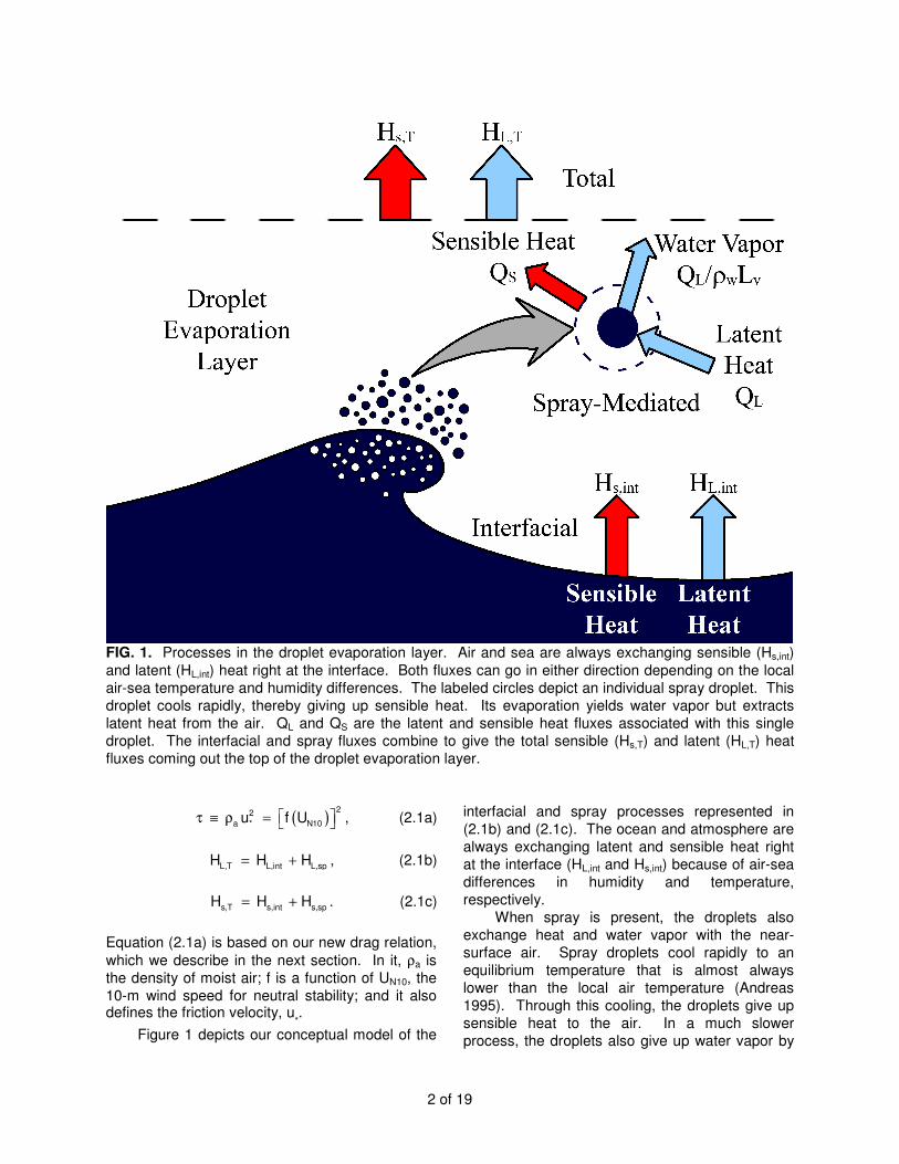
FIG. 1. Processes in the droplet evaporation layer. Air and sea are always exchanging sensible (Hs,int)

and latent (HL,int) heat right at the interface. Both fluxes can go in either direction depending on the local

air-sea temperature and humidity differences. The labeled circles depict an individual spray droplet. This

droplet cools rapidly, thereby giving up sensible heat. Its evaporation yields water vapor but extracts

latent heat from the air. QL and QS are the latent and sensible heat fluxes associated with this single

droplet. The interfacial and spray fluxes combine to give the total sensible (Hs,T) and latent (HL,T) heat

fluxes coming out the top of the droplet evaporation layer.

( )22

a * N10u f U τ ≡ ρ = , (2.1a)

L,T L,int L,spH H H= + , (2.1b)

s,T s,int s,spH H H= + . (2.1c)

Equation (2.1a) is based on our new drag relation,

which we describe in the next section. In it, ρa is

the density of moist air; f is a function of UN10, the

10-m wind speed for neutral stability; and it also defines the friction velocity, u

*.

Figure 1 depicts our conceptual model of the

interfacial and spray processes represented in

(2.1b) and (2.1c). The ocean and atmosphere are

always exchanging latent and sensible heat right

at the interface (HL,int and Hs,int) because of air-sea

differences in humidity and temperature,

respectively.

When spray is present, the droplets also

exchange heat and water vapor with the near-

surface air. Spray droplets cool rapidly to an

equilibrium temperature that is almost always

lower than the local air temperature (Andreas

1995). Through this cooling, the droplets give up

sensible heat to the air. In a much slower

process, the droplets also give up water vapor by

3 of 19

evaporating (Andreas 1990). Because the

droplets are now relatively cool, however, the

latent heat for this evaporation must come from

the air. As a consequence, this evaporation

enhances the interfacial flux of water vapor but

cools the near-surface atmosphere, thereby

offsetting some of the sensible heating contributed

when the droplets initially cooled.

These spray-mediated processes occur over

a range of droplet radii that is 1.6 to 500 µm in our

current analysis. Each droplet size has different

time scales for its exchanges of sensible and

latent heat. To get the spray-mediated fluxes in

(2.1b) and (2.1c), HL,sp and Hs,sp, we must combine

individual contributions with knowledge of how

many droplets are produced and integrate over all

radii. We describe that process shortly.

This spray-mediated transfer occurs in a

near-surface droplet evaporation layer (Figure 1)

that is nominally one significant wave height thick

(Andreas et al. 1995; Van Eijk et al. 2001).

Hence, the so-called surface fluxes in (2.1b) and

(2.1c) are what we denote as the total fluxes (HL,T

and Hs,T) that come out the top of the droplet

evaporation layer. These would serve as the

lower flux boundary conditions in atmospheric

models and be applied at the lowest modeling

node. Similarly, we assume that the measured

latent and sensible heat fluxes that we use to

validate and tune our algorithm were obtained

above the droplet evaporation layer and therefore

represent HL,T and Hs,T.

2.2. Drag Relation

Andreas et al. (2012) analyzed over 5600

eddy-covariance measurements of the air-sea

surface stress from ships, platforms, and aircraft.

This analysis confirmed the observations by Foreman and Emeis (2010) that u

* is a linear

function of UN10, the 10-m wind speed at neutral

stability, in aerodynamically rough flow over the

ocean (cf. Edson et al. 2013).

Andreas et al. (2012) also obtained a linear relation between u

* and UN10 for aerodynamically

smooth flow and were, therefore, able to connect

these two straight-line regions with a hyperbola that predicts u

* from UN10 for all wind speeds and

is a continuous and differentiable function. That

hyperbola, which is the f(UN10) function is (2.1a), is

( ) ( ){ }*

1/ 22

N10 N10

u 0.239 0.0433

U 8.271 0.120 U 8.271 0.181

= + •

− + − +

. (2.2)

Here, both u

* and UN10 are in m s

–1.

Figure 2 shows (2.2) and the data that

Andreas et al. (2012) used in deriving it. The

figure also shows theoretical results from Moon et

al. (2007) and Mueller and Veron (2009a). Both of

these theoretical studies extended to wind speeds

of at least 60 m s–1

, as depicted in the figure.

Because, beyond the range of our data, the

extrapolation of (2.2) agrees well with these two

theoretical results, we believe that extrapolating

(2.2) to hurricane-strength winds is consistent with

theory. The Charnock relation from previous

versions of our algorithm (Andreas et al. 2008; cf.

Fairall et al. 1996, 2003; see Figure 2) predicts

progressively increasing drag for UN10 above

30 m s–1

that is not compatible with the needs of

hurricane models.

The crucial feature of (2.2) that makes

extrapolating it meaningful is that in higher winds it

reduces to

* N10u 0.0583U 0.243= − , (2.3)

where u

* and UN10 are still in m s

–1. As such, for

higher winds, our hyperbola easily gives the more

familiar 10-m, neutral-stability drag coefficient:

2 2

3*DN10

N10 N10

u 4.17C 3.40 10 1

U U

− ≡ = × −

. (2.4)

That is, (2.2) predicts CDN10 to increase

monotonically with increasing wind speed but to

roll off to an asymptotic value of 33.40 10−× at very

high wind speeds.

As (2.2) and (2.4) do, limiting the value of the

drag coefficient in high winds to values much less

than those predicted by the Charnock relation, for

example, seems to have helped recent hurricane

models (e.g., Jarosz et al. 2007; Sanford et al.

2007; Chiang et al. 2011). In addition, for major

hurricane wind speeds of 60–75 m s–1

, (2.4) gives

CDN10 values near 33.0 10−× . Coincidentally, this is

the limiting value that Tang and Emanuel (2012)

imposed in their recent hurricane modeling study.

For completeness, we mention how we

calculate UN10 in our analysis or in implementing

our algorithm. We use (Andreas et al. 2012)

4 of 19

FIG. 2. Summary of the drag analysis in

Andreas et al. (2012). The black circles are

averages in UN10 bins 1 m s–1

wide. The error

bars are ±2 standard deviations in the bin

populations. The red circles are medians in

these same bins. The curves denote the

hyperbola (2.2), which is the drag relation in our

flux algorithm, and the theoretical results of

Moon et al. (2007) and Mueller and Veron

(2009a). The blue curve is the Charnock

relation from our previous algorithm (Andreas et

al. 2008).

( ) ( ) ( )*N10 m

uU U z ln z /10 z /L

k = − − ψ . (2.5)

Here, U(z) is the measured or modeled wind speed at height z (in meters); u

* is the

corresponding measured or modeled friction

velocity; k (= 0.40) is the von Kármán constant;

and ψm is the stratification correction for the wind

speed profile in the atmospheric surface layer, a

function of the Obukhov length, L. For ψm, we use

the function from Paulson (1970) in unstable

stratification, the function from Grachev et al.

(2007) in stable stratification, and

s L

3a p a v*

H Hz k zg 0.61T

L c LTu 1 0.61Q

= − + ρ ρ+

. (2.6)

In this, g is the acceleration of gravity; T and Q ,

the average air temperature and specific humidity

of the surface layer; cp, the specific heat of air at

constant pressure; and Lv, the latent heat of

vaporization. Depending on whether z/L is used in

our analysis or for model calculations, u*, Hs, and

HL represent either the measured u* and the total

measured fluxes, Hs,T and HL,T, or the modeled u*

and the modeled interfacial fluxes, Hs,int and HL,int.

2.3. Interfacial Flux Algorithm

With our new expression for the surface stress—now formulated in terms of u

* and UN10,

(2.1a) and (2.2)—our equations for the interfacial

heat fluxes differ from the common forms (cf.

Garratt 1992, pp. 54ff.; Fairall et al. 1996, 2003;

Perrie et al. 2005; Andreas et al. 2008) and are

( )

( ) ( )a v * s z

L,int

Q h

L ku Q QH

ln z / z z /L

ρ −=

− ψ, (2.7a)

( )

( ) ( )a p * s z

s,int

T h

c kuH

ln z / z z /L

ρ Θ − Θ=

− ψ. (2.7b)

In these, Qs and Θs are the specific humidity and

potential temperature at the sea surface, and Qz

and Θz are the humidity and temperature at height

z. ψh is the stratification correction for the scalar

profiles in the atmospheric surface layer; again,

we use the function from Paulson (1970) in

unstable stratification and the function from

Grachev et al. (2007) in stable stratification.

Finally, in (2.7), zQ and zT are the roughness

lengths for the humidity and temperature profiles.

We still use the COARE Version 2.6 expressions

for these (Fairall et al. 1996). Remember, Liu et

al. (1979) derived the zQ and zT algorithms in

Version 2.6 from surface renewal theory. We do,

however, limit zQ and zT to values greater than 87.0 10 m−× , approximately the mean free path of

air molecules (Andreas and Emanuel 2001).

As with most bulk flux algorithms, we solve

the system of equations (2.2) and (2.5)–(2.7) iteratively until u

*, Hs,int, and HL,int converge. This

iteration usually takes about three steps.

Notice in (2.1a), (2.2), (2.5), and (2.7) the

conspicuous absence of the aerodynamic

roughness length z0. Because our new drag

relation is formulated without z0, it avoids all of the

uncertainties in formulations of z0, including the

severe self-correlation in attempts to evaluate its

behavior from data (e.g., Mahrt et al. 2003).

5 of 19

2.4. Full Spray-Mediated Flux Model

Microphysical modeling demonstrates that,

under constant environmental conditions, the

temperature T and radius r of a sea spray droplet

evolve as functions of the time since formation t

approximately as (Andreas 1990, 2005; Andreas

and DeCosmo 1999, 2002)

( )

( )eq

T

s eq

T t Texp t /

T

−= − τ

Θ −, (2.8)

( )

( )eq

r

0 eq

r t rexp t /

r r

−= − τ

−. (2.9)

Here, Teq is the equilibrium temperature of a saline

droplet with initial radius r0 and initial temperature

Θs, the sea surface temperature; req is the

equilibrium radius of the same droplet; τT and τr

are the e-folding times that characterize the rates

of these exponential temperature and radius

changes. Realize that the temperature change

reflects the sensible heat transfer mediated by the

droplet while the radius change implies a flux of

water vapor and thus latent heat exchange.

In our data analysis, the values of Teq, req, τT,

and τr in (2.8) and (2.9) come from Andreas’s

(1989, 1990, 1992, 1995) full microphysical model.

Among other features, this model includes an

equation of state for estimating the solution

density of a spray droplet as it cools and

evaporates. Andreas (2005), however, developed

algorithms for quickly computing these

microphysical quantities; we use these fast

algorithms in the fast flux algorithm that we

describe later.

Briefly, all four microphysical quantities in

(2.8) and (2.9) depend on sea surface

temperature, air temperature, relative humidity,

sea surface salinity, barometric pressure, and

initial droplet radius. For typical ocean salinities of

34–35 psu, τT is about 5 s for the largest droplets

we consider, r0 = 500 µm, and is of order 10–4

s for

the smallest droplets, 1.6 µm. τr is typically three

orders of magnitude longer than τT. That is,

sensible heat exchange from spray droplets is

very fast while latent heat exchange is relatively

slow. See Figure 2 in Andreas and DeCosmo

(2002).

To put these time scales in perspective, we

also estimate the time scale for a droplet’s

residence in air:

( )

1/3f

f 0

H

2u rτ = . (2.10)

In this, uf(r0) is the terminal fall speed of droplets

with initial radius r0, and H1/3 is the significant wave

height. Because H1/3/2 is then the significant wave

amplitude, (2.10) reiterates our conceptual picture

(Andreas, 1992) that the droplets most important

for spray-mediated transfer are the large spume

droplets (Andreas, 2002) that originate at the wave

crests and fall ballistically back into the sea.

With (2.8)–(2.10), it is easy to estimate the

spray-mediated sensible and latent fluxes. The

spray sensible heat exchange facilitated by all

droplets of radius r0 is (Andreas 1992; Andreas et

al. 2008)

( ) ( )

( )

S 0 w w s eq

3

0f T

0

Q r c T

4 r dF1 exp /

3 dr

= ρ Θ −

π • − −τ τ

. (2.11)

In this, ρw is the density of seawater, and cw is its

specific heat. From (2.8), we see that

( ) ( )s eq f rT 1 exp / Θ − − −τ τ is the difference

between a droplet’s initial temperature and its

temperature when it falls back into the sea. This

temperature difference is related to the sensible

heat that droplets of radius r0 transfer.

The dF/dr0 in (2.11) is the spray generation

function, which gives the number of droplets of

initial radius r0 that are produced per square meter

of sea surface, per second, per micrometer

increment in droplet radius (e.g., Andreas 2002).

It thus has units of m–2

s–1

µm–1

. Hence,

( )3

0 04π r / 3 dF / dr is the rate at which the volume of

droplets of r0 is produced. Therefore, QS has units

of W m–2

µm–1

and estimates the rate of heat

transfer by all droplets of radius r0.

For dF/dr0, we use the function from Fairall et

al. (1994), as recommended in Andreas (2002).

Although there has been quite a bit of recent work

on the generation of film and jet droplets—see

de Leeuw et al. (2011) for a review—there has

been less work on the generation of spume

droplets. Spume is the most important droplet

class for spray-mediated transfer: see Figures 5–

8 in Andreas (1992) or Figure 2 in Andreas et al.

(2008). The recent papers by Mueller and Veron

(2009b), Fairall et al. (2009), and Veron et al.

(2012), nevertheless, do tend to corroborate the

6 of 19

general magnitude of the Fairall et al. (1994)

function.

As with (2.11), we estimate the latent heat

exchange associated with all droplets of radius r0

as

( )( )

33

f 0L 0 w v

0 0

r 4 r dFQ r L 1

r 3 dr

τ π = ρ −

. (2.12)

Here, r(τf) comes from (2.9) with τf substituted for t

and thus is the radius that droplets of initial radius

r0 have when they fall back into the sea. As such,

( ) ( ){ }33

w 0 f 04π / 3 r r dF / dr ρ − τ is the mass of

water that all droplets of initial radius r0 leave in

the air during their brief flights.

To get the total spray-mediated exchanges,

we must integrate (2.11) and (2.12) over all droplet

sizes:

( )500

S S 0 01.6Q Q r dr= ∫ , (2.13a)

( )500

L L 0 01.6Q Q r dr= ∫ . (2.13b)

These have units of a heat flux, W m–2

. The lower

and upper limits of radius integration, 1.6 and

500 µm, are the limits of validity of the Fairall et al.

(1994) spray generation function [see Andreas

(2002) for the equations to compute it].

Andreas and DeCosmo (1999, 2002) termed

SQ and LQ the nominal spray fluxes because

they hypothesized (also Andreas et al. 2008;

Andreas 2010) that the actual spray-mediated

latent and sensible heat fluxes are (cf. Fairall et al.

1994; Kepert et al. 1999)

LL,spH Q= α , (2.14a)

( )S Ls,spH Q Q= β − α − γ . (2.14b)

In these, α, β, and γ are presumed to be small,

positive tuning coefficients that we evaluate from

data. Although LQ and SQ are based on

microphysics and the dF/dr0 in them is constrained

by energy arguments (e.g., Andreas 2002), there

are some approximations and uncertain

parameters in these theories; dF/dr0 is one of the

largest sources of this uncertainty. Nevertheless,

because of their physical basis, LQ and SQ

correctly represent the dependencies of the fluxes

on environmental variables such as wind speed

(i.e., Andreas 2002; Andreas et al. 2008), air and

water temperatures, relative humidity, and ocean

salinity (Andreas 1990, 1995, 1996, 2005;

Andreas and Emanuel 2001). The α, β, and γ,

therefore, minimize the impact of these

uncertainties by letting us tune HL,sp and Hs,sp with

data, which we do shortly.

In (2.14a), α simply lets us adjust LQ to

agree with data. Similarly, in (2.14b), the β term is

the direct spray-mediated sensible heat exchange.

But, as Figure 1 depicts, because droplet

evaporation is slower than a droplet’s sensible

heat exchange, all of the LQα term in (2.14a)

must be supplied by the air in the droplet

evaporation layer. That is, droplet evaporation

consumes sensible heat, thereby cooling the air;

the LQα term in (2.14a) must thus appear with a

negative sign in (2.14b).

This cooling associated with the droplet’s

latent heat exchange occurs within the droplet

evaporation layer, which is typically below the

height z where Θz is specified in (2.7b). That is,

(2.7b) is unaware of these near-surface

temperature changes and would, thus,

underestimate Hs,int. See Figure 7 in Andreas et

al. (1995) or Figure 4 in Fairall et al. (1994). The

LQγ term in (2.14b) is meant to recognize the

steeper near-surface temperature gradient caused

by spray evaporation and, thus, adds an extra

sensible heat flux to augment the flux missed in

(2.7b).

3. DATA

The data that we use in our analysis are

some of the same sets that Mahrt et al. (2012),

Andreas et al. (2012, 2013), and Vickers et al.

(2013) have been using recently. Table 1 lists

these datasets. The key feature of all these data is that u

*, HL,T, and Hs,T were measured with eddy-

covariance instruments. Andreas et al. (2013)

review the instruments used for these

measurements.

Only the HEXOS and FASTEX sets include

measurements of significant wave height that we

need in (2.10). For all the other datasets, we

estimated H1/3 from Andreas and Wang’s (2007)

algorithm.

7 of 19

Table 1. The datasets used in this study. The “Number of Observations” is the number of cases left after

the screening described in the text. The “Reference” provides additional details on a dataset.

Dataset Number of

Observations Platform/Location Reference

CARMA4a

437 CIRPAS Twin Otter, off coast of southern California

Vickers et al. (2013)

CBLAST-weakb

2 Long-EZ aircraft, Martha’s Vineyard, Massachusetts

Edson et al. (2007)

FASTEXc

263 R/V Knorr, transect across the North Atlantic

Persson et al. (2005)

GFDexd

102 FAAM BAE 146 aircraft, Irminger Sea and Denmark Strait

Petersen and Renfrew (2009)

GOTEXe

817 NCAR C-130, Gulf of Tehuantepec

Romero and Melville (2010)

HEXOSf

173 Meetpost Noordwijk platform, North Sea

DeCosmo (1991), DeCosmo et al. (1996)

MABLEBg

40 CIRPAS Twin Otter, off Monterey, California

Vickers et al. (2013)

Monterey 556 CIRPAS Twin Otter, off Monterey, California

Mahrt and Khelif (2010)

POSTh

171 CIRPAS Twin Otter, off Monterey, California

Vickers et al. (2013)

REDi

351 CIRPAS Twin Otter, east of Oahu, Hawaii

Anderson et al. (2004)

SHOWEXj Nov ‘97 366 Long-EZ aircraft,

off coast of Virginia and North Carolina

Sun et al. (2001)

TOGA COAREk

742 NCAR Electra, western equatorial Pacific Ocean

Sun et al. (1996), Vickers and Esbensen (1998)

aCloud-Aerosol Research in the Marine Atmosphere, experiment 4.

bCoupled Boundary Layers and Air-Sea Transfer in weak winds.

cFronts and Atlantic Storm-Tracks Experiment.

dGreenland Flow Distortion experiment.

eGulf of Tehuantepec Experiment.

fHumidity Exchange over the Sea experiment.

gMarine Atmospheric Boundary Layer Energy Budget experiment.

hPhysics of the Stratocumulus Top experiment.

iRough Evaporation Duct experiment. jShoaling Waves Experiment. kTropical Ocean-Global Atmosphere Coupled Ocean-Atmosphere Response Experiment.

8 of 19

FIG. 3. Eddy-covariance measurements of the latent (left panel) and sensible (right panel) heat fluxes

are compared with values modeled with only the interfacial part (i.e., HL,int, Hs,int) of our flux algorithm.

The independent variable is the 10-m, neutral-stability wind speed, UN10, (2.5). The red lines are the

least-squares fits through all the data. For UN10 ≥ 10 m s–1

, in the latent heat flux panel, the bias is

43.4 W m–2

and the correlation coefficient is 0.496; in the sensible heat flux panel, 16.4 W m–2

and

0.254, respectively. On the basis of all four values, we thus reject the null hypothesis with better than

95% confidence.

We had other datasets available besides

those listed in Table 1, and the datasets in Table 1

usually contained more observations than shown

in the table. We screened all the data, however,

to focus on conditions pertinent to our analysis.

First, a data run needed to include reliable measurements of u

*, HL,T, Hs,T , wind speed, sea

surface temperature, air temperature, and

humidity. For example, we eliminated about 40

GOTEX runs because the ogives (e.g., Oncley et

al. 1996) for the sensible heat flux did not

converge.

Most of the cases in the CBLAST set had

relative humidities that were high, often above

100%. Not only do these values seem unreliable;

but, when we used them, our calculations of

LQ and SQ did not converge. Hence, we

eliminated almost all of the CBLAST data. The

relative humidity in a few other datasets was

occasionally too high to yield good calculations of

LQ and SQ , and we eliminated these runs, too.

The effect is that our flux algorithm is not as well

tested in high relative humidities, where spray

droplets grow from condensation, as it is for lower

relative humidities.

All the aircraft data listed in Table 1 were

collected at fight levels of 50 m or less and, thus,

generally represent surface conditions. In stable

stratification, however, because of flux divergence,

the flight-level fluxes may differ significantly from

the surface fluxes. As in Andreas et al. (2012,

2013), we therefore calculated zac/L for each

aircraft run, where zac is the aircraft’s flight level

and L is the measured Obukhov length. We

retained for our analysis only data for which

acz /L 0.1−∞ < ≤ . That is, from the aircraft sets,

our analysis used data collected only in weakly

stable stratification or in unstable stratification.

On the other hand, the FASTEX and HEXOS

measurements were made at heights below 20 m.

Any flux divergence in these sets would be less

than the experimental uncertainty; we therefore

retained all these data, regardless of stratification.

4. QUANTIFYING THE SPRAY AND

INTERFACIAL FLUXES

Our hypothesis is that spray-mediated

transfer is a significant route for the scalar air-sea

fluxes. Hence, we should first evaluate the null

hypothesis—that it is not. Figure 3 shows this test

of the null hypothesis.

Figure 3 compares the measured heat fluxes

in our dataset (i.e., HL,T and Hs,T) with fluxes

modeled with (2.1), (2.2), and (2.5)–(2.7). In other

9 of 19

FIG. 4. The same flux data as in Figure 3 are here presented as scatter plots. That is, the modeled

fluxes have no spray contribution. In each panel, the dashed black line is 1:1, and the red line is the

best fit through the data calculated as the bisector of y-versus-x and x-versus-y least-squares lines. The

correlation coefficient is 0.910 in the latent heat flux panel and 0.834 in the sensible heat flux panel.

words, we first ignored any modeled spray

contributions by setting α = β = γ = 0 in (2.14).

Figure 3 plots as the dependent variable the

measured minus the modeled flux. This quantity

lets us evaluate the bias in our model and how this

bias depends on wind speed. If the null

hypothesis were true, the bias would be near zero

at all wind speeds.

In both panels in Figure 3, the bias is near

zero for wind speeds up to 10 m s–1

, the range

over which the crucial zQ and zT parameterizations

in the COARE Version 2.6 algorithm have been

well validated (Fairall et al. 1996; Grant and

Hignett 1998; Chang and Grossman 1999; Brunke

et al. 2002). That is, we again confirm that the

interfacial flux algorithm we use is accurate for

wind speeds where we expect no spray

contributions.

At higher wind speeds, however, both

measured heat fluxes increasingly exceed the

modeled fluxes with increasing wind speed. This

behavior is the signature of spray-mediated

transfer because dF/dr0 in (2.11) and (2.12) goes,

roughly, as the third power of wind speed while

HL,int and Hs,int in (2.7) are almost linear in wind

speed.

The red lines in Figure 3 are least-squares

fits through the data and have slopes significantly

above zero: The bias has a positive wind speed

dependence. Likewise, correlation coefficients for

Measured–Modeled versus UN10 in both panels are

non-zero with better than 95% confidence: The

bias is correlated with wind speed. See Andreas

et al. (2008) to learn how we calculate the

confidence intervals for these fitting metrics. In

the cases of Figure 3, these least-squares lines

are more suggestive than quantitative because

both panels in Figure 3 have two regimes: the 1

N100 U 10 −≤ ≤ ms regime, where the data are

horizontal and collect around y = 0; and the regime

above 10 m s–1

, where the data have a positive

slope.

Figure 4 shows another rendering of the flux

data in Figure 3. These are scatter plots of the

modeled versus the measured latent and sensible

heat fluxes—again, with no spray contribution in

the modeled fluxes. Figure 4 reiterates what we

saw in Figure 3: A state-of-the-art interfacial flux

algorithm cannot explain our measurements,

especially when the measured fluxes are large.

As counterpoint to Figure 3, Figure 5 shows

measurements now compared with modeled

values that also include spray-mediated transfer,

as computed from (2.1) and (2.9)–(2.14). With the

relatively small, constant tuning coefficients of

10 of 19

FIG. 5. As in Figure 3, but here the modeled fluxes now also include the spray-mediated fluxes in (2.1),

where α = 2.46, β = 15.15, and γ = 1.77 in (2.14). For UN10 ≥ 10 m s–1

, the bias in the latent heat panel is

3.70 W m–2

and the correlation coefficient is 0.0225; in the sensible heat flux panel, 0.095 W m–2

and

0.102− . All four of these values are indistinguishable from zero at the 95% confidence level.

α = 2.46, β = 15.15, and γ = 1.77, we explain both

the magnitude and the wind speed dependence of

the measurements. That is, the red fitting lines in

Figure 5 are essentially both horizontal and near

y = 0. The caption for Figure 5 gives the fitting

metrics in the crucial region where UN10 ≥ 10 m s–1

:

The bias in this region in both plots is statistically

indistinguishable from zero, as is the correlation

coefficient.

In effect, the theoretically based analyses

represented in Figures 3 and 5 have separated the

measured fluxes into interfacial and spray

contributions. Clearly, data analysis alone cannot

accomplish this separation because of how

differently the interfacial and spray fluxes scale (cf.

Andreas 2011).

On comparing the respective panels in

Figures 3 and 5, we see that, between UN10 of 15

and 25 m s–1

, the spray latent heat flux increases,

on average, from about 100 to 200 W m–2

.

Meanwhile, the spray sensible heat flux increases

from about 20 to 50 W m–2

. Moreover, both spray

fluxes become significant in the UN10 region 10–

12 m s–1

. By “significant,” we mean that, starting

in this wind speed range, the spray flux typically

has a magnitude that is at least 10% of the

magnitude of its respective interfacial flux (cf.

Andreas and DeCosmo 2002; Andreas et al. 2008;

Andreas 2010).

Figure 6 is the companion to Figure 4; it

again shows scatter plots of the latent and

sensible heat fluxes, but now the modeled fluxes

include the spray contributions modeled as above.

Comparing Figures 4 and 6 again demonstrates

how accounting for spray has improved our

representation of the measured fluxes. Although

the correlation coefficients given in the caption to

Figure 6 are only marginally better than for the “No

Spray” comparisons in Figure 4, the “With Spray”

results are distinctly better. In particular, for the

latent heat flux, the bias (measured minus

modeled) in the “No Spray” panel in Figure 4 is

21.3 W m–2

but in the “With Spray” panel in Figure

6 is only 3.3 W m–2

. Likewise, for the sensible

heat flux, the bias in the “No Spray” panel is

8.6 W m–2

but in the “With Spray” panel is only

1.0 W m–2

.

We are disappointed, nevertheless, that

β = 15.15 turned out to be large. But it was also

fairly large in our two previous analyses with much

smaller datasets that had wind speeds limited to

about 20 m s–1

; Andreas and DeCosmo (2002) evaluated it to be 6.5, and Andreas et al. (2008)

obtained 10.5. A hypothesis to explain the size of

β and its progression in values is that more or

larger spume droplets are produced than assumed

in the dF/dr0 function from Fairall et al. (1994);

and, as with all spray, the production of these

droplets increases with wind speed.

More large spume droplets would translate to

larger measured sensible heat fluxes than we

would model with our current dF/dr0; β would

11 of 19

FIG. 6. Scatter plots as in Figure 4 but here with the flux data from Figure 5, which include modeled

spray contributions. The correlation coefficient in the latent heat flux panel is 0.917; in the sensible heat

flux panel, 0.845.

therefore need to be bigger than the expected

value of one to account for the excess spray-

mediated flux. On the other hand, these large

droplets would minimally affect the spray latent

heat flux because they would fall back into the sea

before releasing appreciable water vapor.

Consequently, α = 2.46 is still of order one.

Although far from conclusive for ocean

conditions, three laboratory studies hint at the

existence of these large and more plentiful spume

droplets. In wind-wave tunnels, Anguelova et al.

(1999), Fairall et al. (2009), and Veron et al.

(2012) all observed significant numbers of spume

droplets with radii larger than 500 µm, the upper

limit in the Fairall et al. (1994) spray generation function. In the Fairall et al. (2009) and Veron et

al. (2012) studies, production rates were also

higher for droplet radii above 200 µm than

predicted by our current dF/dr0.

The existence of these unanticipated large

droplets could also, at least in part, explain the

more widely scattered points above 10 m s–1

in the

sensible heat flux panels than in the latent heat

flux panels in Figures 3 and 5. The small

measured sensible heat fluxes depicted in Figures

4 and 6 and the consequent poorer signal-to-noise

ratio in these data also contribute to the scatter in

the plots of sensible heat flux.

5. FAST SPRAY-FLUX ALGORITHM

The calculations that we made to obtain the

spray-mediated fluxes in Figures 5 and 6

(described in Section 3) are too intensive for large-

scale computer models. We have therefore

developed a fast spray-flux algorithm to

complement the fast interfacial-flux algorithm

represented in (2.1a), (2.2), and (2.5)–(2.7).

When Andreas et al. (2008, their Figure 2)

plotted QL(r0) and QS(r0) versus r0 [see also

Figures 5–8 in Andreas (1992) and Figure 16 in

Andreas et al. (1995)], they observed that QL had

a large peak in the vicinity of r0 = 50 µm and that

QS had a similarly large peak near r0 = 100 µm.

They thus hypothesized that the microphysical

behavior of 50 µm droplets might be a good

indicator of HL,sp and that the behavior of 100 µm

droplets might be a good indicator of Hs,sp. They termed these droplets bellwethers for the fluxes

(also Andreas and Emanuel 2001).

Under this hypothesis, Andreas et al. (2008)

wrote

( )( )

LL,sp

3

f,50

w v L *,B

H Q

rL 1 V u

50

= α

τ = ρ −

µm

(5.1)

12 of 19

FIG. 7. The values of LQα deduced from the

analysis that produced the latent heat flux panel

in Figure 5 are here used to evaluate the wind

function VL from (5.3). The horizontal axis is the bulk friction velocity (u

*,B) deduced from solving

the interfacial flux algorithm. The plot also shows bin averages and bin medians in u

*,B

bins. The error bars on the bin averages are ±1

standard deviation in the bin population. The

green curve is the best fit through the data in

the nonlinear region and is (5.5).

and

( )

( ) ( )

S Ls,sp

w w s eq,100 s *,B

H Q Q

c T V u

= β − α − γ

= ρ Θ −. (5.2)

In (5.1), τf,50 is the residence time of droplets with

50 µm initial radius; the 50 µm is, of course, that

initial radius [compare (2.12)]. In (5.2), Teq,100 is

the equilibrium temperature of droplets with

100 µm initial radius [compare (2.11)]. Because

100 µm droplets almost always reach temperature

equilibrium before they fall back into the sea, we

need not include in (5.2) a dependence on

residence time. The VL and VS in (5.1) and (5.2) are wind

functions that, we hypothesize, depend on the bulk friction velocity, u

*,B, obtained by iteratively solving

(2.2) and (2.5)–(2.7). Because we determined

LQα and ( )S LQ Qβ − α − γ in the last section, we

can evaluate VL and VS from these data:

FIG. 8. As in Figure 7, except here the values

of ( )S LQ Qβ − α − γ deduced from the analysis

that produced the sensible heat flux panel in

Figure 5 are used to evaluate the wind function

VS from (5.4). The green curve is (5.6).

( )( )

L

L *,B 2

f,50

w v

QV u

rL 1

50

α=

τ ρ −

µm

, (5.3)

( )( )

( )S L

S *,B

w w s eq,100

Q QV u

c T

β − α − γ=

ρ Θ −. (5.4)

Figures 7 and 8 show our evaluations of these

functions.

A crucial issue in evaluating (5.3) and (5.4)

and in plotting Figures 7 and 8 is to realize how

(5.1) and (5.2) are to be used. These are fast

algorithms for use in air-sea interaction models

and similar computations. These applications will

not have the luxury of the full microphysical model

that yielded LQ and SQ and the related

calculations of Teq, req, τT, and τr [see (2.11) and

(2.12)]. Instead, in evaluating (5.3) and (5.4), we

used Andreas’s (2005) fast microphysical

algorithms to compute req,50, τr,50, and Teq,100,

where req,50 and τr,50 are the equilibrium radius and

e-folding time for droplets with r0 = 50 µm that are

needed to evaluate r(τf,50). After all, this is how a

bulk flux algorithm would obtain req,50, τr,50, and

Teq,100 for computing (5.1) and (5.2).

Furthermore, the independent variable in

Figures 7 and 8 is the bulk friction velocity, not the

measured friction velocity. Again, a bulk flux

13 of 19

algorithm can produce only u*,B

.

The averages and the medians in Figures 7

and 8 agree well. Hence, the samples within each

bin are well behaved. We removed fewer than 10

extreme outliers each from the VS and VL datasets.

Both Figures 7 and 8 show two regimes: a

region for 1

*,Bu 0.15ms−< , nominally, where VL

and VS are practically zero, and the region above 1

*,Bu 0.15ms−= , where VL and VS increase faster

than linearly with u*,B

. The green curves in the

figures are our fits to the data and are

9

LV 1.76 10−= × for 1

*,B0 u 0.1358ms−≤ ≤ , (5.5a)

7 2.39

L *,BV 2.08 10 u−= × for 1

*,B0.1358ms u− ≤ , (5.5b)

and

8

SV 3.92 10−= × for 1

*,B0 u 0.1480ms−≤ ≤ , (5.6a)

6 2.54

S *,BV 5.02 10 u−= × for 1

*,B0.1480ms u− ≤ . (5.6b)

In these, VL, VS, and u

*,B are all in m s

–1. Friction

velocities of 0.1358 to 0.1480 m s–1

correspond to

10-m wind speeds of 4.5–5 m s–1

, which is the

range where whitecap coverage reaches about

0.1% (e.g., de Leeuw et al. 2011).

Our bulk flux algorithm for the spray-mediated

fluxes now comprises (2.9), (2.10), (5.1), (5.2),

(5.5), (5.6), and the fast microphysical algorithms

in Andreas (2005). Because of the high-order dependence on u

*,B in (5.5) and (5.6), the spray

fluxes become increasingly important with

increasing wind speed. Remember, the interfacial fluxes, (2.7), depend linearly on u

*,B for all wind

speeds.

6. DISCUSSION

6.1. Spray and Interfacial Coupling

In our analysis and in our resulting bulk flux

algorithm, there is no explicit coupling between the

interfacial processes and the spray processes. In

both the analysis and the algorithm, we first use

the interfacial components of our algorithm to iteratively compute u

*,B, HL,int, Hs,int, and L. The

relevant equations are (2.1a), (2.2), and (2.5)–

(2.7).

In the spray analysis, we then used the full

microphysical model, described in Section 2.4, to

compute LQ and SQ . For these calculations, we

used u*,B

, HL,int, Hs,int, and L to compute the

10-meter values of wind speed, air temperature,

and relative humidity because these are reference

conditions that we used for computing H1/3, dF/dr0,

Teq, and req, for instance.

In the bulk flux algorithm for the spray fluxes,

we again use the 10-meter reference values and only u

*,B from the interfacial algorithm to compute

HL,sp and Hs,sp in one step. In other words, we do

not add HL,sp and Hs,sp to HL,int and Hs,int,

respectively; recalculate L; and then iterate on all

fluxes again. While this iteration would be

straightforward, it would introduce complexity that

seems unjustified in light of the several

uncertainties in our understanding of spray

processes.

Moreover, because the spray-mediated fluxes increase as high powers of u

*,B, cases of large

spray heat fluxes correspond with stratification that

is tending to neutral because L is proportional to 3

*,Bu [see (2.6)]. In other words, assuming that the

spray heat fluxes do not affect atmospheric

stratification is a reasonable first-order

approximation.

The literature, nevertheless, contains a host

of other opinions as to whether there is coupling

between the interfacial and spray processes.

Most such speculation is based on the premise

that enough spray is present in the near-surface

air to increase its density (e.g., Lighthill 1999;

Lykossov 2001; Bao et al. 2011; Kudryavtsev and

Makin 2011) and, thus, to push the Obukhov

length toward stable stratification. In some

analyses, this spray mass loading is so extreme

that the resulting stable stratification decouples the

lower, spray-laden atmosphere from the surface

and thereby reduces the surface stress (e.g.,

Barenblatt et al. 2005; Kudryavtsev 2006). Under

any of these scenarios, because interfacial and

spray processes both influence the Obukhov

length, both sets of equation are coupled and must

be solved simultaneously.

We have, however, not found the arguments

for spray to affect atmospheric stratification very

compelling. The analyses that do suggest

dynamically important spray effects on

stratification usually assume spray mass loadings

that are unrealistically large (e.g., Pielke and Lee

1991; Barenblatt et al. 2005) or spray generation

rates that go as very high powers of wind speed

14 of 19

[as 5

*u in Kudryavtsev (2006), for instance] and,

therefore, do not appear energetically consistent.

Furthermore, two recent modeling studies

found negligible influence from spray on near-

surface stratification. In a study that explicitly

treated tropical cyclones and high winds, where

spray is plentiful, Shpund et al. (2011) considered

the effects of large eddies, which are common in

convective conditions. In their model, these

eddies dispersed the spray upward; it therefore did

not collect near the surface where it might affect

the density stratification (also Shpund et al. 2012).

In a direct numerical simulation of turbulent

Couette flow that included the tracking of millions

of spray-like Lagrangian particles, Richter and

Sullivan (2013) studied the effects of the particles

on near-surface momentum transfer. While they

found that the particles could carry a significant

fraction of the near-surface stress, they also found

that the total stress on the surface was largely

independent of the particle concentration. Richter

and Sullivan then explained that theirs is basically

the same conclusion that Andreas (2004) reached:

Spray droplets can alter the turbulent stress

profile—though not the total stress—through

particle inertia but not by enhancing the density

stratification.

Hence, we reiterate our decision not to

couple the spray and interfacial processes. We

find no compelling evidence that the increased

complexity necessary in our analysis and

algorithm would be beneficial and see no obvious

path to how to do this coupling.

6.2. Examples of Sensitivity

Andreas et al. (2008) and Andreas (2010)

(see also Perrie et al. 2005) presented sensitivity

plots to show, respectively, how the parameterized

scalar fluxes in Versions 3.2 and 3.4 of our flux

algorithm depended on state variables like 10-m

wind speed, sea surface temperature, and relative

humidity at 10 m. For comparison, we present

similar sensitivity plots in Figures 9, 10, and 11. In

these, Θs is the surface temperature, as in (2.7b);

T10, though, is the actual air temperature at 10 m

rather than the potential temperature Θ.

Figure 9, which shows how the interfacial and

spray sensible and latent heat fluxes depend on

the 10-m wind speed, U10, reiterates observations

that we have already made. Both interfacial fluxes

(HL,int and Hs,int) are close to linear in wind speed,

while both spray fluxes (HL,sp and Hs,sp) increase at

FIG. 9. Calculations of the interfacial and spray

latent and sensible heat fluxes from our new

bulk flux algorithm for a range of 10-m wind

speed, U10. The sea surface temperature (Θs)

and 10-m values of air temperature (T10) and

relative humidity (RH10) are fixed at the values

indicated. The sea surface salinity is 34 psu,

and the barometric pressure is 1000 mb.

rates that are faster than linear in wind speed. As

a result, though both spray fluxes are small for

U10 < 10 m s–1

, both overtake their respective

interfacial fluxes as the wind speed increases. For

the conditions depicted, the spray sensible heat

flux passes the interfacial sensible heat flux for U10

of about 19 m s–1

; the spray latent heat flux

passes the interfacial latent heat flux at about

26 m s–1

.

In Figure 10, which shows how the fluxes

depend on surface temperature, both sensible

heat fluxes change little because the sea–air

temperature difference is fixed at 2°C. The

interfacial sensible heat flux decreases just a few

watts per square meter with increasing surface

temperature. Meanwhile, the spray sensible heat

flux increases by about 12 W m–2

over the

temperature range depicted because, with

increasing air temperature, s eq,100TΘ − [see (5.2)]

increases slowly (Andreas 1995).

On the other hand, both interfacial and spray

latent heat fluxes increase by 100–200% over the

surface temperature range shown in Figure 10.

For the interfacial flux, this increase is in response

to Qs – Qz in (2.7a), which is an exponentially

increasing function of temperature. The spray

latent heat flux increases so much with increasing

temperature because the evaporation rate of spray

15 of 19

FIG. 10. As in Figure 9, but here sea surface

temperature (Θs) varies while 10-m wind speed

(U10) and relative humidity (RH10) are held fixed.

At each surface temperature, the 10-m air

temperature (T10) is 2°C less than Θs.

droplets increases exponentially with temperature.

In effect, r(τf,50) in (5.1) gets closer and closer to

the equilibrium radius with increasing temperature

because the time scale for radius evolution, τr,

gets shorter and shorter (Andreas 1990). This

strong temperature dependence in the spray latent

heat flux and the magnitude of the flux at high

temperatures again imply that modeling this flux

correctly could be crucial for predicting hurricane

intensity.

The last sensitivity plot, Figure 11, considers

how the fluxes depend on the 10-m relative

humidity. The figure represents relative humidities

above 75% because 75% is the nominal

deliquescence point of saltwater droplets (e.g.,

Pruppacher and Klett 2010, pp. 112f.). Our

microphysical model does not currently treat lower

relative humidities and the solid or quasi-liquid

particles associated with them.

The interfacial sensible heat flux is largely

independent of relative humidity at U10 = 25 m s–1

.

The interfacial latent heat flux decreases with

increasing relative humidity because, for this

figure, Qs in (2.7a) is fixed while Qz increases with

increasing relative humidity but is always smaller

than Qs.

The spray fluxes both decrease with

increasing relative humidity. The spray sensible

heat flux decreases because Teq,100 in (5.2) rises

toward the air temperature with increasing relative

humidity (Andreas 1995) and can, in fact, exceed

FIG. 11. As in Figures 9 and 10, but here the

10-m relative humidity (RH10) varies while wind

speed (U10), air temperature (T10), and surface

temperature (Θs) are held fixed.

the air temperature (though not Θs in Figure 11) for

relative humidities above 98.1% (for a surface

salinity of 34 psu). The spray latent heat flux

decreases because the equilibrium radius [req,50 in

(2.9)] of droplets initially at 50 µm radius increases

toward 50 µm with increasing humidity. The ratio

( )f,50r / 50µmτ in (5.1) thus approaches 1. At

relative humidities above about 98.1%, the

droplets grow rather than evaporate; and HL,sp

changes sign.

One conclusion that we intend to

demonstrate with Figures 9–11 is that the spray

and interfacial fluxes do not scale the same.

Consequently, parameterizing the total fluxes from

data analysis alone—using interfacial scaling, for

example—is not possible. See Andreas (2011) for

demonstrations of how poor the results can be

with this approach. Our approach, in contrast, has

been to formulate physics-based models for both

flux routes and to test these models against the

measured total fluxes.

7. SUMMARY

For winds above 10–12 m s–1

, the spray route

for the air-sea transfers of heat, moisture, and

enthalpy becomes a significant fraction (i.e., at

least 10%) of the interfacial route. We have here

thus developed a fast bulk flux algorithm that

explicitly treats both the interfacial and spray

routes for these scalar fluxes. We identify this

16 of 19

algorithm as Version 4.0.

A cornerstone of this new algorithm is a new drag relations that predicts u

*,B, the bulk friction

velocity, from UN10 for all wind speeds, where 2

a *,Buτ = ρ is the surface stress or surface

momentum flux. Because this new relation naturally predicts u

*,B > 0 for UN10 = 0, we need not

include the rather arbitrary gustiness

parameterization (e.g., Fairall et al. 1996, 2003;

Bourassa et al. 1999; Brunke et al. 2002) or the

windless coefficient (Jordan et al. 1999) common

in many bulk flux algorithms, including our own

previous algorithm (Andreas et al. 2008).

Furthermore, this new drag relation naturally

predicts the roll off in CDN10 with increasing wind

speed that hurricane modelers have been seeking.

Using 4000 sets of eddy-covariance

measurements made over the open ocean, we

first demonstrated that a flux model that predicts

only the interfacial fluxes can explain the latent

and sensible heat flux data only for wind speeds

below 10 m s–1

, where spray-mediated fluxes are

predicted to be negligible. For higher winds, the

measurements show larger fluxes than an

interfacial-only model can explain; and the model

gets increasingly worse with increasing wind

speed. These are the results we expect when

spray contributions are ignored.

In contrast, when we included both spray and

interfacial contributions in our estimates for the

measured fluxes, we could explain for all wind

speeds both the magnitude and the wind speed

dependence of the measurements by adjusting

small, positive constants. In effect, this analysis

allowed us to separate the measurements into

interfacial and spray contributions.

To complement our fast bulk interfacial flux

algorithm, we then fitted these spray contributions

with a streamlined microphysical model that

yielded a fast spray flux algorithm. In this

algorithm, the spray latent heat flux depends on

the behavior of droplets that start with 50 µm

radius, and the spray sensible heat flux depends

on 100 µm droplets. Both fluxes increase as high powers of u

*B. Meanwhile, the interfacial fluxes

are linear in u*,B

in light of our new drag relation.

Three sensitivity plots demonstrate how the

respective spray and interfacial fluxes scale

differently with state variables and, thus,

emphasize that data analysis alone will not

produce flux parameterizations that can be reliably

extrapolated to environmental conditions outside

the range for which they were tuned. Instead, in

our view, theoretical models for both the spray and

interfacial routes must be tested against data

when spray provides a significant transfer route—

namely, for 10-m wind speeds above 10–12 m s–1

.

We have developed Fortran code for this

algorithm that we are willing to share. You can

download it at

www.nwra.com/resumes/andreas/software.php.

An important caveat for using this code is that our

analysis of the spray fluxes is intimately tied to our

interfacial flux algorithm. You cannot use our

spray flux algorithm and another interfacial flux

algorithm and expect reliable predictions of the

total fluxes. You must use both our interfacial and

spray flux algorithms in your application.

8. ACKNOWLEDGMENTS

We thank Ola Persson, Jeff Hare, Chris

Fairall, and Bill Otto for the FASTEX data; Nína

Petersen and Ian Renfrew for the GFDex data;

Janice DeCosmo for advice on working with the

HEXOS data; and Emily Moynihan of BlytheVisual

for preparing Figure 1. The U.S. Office of Naval

Research supported Andreas, Mahrt, and Vickers

with award N00014-11-1-0073 and additionally

supported Andreas with award N00014-12-C-

0290.

9. REFERENCES

Anderson, K., and 20 coauthors, 2004: The RED

Experiment: An assessment of boundary

layer effects in a trade winds regime on

microwave and infrared propagation over the sea. Bull. Amer. Meteor. Soc., 85, 1355–

1365.

Andreas, E. L, 1989: Thermal and size evolution

of sea spray droplets. CRREL Rep. 89-11,

U.S. Army Cold Regions Research and

Engineering Laboratory, Hanover, NH, 37 pp.

[NTIS: ADA210484.]

Andreas, E. L, 1990: Time constants for the evolution of sea spray droplets. Tellus, 42B,

481–497.

Andreas, E. L, 1992: Sea spray and the turbulent air-sea heat fluxes. J. Geophys. Res., 97,

11,429–11,441.

Andreas, E. L, 1995: The temperature of evaporating sea spray droplets. J. Atmos.

Sci., 52, 852–862.

Andreas, E. L, 1996: Reply. J. Atmos. Sci., 53,

1642–1645.

17 of 19

Andreas, E. L, 2002: A review of the sea spray

generation function for the open ocean. Atmosphere-Ocean Interactions, Vol. 1, W.

Perrie, Ed., WIT Press, Boston, 1–46. Andreas, E. L, 2004: Spray stress revisited. J.

Phys. Oceanogr., 34, 1429–1440.

Andreas, E. L, 2005: Approximation formulas for

the microphysical properties of saline droplets. Atmos. Res., 75, 323–345.

Andreas, E. L, 2010: Spray-mediated enthalpy

flux to the atmosphere and salt flux to the ocean in high winds. J. Phys. Oceanogr., 40,

608–619.

Andreas, E. L, 2011: Fallacies of the enthalpy

transfer coefficient over the ocean in high winds. J. Atmos. Sci., 68, 1435–1445.

Andreas, E. L, and J. DeCosmo, 1999: Sea spray

production and influence on air-sea heat and moisture fluxes over the open ocean. Air-Sea

Exchange: Physics, Chemistry and

Dynamics, G. L. Geernaert, Ed., Kluwer,

Dordrecht, 327–362.

Andreas, E. L, and J. DeCosmo, 2002: The

signature of sea spray in the HEXOS turbulent heat flux data. Bound.-Layer

Meteor., 103, 303–333.

Andreas, E. L, and K. A. Emanuel, 2001: Effects of sea spray on tropical cyclone intensity. J.

Atmos. Sci., 58, 3741–3751.

Andreas, E. L, and S. Wang, 2007: Predicting

significant wave height off the northeast coast of the United States. Ocean Eng., 34, 1328–

1335.

Andreas, E. L, J. B. Edson, E. C. Monahan, M. P.

Rouault, and S. D. Smith, 1995: The spray

contribution to net evaporation from the sea: A review of recent progress. Bound.-Layer

Meteor., 72, 3–52.

Andreas, E. L, P. O. G. Persson, and J. E. Hare,

2008: A bulk turbulent air-sea flux algorithm for high-wind, spray conditions. J. Phys.

Oceanogr., 38, 1581–1596.

Andreas, E. L, L. Mahrt, and D. Vickers, 2012: A

new drag relation for aerodynamically rough flow over the ocean. J. Atmos. Sci., 69,

2520–2537.

Andreas, E. L, R. E. Jordan, L. Mahrt, and D.

Vickers, 2013: Estimating the Bowen ratio over the open and ice-covered ocean. J.

Geophys. Res. Oceans, 118, 4334–4345,

doi:10.1002/jgrc.20295.

Anguelova, M., R. P. Barber, and J. Wu, 1999:

Spume droplets produced by the wind tearing

of wave crests. J. Phys. Oceanogr., 29,

1156–1165.

Bao, J.-W., C. W. Fairall, S. A. Michelson, and L.

Bianco, 2011: Parameterization of sea-spray

impact on the air-sea momentum and heat fluxes. Mon. Wea. Rev., 139, 3781–3797.

Barenblatt, G. I., A. J. Chorin, and V. M.

Prostokishin, 2005: A note concerning the

Lighthill “sandwich model” of tropical cyclones. Proc. Nat. Acad. Sci., 102,

11,148–11,150.

Bourassa, M. A., D. G. Vincent, and W. L. Wood,

1999: A flux parameterization including the effects of capillary waves and sea state. J.

Atmos. Sci., 56, 1123–1139.

Brunke, M. A., X. Zeng, and S. Anderson, 2002:

Uncertainties in sea surface turbulent flux algorithms and data sets. J. Geophys. Res.,

107, 3141, doi:10.1029/2001JC000992.

Chang, H.-R., and R. L. Grossman, 1999:

Evaluation of bulk surface flux algorithms for

light wind conditions using data from the

Coupled Ocean-Atmosphere Response Experiment (COARE). Quart. J. Roy. Meteor.

Soc., 125, 1551–1588.

Chiang, T.-L., C.-R. Wu, and L.-Y. Oey, 2011:

Typhoon Kai-Tak: An ocean’s perfect storm. J. Phys. Oceanogr., 14, 221–233.

DeCosmo, J., 1991: Air-sea exchange of

momentum, heat and water vapor over

whitecap sea states. Ph.D. dissertation,

University of Washington, Seattle, 212 pp.

DeCosmo, J., K. B. Katsaros, S. D. Smith, R. J.

Anderson, W. A. Oost, K. Bumke, and H.

Chadwick, 1996: Air-sea exchange of water

vapor and sensible heat: The Humidity Exchange over the Sea (HEXOS) results. J.

Geophys. Res., 101, 12,001–12,016.

de Leeuw. G., E. L Andreas, M. D. Anguelova, C.

W. Fairall, E. R. Lewis, C. O’Dowd, M.

Schulz, and S. E. Schwartz, 2011: Production flux of sea spray aerosol. Rev.

Geophys., 49, RG2001,

doi:10.1029/2010RG000349.

Edson, J., and 28 coauthors, 2007: The Coupled

Boundary Layers and Air–Sea Transfer Experiment in low winds. Bull. Amer. Meteor.

Soc., 88, 341–356.

Edson, J. B., V. Jampana, R. A. Weller, S. P.

Bigorre, A. J. Plueddemann, C. W. Fairall, S.

D. Miller, L. Mahrt, D. Vickers, and H.

Hersbach, 2013: On the exchange of momentum over the open ocean. J. Phys.

Oceanogr., 43, 1589–1610.

18 of 19

Fairall, C. W., J. D. Kepert, and G. J. Holland,

1994: The effect of sea spray on surface energy transports over the ocean. Global

Atmos. Ocean Syst., 2, 121–142.

Fairall, C. W., E. F. Bradley, D. P. Rogers, J. B.

Edson, and G. S. Young, 1996: Bulk

parameterization of air-sea fluxes for Tropical

Ocean-Global Atmosphere Coupled-Ocean Atmosphere Response Experiment. J.

Geophys. Res., 101, 3747–3764.

Fairall, C. W., E. F. Bradley, J. E. Hare, A. A.

Grachev, and J. B. Edson, 2003: Bulk

parameterization of air-sea fluxes: Updates and verification for the COARE algorithm. J.

Climate, 16, 571–591.

Fairall, C. W., M. L. Banner, W. L. Peirson, W.

Asher, and R. P. Morison, 2009:

Investigation of the physical scaling of sea spray spume droplet production. J. Geophys.

Res., 114, C10001,

doi:10.1029/2008JC004918.

Foreman, R. J., and S. Emeis, 2010: Revisiting

the definition of the drag coefficient in the marine atmospheric boundary layer. J. Phys.

Oceanogr., 40, 2325–2332.

Garratt, J. R., 1992: The Atmospheric Boundary

Layer. Cambridge University Press,

Cambridge, UK, 316 pp.

Grachev, A. A., E. L Andreas, C. W. Fairall, P. S.

Guest, and P. O. G. Persson, 2007: SHEBA

flux-profile relationships in the stable atmospheric boundary layer. Bound.-Layer

Meteor., 124, 315–333.

Grant, A. L. M., and P. Hignett, 1998: Aircraft

observations of the surface energy balance in TOGA-COARE. Quart. J. Roy. Meteor. Soc.,

124, 101–122.

Jarosz, E., D. A. Mitchell, D. W. Wang, and W. J.

Teague, 2007: Bottom-up determination of

air-sea momentum exchange under a major tropical cyclone. Science, 315, 1707–1709.

Jordan, R. E., E. L Andreas, and A. P. Makshtas,

1999: The heat budget of snow-covered sea ice at North Pole 4. J. Geophys. Res., 104,

7785–7806.

Kepert, J., C. Fairall, and J.-W. Bao, 1999:

Modelling the interaction between the

atmospheric boundary layer and evaporating sea spray droplets. Air-Sea Exchange:

Physics, Chemistry and Dynamics, G. L.

Geernaert, Ed., Kluwer, Dordrecht, 363–409.

Kudryavtsev, V. N., 2006: On the effect of sea drops on the atmospheric boundary layer. J.

Geophys. Res., 111, C07020,

doi:10.1029/2005JC002970.

Kudryavtsev, V. N., and V. K. Makin, 2011:

Impact of ocean spray on the dynamics of the marine atmospheric boundary layer. Bound.-

Layer Meteor., 140, 383–410.

Lee, C.-Y., and S. S. Chen, 2012: Symmetric and

asymmetric structures of hurricane boundary

layer in coupled atmosphere-wave-ocean models and observations. J. Atmos. Sci., 69,

3576–3594.

Lighthill, J., 1999: Ocean spray and the thermodynamics of tropical cyclones. J. Eng.

Math., 35, 11–42.

Liu, W. T., K. B. Katsaros, and J. A. Businger,

1979: Bulk parameterization of air-sea

exchanges of heat and water vapor including the molecular constraints at the interface. J.

Atmos. Sci., 36, 1722–1735.

Lykossov, V. N., 2001: Atmospheric and oceanic boundary layer physics. Wind Stress over

the Ocean, I. S. F. Jones and Y. Toba, Eds.,

Cambridge University Press, Cambridge, UK,

54–81.

Mahrt, L., and D. Khelif, 2010: Heat fluxes over weak SST heterogeneity. J. Geophys. Res.,

115, D11103, doi:10.1029/2009JD013161.

Mahrt, L., D. Vickers, P. Frederickson, K.

Davidson, and A.-S. Smedman, 2003: Sea-surface aerodynamic roughness. J.

Geophys. Res., 108, 3171,

doi:10.1029/2002JC001383.

Mahrt, L., D. Vickers, E. L Andreas, and D. Khelif,

2012: Sensible heat flux in near-neutral conditions over the sea. J. Phys. Oceanogr.,

42, 1134–1142.

Montgomery, M. T., R. K. Smith, and S. V.

Nguyen, 2010: Sensitivity of tropical cyclone models to the surface drag coefficient. Quart.

J. Roy. Meteor. Soc., 136, 1945–1953.

Moon, I.-J., I. Ginis, T. Hara, and B. Thomas,

2007: A physics-based parameterization of

air-sea momentum flux at high wind speeds

and its impact on hurricane intensity predictions. Mon. Wea. Rev., 135, 2869–

2878.

Mueller, J. A., and F. Veron, 2009a: Nonlinear

formulation of the bulk surface stress over

breaking waves: Feedback mechanisms from air-flow separation. Bound.-Layer

Meteor., 130, 117–134.

Mueller, J. A., and F. Veron, 2009b: A sea state dependent spume generation function. J.

Phys. Oceanogr., 39, 2363–2372.

19 of 19

Oncley, S. P., C. A. Friehe, J. C. Larue, J. A.

Businger, E. C. Itsweire, and S. S. Chang,

1996: Surface-layer fluxes, profiles, and

turbulence measurements over uniform terrain under near-neutral conditions. J.

Atmos. Sci., 53, 1029–1044.

Paulson, C. A., 1970: The mathematical

representation of wind speed and

temperature profiles in the unstable atmospheric surface layer. J. Appl. Meteor.,

9, 857–861.

Perrie, W., E. L Andreas, W. Zhang, W. Li, J.

Gyakum, and R. McTaggart-Cowan, 2005:

Sea spray impacts on intensifying midlatitude cyclones. J. Atmos. Sci., 62, 1867–1883.

Persson, P. O. G., J. E. Hare, C. W. Fairall, and

W. D. Otto, 2005: Air-sea interaction

processes in warm and cold sectors of

extratropical cyclonic storms observed during FASTEX. Quart. J. Roy. Meteor. Soc., 131,

877–912.

Petersen, G. N., and I. A. Renfrew, 2009: Aircraft-

based observations of air-sea fluxes over

Denmark Strait and the Irminger Sea during high wind speed conditions. Quart. J. Roy.

Meteor. Soc., 135, 2030–2045.

Pielke, R. A., and T. J. Lee, 1991: Influence of

sea spray and rainfall on the surface wind

profile during conditions of strong winds. Bound.-Layer Meteor., 55, 305–308.

Pruppacher, H. R., and J. D. Klett, 2010: Microphysics of Clouds and Precipitation, 2nd

Revised Edition. Springer, Dordrecht,

954 pp.

Richter, D. H., and P. P. Sullivan, 2013: Sea surface drag and the role of spray. Geophys.

Res. Lett., 40, 656–660,

doi:10.1002/grl.50163.

Rogers, R., and 22 coauthors, 2013: NOAA’s

hurricane Intensity Forecasting Experiment. Bull. Amer. Meteor. Soc., 94, 859–882.

Romero, L., and W. K. Melville, 2010: Airborne

observations of fetch-limited waves in the Gulf of Tehuantepec. J. Phys. Oceanogr.,

40, 441–465.

Sanford, T. B., J. F. Price, J. B. Girton, and D. C.

Webb, 2007: Highly resolved observations

and simulations of the ocean response to a hurricane. Geophys. Res. Lett., 34, L13604,

doi:10.1029/2007GL029679.

Shpund, J., M. Pinsky, and A. Khain, 2011:

Microphysical structure of the marine

boundary layer under strong wind and spray

formation as seen from simulations using a

2D explicit microphysical model. Part I: The impact of large eddies. J. Atmos. Sci., 68,

2366–2384.

Shpund, J., J. A. Zhang, M. Pinsky, and A. Khain,

2012: Microphysical structure of the marine

boundary layer under strong wind and spray

formation as seen from simulations using a

2D explicit microphysical model. Part II: The role of sea spray. J. Atmos. Sci., 69, 3501–

3514.

Smith, S. D., 1988: Coefficients for sea surface

wind stress, heat flux, and wind profiles as a function of wind speed and temperature. J.

Geophys. Res., 93, 15,467–15,472.

Sun, J., J. F. Howell, S. K. Esbensen, L. Mahrt, C.

M. Greb, R. Grossman, and M. A. LeMone,

1996: Scale dependence of air-sea fluxes over the Western Equatorial Pacific. J.

Atmos. Sci., 53, 2997–3012.

Sun, J., D. Vandemark, L. Mahrt, D. Vickers, T.

Crawford, and C. Vogel, 2001: Momentum transfer over the coastal zone. J. Geophys.

Res., 106, 12,437–12,448.

Tang, B., and K. Emanuel, 2012: Sensitivity of

tropical cyclone intensity to ventilation in an axisymmetric model. J. Atmos. Sci., 69,

2394–2413.

Van Eijk, A. M. J., B. S. Tranchant, and P. G.

Mestayer, 2001: SeaCluse: Numerical

simulation of evaporating sea spray droplets. J. Geophys. Res., 106, 2573–2588.

Veron, F., C. Hopkins, E. L. Harrison, and J. A.

Mueller, 2012: Sea spray spume droplet production in high wind speeds. Geophys.

Res. Lett., 39, L16602,

doi:10.1029/2012GL052603.

Vickers, D., and S. K. Esbensen, 1998: Subgrid

surface fluxes in fair weather conditions

during TOGA COARE: Observational estimates and parameterization. Mon. Wea.

Rev., 126, 620–633.

Vickers, D., L. Mahrt, and E. L Andreas, 2013:

Estimates of the 10-m neutral sea surface

drag coefficient from aircraft eddy-covariance measurements. J. Phys. Oceanogr., 43,

301–310.