ACTA UNIVERSITATIS UPSALIENSIS UPPSALA 2008 Digital Comprehensive Summaries of Uppsala Dissertations from the Faculty of Science and Technology 550 2D and 3D Seismic Surveying at the CO2SINK Project Site, Ketzin, Germany: The Potential for Imaging the Shallow Subsurface SAWASDEE YORDKAYHUN ISSN 1651-6214 ISBN 978-91-554-7276-4 urn:nbn:se:uu:diva-9273
Transcript
ACTA
UNIVERSITATIS
UPSALIENSIS
UPPSALA
2008
Digital Comprehensive Summaries of Uppsala Dissertationsfrom the Faculty of Science and Technology 550
2D and 3D Seismic Surveying atthe CO2SINK Project Site, Ketzin,Germany: The Potential forImaging the Shallow Subsurface
”Most of the fundamental ideas of science are essentially simple, and may, as a rule, be expressed in a language comprehensible to every-one”
(Albert Einstein)
Dedicated to my parents. ����� �� � ��� �
List of Papers
This thesis is based on the following papers, which are referred to in the text by their Roman numerals:
I Sawasdee Yordkayhun, Alexandra Ivanova, Rüdiger Giese,
Christopher Juhlin, and Calin Cosma. (2008). Comparison of sur-face seismic sources at the CO2SINK site, Ketzin, Germany, Geo-physical Prospecting, in press.
II Sawasdee Yordkayhun, Christopher Juhlin, Rüdiger Giese, and
Calin Cosma. (2007). Shallow velocity-depth model using first ar-rival traveltime inversion at the CO2SINK site, Ketzin, German, Journal of Applied Geophysics, 63, 68-79.
III Sawasdee Yordkayhun, Ari Tryggvason, Ben Norden, Christo-
pher Juhlin, and Björn Bergman. (2008). 3D seismic traveltime tomography imaging of the shallow subsurface at the CO2SINK project site, Ketzin, Germany, Geophysics, accepted.
IV Sawasdee Yordkayhun, Christopher Juhlin, and Ben Norden.
(2008). 3D seismic reflection surveying at the CO2SINK project site, Ketzin, Germany: A study for extracting shallow subsurface information, Submitted to Near Surface Geophysics.
Reprints were made with kind permission from the publishers.
Contents
1. Introduction.................................................................................................9 1.1 The CO2SINK project: The challenge in the global warming problem9 1.2 Motivation and research objectives....................................................13
2. Overview of site geology, hydrogeology and seismic data.......................14 2.1 Geology and hydrogeology ................................................................14 2.2 Datasets used for this thesis................................................................16
2.2.1 2D data........................................................................................16 2.2.2 3D data........................................................................................17
3. Basic concepts of seismic methods...........................................................19 3.1 The wave equation .............................................................................19 3.2 Partitioning at an interface .................................................................20 3.3 Seismic velocity .................................................................................22 3.4 Seismic resolution ..............................................................................23 3.5 2D versus 3D seismic surveys............................................................25
4. First arrival traveltime inversion and tomography....................................28 4.1 Introduction to inverse theory ............................................................28 4.2 Generalized Linear Inversion (GLI)...................................................29 4.3 Traveltime tomography ......................................................................31
4.3.1 Seismic traveltime tomography with statics ...............................32 4.3.2 Analysis of solution quality ........................................................34
5. Overview of seismic reflection .................................................................37 5.1 Data acquisition..................................................................................37 5.2 Data processing ..................................................................................39
5.2.1 Static corrections ........................................................................39 5.2.2 Effects of source-generated noise ...............................................41 5.2.3 Velocity analysis and NMO correction ......................................42 5.2.4 Time-to-depth conversion...........................................................43
5.3 Data interpretation..............................................................................44
6. Summary of the papers .............................................................................46 6.1 Paper I ................................................................................................46
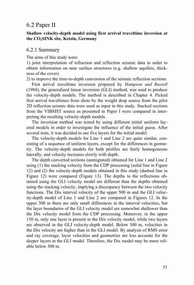
6.2 Paper II ...............................................................................................51 6.2.1 Summary.....................................................................................51 6.2.2 Conclusions ................................................................................54
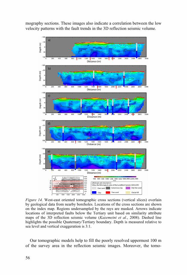
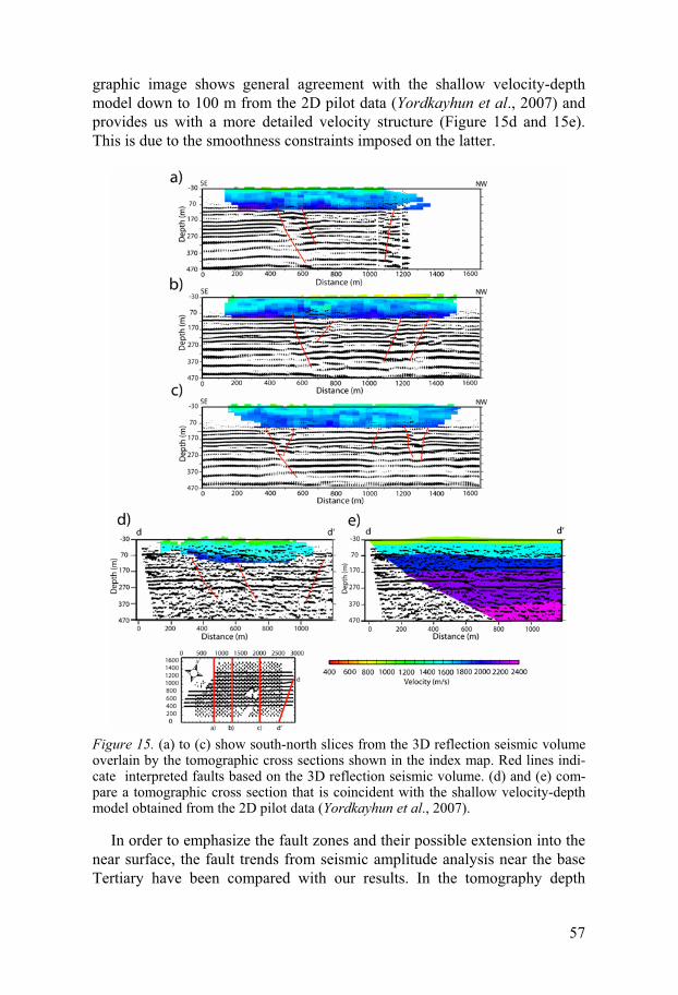
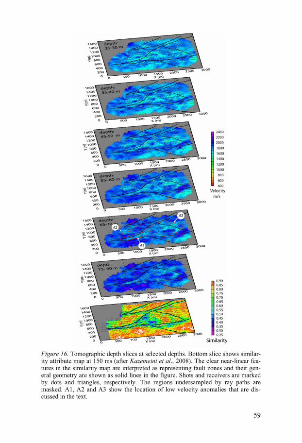
6.3 Paper III..............................................................................................54 6.3.1 Summary.....................................................................................54 6.3.2 Conclusions ................................................................................58
6.4 Paper IV..............................................................................................60 6.4.1 Summary.....................................................................................60 6.4.2 Conclusions ................................................................................66
7. Concluding remarks ..................................................................................67 7.1 General conclusions ...........................................................................67 7.2 Outlook...............................................................................................68
7.2.1 The feasibility study of fault seal and gas chimney detection ....68 7.2.2 Further improvements.................................................................70 7.2.3 Final remarks ..............................................................................71
8. Summary in Swedish ................................................................................72
1D One-dimensional 2D Two-dimensional 3D Three-dimensional 4D Four-dimensional CDP Common Depth Point CMP Common Mid Point CO2 Carbon dioxide dB Decibel DMO Dip moveout GLI Generalized Linear Inversion Hz Hertz km Kilometer m Meter ms Millisecond NMO Normal moveout RMS Root mean square S/N Signal-to-noise SVD Singular value decomposition
9
1. Introduction
The research presented in this thesis deals with 2D and 3D seismic reflection data acquired in the pre-injection stage at a CO2 geological storage site (the CO2SINK project). The thesis is split into two parts. The first part, which consists of a series of chapters, presents the summary of some theoretical aspects and research works during four years of my PhD study at Uppsala University. The second part of this thesis is a collection of papers.
The thesis begins with background information concerning the CO2 geo-logical storage and an overview of the CO2SINK project. Motivation and general objectives of the thesis are given. Then, in Chapter 2, I present sum-mary information of the geology and hydrogeology of the study area and datasets used for this thesis. Some basic concepts of seismic methods are provided in Chapter 3. A few remarks on 2D and 3D seismic imaging are also mentioned in this chapter. The two following chapters describe the methods used for my research. In Chapter 4 the basic principles underlying inverse theory are introduced, followed by a detailed description of seismic traveltime inversion techniques for constructing the velocity model in Paper II and Paper III; generalized linear inversion and tomography. Both tech-niques are refraction-based methods. Chapter 5 reviews some considerations on acquisition, processing and interpretation of seismic reflection data rele-vant to my work. The summaries of the four papers are presented in Chapter 6. I complete the thesis in Chapter 7 with a summary of the results and a discussion on problems encountered, possible improvements and outlooks. In Chapter 8, a brief summary of the thesis is given in Swedish.
The last part of the thesis is a collection of my papers, including a pub-lished paper, a manuscript in press, an accepted manuscript and a submitted manuscript. 1.1 The CO2SINK project: The challenge in the global warming problem Statistical analysis show a slight increase in global average annual tempera-tures in the last 150 years in the order of 0.76 �C (IPCC, 2007; Bachu, 2008). By prediction, mankind faces significant climate change by the end of this century as a result of continuing warming forecast to be in the range of 1.1-6.3 �C (depending on emission scenarios) (IPCC, 2007; Bachu, 2008). It is generally accepted that the main cause of the observed global warming is
10
the increase in atmospheric concentrations of greenhouse gases, such as car-bon dioxide (CO2), methane (CH4) and nitrous oxide (N2O). In particular, increasing consumption of fossil energy resources is the main factor in the increase of CO2 concentration, the most important gas responsible for the greenhouse effect. Consequently, the development of greenhouse gas mitiga-tion technologies plays an important role as a potential response to global warming. CO2 capture and storage is becoming an increasingly important concept in this respect, beside other options, such as switching to renewable solar energy sources, nuclear energy generation and energy efficiency im-provements (Gale, 2004; IPCC, 2005; Wildenborg and Lokhorst, 2005). The principle is: capture CO2 from large sources instead of releasing it into the atmosphere, transport it to a storage site, and inject it at depths of at least several hundreds of meters.
Geological media suitable for CO2 storage must have the necessary capac-ity and injectivity, as well as be able to confine the CO2 and block its lateral migration and/or vertical leakage to other strata, shallow groundwater, soils and/or atmosphere. Such geological media are oil and gas reservoirs, deep seated coal beds, caverns and mines and deep saline aquifers that are found in sedimentary basins worldwide. Storage of gases or CO2 in these media has already been applied for many years to enhance the production of oil from oil reservoir (EOR), natural gas storage and acid gas disposal.
Since CO2 storage in geological media has to be done safely and requires public acceptance, proper monitoring systems and remediation plans need to be employed for each operation. Monitoring the fate of CO2 in the subsur-face can be done using intrusive and non-intrusive technologies. Intrusive or direct methods are based on pressure measurements and sampling subsurface fluids through observation and monitoring wells for the presence of CO2 or of tracers introduced together with the injected CO2 for monitoring purposes. Non-intrusive or indirect methods are based on imaging of the subsurface using various geophysical techniques, such as time-lapse 3D seismic imag-ing and vertical seismic profiling (VSP) to detect the presence of, and track the movement of the injected CO2 plume.
Recently, a number of commercial-scale projects, e.g. the Sleipner gas field in Norway (Arts et al., 2004) and the InSalah project in Algeria have been carried out. Various pilot projects have been implemented or are al-ready planned worldwide, mostly with government support for testing and developing technologies for monitoring the fate of the injected CO2 and de-veloping monitoring techniques. Examples are CO2 injection in a deep saline aquifer at Frio in Texas, USA, at Otway in Australia, in an abandoned oil reservoir in the Weyburn field, Canada (White et al., 2004), and in the K12-B gas field in the Dutch sector of the North Sea. The existence of these op-erations indicates that there are no major technological barriers to this tech-nology.
11
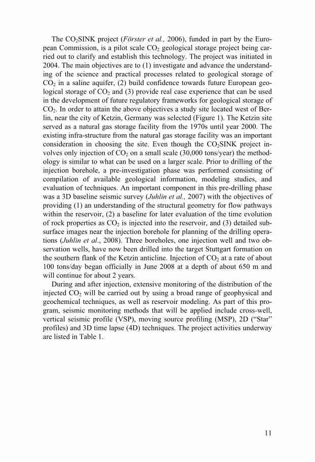
The CO2SINK project (Förster et al., 2006), funded in part by the Euro-pean Commission, is a pilot scale CO2 geological storage project being car-ried out to clarify and establish this technology. The project was initiated in 2004. The main objectives are to (1) investigate and advance the understand-ing of the science and practical processes related to geological storage of CO2 in a saline aquifer, (2) build confidence towards future European geo-logical storage of CO2 and (3) provide real case experience that can be used in the development of future regulatory frameworks for geological storage of CO2. In order to attain the above objectives a study site located west of Ber-lin, near the city of Ketzin, Germany was selected (Figure 1). The Ketzin site served as a natural gas storage facility from the 1970s until year 2000. The existing infra-structure from the natural gas storage facility was an important consideration in choosing the site. Even though the CO2SINK project in-volves only injection of CO2 on a small scale (30,000 tons/year) the method-ology is similar to what can be used on a larger scale. Prior to drilling of the injection borehole, a pre-investigation phase was performed consisting of compilation of available geological information, modeling studies, and evaluation of techniques. An important component in this pre-drilling phase was a 3D baseline seismic survey (Juhlin et al., 2007) with the objectives of providing (1) an understanding of the structural geometry for flow pathways within the reservoir, (2) a baseline for later evaluation of the time evolution of rock properties as CO2 is injected into the reservoir, and (3) detailed sub-surface images near the injection borehole for planning of the drilling opera-tions (Juhlin et al., 2008). Three boreholes, one injection well and two ob-servation wells, have now been drilled into the target Stuttgart formation on the southern flank of the Ketzin anticline. Injection of CO2 at a rate of about 100 tons/day began officially in June 2008 at a depth of about 650 m and will continue for about 2 years.
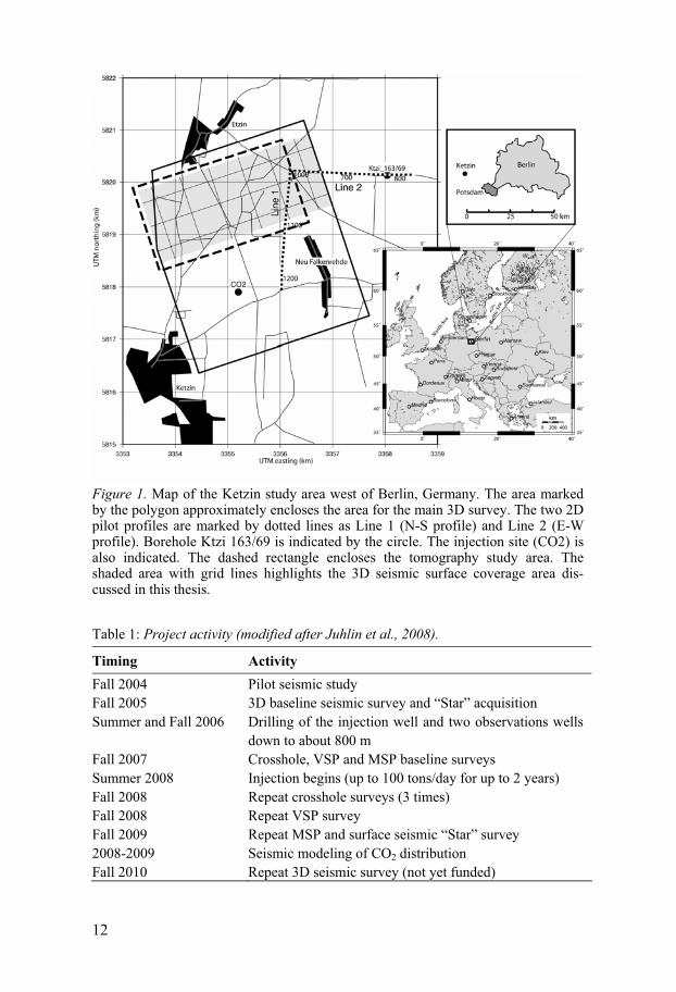
During and after injection, extensive monitoring of the distribution of the injected CO2 will be carried out by using a broad range of geophysical and geochemical techniques, as well as reservoir modeling. As part of this pro-gram, seismic monitoring methods that will be applied include cross-well, vertical seismic profile (VSP), moving source profiling (MSP), 2D (“Star” profiles) and 3D time lapse (4D) techniques. The project activities underway are listed in Table 1.
12
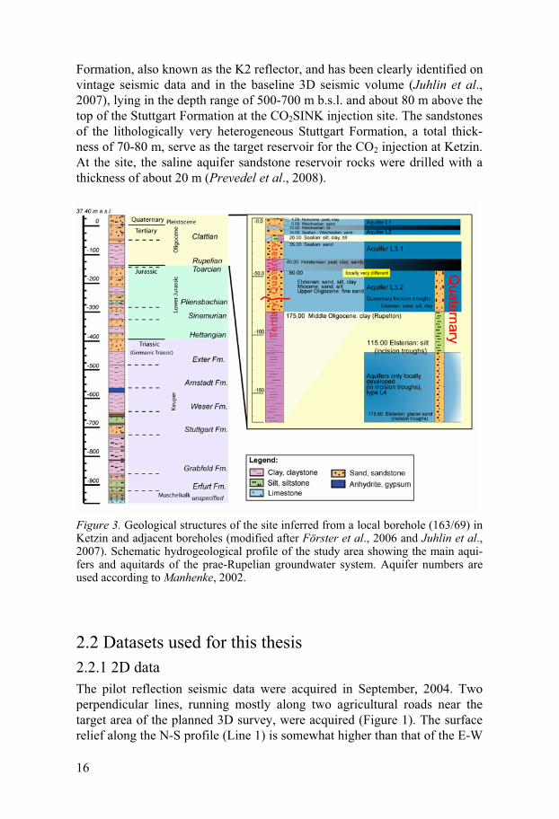
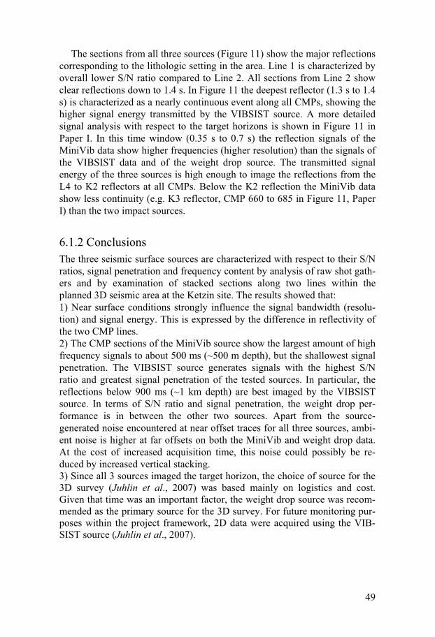
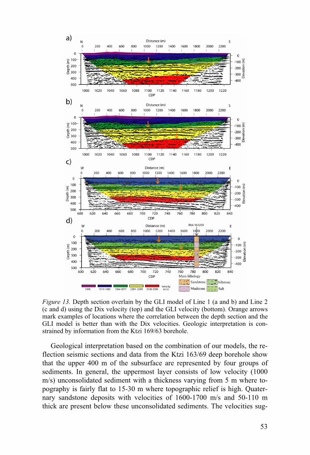
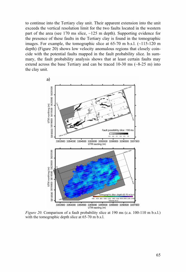
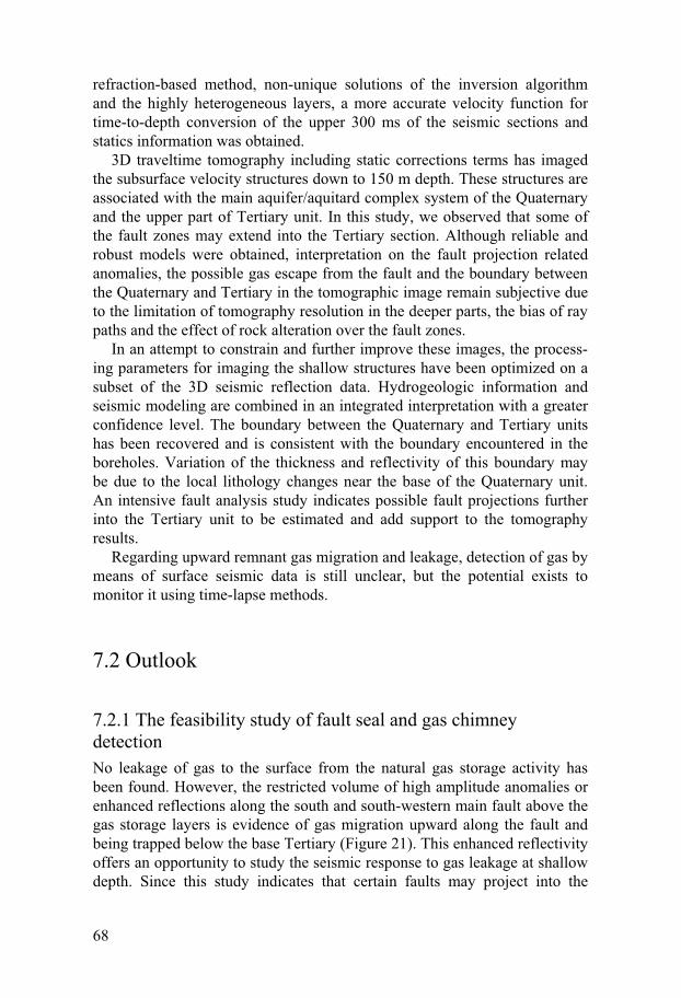
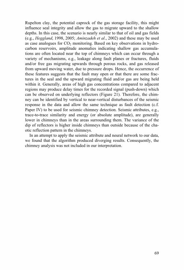
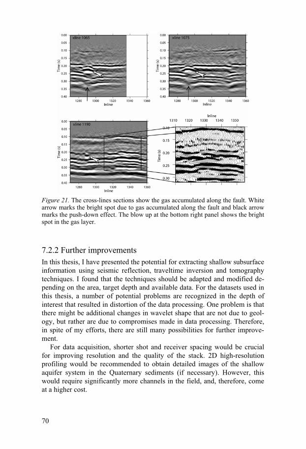
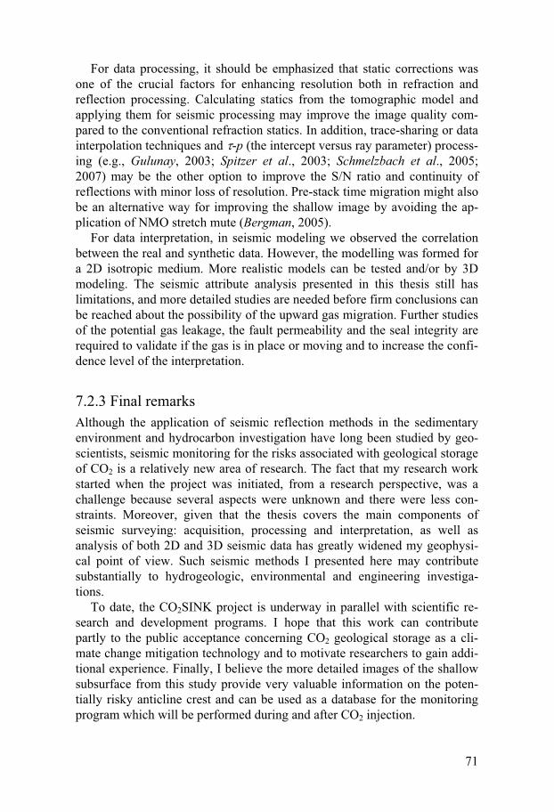
Figure 1. Map of the Ketzin study area west of Berlin, Germany. The area marked by the polygon approximately encloses the area for the main 3D survey. The two 2D pilot profiles are marked by dotted lines as Line 1 (N-S profile) and Line 2 (E-W profile). Borehole Ktzi 163/69 is indicated by the circle. The injection site (CO2) is also indicated. The dashed rectangle encloses the tomography study area. The shaded area with grid lines highlights the 3D seismic surface coverage area dis-cussed in this thesis.
Table 1: Project activity (modified after Juhlin et al., 2008).
Timing Activity Fall 2004 Fall 2005 Summer and Fall 2006 Fall 2007 Summer 2008 Fall 2008 Fall 2008 Fall 2009 2008-2009 Fall 2010
Pilot seismic study 3D baseline seismic survey and “Star” acquisition Drilling of the injection well and two observations wells down to about 800 m Crosshole, VSP and MSP baseline surveys Injection begins (up to 100 tons/day for up to 2 years) Repeat crosshole surveys (3 times) Repeat VSP survey Repeat MSP and surface seismic “Star” survey Seismic modeling of CO2 distribution Repeat 3D seismic survey (not yet funded)
13
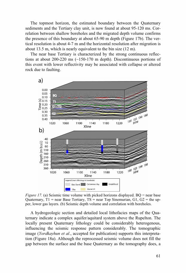
1.2 Motivation and research objectives As mentioned in the previous section, the focus of seismic investigations at the CO2SINK project is on site characterization and monitoring of the upper 1 km of the sedimentary environment. The scope of this thesis covers two components: to compare the seismic sources in conjunction with optimizing 3D surveys, and to study the potential of imaging the shallow subsurface by means of high resolution seismic techniques. Figure 1 shows the location of the data sets discussed in the thesis. The main focus has been to study in detail the crest of the anticline. However, 2D seismic lines further east were initially studied.
A pilot 2D seismic reflection survey was acquired as a preparatory work before carrying out the 3D baseline seismic survey at the Ketzin site. One of the main goals of this study was to test different acquisition parameters, so that the results could be used to guide the planning of the 3D survey. Since the 3D seismic survey would require a large number of source points, several factors with respect to the seismic source needed to be considered. There-fore, in my first study (Paper I) I focused on the comparison of the three seismic sources tested in this pilot study. From this point, the results were used as input to optimize the 3D seismic survey. Acquisition and processing schemes for this 3D seismic study have been discussed in detail by Juhlin et al. (2007), which included the full 3D volume, and a presentation of the seismic images and their associated geologic interpretation.
Results of the 2D and 3D seismic processing show that the deeper part of the subsurface was clearly imaged, but some details were lost in the upper-most part due to resolution limits, acquisition geometry and processing arte-facts. Consequently, my following studies (Paper II, III and IV) I focused on the application of high resolution seismic techniques by integrating seismic reflection and seismic refraction methods to study the potential for improv-ing the image of the upper 400 m. This depth range hosts caprock, shallow faults, an aquifer system, and the abandoned natural gas storage formations. Thus, characterizing the shallow subsurface is important in terms of initial site delineation of potential leakage paths and monitoring and risk assess-ment after CO2 has been injected. Due to the complicated nature of the near surface environment, high resolution is required to obtain detailed images. However, for the depth of interest, interference between source-generated noise and shallow reflections, near surface effects and time shifts, are all the challenges. Especially, these time shifts are comparable to the dominant periods of the reflections and to the size of the target structures. This limit to what degree the shallow structures may be imaged. Therefore, the main ef-fort is to optimize the application of high resolution seismic techniques and reconstruct the near surface model with greater accuracy and higher resolu-tion in order to fill the gap between the deep and shallow parts of the subsur-face.
14
2. Overview of site geology, hydrogeology and seismic data
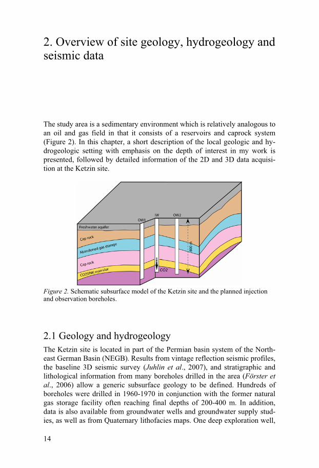
The study area is a sedimentary environment which is relatively analogous to an oil and gas field in that it consists of a reservoirs and caprock system (Figure 2). In this chapter, a short description of the local geologic and hy-drogeologic setting with emphasis on the depth of interest in my work is presented, followed by detailed information of the 2D and 3D data acquisi-tion at the Ketzin site.
Figure 2. Schematic subsurface model of the Ketzin site and the planned injection and observation boreholes.
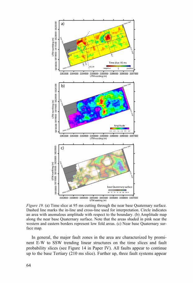
2.1 Geology and hydrogeology The Ketzin site is located in part of the Permian basin system of the North-east German Basin (NEGB). Results from vintage reflection seismic profiles, the baseline 3D seismic survey (Juhlin et al., 2007), and stratigraphic and lithological information from many boreholes drilled in the area (Förster et al., 2006) allow a generic subsurface geology to be defined. Hundreds of boreholes were drilled in 1960-1970 in conjunction with the former natural gas storage facility often reaching final depths of 200-400 m. In addition, data is also available from groundwater wells and groundwater supply stud-ies, as well as from Quaternary lithofacies maps. One deep exploration well,
15
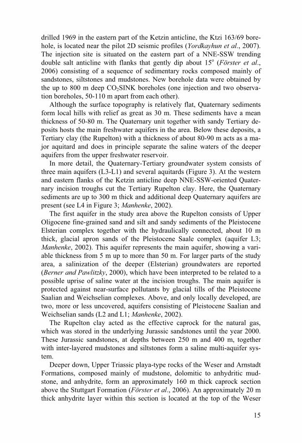
drilled 1969 in the eastern part of the Ketzin anticline, the Ktzi 163/69 bore-hole, is located near the pilot 2D seismic profiles (Yordkayhun et al., 2007). The injection site is situated on the eastern part of a NNE-SSW trending double salt anticline with flanks that gently dip about 15o (Förster et al., 2006) consisting of a sequence of sedimentary rocks composed mainly of sandstones, siltstones and mudstones. New borehole data were obtained by the up to 800 m deep CO2SINK boreholes (one injection and two observa-tion boreholes, 50-110 m apart from each other).
Although the surface topography is relatively flat, Quaternary sediments form local hills with relief as great as 30 m. These sediments have a mean thickness of 50-80 m. The Quaternary unit together with sandy Tertiary de-posits hosts the main freshwater aquifers in the area. Below these deposits, a Tertiary clay (the Rupelton) with a thickness of about 80-90 m acts as a ma-jor aquitard and does in principle separate the saline waters of the deeper aquifers from the upper freshwater reservoir.
In more detail, the Quaternary-Tertiary groundwater system consists of three main aquifers (L3-L1) and several aquitards (Figure 3). At the western and eastern flanks of the Ketzin anticline deep NNE-SSW-oriented Quater-nary incision troughs cut the Tertiary Rupelton clay. Here, the Quaternary sediments are up to 300 m thick and additional deep Quaternary aquifers are present (see L4 in Figure 3; Manhenke, 2002).
The first aquifer in the study area above the Rupelton consists of Upper Oligocene fine-grained sand and silt and sandy sediments of the Pleistocene Elsterian complex together with the hydraulically connected, about 10 m thick, glacial apron sands of the Pleistocene Saale complex (aquifer L3; Manhenke, 2002). This aquifer represents the main aquifer, showing a vari-able thickness from 5 m up to more than 50 m. For larger parts of the study area, a salinization of the deeper (Elsterian) groundwaters are reported (Berner and Pawlitzky, 2000), which have been interpreted to be related to a possible uprise of saline water at the incision troughs. The main aquifer is protected against near-surface pollutants by glacial tills of the Pleistocene Saalian and Weichselian complexes. Above, and only locally developed, are two, more or less uncovered, aquifers consisting of Pleistocene Saalian and Weichselian sands (L2 and L1; Manhenke, 2002).
The Rupelton clay acted as the effective caprock for the natural gas, which was stored in the underlying Jurassic sandstones until the year 2000. These Jurassic sandstones, at depths between 250 m and 400 m, together with inter-layered mudstones and siltstones form a saline multi-aquifer sys-tem.
Deeper down, Upper Triassic playa-type rocks of the Weser and Arnstadt Formations, composed mainly of mudstone, dolomitic to anhydritic mud-stone, and anhydrite, form an approximately 160 m thick caprock section above the Stuttgart Formation (Förster et al., 2006). An approximately 20 m thick anhydrite layer within this section is located at the top of the Weser
16
Formation, also known as the K2 reflector, and has been clearly identified on vintage seismic data and in the baseline 3D seismic volume (Juhlin et al., 2007), lying in the depth range of 500-700 m b.s.l. and about 80 m above the top of the Stuttgart Formation at the CO2SINK injection site. The sandstones of the lithologically very heterogeneous Stuttgart Formation, a total thick-ness of 70-80 m, serve as the target reservoir for the CO2 injection at Ketzin. At the site, the saline aquifer sandstone reservoir rocks were drilled with a thickness of about 20 m (Prevedel et al., 2008).
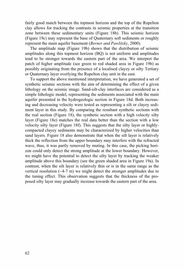
Figure 3. Geological structures of the site inferred from a local borehole (163/69) in Ketzin and adjacent boreholes (modified after Förster et al., 2006 and Juhlin et al., 2007). Schematic hydrogeological profile of the study area showing the main aqui-fers and aquitards of the prae-Rupelian groundwater system. Aquifer numbers are used according to Manhenke, 2002.
2.2 Datasets used for this thesis 2.2.1 2D data The pilot reflection seismic data were acquired in September, 2004. Two perpendicular lines, running mostly along two agricultural roads near the target area of the planned 3D survey, were acquired (Figure 1). The surface relief along the N-S profile (Line 1) is somewhat higher than that of the E-W
17
profile (Line 2). Surface conditions along the two lines varied. Line 1 was a traditional agricultural road, while Line 2 consisted of a hard soil that had been compressed by heavy military equipment. The pilot study consisted of testing both source and receiver performance. Three different sources were tested along the two lines (Table 2). The meas-urements were carried out according to the same scheme for every source. On the first day, tests and parameter tuning were done at five selected loca-tions on or close to Line 2. On the following 2-3 days, data were acquired by shooting at all stations (source and receiver spacing of 20 m) on both pro-files, allowing CMP stacked sections to be produced. Data were recorded on 240 channels (fixed spread). Sources activated on Line 1 were also recorded on Line 2, and vice versa, providing the possibility for a (pseudo) 3D analy-sis of the survey area. Only a few selected source stations were skipped due to the presence of underground gas lines. The tests also included comparison of 10 Hz and 28 Hz single geophones and 10 Hz geophone arrays on Line 2 and a comparison of geophones planted on the surface and in holes 30-40 cm deep. A summary of the acquisition parameters is provided in Table 2.
Table 2: Acquisition parameters of 2D seismic data. Parameter Detail Sources Weight drop, VIBSIST and MiniVib Profile Length Number of stations/line Number of shots/line Shots per station
2.4 km 120 stations 113-115 (Weight drop), 107-114 (VIBSIST) and 71-117 (MiniVib) 5-8 (Weight drop), 3 (VIBSIST) and 5 (MiniVib)
Receivers Natural geophone frequency Spacing
10 Hz and 28 Hz (single) 20 m
Recording Recording system Record length Sweep length Sampling interval
SERCEL 408 system 3 s (Weight drop), 30 s (VIBSIST) and 18.5 s (MiniVib) 27 s (VIBSIST) and 16 s (MiniVib) 1 ms
2.2.2 3D data A 3D baseline seismic survey covering about 12 km2 was acquired in the autumn of 2005. The acquisition parameters are shown in Table 3. The seis-mic survey was carried out using a template scheme. Each template had the
18
same internal geometry, consisting of 240 recording stations and 200 nomi-nal source points. The receivers were deployed along 5 lines 96 m apart, lying perpendicular to 12 source lines 48 m apart. Receiver station spacing and source station spacing was 24 m, and every 6th source station was skipped in order to optimize the acquisition with a resulting nominal fold of 25 for 12 x 12 m CDP bins. The templates were deployed in an overlapping scheme to reduce the acquisition footprint. Because of logistical difficulties, all of the source and receiver stations were not available at all stations, re-sulting in reduced coverage in some areas. An accelerated weight drop source was used and repeated shots at the same position were stacked in order to enhance the signal. The receivers were placed at about 20-30 cm depth, and the data were recorded using a 1 ms sampling rate with a 3 s re-cord length.
Table 3: Acquisition parameters of 3D seismic data. Parameter Detail Sources Shots per source point Spacing
Weight drop 8-9 24 m
Receivers Natural geophone frequency Spacing / channels
28 Hz (single) 24 m / 48
Template Source line spacing/number Receiver line spacing/number CDP bin size Nominal fold
48 m / 12 96 m / 5 12 m x 12 m 25
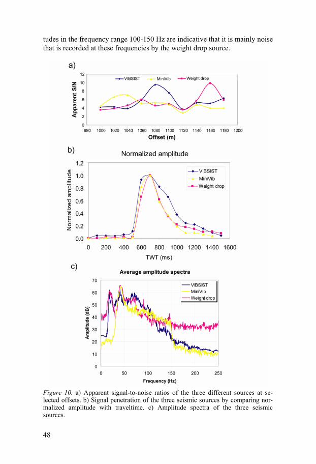
Recording Recording system Record length Sampling interval
SERCEL 408 system 3 s 1 ms
19
3. Basic concepts of seismic methods
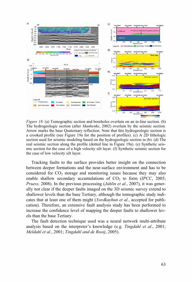
Seismic investigations of the earth involve observing waves after they have passed through the media and then reconstructing details of the media from the details of the observed wave field. Two types of waves are essentially used: reflected and refracted. In this chapter, some basic concepts of seismic methods which are relevant to my work are briefly reviewed. The theoretical background is mainly adapted and summarized from a number of publica-tions (e.g., Yilmaz, 1987; Sheriff and Geldart, 1995; Brouwer and Helbig, 1998; Biondi, 2007).
3.1 The wave equation The seismic method utilizes the propagation of waves through the earth. The propagation of seismic waves is described by the wave equation. This wave equation arises from the fundamental physics of the problem under the as-sumption of small particle displacements which can be derived from the relation between tension, elasticity, Hooke’s law and Newton’s second law of motion (Yilmaz, 1987; Sheriff and Geldart, 1995; Aki and Richards, 2002). The nature of wave propagation can be very complex, and the various methods use simplifications of various types in order to make the problem tractable. For wave propagation in homogeneous, isotropic, and elastic me-dia, the wave equation can be written in the form of the equation of motion for the displacement vector u = (u, v, w):
uu 22
2
)( �������� ��
t (1)
where and � are known as the Lamé elastic properties, and is density.
zyx ��
���
���
�� kji , zw
yv
xu
��
���
���
�� , and the Laplacian operator,
2
2
2
2
2
22
zyx ��
���
���
�� .
20
The wave equation can be expressed in vector as well as the more con-ventional scalar notation. For a homogeneous isotropic medium, the scalar wave equation can be written in the general form:
������ 22
2
2
1tV
(2)
where V is a constant. The quantity � is inferred to be some disturbance (particles motion) that is propagated from one point to another with speed V. This disturbance is commonly referred to as a P-wave (or compressional, longitudinal wave) when the motion is in the direction of wave propagation and an S-wave (or transverse, shear, rotational wave) when the motion is in the direction perpendicular to the direction of wave propagation. Equation 1 can be specialized to describe various wave types that travel within solids and fluids (body wave), and along free surfaces and layer boundaries (sur-face waves). Body waves (P- and S- waves) are important in exploration seismology whereas surface waves are generally of more interest in earth-quake seismology. The wave equation is mainly used for modeling and in-version of seismic waves. In general, it is sufficient to consider the wave equation in geometrical terms, i.e., wavefronts or rays as in optics, because when the wavelength is small compared to other geometrical features, wave behaves as if it travels along rays (Born and Wolf, 1964).
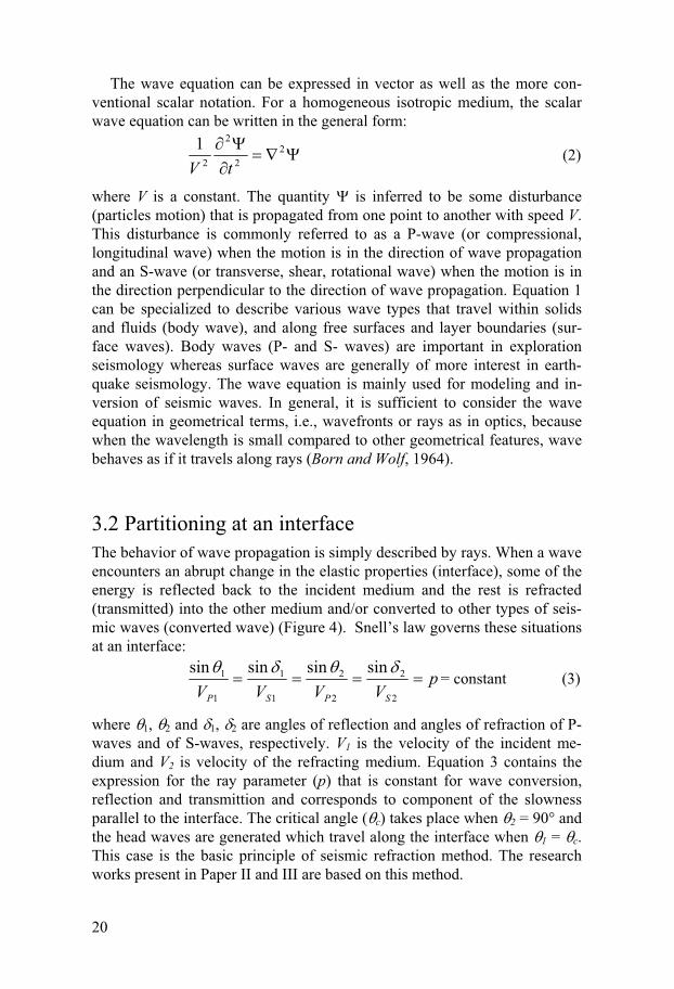
3.2 Partitioning at an interface The behavior of wave propagation is simply described by rays. When a wave encounters an abrupt change in the elastic properties (interface), some of the energy is reflected back to the incident medium and the rest is refracted (transmitted) into the other medium and/or converted to other types of seis-mic waves (converted wave) (Figure 4). Snell’s law governs these situations at an interface:
pVVVV SPSP
����2
2
2
2
1
1
1
1 sinsinsinsin � � = constant (3)
where 1, 2 and �1, �2 are angles of reflection and angles of refraction of P-waves and of S-waves, respectively. V1 is the velocity of the incident me-dium and V2 is velocity of the refracting medium. Equation 3 contains the expression for the ray parameter (p) that is constant for wave conversion, reflection and transmittion and corresponds to component of the slowness parallel to the interface. The critical angle ( c) takes place when 2 = 90� and the head waves are generated which travel along the interface when 1 = c. This case is the basic principle of seismic refraction method. The research works present in Paper II and III are based on this method.
21
Boundary conditions allow calculations of how wave energy is divided among reflected and transmitted waves. At the interface, stress field and displacements field must be continuous. The simple approach in terms of displacements yields Zoeppritz’ equations, which states that the reflection amplitude compared with the incident amplitude varies directly as the change in acoustic impedance (Sheriff and Geldart, 1995). Where acoustic impedance (Z) is given by:
Z=VP (4)
Generally speaking from equation 4, the harder the rock the greater its acoustic impedance.
Figure 4. Partitioning at an interface showing refracted wave, reflected wave and converted wave.
At normal incidence ( 1 = 0�), which is normally assumed in most reflec-tion work, Zoeppritz’ equations can be written for the normal reflection co-efficient (R) and transmission (T) coefficients following the simple forms:
1122
11
12
1
1122
1122
12
12
22||1PP
P
PP
PP
VVV
ZZZRT
VVVV
ZZZZR
��
����
��
���
�
(5)
where Z1 and Z2 is the acoustic impedance in the incident medium and in the refraction medium, respectively. A negative value of R indicates a 180o phase change in the reflected ray. It is generally accepted that the normal incidence formulas can be used for slight deviation from the normal ( 1 � 15�) without introducing considerable error.
At non-normal incidence ( 1 � 0�), the reflection and refraction coeffi-cients are very algebraically complicated functions of the P- and S-wave
22
velocities and densities in the two media as well as the angles of reflection and refraction of the P- and S-waves. Reflection at non-normal incidence leads to wave conversion and amplitude changes, especially near the critical angle (Sheriff and Geldart, 1995).
3.3 Seismic velocity Understanding and interpreting seismic velocity is important for conversion from traveltime to depth, modeling, imaging of the data (migration), classifi-cation and filtering of signal and noise, predictions of the lithology and aid-ing geological interpretation (Brouwer and Helbig, 1998). According to equation 1 and 2, the P-wave velocity (Vp) and S-wave velocity (Vs) is ex-pressed by:
��
� 3
42 ��
��PV (6)
�
�SV (7)
where � is the bulk modulus and is density. � is also called shear modulus. In fluids, � =0, i.e., there are no shear waves. The P-wave velocity is always greater than the S-wave velocity.
Although equations 6 and 7 imply that velocity increases as density de-creases, the seismic velocity in actual rocks depends on many factors, in-cluding lithology, porosity, degree of compaction, pore filling interstitial fluid, temperature and pressure, etc. (Brouwer and Helbig, 1998; Wang, 2001). This means that the elastic properties vary as well. In general, density increases with increasing velocity and the velocity-density relationship for porous rocks (e.g., sediments, near seafloor basalts) can be estimated by the Gardner relation (Gardner et al., 1974):
4/1aV� (8)
where a=310 in SI units. Although the velocity of P-wave propagation is a fundamental physical property of rocks (Amery, 1993), velocity alone does not provide a good basis for distinguishing lithology because velocity ranges are so broad and there is so much overlaps (see Table 4). Measurements of velocities can be done by laboratory measurements using probes, borehole measurements, refraction seismics, analysis of reflection hyperbolas and vertical seismic profiling, etc.
23
Table 4: Examples for typical velocities of rocks (after Kearey and Brooks, 1991).
Material P-wave velocity, Vp (km/s) Unconsolidated Material Sand (dry) Sand (water saturated) Clay Glacial till (water saturated) Permafrost
1.3-1.4 Other materials Steel Iron Aluminium Concrete
6.1 5.8 6.6 3.6
3.4 Seismic resolution The resolution of seismic data is given by the ability to separate two features that are very close together (Sheriff, 1991). Resolution can be considered in both the vertical and lateral directions and is referred to as vertical and lat-eral resolution (also called horizontal resolution), respectively. Both are gen-erally controlled by spectral bandwidth.
Vertical resolution tells us how far apart two interfaces must be to show up as separate reflectors. The shape of the seismic pulse (seismic wavelet)
24
determines the vertical resolution of the seismic method. The acceptable threshold for vertical resolution is about one quarter of the dominant wave-length (�/4, the Rayleigh criterion). The dominant wave length of seismic waves is =v/f, where v is velocity and f is the dominant frequency. The common situation encountered in reservoir geophysics where a thin bed, e.g., a wedge or pinch out feature exists is the tuning effect. When a bed embedded in a medium of different properties is ¼ wavelength in thickness, the reflection from the top and base of the bed interfere constructively and the amplitude increases. This situation was observed in the Ketzin data as well.
Lateral resolution reveals how close two reflecting points can be situated horizontally, yet be recognized as two separate points rather than one (Yil-maz, 1987). The lateral resolution is given by the size of the first Fresnel zone (Figure 5a). The Fresnel zone is defined as the subsurface area, which reflects energy that arrives at the earth’s surface within a time delay equal to half the dominant period (T/2). In this case ray paths of reflected waves dif-fer by less than half a wavelength. A commonly accepted value is one-fourth the signal wavelength. A recorded reflection at the surface is not coming from a subsurface point, but from a disk shaped area, which has a dimension equal to the Fresnel zone (Yilmaz, 1987; Sheriff and Geldart, 1995). The radius of the Fresnel zone (r) is given by:
ftvz
r 00
22��
(9)
where z0 is the depth of the reflecting interface and t0=2z0/v is the two-way traveltime and f is the dominant frequency. This equation shows that high frequencies give better resolution than low frequencies and resolution dete-riorates with depth and with increasing velocities. The shape and size of the Fresnel zone also depend on the position of source and receiver, the velocity distribution, wave length, and on depth, dip, and curvature of the reflector (Brouwer and Helbig, 1998).
Improvement of seismic resolution comes initially from improvement of frequency bandwidth of the data (shaping the spectrum). The migration process is the final step to bring lateral and vertical resolution in accordance. 3D migration is a major factor that drastically improves 3D imaging com-pared with 2D data as the energy is far better focused (Spitzer et al., 2003; Schmelzbach et al., 2007). Migration can be considered as a downward con-tinuation of receivers from the surface to the reflector making the Fresnel zone smaller and smaller. The process will shorten the radius of the Fresnel zone in all directions (Figure 5b), improving drastically the lateral resolu-tion.
25
Figure 5. a) 2D view illustrating the first Fresnel zone. b) Top view illustrating Fresnel zone before and after 2D and 3D migration (after Chaouch and Mari, 2006).
3.5 2D versus 3D seismic surveys 2D seismic reflection techniques have proven to be a useful tool for imaging subsurface structures in a variety of scales and investigations (e.g., Steeplesand Miller, 1990; Francese et al., 2002; Juhlin et al., 2002; Hammer et al., 2004). 3D seismic reflection techniques have been used widely in hydrocar-bon exploration. Descriptions of shallow 3D seismic reflection surveys on land started to appear in the late 1990s (Buker et al., 1998). Recently, there is a trend of substantial reduction in costs related to acquisition and process-ing of 3D data (Buker et al., 2000; Spitzer et al., 2001; 2003) resulting in small-scale 3D surveys becoming even more common. 2D seismic data are normally used to obtain a regional overview in an area because such data are relatively cheap to acquire, compared to 3D seismic data. However, for more detailed mapping, 3D seismic data are required. The benefits of 3D seismic over conventional 2D seismic includes; 3D images usually contain less source-generated noise (Sheriff and Geldart, 1995), and a dramatic increase in information and accuracy of structural images of the subsurface.
For 2D acquisition, we assume implicitly that the earth is a cylinder, the axis of which is orthogonal to the direction of the survey. However, this assumption is not fulfilled. Thus, interpretation of 2D seismic produces a distorted image. Following Biondi (2007) Figure 6 shows the main reasons why 2D seismic interpretation produces distorted images when one is imag-ing 3D structures. The point diffractor R3d is out-of-the-plane with respect to the 2D acquisition direction. Reflections are incorrectly back-propagated in the earth along the vertical plane passing through the acquisition direction, and are imaged at the wrong location, R2d. To image the diffractor at its cor-rect location, R3d, one must apply 3D imaging for back-propagating the re-corded reflection along an oblique plane. However, even after applying 3D imaging methods to a single 2D line, one would be left with the ambiguity of
26
where to place the diffractor along the semicircular curve perpendicular to the acquisition direction, marked as “crossline migration” in Figure 6. To resolve this ambiguity, one estimates the crossline component of the propa-gation direction, that is, by recording 3D data.
For 2D imaging, the error in positioning of the diffractor has both a crossline direction component, �y and a depth component, �z. The reflector R2d should be moved along a semicircle in the crossline direction to be placed at its correct position, R3d. Where the velocity is constant, this semi-circular trajectory corresponds to the semicircle of a zero-offset crossline migration. The analytical expression of this semicircle is independent of velocity and depends only on the apparent depth d of the reflector; that is �y2
+ (d-�z)2 = d2. Therefore, in this simple case the imaging of 3D data can be performed as two steps: (1) imaging along 2D lines, followed by (2) crossline migration. However, where the propagation velocity is not con-stant, this simple decomposition of 3D imaging is not correct, and full 3D migration is required.
Figure 6. Imaging of an out-of-plane diffractor (modified after Biondi, 2007). In 2D acquisition and imaging, only the in-plane propagation direction can be determined. In 3D acquisition and processing, data contained in the red traces allow unambigu-ous determination of the propagation direction and position of the diffractor.
27
Extra information 3D seismic information not only can increase the accuracy of structural im-ages of the subsurface, but can also provide a wealth of stratigraphic infor-mation that is not present in 2D seismic data. Horizontal slicing of 3D data volumes facilitates structural interpretations by allowing critical horizons and other features (e.g., faults, channels) to be identified and mapped. Re-cording data with a wide source-receiver azimuth provides additional infor-mation of subsurface targets. This additional illumination may be crucial to generation of interpretable images where targets lie under complex overbur-den. The availability of high-resolution 3D images has also paved the way for time-lapse seismic data, which is referred to as 4D seismic data.
New challenges Many of the basic concepts developed for 2D seismic imaging are still valid for 3D imaging. However, 3D imaging presents several new problems that are caused by the higher dimensionality of 3D data, leading to large amounts of data being recorded in the field. Such large quantities are difficult to han-dle, visualize, and process. An important aspect of processing a large 3D data set is to devise the right strategy for reducing the time and resources necessary for obtaining an image of the subsurface, without compromising the accuracy of the results.
28
4. First arrival traveltime inversion and tomography
This chapter provides details on the specialized processing methods I applied to the 2D and 3D seismic data. Traveltime inversion and tomography for solving for the near-surface velocity structure was performed on first arrival time picks from the datasets. The first arrivals are assumed to be the onset of head waves refracted at the refracting interfaces and diving waves. To better understand the techniques, the basic principle of traveltime inversion is in-troduced.
4.1 Introduction to inverse theory Inverse theory provides a mathematical framework to construct a suitable image (model) of some physical quantity based on a set of measured data (Tarantola, 1987; Menke, 1989; Parker, 1994). To find the best earth model when observation data are given is called an inverse problem. On the other hand, to determine what kind of signal a given geophysical model would give is referred to as a forward problem. A general form of the relationship between data and model parameters can be written as a system of equations:
Gm = d (10) where d is the vector of the observations, G is the kernel matrix that relates the model to the observation, and m is the vector containing model parame-ters. The kernel function represents the physics of the problem, including boundary conditions and differential equations.
The inversion process involves computing the inverse of matrix G and then multiplying this matrix by the data d to compute the model m. How-ever, this inverse matrix can be difficult to compute, particularly if the ma-trix is ill-conditioned (small data errors cause large model changes), ill posed (mixed-determined), or large (too many parameters for the available com-puter memory).
Many of the inverse problems in geophysics are nonlinear and do not have a unique solution. Therefore, a direct inverse solution cannot be found using the traditional mathematical approach. For nonlinear problems we usually linearize the equations and iterate.
29
A least squares approach is often used to find a solution (Menke, 1989). However, the inverse solution will generally be unstable and the problem must be constrained or regularized in some way. We must add information, apriori information, or some measure of the length of the solution. Then we determine a solution that minimizes some combination of prediction error (E) and solution length (L):
�(m) = E+�2L (11) where � is a trade-off parameter. In these cases, a weighted damped least squares approach gives the solution (Menke, 1989; Clement and Knoll, 2006):
mest = <m>+[GTWeG + �2Wm]-1 GTWe[d-G<m>] (12) where mest is the best fitting model, <m> is the starting model, d and G are the data and the kernel as before, Wm is the regularization or model weight-ing matrix, and We is the data weighting matrix. The parameter � determines how much the data influences the model versus how much the model is con-strained by the regularization. For � = 0, the solution depends only on the data. For large values, the solution depends more on the regularization. A variety of computational methods have been developed to implement matrix inversions, such as, ART (e. g., Peterson et al., 1985), SIRT (e. g., Trampert and Levequ,1990) and conjugate gradient methods, e.g., LSQR (Paige and Saunders, 1982), which are all iterative solvers.
It is often easy to obtain an image from an inversion algorithm, but the challenge is to obtain the “best” image possible so that the data contributes maximally toward the solution of the particular problem. Quality interpreta-tions require that the interpreter understand the fundamentals regarding the non-uniqueness of the solution, how apriori information and the constraints are used to regularize the problem, and to what degree the data can be fit (Aster et al., 2005).
4.2 Generalized Linear Inversion (GLI) The Generalized Linear Inversion (GLI) approach is a powerful mathemati-cal technique that can be applied to any geophysical problem. In Paper II, the first arrival traveltime inversion technique proposed by Hampson and Rus-sell (1984) was used. It is based on ray tracing through a best-guess initial velocity model and solving the problem of optimizing the fit of the calcu-lated to observed traveltimes in a least-squares sense (Lines and Treitel, 1984; Menke, 1984). The model update procedure for either depth or veloc-ity consists of a looping process that is similar to that used in tomographic inversion as the schematic diagram in Figure 7 shows. The method is briefly outlined as follows:
30
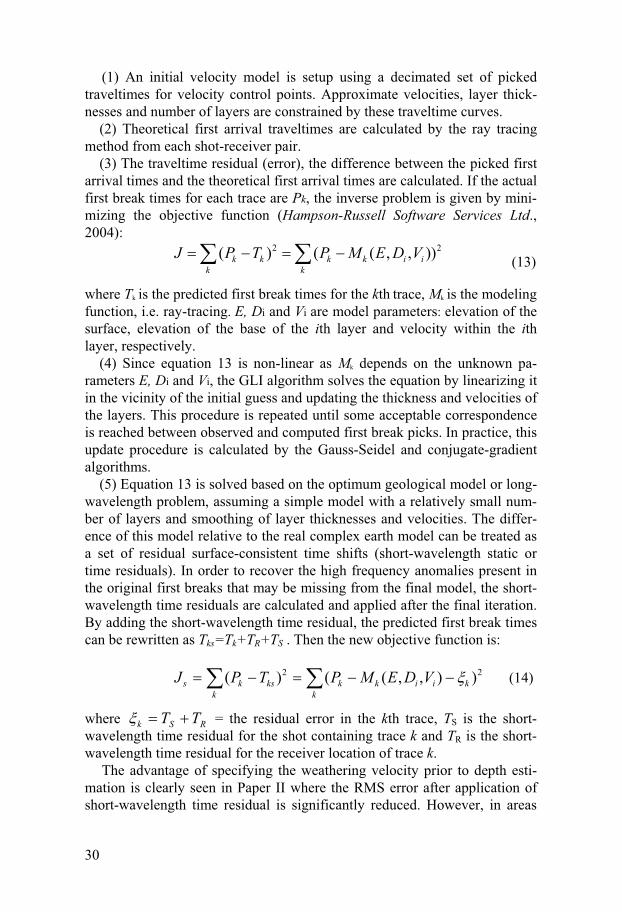
(1) An initial velocity model is setup using a decimated set of picked traveltimes for velocity control points. Approximate velocities, layer thick-nesses and number of layers are constrained by these traveltime curves. (2) Theoretical first arrival traveltimes are calculated by the ray tracing method from each shot-receiver pair. (3) The traveltime residual (error), the difference between the picked first arrival times and the theoretical first arrival times are calculated. If the actual first break times for each trace are Pk, the inverse problem is given by mini-mizing the objective function (Hampson-Russell Software Services Ltd., 2004):
2 2( ) ( ( , , ))k k k k i ik k
J P T P M E D V� � � �� � (13)
where Tk is the predicted first break times for the kth trace, Mk is the modeling function, i.e. ray-tracing. E, Di and Vi are model parameters: elevation of the surface, elevation of the base of the ith layer and velocity within the ith layer, respectively. (4) Since equation 13 is non-linear as Mk depends on the unknown pa-rameters E, Di and Vi, the GLI algorithm solves the equation by linearizing it in the vicinity of the initial guess and updating the thickness and velocities of the layers. This procedure is repeated until some acceptable correspondence is reached between observed and computed first break picks. In practice, this update procedure is calculated by the Gauss-Seidel and conjugate-gradient algorithms. (5) Equation 13 is solved based on the optimum geological model or long-wavelength problem, assuming a simple model with a relatively small num-ber of layers and smoothing of layer thicknesses and velocities. The differ-ence of this model relative to the real complex earth model can be treated as a set of residual surface-consistent time shifts (short-wavelength static or time residuals). In order to recover the high frequency anomalies present in the original first breaks that may be missing from the final model, the short-wavelength time residuals are calculated and applied after the final iteration. By adding the short-wavelength time residual, the predicted first break times can be rewritten as Tks=Tk+TR+TS . Then the new objective function is:
22 )),,(()( ki
kikkks
kks VDEMPTPJ ������ �� (14)
where RSk TT ��� = the residual error in the kth trace, TS is the short-wavelength time residual for the shot containing trace k and TR is the short-wavelength time residual for the receiver location of trace k.
The advantage of specifying the weathering velocity prior to depth esti-mation is clearly seen in Paper II where the RMS error after application of short-wavelength time residual is significantly reduced. However, in areas
31
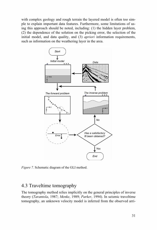
with complex geology and rough terrain the layered model is often too sim-ple to explain important data features. Furthermore, some limitations of us-ing this approach should be noted, including: (1) the hidden layer problem, (2) the dependence of the solution on the picking error, the selection of the initial model, and data quality, and (3) apriori information requirements, such as information on the weathering layer in the area.
Figure 7. Schematic diagram of the GLI method.
4.3 Traveltime tomography The tomography method relies implicitly on the general principles of inverse theory (Tarantola, 1987; Menke, 1989; Parker, 1994). In seismic traveltime tomography, an unknown velocity model is inferred from the observed arri-
32
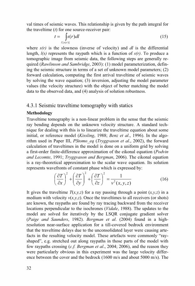
val times of seismic waves. This relationship is given by the path integral for the traveltime (t) for one source-receiver pair:
��)}({
)(rsl
dlrst (15)
where s(r) is the slowness (inverse of velocity) and dl is the differential length, l(s) represents the raypath which is a function of s(r). To produce a tomographic image from seismic data, the following steps are generally re-quired (Rawlinson and Sambridge, 2003): (1) model parameterization, defin-ing the seismic structure in terms of a set of unknown model parameters; (2) forward calculation, computing the first arrival traveltime of seismic waves by solving the wave equation; (3) inversion, adjusting the model parameter values (the velocity structure) with the object of better matching the model data to the observed data, and (4) analysis of solution robustness.
4.3.1 Seismic traveltime tomography with statics Methodology Traveltime tomography is a non-linear problem in the sense that the seismic ray bending depends on the unknown velocity structure. A standard tech-nique for dealing with this is to linearize the traveltime equation about some initial, or reference model (Kissling, 1988; Benz et al., 1996). In the algo-rithm used in Paper III, PStomo_eq (Tryggvason et al., 2002), the forward calculation of traveltimes in the model is done on a uniform grid by solving a first-order finite-difference approximation of the eikonal equation (Podvin and Lecomte, 1991; Tryggvason and Bergman, 2006). The eikonal equation is a ray-theoretical approximation to the scalar wave equation. Its solution represents wavefronts of constant phase which is expressed by:
),,(1
2
222
zyxvzT
yT
xT
����
�����
����
����
���
����
�����
(16)
It gives the traveltime T(x,y,z) for a ray passing through a point (x,y,z) in a medium with velocity v(x,y,z). Once the traveltimes to all receivers (or shots) are known, the raypaths are found by ray tracing backward from the receiver locations perpendicular to the isochrones (Vidale, 1988). The updates to the model are solved for iteratively by the LSQR conjugate gradient solver (Paige and Saunders, 1982). Bergman et al. (2004) found in a high-resolution near-surface application for a till-covered bedrock environment that the traveltime delays due to the unconsolidated layer were causing arte-facts in the resulting velocity model. These artefacts were commonly “ray-shaped”, e.g. stretched out along raypaths in those parts of the model with few raypaths crossing (c.f. Bergman et al., 2004; 2006), and the reason they were particularly obvious in this experiment was the large velocity differ-ence between the cover and the bedrock (1600 m/s and about 5000 m/s). The
33
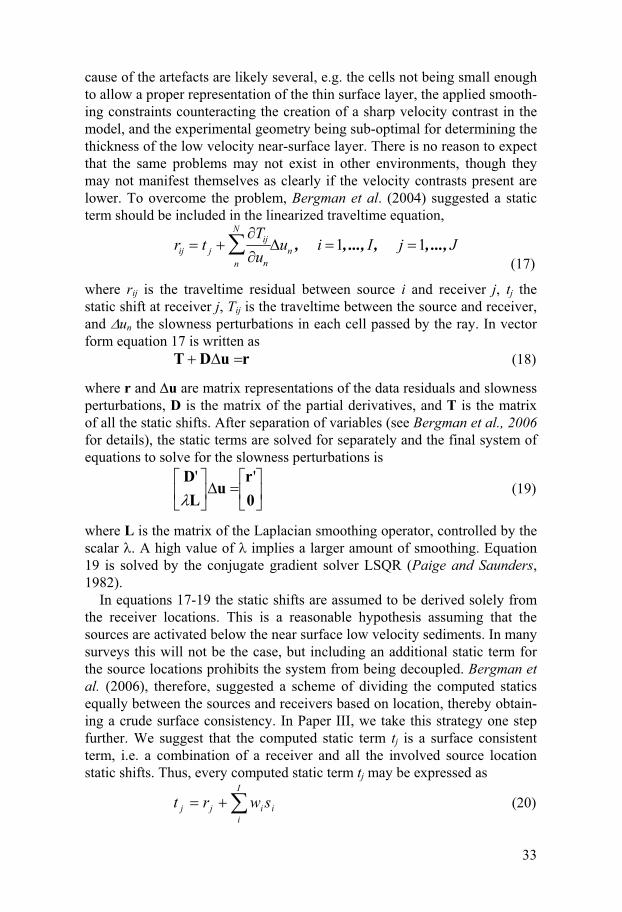
cause of the artefacts are likely several, e.g. the cells not being small enough to allow a proper representation of the thin surface layer, the applied smooth-ing constraints counteracting the creation of a sharp velocity contrast in the model, and the experimental geometry being sub-optimal for determining the thickness of the low velocity near-surface layer. There is no reason to expect that the same problems may not exist in other environments, though they may not manifest themselves as clearly if the velocity contrasts present are lower. To overcome the problem, Bergman et al. (2004) suggested a static term should be included in the linearized traveltime equation,
rij � t j ��Tij
�unn
N
� �un , i �1, ..., I , j �1, ..., J (17)
where rij is the traveltime residual between source i and receiver j, tj the static shift at receiver j, Tij is the traveltime between the source and receiver, and �un the slowness perturbations in each cell passed by the ray. In vector form equation 17 is written as
ruDT ��� (18)
where r and �u are matrix representations of the data residuals and slowness perturbations, D is the matrix of the partial derivatives, and T is the matrix of all the static shifts. After separation of variables (see Bergman et al., 2006 for details), the static terms are solved for separately and the final system of equations to solve for the slowness perturbations is
��
� !
"���
�
� !
"0r
uL
D ''
(19)
where L is the matrix of the Laplacian smoothing operator, controlled by the scalar . A high value of implies a larger amount of smoothing. Equation 19 is solved by the conjugate gradient solver LSQR (Paige and Saunders, 1982). In equations 17-19 the static shifts are assumed to be derived solely from the receiver locations. This is a reasonable hypothesis assuming that the sources are activated below the near surface low velocity sediments. In many surveys this will not be the case, but including an additional static term for the source locations prohibits the system from being decoupled. Bergman et al. (2006), therefore, suggested a scheme of dividing the computed statics equally between the sources and receivers based on location, thereby obtain-ing a crude surface consistency. In Paper III, we take this strategy one step further. We suggest that the computed static term tj is a surface consistent term, i.e. a combination of a receiver and all the involved source location static shifts. Thus, every computed static term tj may be expressed as
���I
iiijj swrt (20)
34
where rj is the receiver static term, si are all the I source static terms involved in computing tj, and wi is a weighting parameter (here we simply used 1/I for weights). Additional information may be the up-hole times (the vertical traveltime from the source to a receiver at the surface) if recorded, or a time shift computed from the datum differences between the sources and the re-ceivers and an assumed overburden velocity. In the present case no up-hole times were recorded since a surface source was used and the elevation dif-ferences between the sources and the receivers were generally small. The system of equations to solve may thus be written in matrix form as
��
� !
"��
� !
"��
�
� !
"sr
IIwI
pt
(21)
where, p contains the up-hole times (zeros in this case), the I’s are identity matrices, and t, r, w and s are the vector expressions of equation 20. The number of data and the number of parameters to solve for in equation 21 are equal, and r and s are solved for using SVD.
Inversion scheme In Paper III, the tomographic inversion scheme similar to the one of Berg-man et al. (2006) was performed over five iterations, gradually relaxing the weight on the Laplacian smoothing constraints ( in equation 19), in order to obtain a minimum structure model. Every iteration consisted of the follow-ing steps: 1) Forward computation of traveltimes and raypaths. 2) Simultaneous inversion for the velocities and the static shifts. 3) The computed statics are distributed between sources and receivers ac-cording to equation 21. 4) The new statics are applied to the data.
This sequence is repeated until a total root mean square (RMS) data misfit (including the statics) matching the estimated data error is obtained. Observe that the new statics are computed relative to the statics already applied. This provides a check for stability. If the statics oscillate, the solution is unstable.
4.3.2 Analysis of solution quality Estimating model resolution Two approaches are commonly used to assess solution robustness in traveltime tomography. The first approach assumes local linearity to esti-mate model covariance and resolution, the second tests resolution by recon-structing a synthetic model (e.g., a checkerboard test) using the same source-receiver geometry as the real experiment (Rawlinson and Sambridge, 2003). In practice, a checkerboard test involves inverting a set of synthetic traveltimes calculated for a model consisting of the background or final
35
model with an alternating pattern of positive and negative anomalies super-imposed on it. Then, the background or final model is used as the starting model, and the recovered model will closely resemble the checkerboard model in the well-resolved regions, but will elsewhere not resemble the checkerboard model. Thus, a measure of how well a region of the model is resolved is related to how well the known anomaly pattern is recovered (Zelt, 1998).
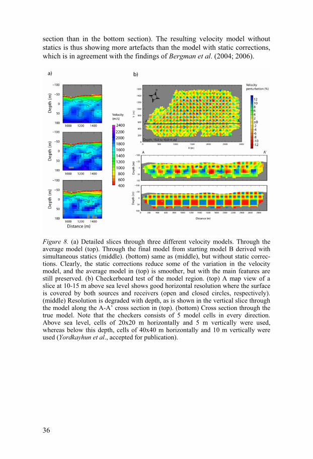
In Paper III, a series of synthetic model reconstruction tests, as well as tests with the real data, were performed to estimate the size of the model cells appropriate for the resolution power of the data set. The results on the real data showed that smaller cell sizes than 20x20 m horizontally did not improve the data fit. Checkerboard tests, however, indicated that this cell size does not represent the resolution of the data at all depths. A final check-erboard test with checkers consisting of 5 model cells in every direction is shown in map view and as a cross-section through the model (the top and middle in Figure 8b). The true model is also shown in Figure 8b (the bottom section). Judging from how sharp the corners of the checkers are recon-structed, the checkerboard test suggests that the resolution is on the order of 2 model cells, i.e. 40 m horizontally in the top of the model and about 80 m below 0 m depth. The vertical resolution is similarly estimated to 10 m and 20 m for the upper and lower model region, respectively. Model convergence and static corrections Generally, RMS data misfit is a crucial indicator how good the solution ob-tained is. However, the effect of the non-linearity of the problem makes it difficult to estimate the model reliability. This was found in Paper III where differences in the final models from the different starting models were ob-served, in spite of the similarity in RMS data misfit between the final mod-els. In order to mitigate the effect of the non-linearity, and to bring out the most significant (and stable) features of the model, the average of the 6 mod-els listed in Table 3, Paper III, were presented and interpreted rather than using the individual models. Although the averaging process can result in loss of real features and reduce resolution, averaging is also a robust tech-nique used in data processing for noise reduction.
Besides the overall RMS data misfit, the RMS static shift is also an indi-cator on model convergence and stability. In Paper III, the results showed that the RMS static shift shows no improvement after 5 iterations similar to the overall RMS data misfit. A comparison between the models along one of the profiles (Figure 8a) shows that the model derived with the static correc-tions (the middle section in Figure 8a) contains less wild velocity variations than the model derived without static corrections (the bottom section in Fig-ure 8a). The average model is shown for comparison in Figure 8a (the top section). Figure 8a also shows that some of the low velocity near-surface fill is absorbed in the static shift (near-surface velocities are higher in the middle
36
section than in the bottom section). The resulting velocity model without statics is thus showing more artefacts than the model with static corrections, which is in agreement with the findings of Bergman et al. (2004; 2006).
Figure 8. (a) Detailed slices through three different velocity models. Through the average model (top). Through the final model from starting model B derived with simultaneous statics (middle). (bottom) same as (middle), but without static correc-tions. Clearly, the static corrections reduce some of the variation in the velocity model, and the average model in (top) is smoother, but with the main features are still preserved. (b) Checkerboard test of the model region. (top) A map view of a slice at 10-15 m above sea level shows good horizontal resolution where the surface is covered by both sources and receivers (open and closed circles, respectively). (middle) Resolution is degraded with depth, as is shown in the vertical slice through the model along the A-A’ cross section in (top). (bottom) Cross section through the true model. Note that the checkers consists of 5 model cells in every direction. Above sea level, cells of 20x20 m horizontally and 5 m vertically were used, whereas below this depth, cells of 40x40 m horizontally and 10 m vertically were used (Yordkayhun et al., accepted for publication).
37
5. Overview of seismic reflection
2D and 3D high resolution seismic techniques have been increasingly ap-plied to the shallowest part of the earth in a broad range of objectives and with varying degrees of success. For instance, detection of fracture zones (Bergman et al., 2002; Schmelzbach et al., 2007), mapping of shallow aqui-fers (Buker et al., 2000; Francese et al., 2002; Juhlin et al., 2002; Zelt et al., 2006), investigating structure for geotechnical and engineering purposes (Steeples and Miller, 1990; Marti et al., 2002), etc. In applications for CO2 geological storage, studies elsewhere (e.g., Davis et al., 2002, Arts et al., 2004, Ziqiu and Takashi, 2004) have shown that time-lapse seismic tech-niques perform well in tracking the movement of CO2 in the subsurface.
Seismic reflection surveys routinely involve three basic parts: acquisition, processing, and interpretation. Intricate methodologies have been developed to acquire and process reflection seismic data. Since many conventional seismic exploration techniques are not suitable for shallow reflection seismic work, many of these methodologies are site and objective dependent. In this chapter, I point out some aspects of the seismic reflection method which are related to my research work. 5.1 Data acquisition Due to the current improvement of digital technology, the requirement of multichannel seismographs with a large dynamic range (Knapp and Steeples, 1986) is not the barrier to high resolution seismic surveys that it once was. The limitations are mainly controlled by the design parameters of sources and receivers and the field geometry, as well as costs. In particular, 3D seis-mic surveys have some level of compromise between technology and fi-nances. For 3D surveys, pre-planning tools or 3D seismic survey design programs were developed (Musser, 2000; Chaouch and Mari, 2006) and became a fundamental step to ensure that the 3D data quality will meet struc-tural, stratigraphy and lithology requirements. Generally, such survey de-signs concentrated on analysis of bin attributes and on offset sampling such as, regularity, fold, azimuthal distributions, etc. Experience from the 3D survey at the Ketzin site showed that it is possible to minimize the acquisi-tion cost by using a weight drop source, a relatively small number of chan-nels and a small field crew (Juhlin et al., 2007).
38
Choice of seismic sources The most site dependent part of the acquisition system is the energy source. An alternative to explosive sources, which are high-energy high-bandwidth sources but operationally expensive and subject to many environmental re-strictions, are vibrators on land (e.g. Woodward, 1994; Steer et al., 1996) and airguns at sea (e.g. Staples et al. 1999). Both sources have been used for reflection seismic profiling for petroleum exploration and deep seismic pro-filing. For small-scale surveys, a large number of land seismic sources have been developed and successfully applied to shallow engineering, groundwa-ter, mining and environmental problems (e.g. Pullan and MacAulay, 1987; Jongerius and Helbig, 1988; Steeples and Miller, 1990; Wright et al,. 1994). The choice of the most suitable seismic source depends on the target and the required penetration depth and resolution. Several studies have dealt with the essential aspects of sources through studying several factors, for example, site dependence and environmental conditions, energy and frequency con-tent, signal-to-noise ratio, source wavelet, repeatability, portability and eco-nomics. Obviously, in a 3D survey one might expect to acquire a large num-ber of shots over the area, the optimum cost, time, and portability are impor-tant factors that should not be neglected. The detailed information of source choices is described in Paper I which focuses on the comparison of the three seismic sources tested at the Ketzin site, including the VIBSIST, MiniVib and weight drop sources.
Bin size (Subsurface sampling) In 2D surveys, a good sampling of offsets in a CMP gather (or bin) is the main criterion of acquisition geometry. Similarly, in 3D surveys the general philosophy is extended from lessons learnt from 2D acquisition concerning the required binning of the recorded data in a common cell gather. The bin size will affect the lateral resolution of the survey. The required bin size is related to the signal sampling interval required to avoid aliasing. Aliasing can be neglected if the bin size satisfies (Yilmaz, 1987; Spitzer et al., 2001; 2003):
maxmax
min
sin4 �##�
fVb (22)
where b is the subsurface CDP bin size, Vmin is the minimum seismic veloc-ity to the target reflector, fmax is the maximum seismic frequency, and �max is the maximum dip to be imaged. In general, lower velocities, steeper dips, and higher frequencies will require smaller bin size for adequate spatial sampling of the higher frequency signals. For the Ketzin 3D data, the bin size is 12 m x 12 m and assuming the maximum dip of structures is 20o and minimum velocity of interest for the topmost reflector is 1500 m/s. Substitut-ing these values in the equation 22 yield the maximum unaliased frequency
39
expected, fmax of about 90 Hz which is close to the maximum useful fre-quency recorded.
Fold of coverage and offset distribution The fold represents the number of traces that are located within a bin and that will be summed during stacking. Source-receiver pairs have different directions. Traces within the bin thus have a range of azimuths and offsets but they correspond to the same subsurface location. When summed all traces carry the same signal, which is enhanced as it is in phase. However all traces have different random noise which is out of phase. The summation process decreases the level of noise. Then the fold contributes greatly to the enhancement of the S/N ratio. For comparable results between 2D and 3D data geophysicists used 3D fold as equal to half the 2D fold (Biondi, 2007). It should be noted that, for the shallowest interfaces, a reflection can often be observed on only a portion of the nearest offset traces, so that stack fold in reflection imaging is particularly low. This is the case encountered in the Ketzin data as well.
The fold of 2D surveys has a regular offset distribution. It contains an equal number of near, mid and far offsets. For 3D surveys the contribution of each class of offset is different; with a high percentage of far offsets, a small percentage of mid offsets and a very small percentage of near offsets (Chaouch and Mari, 2006). So a large number of far offsets will improve the suppression of multiples, whereas a small number of near offsets will reduce the noise associated with this class of offsets such as ground roll, air blast, source generated noise, etc. This will result in an improvement in the S/N ratio.
5.2 Data processing The aims of seismic data processing are to enhance the S/N ratio and the resolution of the data so that the final image resembles as closely as possible the true geological structures. Despite complicated by the fact that a typical 3D survey contains more data to process, the actual processing steps are fairly similar to those for 2D surveys. Data processing of shallow profiles require particular attention to near-surface problems associated with resolu-tion and velocity analysis, refraction arrival muting and source-generated noise suppression. These considerations have been emphasized in the data processing description presented in Paper IV. 5.2.1 Static corrections Static correction are the time shifts that have to be applied in order to let the seismic record appear as if it had been recorded with shot and geophone at a
40
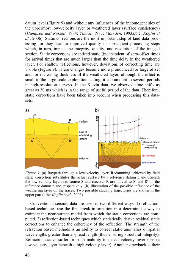
datum level (Figure 9) and without any influences of the inhomogeneities of the uppermost low-velocity layer or weathered layer (surface consistency) (Hampson and Russell, 1984; Yilmaz, 1987; Marsden, 1993a,b,c; Koglin et al., 2006). Static corrections are the most important step of land data proc-essing for they lead to improved quality in subsequent processing steps which, in turn, impact the integrity, quality, and resolution of the imaged section. Static corrections are indeed static (independent of zero-offset time) for arrival times that are much larger than the time delay in the weathered layer. For shallow reflections, however, deviations of correcting time are visible (Figure 9). These changes become more pronounced for large offset and for increasing thickness of the weathered layer, although the effect is small in the large scale exploration setting, it can amount to several periods in high-resolution surveys. In the Ketzin data, we observed time shifts as great as 30 ms which is in the range of useful period of the data. Therefore, static corrections have been taken into account when processing this data-sets.
Figure 9. (a) Raypath through a low-velocity layer. Redatuming achieved by field static correction substitutes the actual surface by a reference datum plane beneath the low-velocity layer, i.e. source S and receiver R are moved to S' and R' on the reference datum plane, respectively. (b) Illustration of the possible influence of the weathering layer on the traces. Two possible stacking trajectories are shown in the upper part (after Koglin et al., 2006).
Conventional seismic data are used in two different ways. 1) refraction-based techniques use the first break information in a deterministic way to estimate the near-surface model from which the static corrections are com-puted. 2) reflection-based techniques which statistically derive residual static corrections to enhance the coherency of the reflection. The strength of the refraction based methods is an ability to correct static anomalies of spatial wavelengths greater than a spread length (thus ensuring structural integrity). Refraction statics suffer from an inability to detect velocity inversions (a low-velocity layer beneath a high-velocity layer). Another drawback is their
41
inability to resolve thin beds (known as the hidden layer problem), and the interpretation of velocity increases with depth within a layer can be prob-lematic with some implementations.
Often, after applying refraction statics, the section is still noisy. This is typical and is due to residual anomalies left by imperfections in the model. Thus, the surface consistent residual techniques lay in statistically adjusting the shorter wavelength anomalies remaining in the individual gather after the other techniques had been applied.
5.2.2 Effects of source-generated noise The shallowest reflections are often obscured by near-surface refractions, coherent and random noise, which must be removed in order to analyse the reflection moveout prior to the NMO correction and stacking (Feroci et al., 2000). Typically, there are three types of linear events in the time-offset (t-x) domain: direct and refracted body waves, the ground-coupled sound wave (air blast) and ground roll. The ground roll masks reflections at small offsets, while refracted arrivals occur for larger offsets and specifically affect shal-low reflections. The interaction of the air blast with body wave events de-pends strongly on the velocities of the body waves. For unconsolidated or dry material the velocities of the body wave may be only slightly higher than the velocity of the air blast and the distorted area is found in the middle of the zone that also shows reflections. For consolidated (or water-saturated) sediments the velocity of body waves is usually much higher than that of the air blast velocity, thus the air blast predominantly affects the S/N ratio at small offsets (Brouwer and Helbig, 1998). Note that S-wave velocities may be even significantly lower than the velocity of the air blast.
MutingTrace muting is the removal of parts of the traces (Miller, 1992). Standard reasons for muting are interference of strong first arrivals, ground-coupled air waves, and surface waves. Trace mutes are used as top mutes (refracted arrival and direct wave), bottom mutes (surface wave or ground roll), and surgical mutes (air blast). Mute have to be tapered to avoid abrupt changes which is harmful in the Fourier analysis of the trace. Muting may not be the first option of coherent noise removal since not only noise is removed, also reflection information is excluded. However, in particular cases it may be necessary when the other processes do not perform well. For example, f-k filtering which is a popular tool to suppress refraction events is somewhat limited in the processing of shallow seismic data. This is due to the side ef-fects caused by the f-k filter highly distorting the data, aliased noise remains after the filter application and the distinction between noise velocities and signal velocities may only be small.
42
5.2.3 Velocity analysis and NMO correction The aim of velocity analysis is to find the velocity that flattens a reflection hyperbola, which returns the best result when stacking is applied. Moreover, a good velocity model is the basis for appropriate time-to-depth conversion and migration. By making the small spread approximation (maximum offset smaller than the maximum target depth), for a horizontally stratified me-dium, the travel time equation tx for a wave reflected on a layer associated with the normal incident travel time t0 is:
2
220
2
NMOx v
xtt �� (23)
where x is the source – receiver offset, t0 is the normal incident travel time, and vNMO is the NMO (or stacking) velocity. The traveltime curve associated with the reflected wave is a hyperbola given by the equation. A NMO cor-rection, �tNMO is computed for each trace at offset x and subtracted from the recorded time tx. This operation transforms each tx to an equivalent normal incident travel time t0:
20
2
0 2 NMOxNMO vt
xttt $��� (24)
The NMO correction depends on offset and velocity (Bradford, 2002). The velocity, vNMO required for the NMO correction for a horizontally strati-fied medium is equal to the rms velocity. The stacking velocities obtained by conventional velocity analysis may deviate greatly from the rms velocities of the earth model which they are assumed to approximate, particularly in the shallow section, although the discrepancy between the two sets of values decreases with depth. When reflectors dip then vNMO is not equal to the ac-tual velocity, but dependent upon the dip. Stacking velocities are biased by a factor proportional to the inverse of the cosine of the apparent dip. In this case the velocity bias is removed after application of DMO (Biondi, 2007; Schmelzbach et al., 2007).
The accuracy of velocity analysis, therefore, is influenced by many fac-tors, such as S/N ratio, depth and dip of reflector, and static correction, etc. Static corrections and velocity analysis are closely linked to each other (Marsden, 1993c). Every time a set of static corrections is computed and applied to the data, the origin of the data (i.e., zero time) is moved for veloc-ity analysis purposes. So, for those techniques where analysis takes place after the application of an NMO correction, it becomes necessary to reana-lyze the velocities after each iteration since the quality of the stacked section is affected.
As the velocity usually increases with time, the NMO hyperbola becomes flatter and flatter at longer offsets. Thus, for any offset, the time difference between two hyperbolae is smaller than the corresponding time difference at
43
zero-offset. After the NMO correction, a wavelet with a dominant period T is stretched and becomes a wavelet with a dominant period TSTR larger than T. Stretching is quantified by a stretching factor � (expressed in percentage, Yilmaz, 1987):
0tt
ff NMO�
��
�% (25)
where f is dominant frequency associated with the dominant period T and �f is the change in frequency. Thus, loss of the high frequency components of the amplitude spectrum may be introduced by the stretching. Although NMO stretch muting (Miller, 1992) reduces this frequency distortion, the stacking fold for shallow events also reduces. Thus, this parameter must be optimized as shown in Paper IV.
5.2.4 Time-to-depth conversion When the subsurface is horizontally stratified, the reflections from flat inter-faces are still described well by hyperbolas, but the stacking velocity varies according to the depth of the interface. That is the stacking velocity is a function of the two-way-traveltime to the apex of the hyperbolas. The stack-ing velocity function is an average velocity, and it cannot be used directly to transform two-way-traveltimes into depth. To convert time to depth, one estimates the mapping velocity function, that is, the propagation velocity or interval velocity (Biondi, 2007). Traveltime-to-depth conversions can be unreliable because of either inaccurate velocity control or incorrect event identification. For simple geological structures (e.g., nearly horizontal layer-ing), the seismic ray paths can be assumed to be vertical, and time-to-depth conversion is a mere exercise in multiplying interval times by interval ve-locities. The interval velocities can either be obtained from well information or calculated from the stacking velocity profile using the Dix formula (Dix, 1955).
2/1
1
12
1,2
, )()(���
����
�
�
��
�
��
nn
nnrmsnnrmsi tt
tVtVV (26)
where
��
��n
iin tt
1is the total two-way traveltime to the bottom of the nth layer.
Once the interval velocity is known, the time-to-depth conversion is de-fined by the transformation
��
��j
iiij tVz
121
(27)
44
where zj is the depth at the bottom of the Jth layer.
Velocity estimation needs to be more accurate when working on the small scale or at shallow depth. In determining interval velocities Dix assumes that the stacking velocity can be described by the rms velocity (which is not gen-erally true as mentioned before). Furthermore, the determination of interval velocities is rather sensitive to errors in stacking velocity. A general over-estimation or underestimation of velocities lead to small errors in interval velocity, whereas alternating errors in stacking velocity may yield highly unrealiable interval velocities and depths (Bradford, 2002).
5.3 Data interpretation Interpretation is concerned with the qualitative and quantitative reconstruc-tion of the subsurface from the intermediate results of processing, generally in terms of the specific problem at hand. Following Badley (1985) seismic interpretation generally assumes that; (1) the coherent events seen on the seismic records or on seismic sections are reflections from acoustic imped-ance contrasts in the earth, (2) these contrasts are associated with boundaries that represents geologic structure, and (3) seismic detail (e.g., wave shape, amplitude, etc.) is related to geologic detail.
The inclusion of external geological and geophysical constraints is often the key to successful interpretations and the development of a reasonable subsurface geologic image. Several boreholes drilled in conjunction with the natural gas facility and groundwater studies at the Ketzin site proved to be useful information in aiding interpretation as shown in Papers III and IV. Seismic attributes and seismic modeling are the other interpretation tools I used in Paper IV.
Seismic modeling Seismic modeling is a technique for simulating wave propagation in the earth (Carcione, et al., 2002). The objective is to predict the seismogram that a set of receivers would record, given an assumed structure of the subsur-face. This technique is a valuable tool for seismic interpretation and an es-sential part of seismic inversion algorithms. Another important application of seismic modelling is the evaluation and design of seismic surveys. There are many approaches to seismic modelling, such as finite-difference, finite-element, ray tracing, Gaussian beam and Kirchhoff modeling. In Paper IV, finite-difference modeling (Juhlin, 1995) was used to study the lateral varia-tion in impedance contrast at the base of the Quaternary sedimentary unit.
The major use of synthetic seismograms is to compare them with actual seismic data in order to identify reflections associated with particular inter-faces, so that maps can be made on the bed of particular interest. Seismic
45
sections often contain phase shifts of unknown magnitude, so that the ability to match synthetics to actual data adds considerable confidence to an inter-pretation.
Seismic attribute and neural network as aids in interpretation Seismic attributes, including measures of seismic amplitude, frequency, and phase, have been used successfully in mapping seismic lithology changes (Marfurt et al., 1998; Chopra and Marfurt, 2005). However, many attributes available are not independent pieces of information but, in fact, simply rep-resent different ways of presenting a limited amount of basic information. The key to success lies in selecting the most applicable attribute for the prob-lem. For example, when there is sufficient lateral change in acoustic imped-ance, the 3D seismic coherency attribute can be extremely effective in de-lineating seismic faults, quantifying the seismic discontinuities at each point in the volume. Discontinuities that are attributable to fault surfaces include dip, azimuth, and offset changes of seismic reflectors, and waveform and amplitude variations caused by defocusing (Cohen et al., 2006). Such dis-continuities appear on coherence slices as incoherent linear or curved fea-tures. The problem is that there is no perfect fault attribute, but many attrib-utes can contribute to fault interpretation. To handle this situation, the semi-automatic approach to seismic object detection, uses multi- and directive attributes (i.e., attributes that are extracted in data-steered directions, mean-ing that the attribute response is calculated along the seismic reflection en-ergy that forms geologic horizons) and neural networks to highlight objects of interest based on interpreter’s insight which is incorporated in the process in the form of handpicked fault and non-fault positions (Meldahl et al., 2001; Tingdahl and de Rooij, 2005). The method was initially applied to highlight seismic chimneys for the interpretation of hydrocarbon migration paths (Heggland et al., 1998; Tingdahl and de Groot, 2001). The same methodol-ogy can be used to detect other seismic objects, such as salt bodies, fractures, reflectors and bright spots. In Paper IV, this method was applied for fault detection in the 3D volume with a certain degree of success.
46
6. Summary of the papers
This chapter presents a summary of the four papers which are the basis of this thesis. In each paper, the main objectives, methodology and results are briefly described, followed by the conclusions. The papers are the result of a team work and credits are given to my co-workers. The theoretical back-ground, methodology and interpretation of the results were significantly improved through the intensive discussion with my co-authors. Apart from the field work and writing of the manuscripts, my contributions in each pa-per varied. In Paper I, the study was done by me, except the processing of the MiniVib and weight drop data. In Paper II, the study was done by me and the interpretation of the results was done together with my co-authors. In Paper III, the tomography inversion was performed by me and my co-authors assisted in the checking of solution quality, methodology and as-sisted in the interpretation. In Paper IV, processing of the seismic reflection data, seismic modeling and seismic attribute analysis were done by me and the interpretation of the results was done together with my co-authors.
6.1 Paper I Comparison of surface seismic sources at the CO2SINK site, Ketzin, Germany
6.1.1 Summary The objective of this paper was to compare the three seismic sources tested in the pilot study: VIBSIST, MiniVib and weight drop. In this study, we compare the apparent S/N ratio, penetration depth and frequency content using individual source gathers, followed by comparisons of stacked sections along two different test lines. Finally, the advantages and disadvantages of the three different sources are discussed.
To avoid contamination from the high amplitude air wave and ground roll, the seismic traces in the “optimum window” (offset interval 1000-1200 m) in the raw shot gathers were used for signal penetration and frequency content analyses. For comparison of seismic sections, we have focused our data processing and analysis on the upper 1.5 s since the target horizon for the CO2SINK project is at about 700 m depth. Several conventional process-
47
ing steps were applied in order to enhance the data in the upper 1.5 s (see Table 3 in Paper I). Given the differing nature of the sources, each data set was processed independently of the others when producing stacked sections.
Following Staples et al. (1999) and Benjumea and Teixido (2001), the ap-parent S/N ratio was calculated. The analysis was performed on common-offset gathers using stacked traces of five adjacent shots within the selected offset range. The average apparent S/N ratios of the VIBSIST, MiniVib and weight drop sources within this analyzed offset range are 5.58, 4.70 and 5.30, and their standard deviations are 1.82, 0.98 and 1.74, respectively. The S/N ratio of the VIBSIST and weight drop data is relatively higher than the MiniVib data, but they appear to have a larger variation than the MiniVib data (Figure 10a), implying that the MiniVib source may have the better repeatability.
The signal penetration of the VIBSIST, weight drop and MiniVib sources were compared in a quantitative manner by studying the amplitude decay curves. To perform this analysis, the absolute amplitudes of the traces from five adjacent shots were used. These traces were then stacked by taking the mean values of all traces in this offset range to form a single trace for each shot. Stacked traces from five adjacent shots were then averaged to obtain a master trace. Average amplitudes of this trace were then calculated for 100 ms time windows from 0 to 1.5 s. Given that the first arrival is at about 500 ms in this offset range, the amplitude values from the first to the fifth time windows represent background (ambient) noise levels. The MiniVib data show the highest peak amplitude in the first arrival time window, whereas the amplitudes of the VIBSIST data and the weight drop data are lower, sug-gesting that the MiniVib is putting the largest amount of energy into the ground. However, if amplitude is normalized to peak amplitude for each source (Figure 10b) the amplitude decay curves differ after the 700 ms time window. Normalized amplitude decreases more slowly for the VIBSIST data, suggesting that this source has the greatest penetration.
Amplitude spectra for each source are shown in Figure 10c. All three sources have dominant signal frequencies of around 30-120 Hz (> 2 oc-taves), providing enough bandwidth for resolving the geological target. The high frequency portions of the amplitude spectra differ for the three sources. The amplitude spectrum of the MiniVib is controlled by the frequencies of the signals put into the ground, 30-150 Hz. Amplitudes outside this range for the MiniVib should be regarded as noise. No upper limit exists for the fre-quencies of the signals put into the ground by the VIBSIST source, however, the VIBSIST data were wide-band filtered to improve S/N ratio before ap-plying the shift and stack process. The falloff in amplitudes at high frequen-cies reflects this pre-processing step. Weight drop amplitude spectra from time windows prior to the first arrival show a flat spectrum, similar to that shown in Figure 10c. This proves that no useful energy is put into the ground by the weight drop at frequencies greater than 150 Hz. Even the low ampli-
48
tudes in the frequency range 100-150 Hz are indicative that it is mainly noise that is recorded at these frequencies by the weight drop source.
Figure 10. a) Apparent signal-to-noise ratios of the three different sources at se-lected offsets. b) Signal penetration of the three seismic sources by comparing nor-malized amplitude with traveltime. c) Amplitude spectra of the three seismic sources.
49
The sections from all three sources (Figure 11) show the major reflections corresponding to the lithologic setting in the area. Line 1 is characterized by overall lower S/N ratio compared to Line 2. All sections from Line 2 show clear reflections down to 1.4 s. In Figure 11 the deepest reflector (1.3 s to 1.4 s) is characterized as a nearly continuous event along all CMPs, showing the higher signal energy transmitted by the VIBSIST source. A more detailed signal analysis with respect to the target horizons is shown in Figure 11 in Paper I. In this time window (0.35 s to 0.7 s) the reflection signals of the MiniVib data show higher frequencies (higher resolution) than the signals of the VIBSIST data and of the weight drop source. The transmitted signal energy of the three sources is high enough to image the reflections from the L4 to K2 reflectors at all CMPs. Below the K2 reflection the MiniVib data show less continuity (e.g. K3 reflector, CMP 660 to 685 in Figure 11, Paper I) than the two impact sources.
6.1.2 Conclusions The three seismic surface sources are characterized with respect to their S/N ratios, signal penetration and frequency content by analysis of raw shot gath-ers and by examination of stacked sections along two lines within the planned 3D seismic area at the Ketzin site. The results showed that: 1) Near surface conditions strongly influence the signal bandwidth (resolu-tion) and signal energy. This is expressed by the difference in reflectivity of the two CMP lines. 2) The CMP sections of the MiniVib source show the largest amount of high frequency signals to about 500 ms (~500 m depth), but the shallowest signal penetration. The VIBSIST source generates signals with the highest S/N ratio and greatest signal penetration of the tested sources. In particular, the reflections below 900 ms (~1 km depth) are best imaged by the VIBSIST source. In terms of S/N ratio and signal penetration, the weight drop per-formance is in between the other two sources. Apart from the source-generated noise encountered at near offset traces for all three sources, ambi-ent noise is higher at far offsets on both the MiniVib and weight drop data. At the cost of increased acquisition time, this noise could possibly be re-duced by increased vertical stacking. 3) Since all 3 sources imaged the target horizon, the choice of source for the 3D survey (Juhlin et al., 2007) was based mainly on logistics and cost. Given that time was an important factor, the weight drop source was recom-mended as the primary source for the 3D survey. For future monitoring pur-poses within the project framework, 2D data were acquired using the VIB-SIST source (Juhlin et al., 2007).
50
Figure 11. Stacked sections and fold plots of Line 2. (a) VIBSIST section, (b) Mi-niVib section and (c) Weight drop section. T1= near base Tertiary, L4 = top Triassic (assumed), K2 = top Weser Formation, K3 = near top of Grabfeld Formation.
51
6.2 Paper II Shallow velocity-depth model using first arrival traveltime inversion at the CO2SINK site, Ketzin, Germany
6.2.1 Summary The aims of this study were: 1) joint interpretation of refraction and reflection seismic data in order to obtain information on near surface structures (e.g. shallow aquifers, thick-ness of the cover). 2) to improve the time-to-depth conversion of the seismic reflection sections.
First arrival traveltime inversion proposed by Hampson and Russell (1984), the generalized linear inversion (GLI) method, was used to produce the velocity-depth models. The method is described in Chapter 4. Picked first arrival traveltimes from shots by the weight drop source from the pilot 2D reflection seismic data were used as input in this study. Stacked sections from the VIBSIST source as presented in Paper I were compared in inter-preting the resulting velocity-depth models.
The inversion method was tested by using different initial uniform lay-ered models in order to investigate the influence of the initial guess. After several tests, it was decided to use five layers for the initial model.
The velocity-depth models for Line 1 and Line 2 are quite similar, con-sisting of a sequence of uniform layers, except for the differences in geome-try. The velocity-depth models for both profiles are fairly homogeneous laterally, and velocity increases slowly with depth.
The depth converted sections (unmigrated) obtained for Line 1 and Line 2 using (1) the stacking velocity from the CDP processing (solid line in Figure 12) and (2) the velocity-depth models obtained in this study (dashed line in Figure 12) were compared (Figure 13). The depths to the reflections ob-tained using the GLI velocity model are different than the depths obtained using the stacking velocity, implying a discrepancy between the two velocity functions. The Dix interval velocity of the upper 500 m and the GLI veloc-ity-depth model of Line 1 and Line 2 are compared in Figures 12. In the upper 300 m there are only small differences in the interval velocities, but the layer boundaries of the GLI velocity model are somewhat shallower than the Dix velocity model from the CDP processing. Moreover, in the upper 150 m, only one layer is present in the Dix velocity model, while two layers are observed in the GLI velocity-depth model. Below 300 m, velocities in the Dix velocity are higher than in the GLI model. By analysis of RMS error and ray coverage, layer velocities and geometries are less accurate for the deeper layers in the GLI model. Therefore, the Dix model may be more reli-able below 300 m.
52
In order to compare the GLI models directly with the reflection seismic sections they have been superimposed on top of the depth sections (Figure 13). It is obvious that layer boundaries as defined by clear reflections on the seismic sections are more consistent with velocity boundaries from the GLI models obtained when using the velocity-depth models from this study com-pared to using the Dix velocities for depth conversion. This result indicates that use of the GLI velocity fields produces a better time-to-depth conversion of the reflection data, at least in the upper 300 m. It should be noted that some reflectors have not been detected in our models (reflectors within the yellow zone in Figure 13a and 13b). This is probably due to (1) there is a possible fault zone between position 600-1200 m in Line 1, where the rays pass through a complex structure and (2) GLI is solved by a ray based ap-proach, implying the ray path is biased to high velocity layers whereas the reflections may be due to low velocity zones. Correlation is better between layer boundaries where the reflector is clear (arrow marked at about 350 m depth in Figure 13b).
Figure 12. Velocity function used for time to depth conversion of (a) Line 1 and (b) Line 2. Solid line is the Dix velocity function and the dashed line is the GLI velocity function.
Thick near surface low velocity layers are problematic, both when invert-ing for the velocity-depth model and when processing the reflection seismic data, particularly Line 1. The poorer model restoration obtained on Line 1 is probably due to statics problems associated with the topographic high con-taining low velocity material. The significant decrease in the RMS error on Line 1 after inclusion of the short-wavelength static calculation is evidence for this. This suggests that solely using refraction based static corrections is not adequate and that improvement in the section can be obtained using a surface-consistent static method for handling short wavelength variations (residual statics) in the reflection seismic processing.
53
Figure 13. Depth section overlain by the GLI model of Line 1 (a and b) and Line 2 (c and d) using the Dix velocity (top) and the GLI velocity (bottom). Orange arrows mark examples of locations where the correlation between the depth section and the GLI model is better than with the Dix velocities. Geologic interpretation is con-strained by information from the Ktzi 169/63 borehole.
Geological interpretation based on the combination of our models, the re-flection seismic sections and data from the Ktzi 163/69 deep borehole show that the upper 400 m of the subsurface are represented by four groups of sediments. In general, the uppermost layer consists of low velocity (1000 m/s) unconsolidated sediment with a thickness varying from 5 m where to-pography is fairly flat to 15-30 m where topographic relief is high. Quater-nary sandstone deposits with velocities of 1600-1700 m/s and 50-110 m thick are present below these unconsolidated sediments. The velocities sug-
54
gest saturated soil material in a shallow aquifer as the composition of this layer. This unit is underlain by Tertiary deposits of mudstone with velocities of about 1950-2050 m/s and thickness ranging from 60 to 120 m. Below the Tertiary unit, Jurassic sedimentary sequences are represented by an alternat-ing sequence of sandstone, mudstone and siltstone extending to depths of about 250-400 m and with velocities in the range of 2300-2600 m/s.
6.2.2 Conclusions 1) A more detailed picture of the uppermost 200 m is obtained. The sedi-mentary units are characterized by a gradual increase in velocity with depth with lateral velocity variations being insignificant. 2) The velocity-depth models may also be used to convert the reflection seismic sections from time to depth. Compared to using stacking velocities, the GLI velocity model based depth sections provide a more consistent im-age of the subsurface. 3) The GLI method allows for the calculation of short and long wavelength statics which can be used to improve the reflection seismic processing. 4) Some limitations in the method should be noted including: thin layers or low velocity layers (the hidden layer problem), the inherent non-uniqueness of traveltime inversion (dependent on the quality of the picked first arrivals, choice of initial model and the degree of near-surface lateral velocity varia-tions) and a priori information is required to increase the confidence level of the final solution.
6.3 Paper III 3D seismic traveltime tomography imaging of the shallow subsurface at the CO2SINK project site, Ketzin, Germany 6.3.1 Summary The objectives of this study were: 1) to test for 3D traveltime tomography inversion reliability in a sedimentary environment by using a tomography with statics algorithm. 2) to obtain a better image of the near surface, especially the internal struc-ture of Quaternary sediments, where the seismic image in the upper 150 ms in Juhlin et al. (2007) was not well resolved. 3) to track the extension of major faults towards the surface and possible residual gas upward migration along these faults.
The PStomo_eq (Tryggvason et al., 2002) algorithm was used for tomo-graphic inversion. A detailed description of the algorithm is provided in Chapter 4.
55
A series of starting models were tested on a small data set, ranging from constant velocity layers and layers with different gradients to a constant gra-dient model. After the optimum starting model was selected, further tests with variations on this starting model were done on the full data set.
Given the results of model assessments described in Chapter 4, the aver-age tomographic model was chosen for interpretation. This model is pre-sented in the form of cross sections and depth slices to display the velocity variations in 3D (see Figures 14-16). In general, the models show gradually increasing velocities with depth and strong lateral velocity variations, espe-cially in the eastern part of the study area, indicating a heterogeneous subsur-face.
Boreholes located near each profile in Figure 14 allow for direct compari-son of the velocity model with lithological boundaries. The images show several coherent structures along the profiles. The low velocity (800-1200 m/s) near-surface layers represent the uppermost unconsolidated material consisting mostly of sand. The thickness of this layer varies from near 0 m up to 20 m in regions of high topography. The boundary between the Qua-ternary unit and the Tertiary clay unit, which was not mapped in the seismic reflection volume presented in Juhlin et al. (2007), is identified on the basis of where the velocity reaches ~1800 m/s at a depth of approximately 60-80 m below the surface (Figure 14). Although this boundary does not correlate one to one with the borehole observations, the general trend of the transition correlates. Velocities in the range of 1600-1800 m/s probably represent variations in the internal structure of Quaternary unit and may indicate changes in its aquifer properties. The higher velocities (> 1800 m/s) at some locations in the upper part of this unit are interpreted to reflect the local oc-currences of glacial till. These tills may act as aquitards within the main aq-uifer of this unit. These shallow high-velocity features may also bias the ray paths and are a significant obstacle to traveltime tomography since the ray density will decrease in the deeper layers below these units.
Significant lateral velocity variations are also present in the Tertiary clay unit (velocities above 1800 m/s, below 50 m depth). Possible reasons for these lateral velocity variations include (1) lateral variations of lithology within the unit, (2) deeper faults extending into this unit, (3) alteration within the unit due to fluid/gas migration along more deep seated faults, and (4) artefacts from the tomography. Therefore, it is possible that the low veloci-ties in the Rupelton clay may be due to alteration associated with the fault zones, even if the fault zones do not extend into the unit. Support for this interpretation is found in that these low velocity zones roughly coincide in our model with the extrapolation of the fault zones interpreted in the 3D reflection seismic volume and are marked by arrows in Figure 14.
Figure 15 shows selected south-north stacked sections from the 3D reflec-tion seismic volume (Juhlin et al., 2007) overlain by the corresponding to-
56
mography sections. These images also indicate a correlation between the low velocity patterns with the fault trends in the 3D reflection seismic volume.
Figure 14. West-east oriented tomographic cross sections (vertical slices) overlain by geological data from nearby boreholes. Locations of the cross sections are shown on the index map. Regions undersampled by the rays are masked. Arrows indicate locations of interpreted faults below the Tertiary unit based on similarity attribute maps of the 3D reflection seismic volume (Kazemeini et al., 2008). Dashed line highlights the possible Quaternary/Tertiary boundary. Depth is measured relative to sea level and vertical exaggeration is 3:1.
Our tomographic models help to fill the poorly resolved uppermost 100 m of the survey area in the reflection seismic images. Moreover, the tomo-
57
graphic image shows general agreement with the shallow velocity-depth model down to 100 m from the 2D pilot data (Yordkayhun et al., 2007) and provides us with a more detailed velocity structure (Figure 15d and 15e). This is due to the smoothness constraints imposed on the latter.
Figure 15. (a) to (c) show south-north slices from the 3D reflection seismic volume overlain by the tomographic cross sections shown in the index map. Red lines indi-cate interpreted faults based on the 3D reflection seismic volume. (d) and (e) com-pare a tomographic cross section that is coincident with the shallow velocity-depth model obtained from the 2D pilot data (Yordkayhun et al., 2007).
In order to emphasize the fault zones and their possible extension into the near surface, the fault trends from seismic amplitude analysis near the base Tertiary have been compared with our results. In the tomography depth
58
slices at 45-80 m (about 85-130 m depth below surface), some of the fault zones can be associated with low velocity anomalies striking mainly in the east-west direction (Figure 16). Anomalies A1 and A2 mark possible exten-sions of the deeper mapped faults into the Tertiary Rupelton clay, whereas anomaly A3 marks a possible altered rock volume associated with other fault zones. Of the three anomalies, it is the A1 anomaly that correlates most clearly with a mapped fault and the anomaly can be traced in a consistent manner to different depth slices within the Tertiary unit (Figure 16).
It is not possible to determine if the residual gas has migrated into the Tertiary clay based on the tomographic results. Presumably the geological structure will be well mapped and the location of faults well known prior to large scale storage of CO2 at a given site. Seismic refraction tomography could then play a role in monitoring the near surface in the vicinity of the faults.
6.3.2 Conclusions 1) The first-arrival times picked from the 3D reflection seismic data can be used to obtain reliable information on the velocity structure shallower than about 150 m below the surface. 2) Clear features which can be identified from the resulting velocity models are as follows: & A low velocity layer of 800-1200 m/s covers this area down to depths as
great as 20 m below the surface where the topography is high. & The internal structure of the Quaternary aquifer unit is characterized by
velocities of 1600-1800 m/s and this unit is inter-layered at some loca-tions by relatively high velocities that may correspond to thin layers of glacial till that act as aquitards within the main aquifer. These thin high velocity layers are the main obstacle to traveltime tomography in the area since they prevent rays from penetrating to deeper levels.
& In regions where the sub-surface velocity is relatively homogeneous, the Quaternary-Tertiary boundary is imaged in the depth range 60-80 m, co-inciding with the 1800 m/s iso-velocity horizon.
& Fault zones interpreted from the 3D reflection seismic images generally project into the tomographic image where low velocity anomalies are pre-sent or the volume is undersampled by rays below 100 m depth. This ob-servation suggests that some of the fault zones may extend into the Terti-ary section.
3) Although the tomographic images alone are not able to determine if any of these low velocity zones contain residual gas escaping along the faults from the deeper Jurassic formations, the results show that refraction tomo-graphy is a potentially useful tool for investigating and monitoring of CO2 geological storage sites.
59
Figure 16. Tomographic depth slices at selected depths. Bottom slice shows similar-ity attribute map at 150 ms (after Kazemeini et al., 2008). The clear near-linear fea-tures in the similarity map are interpreted as representing fault zones and their gen-eral geometry are shown as solid lines in the figure. Shots and receivers are marked by dots and triangles, respectively. The regions undersampled by ray paths are masked. A1, A2 and A3 show the location of low velocity anomalies that are dis-cussed in the text.
60
6.4 Paper IV 3D seismic reflection surveying at the CO2SINK project site, Ketzin, Germany: A study for extracting shallow subsurface information
6.4.1 Summary The objectives of this study were: 1) to enhance the Quaternary-Tertiary horizon and shallow structures associ-ated with the major fault zones by reprocessing a subset of the 3D data. 2) to combine the results from the reprocessed subset of data, shallow bore-hole information, the tomography study and hydrogeology information into an integrated interpretation of the uppermost 200 m.
The 3D seismic data acquisition procedure is described in detail in Juhlin et al. (2007) and the main parameters are summarized in Table 3 in Chapter 2. Data from 2 swaths located over the fault zone area were extracted from the entire 3D volume and were truncated to a maximum traveltime of 400 ms and a maximum offset of 400 m. The processing sequence for this data sub-set is outlined in Table 2 in Paper IV and a detailed description of the most important steps is provided as follows. & More accurate 3D refraction statics were recalculated using a near-surface model obtained from all first arrival times picked on all offsets up to 400 m. Moreover, the residual moveout was taken into account. We demonstrated that 10% of the residual moveout with respect to the surface can be ac-counted for by moving the datum 10 m down from the surface. & Given the trade-off between CMP bin size and frequency content, the data were bandpass filtered at 30-100 Hz after deconvolution. & A mute function containing the entire noise cone of ground roll performed best as a tail mute. Carefully designed top mutes were used to eliminate di-rect and refracted waves from CMP gathers and a 100% stretch mute was used in the NMO correction. & The final velocity function used for NMO corrections was updated after the velocity analysis-residual static corrections cycle. This velocity function proved to be appropriate for migration and time-to-depth conversion. & The coherency enhanced stacked volume was migrated to collapse dif-fractions and to improve lateral resolution.
In the upper 300 ms, the integration of a sequence of time slices, in-lines and cross-lines from the migrated 3D volume, shallow borehole information, tomographic images, and hydrogeologic information allow structures to be identified reliably. The main reflecting boundaries have been mapped semi-automatically on the basis of their characteristic seismic response, including (from top to bottom) the near base Quaternary (BQ), near base Tertiary (de-fined as T1 horizon, Reinhardt, 1993), near Top Sinemurian (TS) and the upper and lower gas layers (G1 and G2) (Figure 17).
61
The topmost horizon, the estimated boundary between the Quaternary sediments and the Tertiary clay unit, is now found at about 95-120 ms. Cor-relation between shallow boreholes and the migrated depth volume confirms the presence of this boundary at about 65-90 m depth (Figure 17b). The ver-tical resolution is about 4-7 m and the horizontal resolution after migration is about 13.5 m, which is nearly equivalent to the bin size (12 m).
The near base Tertiary is characterized by the strong continuous reflec-tions at about 200-220 ms (~150-170 m depth). Discontinuous portions of this event with lower reflectivity may be associated with collapse or altered rock due to faulting.
Figure 17. (a) Seismic time volume with picked horizons displayed. BQ = near base Quaternary, T1 = near Base Tertiary, TS = near Top Sinemurian, G1, G2 = the up-per, lower gas layers. (b) Seismic depth volume and correlation with boreholes.
A hydrogeologic section and detailed local lithofacies maps of the Qua-ternary indicate a complex aquifer/aquitard system above the Rupelton. The locally present Quaternary lithology could be considerably heterogenous, influencing the seismic response pattern considerably. The tomographic image (Yordkayhun et al., accepted for publication) supports this interpreta-tion (Figure 18a). Although the reprocessed seismic volume does not fill the gap between the surface and the base Quaternary as the tomography does, a
62
fairly good match between the topmost horizon and the top of the Rupelton clay allows for tracking the contrasts in seismic properties at the transition zone between these sedimentary units (Figure 18b). This seismic horizon (Figure 19c) may represent the base of Quaternary soft sediments or roughly represent the main aquifer basement (Berner and Pawlitzky, 2000).
The amplitude map (Figure 19b) shows that the distribution of seismic amplitudes along this topmost horizon (BQ) is not uniform and amplitudes tend to be stronger towards the eastern part of the area. We interpret the patch of higher amplitude (see green to red shaded area in Figure 19b) as possibly originating from the presence of a localised clayey or silty Tertiary or Quaternary layer overlying the Rupelton clay unit in the east.
To support the above mentioned interpretation, we have generated a set of synthetic seismic sections with the aim of determining the effect of a given lithology on the seismic image. Sand-silt-clay interfaces are considered as a simple lithologic model, representing the sediments associated with the main aquifer presented in the hydrogeologic section in Figure 18d. Both increas-ing and decreasing velocity were tested as representing a silt or clayey sedi-ment layer in this study. By comparing the resultant synthetic sections with the real section (Figure 18), the synthetic section with a high velocity silty layer (Figure 18e) matches the real data better than the section with a low velocity silty layer (Figure 18f). This suggests that the silty layer or highly-compacted clayey sediments may be characterized by higher velocities than sand layers. Figure 18 also demonstrate that when the silt layer is relatively thick the reflection from the upper boundary may interfere with the refracted wave, thus, it was partly removed by muting. In this case, the picking hori-zon could only detect the strong amplitude at the lower boundary. However, we might have the potential to detect the silty layer by tracking the weaker amplitude above this boundary (see the green shaded area in Figure 19a). In contrast, when the silt layer is relatively thin or is in the same range as the vertical resolution (~4-7 m) we might detect the stronger amplitudes due to the tuning effect. This observation suggests that the thickness of the pro-posed silty layer may gradually increase towards the eastern part of the area.
63
Figure 18. (a) Tomographic section and boreholes overlain on an in-line section. (b) The hydrogeologic section (after Manhenke, 2002) overlain by the seismic section. Arrow marks the base Quaternary reflection. Note that this hydrogeologic section is a crooked profile (see Figure 19a for the position of profiles). (c) A 2D lithologic section used for seismic modeling based on the hydrogeologic section in (b). (d) The real seismic section along the profile (dotted line in Figure 19a). (e) Synthetic seis-mic section for the case of a high velocity silt layer. (f) Synthetic seismic section for the case of low velocity silt layer.
Tracking faults to the surface provides better insight on the connection between deeper formations and the near-surface environment and has to be considered for CO2 storage and monitoring issues because they may also enable shallow secondary accumulations of CO2 to form (IPCC, 2005; Pruess, 2008). In the previous processing (Juhlin et al., 2007), it was gener-ally not clear if the deeper faults imaged on the 3D seismic survey extend to shallower levels than the base Tertiary, although the tomographic study indi-cates that at least one of them might (Yordkayhun et al., accepted for publi-cation). Therefore, an extensive fault analysis study has been performed to increase the confidence level of mapping the deeper faults to shallower lev-els than the base Tertiary.
The fault detection technique used was a neural network multi-attribute analysis based on the interpreter’s knowledge (e.g. Tingdahl et al., 2001; Meldahl et al., 2001; Tingdahl and de Rooij, 2005).
64
Figure 19. (a) Time slice at 95 ms cutting through the near base Quaternary surface. Dashed line marks the in-line and cross-line used for interpretation. Circle indicates an area with anomalous amplitude with respect to the boundary. (b) Amplitude map along the near base Quaternary surface. Note that the areas shaded in pink near the western and eastern borders represent low fold areas. (c) Near base Quaternary sur-face map.
In general, the major fault zones in the area are characterized by promi-nent E-W to SSW trending linear structures on the time slices and fault probability slices (see Figure 14 in Paper IV). All faults appear to continue up to the base Tertiary (210 ms slice). Further up, three fault systems appear
65
to continue into the Tertiary clay unit. Their apparent extension into the unit exceeds the vertical resolution limit for the two faults located in the western part of the area (see 170 ms slice, ~125 m depth). Supporting evidence for the presence of these faults in the Tertiary clay is found in the tomographic images. For example, the tomographic slice at 65-70 m b.s.l. (~115-120 m depth) (Figure 20) shows low velocity anomalous regions that closely coin-cide with the potential faults mapped in the fault probability slice. In sum-mary, the fault probability analysis shows that at least certain faults may extend across the base Tertiary and can be traced 10-30 ms (~8-25 m) into the clay unit.
Figure 20. Comparison of a fault probability slice at 190 ms (c.a. 100-110 m b.s.l.) with the tomographic depth slice at 65-70 m b.s.l.
66
6.4.2 Conclusions Significant enhancement of shallow reflections was accomplished after test-ing and application of standard processing operations, consisting of carefully designed mute functions, more accurate static corrections, careful velocity analysis and 3D migration. The sedimentary units from shallow depths down to the abandoned gas storage horizons were identified, including: 1) The boundary between the Quaternary and Tertiary units at about 95-120 ms (~65-90 m depth). The variation of reflectivity along this boundary may reflect the presence of localised silty layers near the base Quaternary unit. 2) The near base Tertiary horizon is identified by a coherent reflection be-tween 200-220 ms (~150-170 m depth) with relatively uniform amplitude, except in areas over fault zones where the rocks might have different seismic (physical) properties. 3) As in the previous 3D seismic volume, clear evidence for the CGFZ (main faults), remnant gas layers and local gas accumulations are found at compa-rable depths, but are imaged at slightly higher resolution in this study. 4) More details in the structure and a more comprehensive fault analysis in this study indicate that some of the mapped deeper faults may extend 10-30 ms (~8-25 m) into the Tertiary clay unit.
67
7. Concluding remarks
7.1 General conclusions The principal objective of this thesis is to obtain shallow subsurface informa-tion at the CO2SINK project site, Ketzin, Germany. A number of compre-hensive studies have been performed using 2D seismic data acquired for purposes of acquisition parameter testing and 3D seismic data acquired for purposes of site characterizing and monitoring. The studies focused on the following aspects: & Comparison of the VIBSIST, MiniVib and weight drop sources. & Generating the velocity model for the upper 400 m of the subsurface. & Characterizing the internal structures of the Quaternary and Tertiary units. & Mapping the boundary between Quaternary and Tertiary units. & Tracking fault projections towards the surface. & A feasibility study of remnant gas migration and leakage towards the surface.
Potentially risky areas including the shallow aquifer, the fault zones at the crest of the anticlinal structure and the abandoned natural gas storage are key regions in this study.
A major concern in the 3D data acquisition was choosing a suitable source for the high resolution seismic survey down to a depth of about 1 km. From a comparison of the VIBSIST, MiniVib and weigh drop sources (Paper I), where all sources imaged the target horizon, the choice of source for the 3D survey was based mainly on logistics and cost. Given that time was an important factor, the weight drop source was recommended as the primary source for the 3D survey.
Despite the limitations of acquisition geometry and source frequency con-tent, more detailed images on shallow structures were obtained through traveltime inversion (Paper II), traveltime tomography (Paper III) and inten-sive processing of reflection data (Paper IV).
The first arrival traveltime inversion technique (GLI methods) provided the velocity-depth model of the subsurface in the upper 400 m, representing sedimentary units which are characterized by a gradual increase in velocity with depth and with lateral velocity variations being insignificant. The pilot study lines lie east of the top of the anticline. Lateral variations appear to be less here, perhaps due to less faulting and/or the limitation of inversion algo-rithm. Although reliable interpretations were limited by the nature of the
68
refraction-based method, non-unique solutions of the inversion algorithm and the highly heterogeneous layers, a more accurate velocity function for time-to-depth conversion of the upper 300 ms of the seismic sections and statics information was obtained.
3D traveltime tomography including static corrections terms has imaged the subsurface velocity structures down to 150 m depth. These structures are associated with the main aquifer/aquitard complex system of the Quaternary and the upper part of Tertiary unit. In this study, we observed that some of the fault zones may extend into the Tertiary section. Although reliable and robust models were obtained, interpretation on the fault projection related anomalies, the possible gas escape from the fault and the boundary between the Quaternary and Tertiary in the tomographic image remain subjective due to the limitation of tomography resolution in the deeper parts, the bias of ray paths and the effect of rock alteration over the fault zones.
In an attempt to constrain and further improve these images, the process-ing parameters for imaging the shallow structures have been optimized on a subset of the 3D seismic reflection data. Hydrogeologic information and seismic modeling are combined in an integrated interpretation with a greater confidence level. The boundary between the Quaternary and Tertiary units has been recovered and is consistent with the boundary encountered in the boreholes. Variation of the thickness and reflectivity of this boundary may be due to the local lithology changes near the base of the Quaternary unit. An intensive fault analysis study indicates possible fault projections further into the Tertiary unit to be estimated and add support to the tomography results.
Regarding upward remnant gas migration and leakage, detection of gas by means of surface seismic data is still unclear, but the potential exists to monitor it using time-lapse methods.
7.2 Outlook
7.2.1 The feasibility study of fault seal and gas chimney detection No leakage of gas to the surface from the natural gas storage activity has been found. However, the restricted volume of high amplitude anomalies or enhanced reflections along the south and south-western main fault above the gas storage layers is evidence of gas migration upward along the fault and being trapped below the base Tertiary (Figure 21). This enhanced reflectivity offers an opportunity to study the seismic response to gas leakage at shallow depth. Since this study indicates that certain faults may project into the
69
Rupelton clay, the potential caprock of the gas storage facility, this might influence seal integrity and allow the gas to migrate upward to the shallow depths. In this case, the scenario is nearly similar to that of oil and gas fields (e.g., Heggland, 1998, 2005; Aminzadeh et al., 2002) and these may be used as case analogues for CO2 monitoring. Based on key observations in hydro-carbon reservoirs, amplitude anomalies indicating shallow gas accumula-tions are often located near the top of chimneys which can occur through a variety of mechanisms, e.g., leakage along fault planes or fractures, fluids and/or free gas migrating upwards through porous rocks, and gas released from upward moving water, due to pressure drops. Hence, the occurrence of these features suggests that the fault may open or that there are some frac-tures in the seal and the upward migrating fluid and/or gas are being held within it. Generally, areas of high gas concentrations compared to adjacent regions may produce delay times for the recorded signal (push-down) which can be observed on underlying reflectors (Figure 21). Therefore, the chim-ney can be identified by vertical to near-vertical disturbances of the seismic response in the data and allow the same technique as fault detection (c.f. Paper IV) to be used for seismic chimney detection. Seismic attributes, e.g., trace-to-trace similarity and energy (or absolute amplitude), are generally lower in chimneys than in the areas surrounding them. The variance of the dip of reflectors is higher inside chimneys than outside because of the cha-otic reflection pattern in the chimneys. In an attempt to apply the seismic attribute and neural network to our data, we found that the algorithm produced diverging results. Consequently, the chimney analysis was not included in our interpretation.
70
Figure 21. The cross-lines sections show the gas accumulated along the fault. White arrow marks the bright spot due to gas accumulated along the fault and black arrow marks the push-down effect. The blow up at the bottom right panel shows the bright spot in the gas layer.
7.2.2 Further improvements In this thesis, I have presented the potential for extracting shallow subsurface information using seismic reflection, traveltime inversion and tomography techniques. I found that the techniques should be adapted and modified de-pending on the area, target depth and available data. For the datasets used in this thesis, a number of potential problems are recognized in the depth of interest that resulted in distortion of the data processing. One problem is that there might be additional changes in wavelet shape that are not due to geol-ogy, but rather are due to compromises made in data processing. Therefore, in spite of my efforts, there are still many possibilities for further improve-ment.
For data acquisition, shorter shot and receiver spacing would be crucial for improving resolution and the quality of the stack. 2D high-resolution profiling would be recommended to obtain detailed images of the shallow aquifer system in the Quaternary sediments (if necessary). However, this would require significantly more channels in the field, and, therefore, come at a higher cost.
71
For data processing, it should be emphasized that static corrections was one of the crucial factors for enhancing resolution both in refraction and reflection processing. Calculating statics from the tomographic model and applying them for seismic processing may improve the image quality com-pared to the conventional refraction statics. In addition, trace-sharing or data interpolation techniques and '-p (the intercept versus ray parameter) process-ing (e.g., Gulunay, 2003; Spitzer et al., 2003; Schmelzbach et al., 2005; 2007) may be the other option to improve the S/N ratio and continuity of reflections with minor loss of resolution. Pre-stack time migration might also be an alternative way for improving the shallow image by avoiding the ap-plication of NMO stretch mute (Bergman, 2005).
For data interpretation, in seismic modeling we observed the correlation between the real and synthetic data. However, the modelling was formed for a 2D isotropic medium. More realistic models can be tested and/or by 3D modeling. The seismic attribute analysis presented in this thesis still has limitations, and more detailed studies are needed before firm conclusions can be reached about the possibility of the upward gas migration. Further studies of the potential gas leakage, the fault permeability and the seal integrity are required to validate if the gas is in place or moving and to increase the confi-dence level of the interpretation.
7.2.3 Final remarks Although the application of seismic reflection methods in the sedimentary environment and hydrocarbon investigation have long been studied by geo-scientists, seismic monitoring for the risks associated with geological storage of CO2 is a relatively new area of research. The fact that my research work started when the project was initiated, from a research perspective, was a challenge because several aspects were unknown and there were less con-straints. Moreover, given that the thesis covers the main components of seismic surveying: acquisition, processing and interpretation, as well as analysis of both 2D and 3D seismic data has greatly widened my geophysi-cal point of view. Such seismic methods I presented here may contribute substantially to hydrogeologic, environmental and engineering investiga-tions.
To date, the CO2SINK project is underway in parallel with scientific re-search and development programs. I hope that this work can contribute partly to the public acceptance concerning CO2 geological storage as a cli-mate change mitigation technology and to motivate researchers to gain addi-tional experience. Finally, I believe the more detailed images of the shallow subsurface from this study provide very valuable information on the poten-tially risky anticline crest and can be used as a database for the monitoring program which will be performed during and after CO2 injection.
72
8. Summary in Swedish
2D och 3D seismiska undersökningar i CO2SINK projektet, Ket-zin, Tyskland: Möjligheter att kartlägga den ytnära berggrunden
Sammanfattning Den här avhandlingens huvudsakliga syfte är att studera den ytnära berg-grunden och de lösa avlagringarna i anslutning till den testanäggning för koldioxidlagring som byggts upp vid Ketzin nära Berlin. Anläggningen och de mätningar som beskrivs här ingår i CO2SINK, ett projekt som initierades under 2004 och som nyligen, i juni 2008, har gått in i den fas, där koldioxid pumpas ned i berget. Avhandlingen beskriver flera studier, baserade både på seismiska 2D-mätningar, d.v.s. mätningar utförda längs linjer, samt 3D-mätningar, vilka är yttäckande. Syftet med 2D-mätningarna var bl.a. att be-stämma vilken typ av seismisk signalkälla som fungerar bäst i området inför de betydligt mera omfattande 3D-mätningar som är det huvudsakliga verkty-get för att karakterisera berggrunden och de lösa avlagringarna, samt för att studera effekten av koldioxidinjektionen. I avhandlingen berörs följande aspekter: • Jämförelse mellan olika seismiska signalkällor. • Framtagande av en seismisk hastighetsmodell ned till ett djup av 400 m. • Karakterisering av strukturer inom de kvartära och tertiära lagren. • Avbildning av gränsen mellan de kvartära och tertiära lagren. • Avbildning av djupa förkastningars möjliga fortsättning mot markytan • Riskstudie rörande gasläckor till markytan.
Studierna har i första hand inriktats på strukturer relaterade till potentiella risker för gasläckage. Därför har ytnära akvifärer studerats ingående, liksom förkastningszoner nära toppen av antikinalstrukturen samt strukturer inom området i anslutning till den gamla lagringsanläggningen för naturgas (ej längre i bruk).
För den seismiska 3D-mätningen var det viktigt att välja en signalkälla med vilken det var möjligt att få bra upplösning av strukturer ned till djup av omkring 1 kilometer. Artikel 1 visar att alla de signalkällor som användes i studien, d.v.s. Vibsist, MiniVib samt en hydralisk hammare, uppfyllde krite-riet ovan. Valet av signalkälla för 3D-mätningen gjordes därför istället hu-vudsakligen baserat på logistiska och ekonomiska kriterier, där det snabba handhavandet av viktsläppskällan slutligen fällde avgörandet till dess fördel.
73
Mätningarna var i första hand inriktade på djupare strukturer och därför är varken mätgeometri eller signalfrekvens optimalt anpassad för flera av de studier som presenteras i den här avhandlingen. Trots detta har det varit möj-ligt att erhålla mera detaljerade bilder av ytnära strukturer via inversmodelle-ring av gångtider (Artikel 2), hastighetstomografi (Artikel 3) och reflexions-seismisk databearbetning speciellt inriktad på att göra ytnära reflektorer så tydliga som möjligt (Artikel 4).
Inversmodelleringen av gångtiderna resulterade i en hastighetsmodell ned till ett djup av 400 m. Modellen visar sedimentära enheter som karakteriseras av att hastigheten ökar gradvis med djupet och inte varierar nämnvärd i sid-led. De 2D-mätningar som användes för inversmodelleringen utfördes inom området öster om toppen av antiklinalstrukturen. Möjligen är hastighetsvari-ationerna i sidled mindre i det här området, kanske till följd av färre förkast-ningar, men det är svårt att utesluta att begränsningar i modellupplösningen kan vara en del av förklaringen. Trots att tillförlitligheten i tolkningarna be-gränsas av de fysikaliska förutsättningarna för refraktionsseismiska mätning-ar så har resultatet från studien varit värdefullt vid bearbetningen av data från den reflexionsseismiska mätningen genom att underlätta konverteringen från tid till djup samt genom bättre s.k. statiska tidskorrektioner.
Hastighetstomografin baserad på 3D-mätningen har resulterat i en avbild-ning av strukturer ned till djup av omkring 150 meter, strukturer knutna till det huvudsakliga systemet av akvifärer i de kvartära och tertiära avlagring-arna. Vissa av de observerade förkastningarna kan möjligen nå ända ned till de tertiära avlagringarna. Fastän tomografin har givit robusta resultat så är tolkningarna av vissa förkastningsrelaterade anomalier i toppen av antiklina-riet subjektiva, exempelvis rörande möjligt gasläckage från förkastningen och gränsen mellan de kvartära och tertiära avlagringarna.
Som stöd för tolkningarna av hastighetsmodellerna har även data från en del av den reflexionsseismiska 3D-mätningen ombearbetats med fokus på ytnära reflektorer. Information från hydrogeologi har inkluderats vid tolk-ningen av resultatet från den seismiska modelleringen. Bland annat har en tolkning beträffande djupet till övergängszonen mellan de kvartära och terti-ära avlagringarna och befunnits överensstämma väl med resultat från borr-ningar. Variationer i övergångszonens tjocklek och reflektivitet kan vara orsakade av lokala litologiska variationer nära botten av de kvartära avlag-ringarna. En omfattande studie av förkastningar indikerar att vissa av dessa kan nå ned till de tertiära avlagringarna, och studien stödjer också i mer all-män mening resultaten från hastighetstomografin.
För frågor rörande möjligt gasläckage är det fortfarande oklart om det är möjligt att direkt upptäcka gas med seismiska mätningar vid markytan, men det finns potential för att studera eventuella gasläckor med hjälp av upprepa-de seismiska mätningar på samma plats.
74
Acknowledgements
For me, studying abroad is a dream come true. Indeed, it is an unexpected and incredible adventure that is full of challenges along the journey. On the way thus far, there are many people whom I wish to thank. They helped, taught, supported and encouraged me in many ways in making this thesis possible.
First of all, I would like to express my sincere thanks to my supervisor, Christopher Juhlin, for giving me the opportunity to work with him. I deeply appreciate his support, intensive discussions, encouragement, and friendship throughout my study. Chris also improved my English and spent time on correcting my papers. Whenever full pages of the text went to him, half of it with the same meaning always came back, indicating that there was a sig-nificant improvement of my manuscript, which is due to his careful editing. There is no cookbook or recipe for doing a PhD. Fortunately, I had his guid-ance and I believe that otherwise my research would have been like “search-ing for a needle in the ocean”. Thanks also for sending me to conferences in different nice places which affected my vision and attitude towards not only academic knowledge but also life in general.
I am grateful to Laust Pedersen for his attractive course, inversion theory. This made me understand life better, at least, the very useful point of view that both life and inversion problems encounters non-unique solutions. Thanks also go to Dan Dyrelius and Chris Hieronymus for giving me the courses I needed.
I have enjoyed working with Ari Tryggvason and special thanks for his time guiding me through the world of tomography. His advise and shared experience is much appreciated.
I was lucky to take part in the fieldwork of the CO2SINK project in Ger-many and other projects in Sweden where I was exposed to the real seismic surveying. I thank Hasse for helping me solve many technical problems in the field.
I gratefully acknowledge my co-workers, Rudi, Alexandra and Ben from GFZ, Potsdam and Calin from Vibrometric, for their discussions, corrections and many useful comments on the papers.
I wish to thank the library staff and the supportive staff of the department, Siv, Leif, Anna and Taher for their assistance and facility.
Uppsala University (UU) is a wonderful research environment, where both young researchers and ideas grow up from time to time. Being here,
75
away from my home country where the environment and culture are differ-ent, was really hard for me at the beginning. In particular, gaining experience of how to survive during long winter periods. However, all former and re-cent research students at the Department of Earth Sciences whom I met con-tributed to a warm friendly atmosphere, and a lot of fun and experiences.
Björn, Johiris and Niklas helped me to get started with data processing during my first years at UU. My familiarity with Promax, GMT and Matlab programming was due to their kindness and patience in my learning. My understanding of seismic was also enhanced from the valuable discussions on several problems with Hesam, Alireza, Cedric, Artem, Emil, Yang and Nina. I thank Mattias and Tuna for their friendship and providing me the first experience of skiing. Nazli and his wife have been wonderful friends to me, and I am greatly indebted to them for their friendship and special food. We have had quite fun together as if he was my brother. Palmi helped me getting my PCs running smoothly whenever I encountered any problems.
Joining Fika time and playing football occasionally with my friends made me get into the slogan of my favourite football team, “You’ll never walk alone”.
It is a number of people in the Geophysics group who have facilitated the production of this thesis that have not been named here. For all of you, I would like to say “Tack så mycket”.
In Thailand, I would like to thank: Prince of Songkla University (PSU) and Faculty of Science, PSU, for
providing a long term scholarship. It would have been impossible for me to go abroad without their support.
Department of Physics, Faculty of Science, PSU, and all my colleagues, especially, Geophysics members who have taken care of my duties during my study.
I also would like to thank all of my former teachers who taught and helped me in one or another way to reach this point.
Finally, it is difficult to express my deepest gratitude to members of my dear family for the greatest source of love and kindness, patience, support and encouragement. I am absolutely fortunate to grow up in my family. To my mother: speaking from my heart, wherever you are, we have never ever been far away because I can touch you through my heart felt love. If I were given an opportunity to choose a mother, I would have chosen you forever. I would really appreciate to be with you, to take care, and to compensate your love. “I love you very very very much, mom”. Sawasdee Yordkayhun, Uppsala, July, 2008
76
References
Aki K. and Richards P.G. 2002. Quantitative seismology. Second Edition, Univer-sity Science Books.
Amery G.B. 1993. Basics of seismic velocities. The Leading Edge, November, 1087-1091.
Aminzadeh F., Connolly D., Heggland R., Meldahl P. and de Groot P. 2002. Geo- hazard detection and other applications of chimney cubes. The Leading Edge, July, 681– 685.
Arts R., Eiken O., Chadwick A., Zweigel P., van der Meer L. and Zinszner B. 2004. Monitoring of CO2 injected at Sleipner using time-lapse seismic data. Energy 29, 1383-1392.
Aster R.C., Borchers B. and Thurber C.H. 2005. Parameter estimation and inverse problems. Elsevier Academic Press., 301 pp.
Bachu S. 2008. CO2 storage in geological media: Role, means, status and barriers to deployment. Progress in Energy and Combustion Science 34, 254–273.
Badley M.E. 1985. Practical seismic interpretation. Prentice-Hall, New Jersey, 266 pp.
Benjumea B. and Teixido T. 2001. Seismic reflection constraints on the glacial dy-namics of Johnsons Glacier, Antarctica. Journal of Applied Geophysics 46, 31-44.
Benz H.M., Chouet B.A., Dawson P.B., Lahr J.C., Page R.A. and Hole J.A. 1996. Three-dimension P and S wave velocity structure of Redoubt Volcano, Alaska. Journal of Geophysical Research 101, 8111-8128.
Bergman B., Juhlin C. and Palm H. 2002. High-resolution reflection seismic imag-ing of the upper crust at Laxemar, southeastern Sweden. Tectonophysics 35,201–213.
Bergman B. 2005. High-resolution seismics methods applied to till covered hard rock environments. PhD thesis, Uppsala University.
Bergman B., Tryggvason A. and Juhlin C. 2004. High-resolution seismic tomogra-phy incorporating static corrections applied to a till covered bedrock environ-ment. Geophysics 69, 1082–1090.
Bergman B., Tryggvason A. and Juhlin C. 2006. Seismic tomography studies of cover thickness and near-surface bedrock velocities. Geophysics 71, U77–U84.
Berner K. and Pawlitzky M. 2000. Hydrogeologische Karte von Brandenburg 1:50.000, Karte des weitgehend bedeckten Grundwasserleiterkomplexes GWLK2. In: Landesamt für Geowissenschaften und Rohstoffe Brandenburg, Hydrogeologiesche Karte von Brandenburg, Blatt L 3542 Ketzin, Kleinmachnow.
Biondi B.L. 2007. Concepts and applications in 3D seismic imaging. Distinguished Instructor Short Course. No. 10, 243 pp.
Born M. and Wolf E. 1964. Principles of Optics. Pergamon Press, Oxford.
77
Bradford J.H. 2003. Depth characterization of shallow aquifers with seismic reflec-tion, Part I—The failure of NMO velocity analysis and quantitative error predic-tion. Geophysics 67, 89-97.
Brouwer J. and Helbig K. 1998. Shallow high-resolution reflection seismics. Hand-book of Geophysical Exploration. Volume 19, Elsevier Science, Amsterdam, 391 pp.
Buker F., Green A. and Horstmeyer H. 1998. Shallow 3-D seismic reflection survey-ing, Data acquisition and preliminary processing strategies. Geophysics 63, 1434-1450.
Buker F., Green A., and Horstmeyer H. 2000. 3-D high-resolution reflection seismic imaging of unconsolidated glacial and glaciolacustrine sediments, Processing and interpretation. Geophysics 65, 18-34.
Carcione J.M., Herman, G.C. and ten Kroode A.P.E. 2002. Seismic modeling. Geo-physics 67, 1304-1325.
Chaouch A. and Mari J.L. 2006. 3-D Land Seismic Surveys: Definition of Geo-physical Parameters. Oil & Gas Science and Technology-Rev.IFP 61, 611-630.
Chopra S. and Marfurt K.J. 2005. Seismic attributes—A historical perspective. Geo-physics 70, 3SO-28SO.
Clement W.P. and Knoll M.D. 2006. Traveltime inversion of vertical radar profiles. Geophysics 71, K67-K76.
Cohen I., Coult N. and Vassiliou A.A. 2006. Detection and extraction of fault sur-faces in 3D seismic data. Geophysics 71, P21-P27.
Davis T.L., Terrell M.J., Benson R.D. and Kendall R.R. 2002. Seismic Monitoring of the CO2 Flood at Weyburn Field, Saskatchewan, Canada. EAGE 64th Confer-ence & Exhibition, Florence Italy.
Feroci M., Orlando L., Balia R., Bosman C., Cardarelli E. and Deidda G. 2000. Some considerations on shallow seismic reflection surveys. Journal of Applied Geophysics 45, 127-139.
Förster A., Norden B., Zinck-Jørgensen K., Frykman P., Kulenkampff J., Spangen-berg E., Erzinger J., Zimmer M., Kopp J., Borm G., Juhlin C., Cosma C. and Hurter S. 2006. Baseline characterization of the CO2SINK geological storage site at Ketzin, Germany. Environmental Geosciences 13, 145-161.
Francese R.G., Hajnal Z. and Prugger A. 2002. High-resolution images of shallow aquifers—A challenge in near-surface seismology. Geophysics 67, 177-187.
Gale J. 2004. Geological storage of CO2: What do we know, where are the gaps and what more needs to be done?. Energy 29, 1329-1338.
Gardner G.H.F., Gardner L.W. and Gregory A.R. 1974. Formation velocity and density—The diagnostic basics for stratigraphic traps. Geophysics 39, 770-780.
Gulunay N. 2003. Seismic trace interpolation in the Fourier transform domain. Geo-physics 68, 355-369.
Kearey P. and Brooks M. 1991. An introduction to geophysical prospecting. Black-well Scienctific Publications, Oxford, 254 pp.
Hammer P.T.C., Clowes R.M. and Ramachandran K. 2004. High-resolution seismic reflection imaging of a thin, diamondiferous kimberlite dyke. Geophysics 69, 1143-1154.
Hampson D. and Russell B. 1984. First-break interpretation using generalized linear inversion. Journal of the Canadian Society of Exploration Geophysicists 20, 40-54.
Hampson-Russell Software Services Ltd. 2004. GLI3D theory, 131 pp.
78
Heggland R. 1998. Gas Seepage as an indicator of deeper prospective reservoirs: A study based on exploration 3-D seismic data. Marine and Petroleum Geology 15, 1-9.
Heggland R. 2005. Using gas chimneys in seal integrity analysis: A discussion based on case histories, in P. Boult and J. Kaldi, eds., Evaluating fault and cap rock seals. AAPG Hedberg Series, no. 2, 237-245.
IPCC (Intergovernmental Panel on Climate Change). 2005. In: Metz B., Davidson O., de Coninck H.C., Loos M., Mayer L.A., editors, Special report on carbon dioxide capture and storage, Cambridge, UK, and New York, NY, USA. Cam-bridge University Press.
Jongerius P. and Helbig K. 1988. On-shore high-resolution seismic profiling applied to sedimentology. Geophysics 53, 1276-1283.
Juhlin C., Giese R., Zinck-Jørgensen K., Cosma C., Kazemeini H., Juhojuntti N., Lüth S., Norden B., and Förster A. 2007. 3D baseline seismics at Ketzin, Ger-many: The CO2SINK project. Geophysics 72, B121-B132.
Juhlin C., Giese R., Zinck-Jørgensen K., Cosma C., Kazemeini H., Juhojuntti N., Lüth S., Norden B., Förster A. and Yordkayhun S. 2008. Seismic monitoring at the CO2SINK project site, Ketzin, Germany: Past, present and future. General Assembly European Geosciences Union, Vienna, Austria, Abstract.
Juhlin C., Palm H., Mullern C. and Wallberg B. 2002. Imaging of groundwater re-sources in glacial deposits using high-resolution reflection seismics, Sweden. Journal of Applied Geophysics 51, 107–120.
Kazemeini H., Juhlin C., Zinck-Jørgensen K. and Norden B. 2008. Application of the Continuous Wavelet Transform on seismic data for mapping of channel de-posits and gas detection at the CO2SINK site, Ketzin, Germany. Geophysical Prospecting, DOI: 10.1111/j.1365-2478.2008.00723.x.
Kissling E. 1988. Geotomography with local earthquake data. Reviews of Geophysic, 26, 659-698.
Knapp R.W. and Steeples D.W. 1986. High-resolution common depth-point reflec-tion profiling: Field acquisition parameter design. Geophysics 51, 283–294.
Koglin I., Mann J. and Heilmann Z. 2006. CRS-stack-based residual static correc-tion. Geophysical Prospecting 54, 697–707.
Lévêque J.J., Riverra L. and Wittlinger G. 1993. On the use of the checkerboard test to assess the resolution of tomographic inversions. Geophysical Journal Inter-national 115, 313-318.
Lines L.R. and Treitel S. 1984. A review of least-squares inversion and its applica-tion to geophysical problems. Geophysical Prospecting 32, 159-186.
Manhenke V. 2002. Hydrostratigraphische Gliederung der känozoischen Lockergesteine von Brandenburg (in German), Brandenburgische Geowiss. Beitr., 9, 1/2, 59-64.
Marfurt K.J., Kirlinz R.L., Farmer S.L. and Bahorich M.S. 1998. 3-D seismic attrib-utes using a semblance-based coherency algorithm. Geophysics 63, 1150-1165.
Marsden D. 1993a. Static corrections–a review: Part I. The Leading Edge 12, 43–49. Marsden D. 1993b. Static corrections–a review: Part II. The Leading Edge 12, 115–
120. Marsden D. 1993c. Static corrections–a review: Part III. The Leading Edge 12, 210–
216. Marti D., Carbonell R., Tryggvason A., Escuder J. and Perez-Estaun A. 2002. Map-
ping brittle fracture zones in three dimensions: high-resolution traveltime seis-
79
mic tomography in a granitic pluton. Geophysical Journal International 149, 95-105.
Meldahl P., Heggland R., Bril A.H. and de Groot P.F. 2001. Identifying targets like faults and chimneys using multi-attributes and neural networks. The Leading Edge 20, 474–482.
Menke W. 1984. Geophysical Data Analysis: Discrete Inverse Theory, revised ed. Academic Press Inc., New York, 289 pp.
Miller R.D. 1992. Normal moveout stretch mute on shallow-reflection data. Geo-physics 57, 1502-1507.
Musser J.A. 2000. 3D seismic survey design: a solution. First break 18, 166-171. Paige C.C. and Saunders M.A. 1982. An algorithm for sparse linear equations and
sparse least squares. ACM Transactions on Mathematical Software 8, 43-71. Parker R.L. 1994. Geophysical Inverse Theory. Princeton Univ. Press. Peterson J.E., Paulsson B.N. and McEvilly T.V. 1985. Application of algebraic
reconstruction techniques to crosshole seismic data. Geophysics 50, 1566-1580. Podvin P. and Lecomte I. 1991. Finite different computation of traveltimes in very
contrasted velocity models: A massively parallel approach and its asscociated tools. Geophysical Journal International 105, 271-284.
Prevedel B., Wohlgemuth L., Henninges J., Krüger K., Norden B., Förster A. and the CO2SINK group. 2008. Drilling of the CO2SINK boreholes for CO2 geo-logical storage testing. Scientific Drilling 6, 32-37.
Pruess K. 2008. Leakage of CO2 from geologic storage: Role of secondary accumu-lation at shallow depth. International Journal of Greenhouse Gas Control 2, 37-46.
Pullan S.E. and MacAulay H.A. 1987. An in-hole shotgun source for engineering seismic surveys. Geophysics 52, 985-996.
Rawlinson N. and Sambridge M. 2003. Seismic traveltime tomography of the crust and lithosphere, in Advance in Geophysics, 46, edited by Dmowska, R., 81-197.
Reinhardt H.G. 1993. Regionales Kartenwerk der Reflexionsseismik. VEB Geo-physik Leipzig.
Schmelzbach C., Green A.G. and Horstmeyer H. 2005. Ultra-shallow seismic reflec-tion imaging in a region characterized by high source-generated noise. Near Surface Geophysics 3, 33–46.
Schmelzbach C., Horstmeyer H. and Juhlin C. 2007. Shallow 3D seismic-reflection imaging of fracture zones in crystalline rock. Geophysics 72, B149-B160.
Sheriff R.E. 1991. Encyclopedic Dictionary of Exploration Geophysics. Third Edi-tion, Society of Exploration Geophysicists, 384 pp.
Sheriff R.E. and Geldart L.P. 1995. Exploration Seismology. Cambridge University Press, Cambridge, 592 pp.
Spitzer R., Green A.G. and Nitsche F.O. 2001. Minimizing field operations in shal-low 3-D seismic reflection surveying. Geophysics 66, 1761-1773.
Spitzer R., Nitsche F.O., Green A.G. and Horstmeyer H. 2003. Efficient acquisition, processing, and interpretation strategy for shallow 3D seismic surveying: A case study. Geophysics 68, 1792-1806.
Staples R.K., Hobbs R.W. and White R.S. 1999. A comparison between airguns and explosives as wide-angle seismic sources. Geophysical Prospecting 47, 313-339.
Steeples D.W. and Miller R.D. 1990. Seismic reflection methods applied to engi-neering, environmental, and groundwater problems. In: Ward, S.H. (Ed.). Geo-technical and environmental geophysics, I: Review and tutorial. Soc. Expl. Geo-phys., 1-30.
80
Steer D.N., Brown L.D., Knapp J.H. and Baird D.J. 1996. Comparison of explosive and vibroseis source energy penetration during COCORP deep seismic reflec-tion profiling in the Williston Basin. Geophysics, 61, 211-221.
Tarantola A. 1987. Inverse Problem Theory. Elsevier Press. Tingdahl K.M., Bril A.H. and de Groot P.F. 2001. Improving seismic chimney de-
tection using directional attributes. Journal of Petroleum Science and Engineer-ing 29, 205-211.
Tingdahl K.M. and de Rooij M. 2005. Semi-automatic detection of faults in 3D seismic data. Geophysical Prospecting 53, 533-542.
Trampert J. and Leveque J. 1990. Simultaneous Iterative Reconstrcuction Tech-nique: Physical interpreatation based on the generalized least squares solution. Journal of Geophysical Research 95, 12553-12559.
Tryggvason A. and Bergman B. 2006. A traveltime reciprocity discrepancy in the Podvin & Lecomte time3d finite difference algorithm. Geophysical Journal In-ternational 165, 432–435.
Tryggvason A., Rognvaldsson S.Th. and Flovenz O.G. 2002. Three-dimensional imaging of the P- and S-wave velocity structure and earthquake locations be-neath Southwest Iceland. Geophysical Journal International 151, 848-866.
Vidale J. 1988. Finite-difference calculation of travel times. B. Seismol. Soc. Am. 78, 2062-2076.
Wang Z. 2001. Fundamentals of seismic rock physics. Geophysics 66, 398-412. Woodward D. 1994. Contributions to a shallow aquifer study by reprocessed seismic
sections from petroleum exploration surveys, eastern Abu Dhabi, United Arab Emirates. Journal of Applied Geophysics 31, 271-289.
White D.J., Burrowes G., David T., Hajnal Z., Hirsche K., Hutcheon I., Majer E., Rostron B. and Whittaker S. 2004. Greenhouse gas sequestration in abandoned oil reservoirs: The International Energy Agency Weyburn pilot project. GSA Today 14, 4-10.
Wildenborg T. and Lokhorst A. 2005. Introduction on CO2 geological storage Clas-sification of storage options. Oil & Gas Science and Technology- Rev. IFP 60, 513-515.
Wright C., Wright J.A. and Hall J. 1994. Seismic reflection techniques for base metal exploration in eastern Canada: examples from Buchans, Newfoundland. Journal of Applied Geophysics 32, 105-116.
Yilmaz O. 1987. Seismic data processing, Investigations in Geophysics. vol. 2, So-ciety of Exploration Geophysicists, Tulsa, 526 pp.
Yordkayhun S., Juhlin C., Giese R. and Cosma C. 2007. Shallow velocity-depth model using first arrival traveltime inversion at the CO2SINK site, Ketzin, Ger-many. Journal of Applied Geophysics 63, 68-79.
Yordkayhun S., Tryggvason A., Norden B., Juhlin C. and Bergman B. 2008. 3D seismic traveltime tomography imaging of the shallow subsurface at the CO2SINK project site, Ketzin, Germany. Geophysics, accepted.
Zelt C.A. 1998. Lateral velocity resolution from three-dimensional seismic refrac-tion data. Geophysical Journal International 135, 1101-1112.
Zelt C.A., Zaria A. and Levander A. 2006. 3D seismic refraction traveltime tomo-graphy at a groundwater contamination site. Geophysics 71, H67-H78.
Ziqiu X. and Takashi O. 2004. Time-lapse crosswell seismic tomography and well logging to monitor the injected CO2 in an onshore aquifer, Nagaoka, Japan. IEA Monitoring and Verification Workshop, Santa Cruz.
Acta Universitatis UpsaliensisDigital Comprehensive Summaries of Uppsala Dissertationsfrom the Faculty of Science and Technology 550
Editor: The Dean of the Faculty of Science and Technology
A doctoral dissertation from the Faculty of Science andTechnology, Uppsala University, is usually a summary of anumber of papers. A few copies of the complete dissertationare kept at major Swedish research libraries, while thesummary alone is distributed internationally through theseries Digital Comprehensive Summaries of UppsalaDissertations from the Faculty of Science and Technology.(Prior to January, 2005, the series was published under thetitle “Comprehensive Summaries of Uppsala Dissertationsfrom the Faculty of Science and Technology”.)