2D numerical modelling of the unsteady flow in the achard turbines mounted in hydropower farms

8/7/2019 2D numerical modelling of the unsteady flow in the achard turbines mounted in hydropower farms

http://slidepdf.com/reader/full/2d-numerical-modelling-of-the-unsteady-flow-in-the-achard-turbines-mounted 1/12

IWM 2008 CONFERENCE

2D NUMERICAL MODELLING OF THE UNSTEADY FLOW

IN THE ACHARD TURBINES MOUNTED IN HYDROPOWER

FARMS

Sanda-Carmen GEORGESCU1, Andrei-Mugur GEORGESCU2,

Sandor Ianos BERNAD3, Romeo SUSAN-RESIGA4

The present study pointed on the Achard turbine, a new concept of vertical axiscross-flow turbine. In order to determine the optimal arrangement of such marine current

turbines within hydropower farms, two different 2D numerical models were implemented inthe CFD software COMSOL Multiphysics 3.4, and Fluent 6.3 respectively, using the ε −k turbulence model. Global farm efficiency was calculated for different spatial arrangementsof Achard turbines. Some trends with respect to the optimal arrangement of such turbinesin marine or river power farms were obtained. Being a 2D approach, the results apply toany vertical axis cross-flow turbine, e.g. Darrieus turbine, or Gorlov turbine.

Keywords: cross-flow current turbine, Achard turbine, marine power farm, farm

efficiency.

1. Introduction

The French HARVEST Project (abbreviated from Hydroliennes à Axe deRotation VErtical STabilisé) has been launched in 2001 at the Geophysical and

Industrial Fluid Flows Laboratory (LEGI) of Grenoble, in order to develop a

suitable technology for marine and river hydropower farms using cross-flow

current energy converters, called Achard turbines [1], superposed in towers. The

hydrodynamics of these systems is studied at LEGI with the support of the R&D

Division of the Électricité de France Group, while other laboratories of the

Rhône-Alpes Region are charged with mechanical aspects (3S – INP of Grenoble,

and LDMS – INSA of Lyon), as well as with electrical aspects (LEG – INP

Grenoble).

1 Associate Prof., Hydraulics and Hydraulic Machinery Department, University “Politehnica” of

Bucharest, Romania2 Associate Prof., Hydraulics and Environmental Protection Department, Technical University of

Civil Engineering Bucharest, Romania3 Senior Researcher, Centre of Advanced Research in Engineering Sciences, Romanian Academy– Timisoara Branch, Romania4 Professor, Department of Hydraulic Machinery, “Politehnica” University of Timisoara, Romania

55



2D NUMERICAL MODELLING OF THE UNSTEADY FLOW IN ACHARD TURBINES

MOUNTED IN HYDROPOWER FARMS

The Technical University of Civil Engineering Bucharest, in collaboration

with the University “Politehnica” of Bucharest and the Romanian Academy –

Timişoara Branch, started in 2006 the THARVEST Project, within the CEEX

Program sustained by the Romanian Ministry of Education and Research [2]. The

THARVEST research project aims to depict the inter-influence among Achard

turbines, for different hydropower farm configurations, in collaboration with the

LEGI partners involved in the HARVEST Project.

The main advantage of these vertical axis cross-flow turbines is their

ability to operate irrespective of the water flow direction. A marine or river power

farm consists of a cluster of barges, each barge gathering several towers, which

are built by superposing a number of Achard turbines. Within such a farm, several

parallel rows of towers can be put in staggered rows configuration (where theturbines of the downstream row are not placed in the wake of the upstream

turbines). The optimum spatial arrangement of the towers in the farm corresponds

to the best overall efficiency.

In Figure 1 we present the Achard turbine module, built and studied in

Bucharest: it is a full scale model, with 1=D m diameter and 1=H m height.

Fig. 1. Achard turbine – 1:1 scale model, tested in the aerodynamic tunnel at the Wind Engineering

and Aerodynamics Laboratory of the Technical University of Civil Engineering Bucharest.

The Achard turbine consists of a runner with three vertical delta blades,

sustained by radial supports at mid-height of the turbine. The blades are shaped

56





with NACA 4518 airfoils, while the radial supports are shaped with straight

NACA 0018 airfoils. Within the xOyz system, along each delta blade, the airfoil

mean camber line length varies from 0.18m at mid-height of the turbine (where

), to 0.12m at the extremities (at0=z 2H z ±= ).

The vertical axis cross-flow turbines run in stabilized current, so the flow

can be assumed to be almost unchanged in horizontal planes along the z-axis. This

assumption allows performing 2D numerical modelling, for different farm

configurations. The 2D computational domain is a cross-section of all towers at a

certain z-level, namely 4H z = in this paper. In order to diminish the

computational effort, the geometry has been simplified in COMSOL Multi-

physics, by neglecting the vertical shaft of the turbine, so only the three airfoils

(corresponding to the delta blades) will appear in a turbine (tower) cross-section.It is to be mentioned that in Fluent, the vertical shaft of the turbine has not been

neglected.

Fig. 2. Hydropower farm model at 1:5 scale, tested in the water channel at the HydraulicsLaboratory of the Technical University of Civil Engineering Bucharest.

The turbine efficiency depends both on the upstream water velocity ,

and on the spatial arrangement of the turbines within the farm, described by the

distance (gap) between two successive axes. Within that xOy plane, the upstream

velocity points in the Ox-direction. We denote the distance between two adjacent

rows of turbines within the farm by , and the distance between axes of two

∞U

xL

57





adjacent turbines on each row by . In Figure 2 we present the 1:5 scale model

of a hydropower farm with 3 Achard turbines aligned on the same row, with

spacing. Due to the water channel depth limitations, within that farm

model the turbines cannot be superposed to form towers.

yL

DLy 2=

While performing numerical tests in order to find the optimal horizontal

distance between turbine towers mounted in a farm [3]÷[5], we had to compute

forces induced by water on each blade cross-section for a complete rotation. The

polar representation of those forces as well as the polar representation of the total

tangential force acting on the turbine for a complete rotation gave us the idea of a

somehow unusual staggered row arrangement that proved to yield better

efficiencies for the towers in the second row facing the flow.

2. Numerical approach

We performed 2D numerical modelling of the unsteady flow inside a

hydropower farm consisting of several Achard turbines, placed in different spatial

arrangements, by using the code COMSOL Multiphysics 3.4 – a CFD software

based on the Finite Element Method, and the code Fluent 6.3 – a CFD software

based on the Finite Volume Method.

All numerical tests were carried out for an upstream flow velocity

m/s and an angular velocity of the turbine1=∞

U π = rad/s (meaning a

rotational speed of 30rpm), during 12 seconds (representing 6 full rotations of theturbine), with a time step of 0.05s. The value of the tip speed ratio ∞

= U Rλ

was taken 2π λ = , different than the usual value, 2=λ , prescribed for the

Achard turbine [10]. For the solidity RcB=σ , the value 9.0=σ resulted. Those

two similitude numbers, λ and σ , were calculated with 5.0=R m as turbine

radius, m as airfoil chord length, and15.0≅c 3=B as number of blades.

The computational effort has been reduced by using an innovative

modelling approach derived from Maître et al [3], an approach that couples a

macroscopic model of the main turbine (main tower ) with a Reynolds Averaged

Navier-Stokes (RANS) calculation, using the ε −k turbulence model. Within the

computational procedure, we considered a turbulent intensity value of 0.2, and aturbulence length scale value of 0.1.

The main turbine (main tower) is the only one that turns at constant

angular velocity during the 2D numerical simulations. In the xOy plane, the

rotational domain or rotating mesh is bordered by a circle with a diameter slightly

greater than the turbine diameter – namely, we considered a circle with the

diameter of 1.2m. The three airfoils corresponding to the cross-section of the main

turbine are included within that circle. During a complete rotation, we can

compute the resulting force, the torque, the power and the efficiency of the main

58





turbine. All the other turbines (towers) of the farm are replaced by fictitiousturbines (fictitious towers), which act like the main-one, but they are

geometrically represented by a simple non-rotational circular domain, having the

same diameter ( )d D + as the swept area of the turbine (where d is the blade

thickness). Within each fictitious circle, the resulting force corresponding to the

main turbine is spread as unit volume force (or unit area force in the case of 2D

simulations) over the whole non-rotational circular domain. By doing this, during

computations, outside and especially downstream of each fictitious turbine, the

flow behaviour is similar to the one of the main turbine (differences are due to the

inter-influence of all turbines, the main-one and the fictitious-ones). Inside the

non-rotating domain of each fictitious turbine, we cannot expect to obtain a flow

behaviour somehow similar to the one of the main turbine – in fact, the fictitiousturbines represent an average over a full rotation of the main turbine. This

approach allowed us to determine the inter-influence of the turbine (towers).

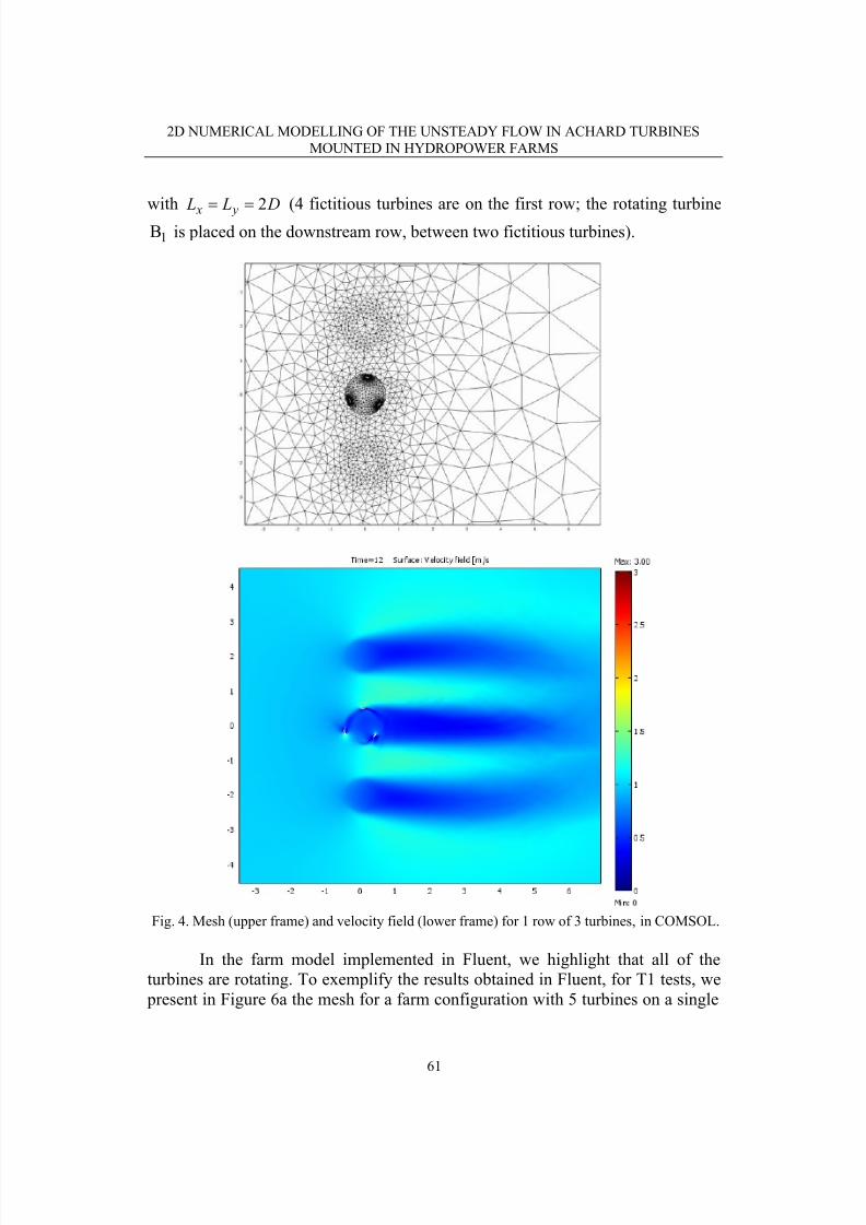
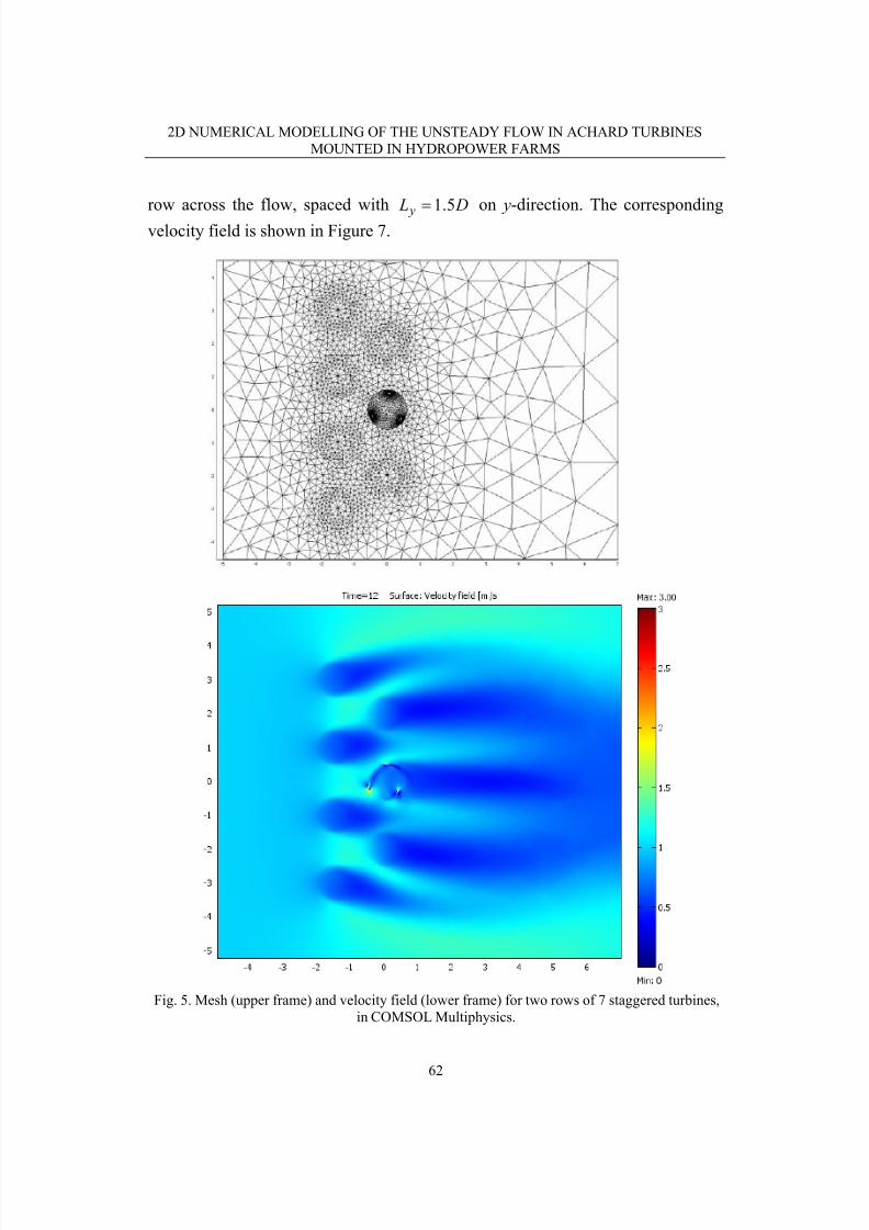
To ensure the free flow conditions around the farm, for all tested

configurations, the computational domain extension was the same, namely: 12

turbine diameters long (from 5−=x m to 7=x m along the flow direction), and

56 turbine diameters wide (from 28−=y m to 28=y m across the flow). The true

(main) rotating turbine was placed with its axis in the point of coordinates

, while the fictitious turbines were placed around it, in accordance to

the studied configuration.

( 0,0 == yx )

3. Numerical results

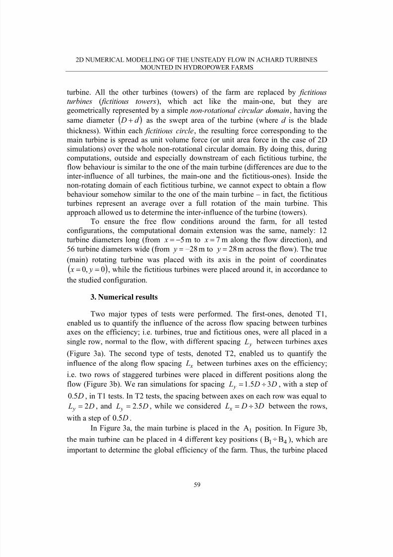
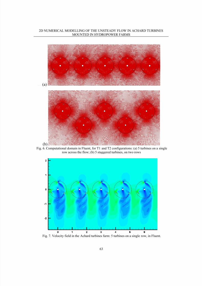
Two major types of tests were performed. The first-ones, denoted T1,

enabled us to quantify the influence of the across flow spacing between turbines

axes on the efficiency; i.e. turbines, true and fictitious ones, were all placed in a

single row, normal to the flow, with different spacing between turbines axes

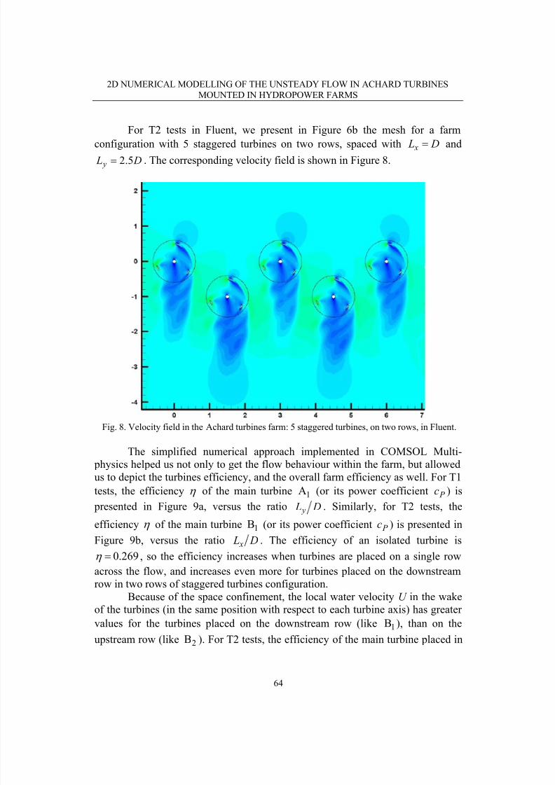
(Figure 3a). The second type of tests, denoted T2, enabled us to quantify the

influence of the along flow spacing between turbines axes on the efficiency;

i.e. two rows of staggered turbines were placed in different positions along the

flow (Figure 3b). We ran simulations for spacing

yL

xL

DDLy 35.1 ÷= , with a step of

, in T1 tests. In T2 tests, the spacing between axes on each row was equal to

, and , while we considered

D5.0

DLy 2= DLy 5.2= DDLx 3÷= between the rows,

with a step of .D5.0

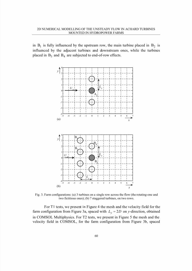
In Figure 3a, the main turbine is placed in the position. In Figure 3b,

the main turbine can be placed in 4 different key positions ( ÷ ), which are

important to determine the global efficiency of the farm. Thus, the turbine placed

1A

1B 4B

59





in1

B is fully influenced by the upstream row, the main turbine placed in2

B is

influenced by the adjacent turbines and downstream ones, while the tu es

and are subjected to end-of-row effects.

rbin

placed in 3B 4B

-5 -4 -3 -2 -1 0 1 2 3 4 5 6 7-4

-3

-2

-1

0

1

2

3

4

x

y

(a)

U ∞

Ly

A1

-5 -4 -3 -2 -1 0 1 2 3 4 5 6 7-4

-3

-2

-1

0

1

2

3

4

B1

B2

B3

B4

Lx

LyU

∞

y

(b) x

gurations: (a) 3 turbines on a single row across the flow (theFig. 3. rm confi rotating-one and

esh and

Fatwo fictitious ones); (b) 7 staggered turbines, on two rows.

For T1 tests, we present in Figure 4 the m the velocity field for the

farm configuration from Figure 3a, spaced with DLy 2= on y-direction, obtained

in COMSOL Multiphysics. For T2 tests, we present in Figure 5 the mesh and the

velocity field in COMSOL, for the farm configuration from Figure 3b, spaced

60





with (4 fictitious turbines are on the first row; the rotating turbine

is placed on the downstream row, between two fictitious turbines).

DLLyx

2==

1B

Fig. 4. Mesh (upper frame) and velocity field (lower frame) for 1 row of 3 turbines, in COMSOL.

In the farm model implemented in Fluent, we highlight that all of the

turbines are rotating. To exemplify the results obtained in Fluent, for T1 tests, we

present in Figure 6a the mesh for a farm configuration with 5 turbines on a single

61





row across the flow, spaced with DLy

5.1= on y-direction. The corresponding

velocity field is shown in Figure 7.

Fig. 5. Mesh (upper frame) and velocity field (lower frame) for two rows of 7 staggered turbines,

in COMSOL Multiphysics.

62





(a)

(b)Fig. 6. Computational domain in Fluent, for T1 and T2 configurations: (a) 5 turbines on a single

row across the flow; (b) 5 staggered turbines, on two rows

Fig. 7. Velocity field in the Achard turbines farm: 5 turbines on a single row, in Fluent.

63





For T2 tests in Fluent, we present in Figure 6b the mesh for a farm

configuration with 5 staggered turbines on two rows, spaced with and

. The corresponding velocity field is shown in Figure 8.

DLx =

DLy 5.2=

Fig. 8. Velocity field in the Achard turbines farm: 5 staggered turbines, on two rows, in Fluent.

The simplified numerical approach implemented in COMSOL Multi-

physics helped us not only to get the flow behaviour within the farm, but allowed

us to depict the turbines efficiency, and the overall farm efficiency as well. For T1

tests, the efficiency η of the main turbine (or its power coefficient1A P c ) is

presented in Figure 9a, versus the ratio DLy . Similarly, for T2 tests, the

efficiency η of the main turbine (or its power coefficient1B P c ) is presented in

Figure 9b, versus the ratio DLx . The efficiency of an isolated turbine is

269.0=η , so the efficiency increases when turbines are placed on a single row

across the flow, and increases even more for turbines placed on the downstream

row in two rows of staggered turbines configuration.

Because of the space confinement, the local water velocity U in the wake

of the turbines (in the same position with respect to each turbine axis) has greater

values for the turbines placed on the downstream row (like ), than on the

upstream row (like ). For T2 tests, the efficiency of the main turbine placed in

1B

2B

64





the 4 key positions, for the 2=DLx

ratio, has the following values: 443.0=η

for ;1B 263.0=η for ;2B 268.0=η for and3B 303.0=η for , obviously

the most advantaged position being . The resulting global farm efficiency is

4B

1B

317.0≅η . Extrapolating, the global farm efficiency increases when increasing the

number of turbines, e.g. 341.0≅η for 21 staggered turbines on 2 rows.

1. 5 1 .6 1 .7 1. 8 1 .9 2 2 .1 2. 2 2 .3 2 .4 2 . 5 2 .6 2 .7 2 .8 2. 9 30.28

0.285

0.29

0.295

0.3

0.305

0.31

0.315

(a) Ly/D

η or cP

2 2.1 2.2 2.3 2.4 2.5 2.6 2.7 2.8 2.9 30.41

0.415

0.42

0.425

0.43

0.435

0.44

0.445

0.45

(b) Lx/D

η or cP

Fig. 9. Efficiency η or power coefficient of: (a) turbine ; (b) turbine , versus the

spacing between turbines in number of turbine diameters.P c 1A 1B

The evolution of the local velocity in the turbine wake at the position( ), meaning at one diameter downstream of the axis, during the 12

seconds of simulation time (representing 6 full rotations of the turbines) is plotted

in Figure 10 for ’s turbine wake. From the local velocity temporal evolution in

the turbine wake plotted in Figure 10, obtained in COMSOL Multiphysics, one

can see that the flow is stabilized after the first 4 full rotations of the turbines –

that is, after 8 seconds from the start of the simulation.

0,1 == yx

1B

4. Conclusions

The study pointed on the Achard turbine – a new concept of vertical axis

cross-flow current turbine. The 2D numerical modelling of the unsteady flowinside a hydropower farm, equipped with several Achard turbines placed on a

single row across the flow, or in staggered configurations on two parallel rows,

has been performed using both COMSOL Multiphysics, and Fluent.

The horizontal distances between axes of the cross-flow turbines (or

turbine towers) mounted in hydropower farms play a major role in turbines

efficiency. The efficiency of the turbines increases as the turbines get closer to

each other, especially on the downstream row.

65





Fig. 10. Local velocity U in ’s wake versus time1B

The method implemented in COMCOL Multiphysics has proven to save a

lot of computational time, with respect to the total computational time requested

in Fluent when all the turbines are rotating. In COMSOL Multiphysics, a

computation with 7 rotating turbines would have taken several days, while, by

using the simplified approach, all computations took less than 10 hours.

R E F E R E N C E S

[1] J.-L. Achard, T. Maître, Turbomachine hydraulique. Brevet déposé, Code FR 04 50209,Titulaire: Institut National Polytechnique de Grenoble, France, 2004.

[2] A.-M. Georgescu, Sanda-Carmen Georgescu, S. I. Bernad et al., Interinfluence of the verticalaxis, stabilised, Achard type hydraulic turbines (THARVEST). CEEX Project no 192/2006,

AMCSIT Politehnica Bucharest, http://www.tharvest.ro, 2006-2008.[3] Sanda-Carmen Georgescu, A.-M. Georgescu, S. I. Bernad , Innovative simplified 2D numerical

modelling of the inter-influence of vertical axis cross-flow turbines mounted in hydropower farms, in Scientific Bulletin “Politehnica” University of Timisoara, Transactions on

Mechanics, vol. 53(67), fascicola 3, 2008, pp 57-62.[4] A.-M. Georgescu, Sanda-Carmen Georgescu, S. I. Bernad , L. V. Haşegan, Staggered

arrangement of three bladed, vertical axis, cross-flow turbine towers in farms, in Sci. Bull.“Politehnica” Univ. Timisoara, Trans. Mechanics, vol. 53(67), fascicola 3, 2008, pp 63-68.

[5] S. I. Bernad , T. Bărbat, A.-M. Georgescu, Sanda-Carmen Georgescu, R. Susan-Resiga,Unsteady flow simulation in the Achard turbines mounted in hydropower farms, in Sci.Bull. “Politehnica” Univ. Timisoara, Trans. Mech., vol. 53(67), fascicola 3, 2008, pp 69-74.

[6] A.-M. Georgescu, Sanda-Carmen Georgescu, M. Degeratu, S. Bernad , C. I. Cosoiu, Numericalmodelling comparison between airflow and water flow within the Achard-type turbine, inSci. Bull. “Politehnica” Univ. Timisoara, Trans. Mech., vol. 52(66), f. 6, 2007, pp 289-298.

66

http://hidraulica.utcb.ro/tharvest/en/index.html

http://hidraulica.utcb.ro/tharvest/en/index.html

Date post:	08-Apr-2018
Category:	Documents
Upload:	prabal-negi
View:	222 times
Download:	0 times

2D numerical modelling of the unsteady flow in the achard turbines mounted in hydropower farms

Documents